Article

Effects of Coastal Urbanization on Habitat Quality: A Case Study in Guangdong-Hong Kong-Macao Greater Bay Area

1
State Key Laboratory of Resources and Environmental Information System, Institute of Geographic Sciences and Natural Resources Research, Chinese Academy of Sciences, Beijing 100101, China
2
College of Resources and Environment, University of Chinese Academy of Sciences, Beijing 100101, China
3
School of Earth Science and Technology, Zhengzhou University, Zhengzhou 450001, China
4
School of Geography and Ocean Sciences, Nanjing University, Nanjing 210023, China
*
Author to whom correspondence should be addressed.
Land 2023, 12(1), 34; https://doi.org/10.3390/land12010034
Submission received: 2 December 2022 / Revised: 15 December 2022 / Accepted: 18 December 2022 / Published: 23 December 2022
(This article belongs to the Special Issue Ecosystem-Based Regional Planning)

Abstract

:
Coastal areas are usually considered as pioneering areas for economic development and reform due to their unique geographical locations and ecological conditions. Correspondingly, rapid urbanization in coastal urban agglomerations has resulted in population concentration and land use/cover change (LUCC), leading to the decline of habitat quality and biodiversity. However, few studies have quantitatively explored the impacts of urban agglomeration expansion in coastal zones on habitat quality. Taking the Guangdong-Hong Kong-Macao-Great Bay Area (GBA) as a case study, we applied the Integrated Valuation of Ecosystem Services and Trade-offs (InVEST) model to assess the habitat quality based on land use data obtained from remote sensing images from 1980 to 2020 and developed a geographically weighted regression model to quantitatively analyze the response of habitat quality to urbanization. The results showed that (1) LUCC in the GBA was dramatic from 1980 to 2020, dominated by the shift from various land use types to construction land, which led to increased fragmentation; (2) the overall habitat quality showed a decreasing trend, characterized by low values in the central part and high values in the surrounding area; (3) population and construction land such urbanization elements had a more significantly negative effect on habitat quality changes, while the relationships among slope, road distance, and habitat quality changes were complex. Based on above analysis, this paper suggests that future land management in the GBA should develop in the direction of intensification, refinement, and regional integration.

1. Introduction

Coastal zones are interaction areas between terrestrial and marine ecosystems [1]. Their unique geographical locations and abundant natural resources make them important biological habitats, as well as key zones for urbanization and economic development [2]. With the continuous advancement of urbanization, land use changes caused by population concentration and industrial and infrastructure construction have led to habitat fragmentation and loss, thereby affecting biodiversity [3,4,5,6]. Furthermore, this trend has been getting worse over the past years [7]. Previous studies have suggested that coastal cities are expanding exponentially [8] and the loss of ecosystem services is particularly prominent in coastal zones [9]. Therefore, it is necessary to understand the state and variation process of habitat quality in coastal agglomerations and then to analyze the mechanism of habitat quality degradation due to urban expansion [10].
Land use and land cover change (LUCC) is the main threat to biodiversity loss, which is closely related to habitat quality decline [3,4,11]. Habitat quality is a core indicator of eco-environmental level [12]. Relevant studies are mainly based on LUCC, investigating the spatial and temporal evolution of habitat quality [13], taking scene simulations using urban expansion models (e.g., the Conversion of Land Use and its Effects at Small Region Extent model and the Cellular Automata model) [14,15], constructing regional ecological security patterns [16], and predicting the future direction of ecological patterns [17]. Researchers have found that the unpromising LUCC trend (i.e., the rapid increase of construction land and significant decrease of wetlands) has a close relationship with socio-economic development [1,18]. What deserves to be noticed is that this pattern is the result of rapid urban expansion [1]. In addition, urbanization also results in the decrease of landscape connectivity and the increase of fragmentation [19,20]. Studies on habitat landscape changes in cities are critical for biodiversity conservation [19,21]. Landscape analysis focuses on the type, shape, distribution, and arrangement of ecosystem components under different land cover conditions, which can reveal the urbanization effect on habitats inspatial dimension [14,18,22]. Different from other methods for monitoring variations in landscape patterns, i.e., land use models and remote sensing, the landscape index can provide precise information about landscape configuration and patterns [14,23]. It is a common method for quantitatively describing landscape fragmentation, diversity, and structure. However, while most researchers have explored the impacts of LUCC on habitat quality, study on spatial heterogeneity at a landscape level is scarce [22]; This issue needs to be addressed [22,24,25].
Habitat quality refers to the capacity of an ecosystem to provide the conditions for species to survive and multiply, reflecting the level of ecosystem services as an important aspect of biodiversity [26,27,28]. Habitat quality assessments have become an important component in assessments of ecosystem services [7]. They can help us understand the carrying capacity of regional ecosystems and the welfare gained by humans, making it possible to construct a sustainable management pattern [5,29]. Calderon and An analyzed the effects of pool, riffle, and run ecosystems on fish [30]; Cuffney et al. assessed the responses of benthic macroinvertebrates to urbanization and LUCC by field reconnaissance and according to various indicators [31]. Previous studies on biodiversity have mainly been conducted in the form of field surveys. Due to its high cost in terms of time and labor, this method is not suitable for large-scale studies [32]. In recent years, with progress in computer technology, GIS, and remote sensing technology, more attention is being paid to the dynamic monitoring of habitat quality on a large scale [12,25]. In this regard, there are two common methods: the first adopts an index system, e.g., the analytical hierarchy process, fuzzy comprehensive evaluation, and artificial neural networks [33,34,35]; the second includes ecosystem models, such as the Habitat Suitability Index model, Social Values for Ecosystem Services model, Integrated Valuation of Ecosystem Services and Trade-offs (InVEST) model [36,37,38], etc. Among them, the InVEST model generates habitat quality maps based on LUCC and the distribution of threat factors [39,40]. It is widely used to quantify habitat quality in different regions and on different scales due to its ease of use and flexible output [41,42].
Rapid coastal urbanization in recent years has profoundly affected land use patterns, resulting in the reduction of ecological land; this trend will continue [7]. Therefore, the influence of human activities, especially urbanization, on coastal ecosystems has become a hot spot in recent years. Numerous studies have explored the impact of coastal urbanization on regional ecosystems from the perspectives of ecological patterns, land use, and landscapes. Mayer-Pinto et al. investigated the structure and function of microbial communities in artificial and natural coastal environments [43]. They focused on how the differences between the two ecosystems were reflected in biodiversity changes. Dupras et al. studied the variation of ecosystem services on the Mediterranean coast based on LUCC [44]. Aguilera et al. investigated the effects of urbanization on coastal ecosystem spatial connectivity from a landscape pattern perspective [45]. More and more studies have shown that urbanization has led to coastal ecosystem degradation. Therefore, land use optimization seems to be necessary in urban construction. Common methods with which to analyze the influence of urbanization on habitat quality include correlation analysis [46], regression model [45], and index appraisal [1]. These approaches are appropriate for solving questions about the impact of a single factor (e.g., land use conversion) on habitat quality but are not suitable for analyses of the extent and direction of natural and social factors in the process of urbanization. Some studies have noted that habitat loss caused by LUCC is the result of interactions between natural ecosystems and humans. Such influences of LUCC are usually spatially autocorrelated because of their similar geographical environments [47]. The geographically weighted regression (GWR) model introduces the location attributes into regression analysis; it is a robust method for solving problems about spatial heterogeneity [48,49]. Currently, the GWR model is being used in various spatial correlation studies. Su et al. analyzed the spatial changes between agriculture landscape and urbanization; those authors noted that the GWR model has better explanatory accuracy and yields richer information [50]. Shearmur et al. also used it to explore the spatial and temporal differences behind the reasons for employment growth in Canada, showing that the model has strong explanatory power for socioeconomic problems [51].
The Guangdong-Hong Kong-Macao Greater Bay Area (GBA), which borders on the South China Sea, is one of the most economically open and active regions in China. Over the past four decades, it has experienced rapid urbanization and dramatic LUCC, which has placed increasing pressure on regional ecological areas and biodiversity [52,53,54]. To this end, taking GBA as a case study, the aim of this study is to fill in the gap in habitat quality assessments during the period of rapid coastal urbanization. The research objectives of this study are: (1) to analyze the rate and direction of land use changes in GBA; (2) to investigate the landscape pattern features and variation tendency; (3) to explore the spatial-temporal evolution characteristics of habitat quality from 1980 to 2020; and (4) to quantitatively reveal the impact of coastal urbanization on habitat quality based on the dimensions of nature and society.

2. Materials and Methods
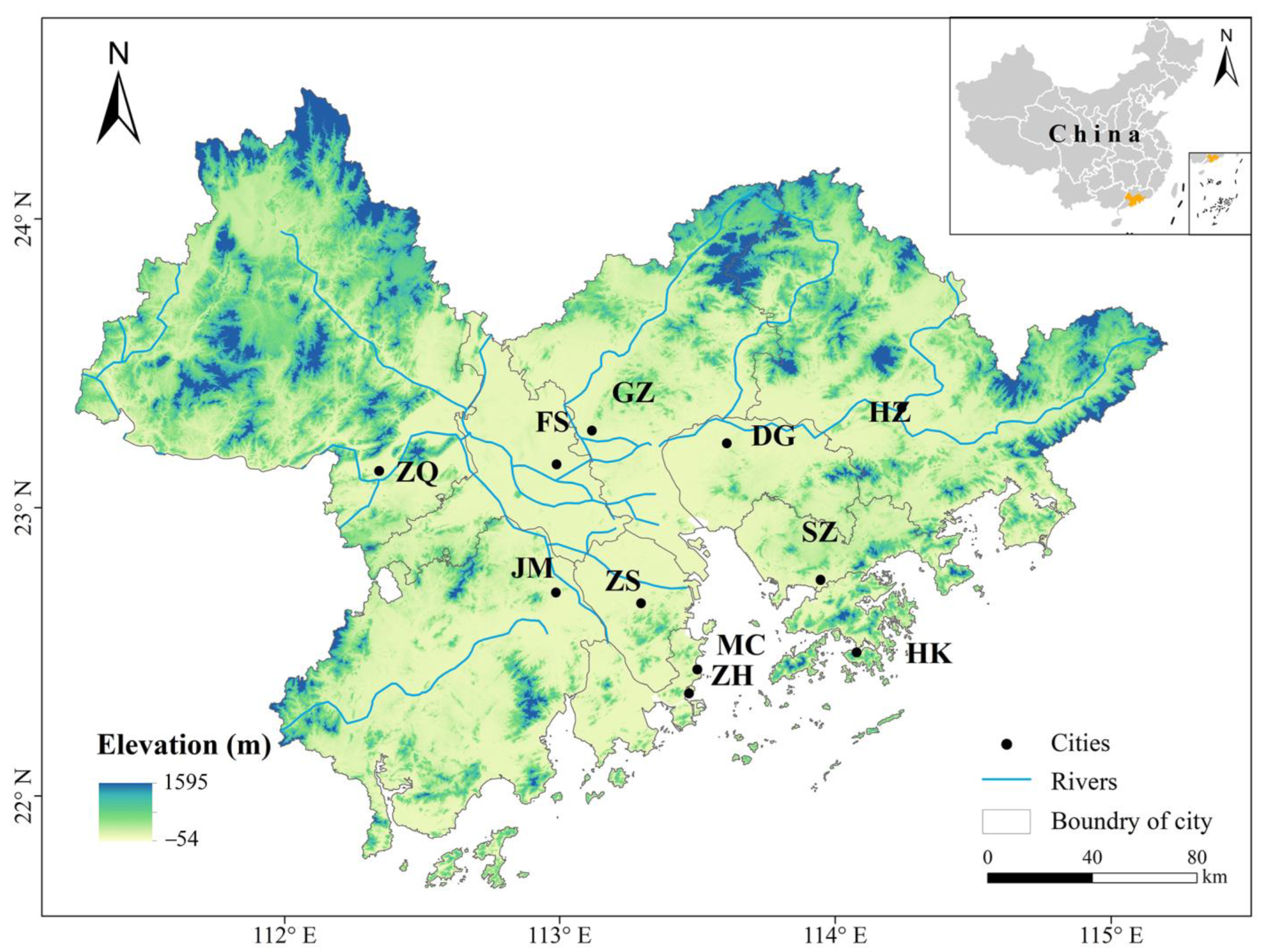
2.1. Study Area

The GBA (21°17′ N–23°55′ N, 111°59′ E–115°25′ E) is a cluster of nine cities in Guangdong Province, namely, Guangzhou, Jiangmen, Zhaoqing, Zhuhai, Shenzhen, Huizhou, Dongguan, Foshan, and Huizhou, as well as the two special administrative regions of Hong Kong and Macao. It is located in southern China, at the intersection of the Pearl River and the South China Sea, with a long coastline and vast maritime area (Figure 1). The GBA covers approximately 56,000 km2. The east, north, and west sides are surrounded by hills, with plains in the center and southeast. GBA is the fourth largest bay area in the world after the New York Bay Area and the San Francisco Bay Area in USA and the Tokyo Bay Area in Japan. As such, it is an important carrier for the country to construct a world-class city cluster and participate in global enterprise. In 2020, the total population of the GBA exceeded 86 million, the regional gross domestic product (GDP) reached 166.88 billion dollars, and the urbanization rate reached over 80% (Guangdong Provincial Bureau Statistics and Survey office of the National Bureau of Statistics in Guangdong, 2021). The “Outline Development Plan for the GBA”, released in 2019, pointed out the need to develop an international first-class bay area for living, working, and travelling, which underlined the urgency of the eco-environmental protection.

2.2. Data Sources and Preparation

The datasets in this study mainly included the following three aspects:
  • Land use data: Land use data of study area for 1980, 1990, 2000, 2010, and 2020 were obtained from the Land use and Land Cover of China (CNLUCC) data provided by the Resource Environment Science and Data Center of the Chinese Academy of Sciences (https://www.resdc.cn/, accessed on 1 July 2022), with a spatial resolution of 30 m. CNLUCC data based on Landsat TM series remote sensing images were processed using the supervised classification method, with an accuracy of more than 90% [55]. According to the present research needs and the Chinese land resource classification system, we reclassified the original land cover types into six categories: cultivated land, forestland, grassland, water bodies, construction land, and unused land. The spatial distributions of land use types in the GBA from 1980 to 2020 are displayed in Figure 2.
  • Socioeconomic data: Raster datasets of population density in 1990, 2000, and 2010 were obtained from the same source as above, with a spatial resolution of 1 km (Figure 3a–c). For the missing data, we calculated the weights of each district and county, referred to statistical yearbooks, and completed them according to adjacent years. The vector data of administrative boundaries and roads came from the National Geomatics Center of China (https://nfgis.nsdi.gov.cn/, accessed on 1 July 2022). Considering that the changes of roads were not obvious during a certain period, we only chose Road I and II in two periods (Figure 3d), corresponding to the periods of 1980–2000 and 2000–2020, respectively.
  • DEM data: SRTM elevation data, with a spatial resolution of 30 m, were obtained from the official website (https://earthexplorer.usgs.gov/, accessed on 1 July 2022). The slope data of study area were generated from DEM, as shown in Figure 3e.

2.3. Methods

2.3.1. Analysis of Land Use Change

Land use transfer matrices can quantitatively describe the land use type and status in a certain period. We used the overlay analysis tool in ArcGIS to calculate the land use transfer matrix for different periods and analyzed the intensity of land use changes based on the land use dynamic degree.
A single land use dynamic degree represents an increase or decrease of a specific land use type area during the study period [56]. The calculation formula is as follows:
K = LU b LU a LU a
where LU a and LU b denote an area of the same land use type at the beginning and end of the study period, respectively.
Comprehensive land use dynamic degree (LC) quantitatively describes the land use change rate in a particular period, reflecting comprehensive changes in land use area [32,57]. The formula is as follows:
LC = i = 1 n LU ij 2 i = 1 n LU i × 1 T × 100 %
where LU i represents the land use area at the initial time and LU ij represents the land use area converted from type i to type j within period T .

2.3.2. Landscape Index

It is essential to consider whether the indices are independent when selecting them. In order to describe the fragmentation, aggregation, dominance, and diversity of landscapes, we selected indices at the class and landscape levels, as shown in Table 1 [58], which were calculated in the Fragstats 4.2 software.

2.3.3. Habitat Quality Assessment Model

The InVEST habitat quality model assesses habitat quality and the threat degree to biodiversity based on LUCC, which is reflected in the habitat quality index, ranging from 0 to 1; the larger the value, the better the habitat quality. The formula is as follows:
Q xj = H j [ 1 ( D xj z D xj z + k z ) ]
where Q xj is the habitat quality of grid x in land use type j ; H j is the habitat adaptability of land use type j ; z and k are the normalization constant and half-saturation constant, respectively; and D xj is the habitat degradation degree, defined as follows:
D xj = r = 1 R y = 1 Y r ( ω r r = 1 R ω r ) r y i rxy β x S jr
where R and Y r indicate the number of threat factors and grids, respectively; ω r is the weight of threat factor r ; r y is the threat value of grid y ; i rxy indicates the impact of threat value r y in grid y on habitat grid x ; β x is the anti-interference level of the habitat; and S jr is the relative sensitivity of habitat type j to threat factor r .
There are two attenuation methods for i rxy , represented by the following equations:
Linear   attenuation :   i rxy = 1 ( d xy d r   max )
Exponential   decay :   i rxy = exp [ ( 2.99 d r   max ) d xy ]
where d xy is the distance between habitat grid x and threat grid y and d r   max is the maximum impact distance of threat factor r .
The input parameters of the InVEST model include land use maps for each period, threat factor data (including maximum impact distance, weight, and degradation type), threat factor maps, sensitivity of land use types to each threat, and the level of legal protection from disturbance in each grid. In this study, we considered all grids in the study area to be equally protected and mainly considered the effects of other parameters.
With this model, it is first necessary to distinguish the habitats. As reflections of human activity, construction land and cultivated land can both lead to habitat fragmentation, threatening the natural ecosystem to a certain extent. Therefore, we defined cultivated land, construction land, and unused land with low vegetation coverage such as sand, bare ground, and bare rocky land as threat sources, and forestland, grassland, and water bodies as habitats.
The parameters to be adjusted according to the specific conditions in the study area include the maximum impact distance (i.e., the weights) of threat factors, the suitability scores of different land use types, and the sensitivity to threat sources, which were determined based on the model guidebook and research results from other scholars [16,39,59,60]. The specific parameters are shown in the Table 2 and Table 3.

2.3.4. Quantitative Analysis of the Impact of Urbanization

1.
Fundamental principle
Regression analysis is a common method to explore relationships among variables. As a global regression, ordinary least squares (OLS) is based on the minimum estimated residual sum of squares to determine the regression model. It can be stated as:
y = β 0 + i = 1 k β i x i + ε
where y is the explanatory variable; β 0 is the intercept; β i is the regression parameter coefficient of independent variable x i ; ε is the random error term fitted to the normal distribution; and k is the number of independent variables.
Due to the different natural geographic conditions, regulatory policies, and effects across the study area, the impacts of urbanization on habitat quality are complex and changeable. In other words, the drivers of urbanization are spatially heterogeneous. The GWR model introduces the location attributes as distances based on weights into the regression equation, which can describe the spatial non-stationary nature of urbanization factors more precisely and make the results more reliable. Therefore, with each regression point as a center, this study established local regression equations for GWR analysis within a certain radius. It can be expressed as:
y i = β 0 ( u i , v i ) + j = 1 k β j ( u i , v i ) x ij + ε i
where ( u i , v i ) is the geographic coordination for location i ; β j ( u i , v i ) represents the regression coefficient for independent variable x j at location i ; β 0 ( u i , v i ) is the intercept; and ε i is the random error term where ε i N ( 0 , σ 2 ) .
The regression coefficient at position ( u i , v i ) is given by β ^ ( u i , v i ) :
β ^ ( u i , v i ) = ( X T W ( u i , v i ) X ) 1 X T W ( u i , v i ) Y
where W ( u i , v i ) is the spatial weight matrix.
The calculation of weights depends on the distance decay function. Gaussian function is one of the commonly used methods, which can be stated as:
ω ij = exp ( d ij b ) 2
where d ij is the distance between sample points i and j ; and b is the bandwidth.
Bandwidth is the distance band for each local regression equation. It directly affects the fitting accuracy of the model and is perhaps the most important parameter to consider for GWR [61]. This study adopted the AICc method to determine the optimal bandwidth with the minimum AIC value.
2.
Model construction
Natural elements and human activities are key factors contributing to habitat quality differentiation [53]. Firstly, terrain is generally considered to affect the density, scale, and spatial distribution of urban land [62]. Since the terrain of the study area showed obvious ring-shaped features, we considered slope as a geographical determinant of urban expansion when analyzing the direct influence of natural factors on habitat quality. Secondly, socioeconomic indicators reflect the intensity of human activities, which indirectly affect habitat quality. Among them, land urbanization, population urbanization, and transportation are the driving force, core, and carrier of urbanization, respectively [63]. Therefore, we selected the construction land area, population, and road distances as socioeconomic factors. In other words, taking the changing values of habitat quality as dependent variables, the slope, changes in construction land area, population, and road distances in different periods were chosen as explanatory variables to establish the regression model.
In order to unify the resolution, we used ArcGIS to create fishing grids with a spatial resolution of 1 km as basic units for the statistics of urban drivers and habitat quality changes in the GBA. “Near Analysis” and “Zonal Statistics” were used to calculate the average slope in each grid, changes of construction land area and population in different periods, the nearest distance from the center of a grid to an arterial road, as well as the changes of average habitat quality value in each grid. Finally, this raster layer, with a resolution of 1 km, was used as the input of the regression model. Due to the lack of data in Hong Kong and Macao, this part only considered the nine cities in the Pearl River Delta. Meanwhile, in order to reduce the influence of errors in the supplementary data, we compared the OLS and GWR results for the 1980–2000 and 2000–2020 periods to choose the optimal model.
We checked whether there were any residual explanatory variables according to the OLS output report tables generated by ArcGIS. The results showed that the VIF value of each variable was less than 10 and passed the significance test; therefore, all parameters could be used in the GWR model. In this case, we used the geographically weighted regression tools in ArcGIS and chose the AICc bandwidth method. The fitting results are shown in Table 4 and Figure 4.
It can be considered that the GWR model is a significant improvement on the OLS model when the difference of AICc values is greater than 3. The above table shows that GWR model has lower Sigma and AIC values and better goodness-of-fit, so the regression coefficient results of the GWR model were used for the impact analysis. The local R2 results for this model are shown in Figure 5. It can be seen that compared with the period of 1980–2000, the range of better fitting results from 2000 to 2020 is wider, especially in the northwest and southwest margins of the GBA. This is mainly because the changes in habitat quality were not significant in these regions from 1980 to 2000 (as discussed in detail in Section 3.3 and Section 3.4). However, in general, the selected variables are appropriate for constructing the GWR model.

3. Results

3.1. Land Use Change Characteristics

We calculated the land use dynamics and the transfer matrix in the four periods of 1980–1900 (I), 1990–2000 (II), 2000–2010 (III), and 2010–2020 (IV). The results are shown in Figure 4.
It can be seen that cultivated land, forestland, and construction land have always been the main land types in the GBA, accounting for about 90% of the total area (Figure 6a). As shown, the area proportion of each land type has undergone great changes over the years. Notably, the area of construction land has increased by 5531.29 km2, with the ratio of 4.73% in 1980 increasing to 14.79% in 2020; this land types is mainly distributed in the central and southeastern area. Its growth accelerated annually, reached the peak of 6.01% from 2000 to 2010, and then slowed down. Correspondingly, the cultivated land area showed on a general downward trend, but the rate was controlled in the last period. Although the area of unused land is decreasing at a relatively high speed year by year, the change is not significant in the whole study area due to the low area ratio. The water area was reduced after 2000 but increased slightly over the whole period. The areas of forestland and grassland were relatively stable. LC was on the rise from 1980 to 2010, increasing by 1.65 times (Figure 6b). This indicates that the rate of land use in the GBA increased significantly in this period and then slowed down. In addition, after 1990, the LC was greater than the overall dynamic degree during the study period (0.21%).
The area of cultivated land declined by 1186.74 km2 from 1980 to 1990; it was mainly converted into construction land, water bodies, and forestland (Table 5). From 1990 to 2000, the main trends were the transformation of cultivated land, forestland, and water bodies into construction land; this mainly occurred on the banks of the Pearl River (e.g., Foshan, Shenzhen, and Dongguan) (Figure 7). The scale of LUCC enlarged in this period. From 2000 to 2010, as the transformation of other land use types, especially cultivated land to construction land, continued and the level became more intense, the expansion rate of construction land reached a peak, displaying a tendency of expansion from the center to the periphery. Meanwhile, 576.60 km2 of water bodies were converted into cultivated land. This mainly occurred in Foshan, accounting for 73.68% of the total area transferred in this way.
The Sankey diagram below clearly reflects the main direction and scale of land use conversion over the years (Figure 8). Notably, over the past 40 years, the increase in construction land mainly came from the occupation of cultivated land, forestland, and grassland. The expansion mainly occurred in coastal cities and their main districts such as Dongguan, Shenzhen, the Yuexiu District of Guangzhou, the Chancheng District of Foshan, etc. At the same time, there were also conversions among cultivated land, water bodies, and forestland, due to adjustments of the agricultural structure and the implementation of a farming compensation policy.

3.2. Land Use Change from the Perspective of Landscape Indices

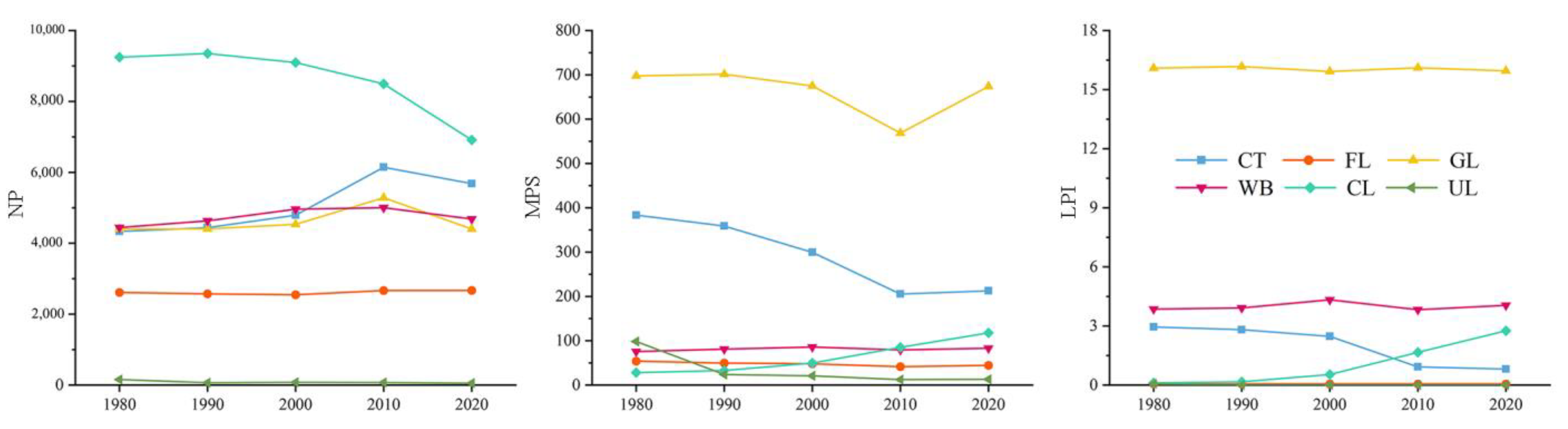
3.2.1. Class Level Analysis

Figure 9 shows the results of the landscape pattern indices at the class level. NP and MPS indicate the fragmentation of landscape classes. NP of construction land showed a downward trend, even if the values were much higher than in other classes. Additionally, MPS was relatively small but obviously increased from 2010 to 2020. This trend indicates the continuous expansion and integration of construction land, developing in spatial congregation. From 1980 to 2010, cultivated land NP increased by 41.81%, and its MPS had the greatest change, with a decrease of 46.48%. NP and MPS of water, grassland, and unused land remained steady throughout the study period, although there were some fluctuations. LPI can indirectly reflect the level of human disturbance. Although forestland LPI fluctuated very little, the changes were notably more substantial than in other classes. This indicated that forestland was the dominant landscape at the class level, and that it was not significantly influenced by human activities.

3.2.2. Landscape Level Analysis

PD reflects landscape heterogeneity in a unit area. From 1980 to 2010, PD consistently increased from 0.459 to 0.503 (Table 6). It was worth mentioning that PD decreased to 0.444 in 2020. The possible reason for this was that construction land gradually integrated and congregated from the scattered patches into large patches in that period. PAFRAC showed a peak of 1.450 in 2000, indicating the most complex patch shape at this time, before decreasing to 1.407 in 2010 and varying slightly in the other periods. SHDI is sensitive to the unbalanced distribution of landscape classes. From 1980 to 2020, SHDI increased steadily from 1.112 to 1.220, reflecting that the landscape class showed balanced development. AI decreased first then increased during the whole period. At the beginning of economic development, large-scale land resources were divided, leading to a scattered distribution. The combination and annexation of construction land patches was the main reason for the slight increase of AI after 2010.

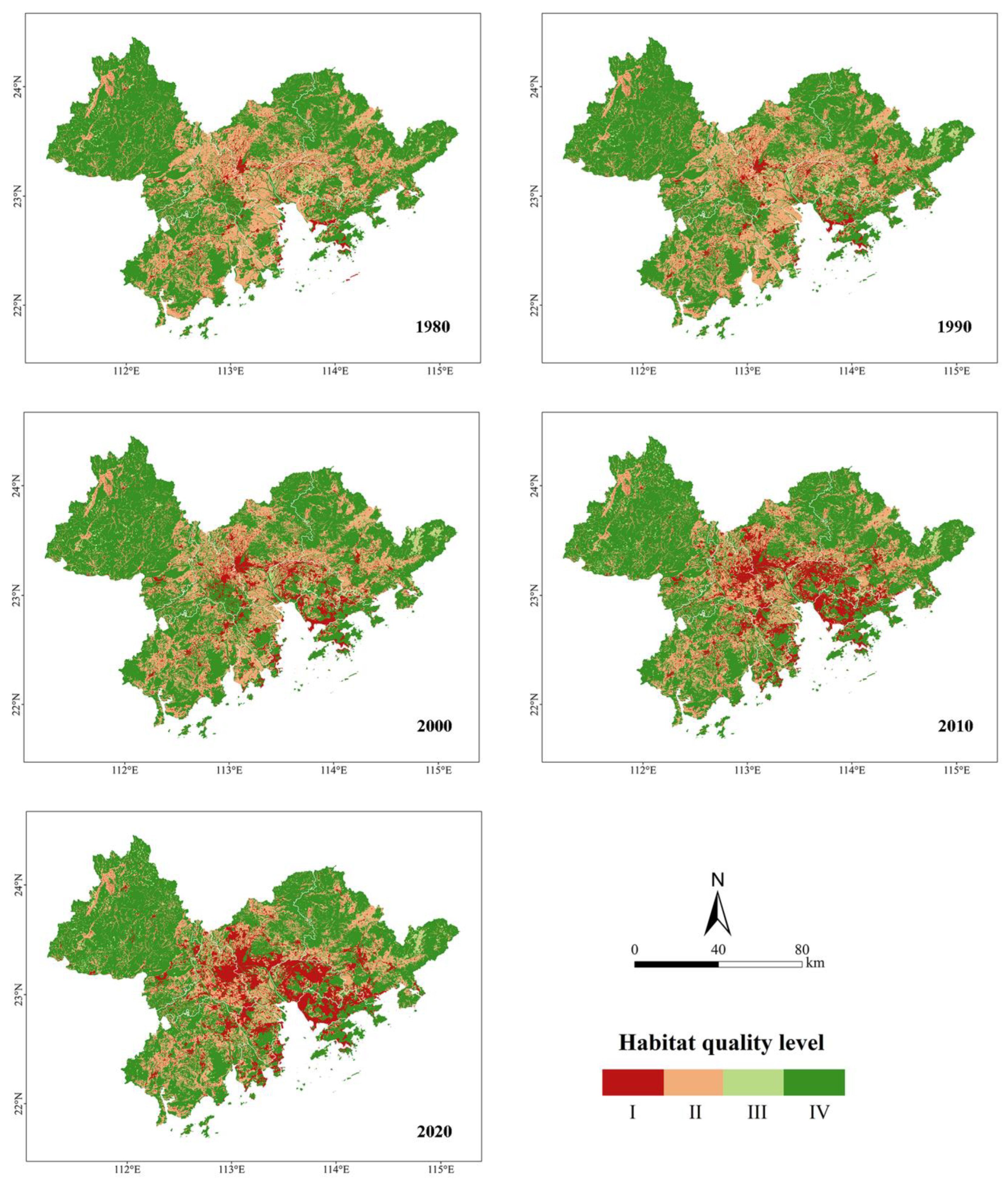
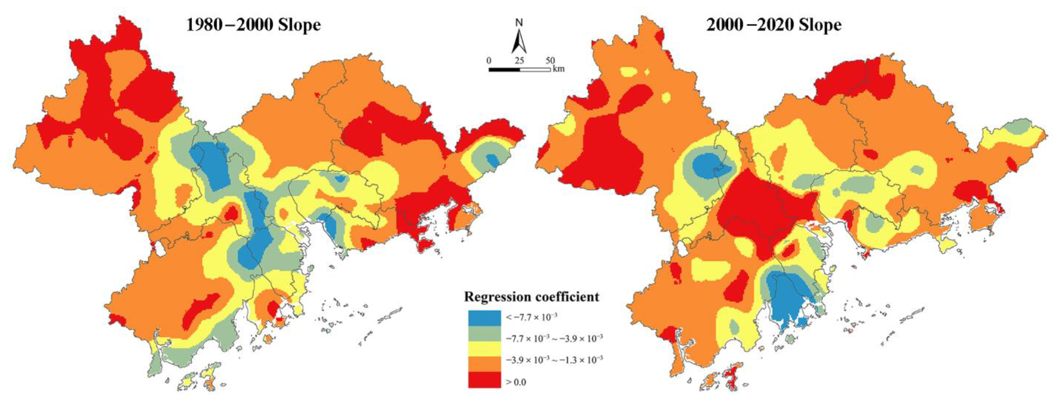
3.3. Characteristics of Habitat Quality Changes in the Context of Urbanization

In reference to the results from and reclassification methods used in previous studies, we classified habitat quality values as poor (I: 0–0.3), medium (II: 0.3–0.6), good (III: 0.6–0.8), and excellent (IV: 0.8–1) and displayed them hierarchically (Figure 10).
Spatially, it showed that the habitat quality was lower in the middle of GBA and higher in its surroundings. The level of habitat quality differed significantly within the different cities. As the leading cities, the average values of the habitat quality index in Guangdong and Shenzhen were only 0.68 and 0.60, respectively. The habitat quality of cities along the Pearl River, including Dongguan, Foshan, Zhongshan, and Zhuhai, were in the medium level (Figure 11a). Peripheral cities in GBA, including Zhaoqing, Jiangmen, and Huizhou, had better habitat quality. It is worth noting that Hong Kong still had a high level, at 0.75 or even higher, because the city has been at complete urbanization phase.
Figure 9b reveals that the average habitat quality presented a downward trend from 1980 to 2020 in the GBA. The decrease speed accelerated over the years in the first three periods, and the area proportion with poor habitat quality increased from 5.12% to 14.96% (Figure 11c). In the areas with decreased habitat quality, 5.43% of them dropped by more than 0.5, while 94.57% dropped by 0–0.5. Four cities, i.e., Dongguan, Shenzhen, Foshan and Zhongshan, experienced the most significant decline, with decreases of 40.81%, 37.21%, 26.80%, and 19.93%, respectively.

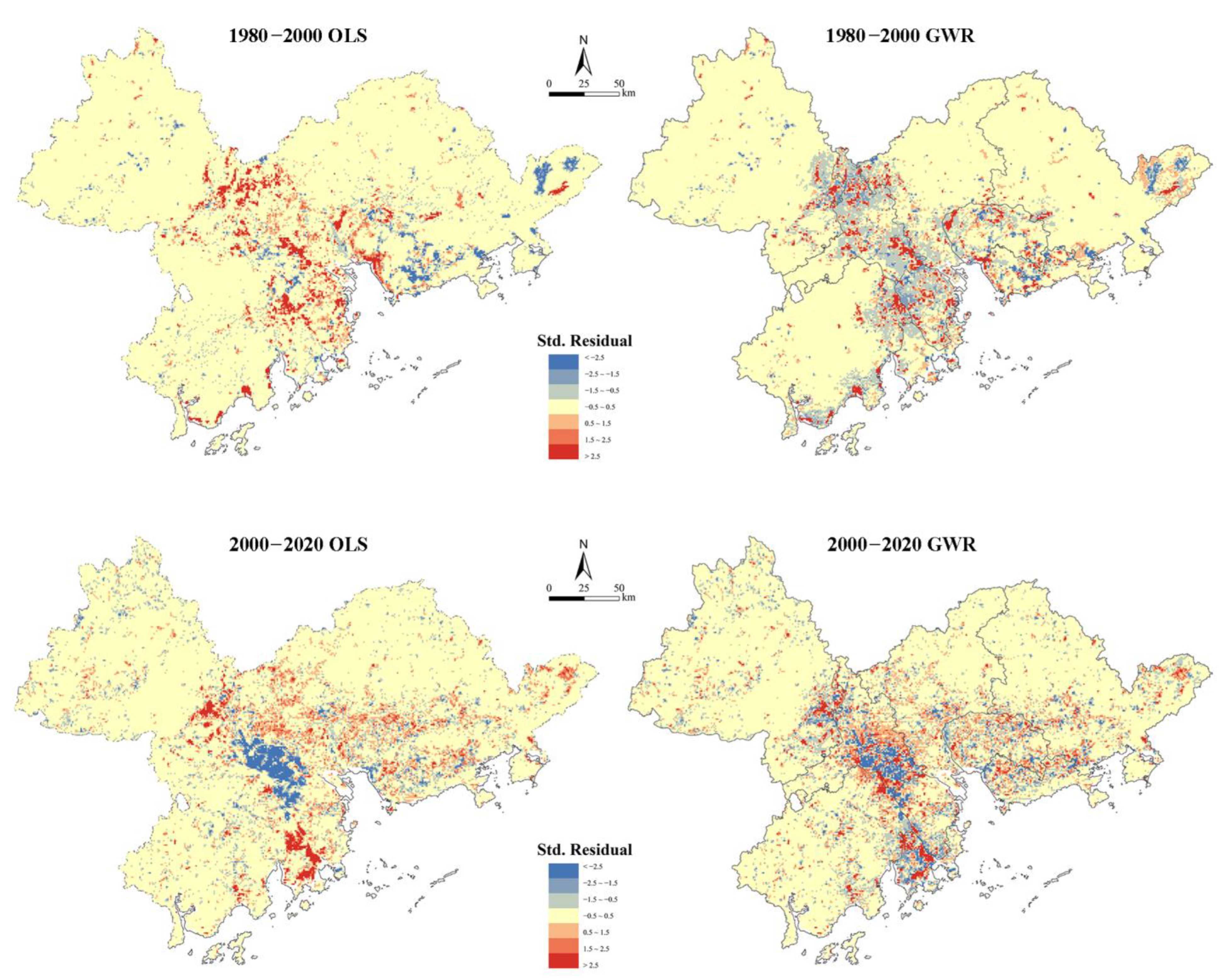
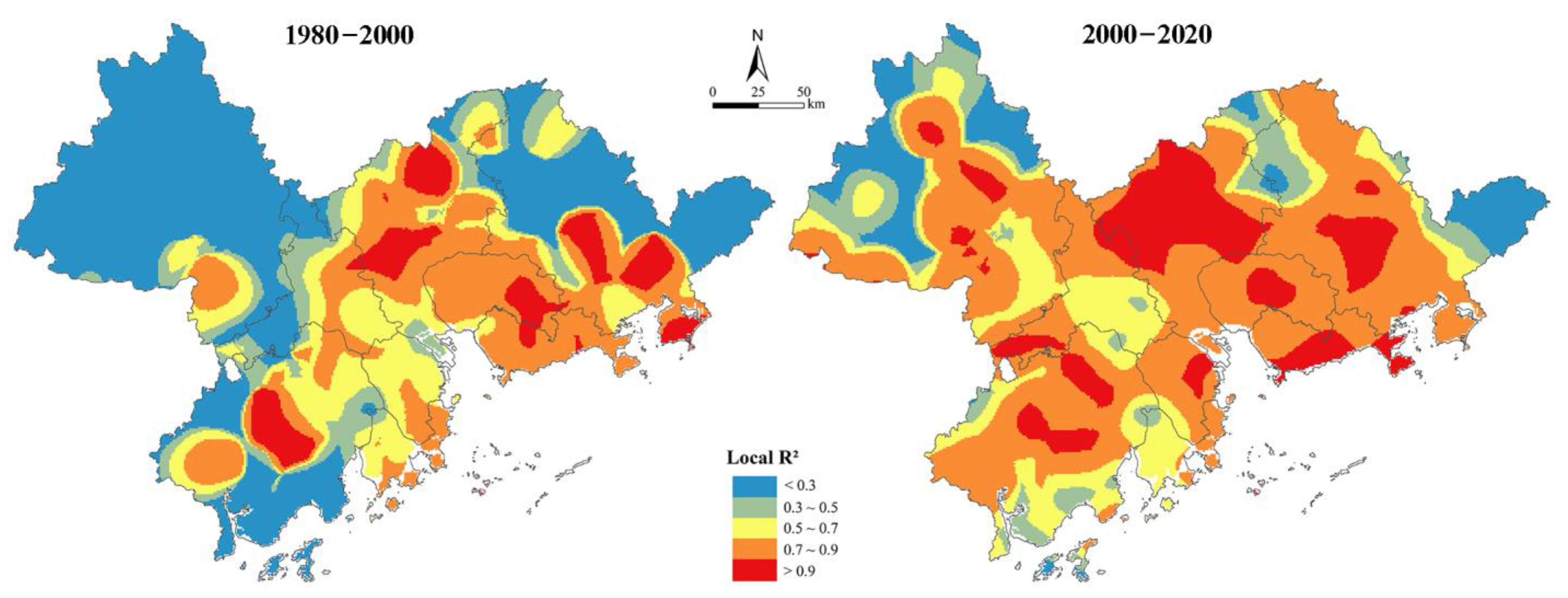
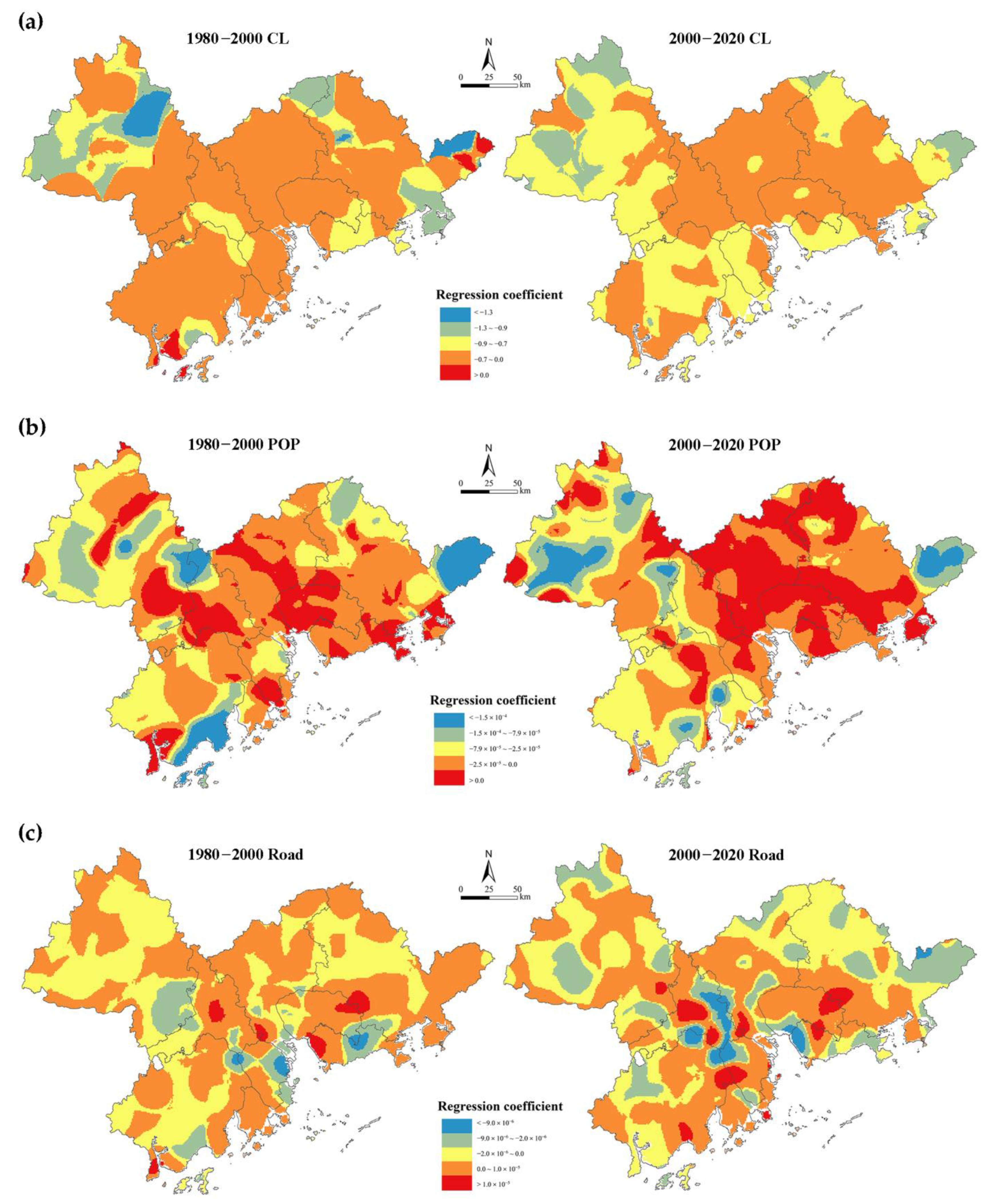
3.4. Habitat Quality Response to Urbanization Factors

3.4.1. Impact of Natural Factors

The regression coefficients between slope and habitat quality differed significantly within the two phases (Figure 12). Generally, the extreme values of coefficients were greater than the marginal zones in the central and southeastern areas with less slope than the marginal zones. Initially, the significant negative correlation was mainly distributed in the central and southern cities, including Foshan, Zhongshan, and Dongguan. After 2000, the dependence of the slope coefficient on habitat quality changed to a positive correlation, and the range of significant negative impact expanded to the surrounding areas.

3.4.2. Impact of Socioeconomic Factors

The expansion of construction land mainly came at the expense of cultivated land, which was the chief reason for habitat quality reduction. The variation of habitat quality was significantly negatively correlated with construction land, which was distributed widely (Figure 13a). Although the previous regression result exhibited greater extreme coefficient values, the negative area was extended to the entire GBA from 2000 to 2020. Notably, most areas, and in particular, Shenzhen, Guangzhou, and Zhongshan, experienced significant habitat quality degradation due to the increasing impacts of construction. Population also had a negative effect on habitat quality. (Figure 13b) The negative correlation was most prominent in the cities with relatively low population densities and extensive vegetation coverage, such as Zhaoqing, Jiangmen, and Huizhou, because the habitat quality there was more sensitive to population growth. Transportation is a critical foundation for urbanization. Road construction usually results in the degradation and fragmentation of the ecological environment. The relationships between road distance and habitat quality were varied in different places (Figure 13c). From 1980 to 2000, the negative impact was concentrated in the cities with denser road webs such as Foshan, Zhongshan, and Shenzhen. Along with the improvement of transportation infrastructure, the road network became denser and denser, and the area with negative impact expanded further. This influence was more notable in Guangzhou, which has become an important transportation city.

4. Discussion

4.1. Spatial Pattern of Habitat Quality

The terrain conditions of the GBA shape the distribution pattern of habitat quality as “higher in the middle and lower in the surroundings”. In the vast central plains, frequent human activities and large-scale land reclamations have accelerated the disturbance of habitats, resulting in a lower level of habitat quality. Relatively complete forest and grassland resources are abundant in the western and northeastern areas with more mountains and hills, which provide a good basis for biodiversity. Moreover, the scale of land use change was small within the whole city; thus, the level of habitat quality was higher in the marginal cities than that in the central cities. Additionally, over a long period of time, cities of the east coast of the Pearl River, represented by Shenzhen, Dongguan, and Huizhou, developed faster than those on the west coast [64]. More fragmented patches with low habitat quality were concentrated in the southeastern hinterland. In a word, in areas with higher development levels and economic vitality, the negative impacts of human activities on the natural environment are greater, and thus, the decline in habitat quality is more significant. The same applies within cities. The most intensive socioeconomic activities are concentrated in central urban areas, and the patches with low habitat quality tend to spread around these areas.

4.2. Drivers of Habitat Quality Change

Our results are consistent with previous research, suggesting that during rapid urbanization, excessive human activities and the increase of demand for construction land to support development accelerate the evolution of land use patterns, directly resulting in significant habitat quality degradation [40,65,66]. In terms of indirect factors, based on previous studies, we consider that geographical conditions form the foundation of urbanization, as they determine the orientation of urban development to a certain extent [53,57]. Policy guides the development of urban agglomeration [67]. Population growth and road construction are the driving forces for urban expansion. In 1980, the pattern of opening up this coastal area, marked by the foundation of the Special Economic Zone, was initiated, and the road network in China began to expand from that time. Economic development and transportation construction mutually promoted each other, providing the conditions for population flow [68]. The massive influx of immigrants and the growth of the non-agricultural population were often associated with the rapid expansion of residential and commercial land. At this time, the region was still in the initial stage of economic construction. The rate of land use change grew with the increase in land demand. With the growth of industry and commerce and the stimulating effect of the real estate craze, various activities divided and occupied large swathes of cultivated land and forestland. The expansion of construction land came at the cost of land use types with higher habitat suitability. This process has destroyed the relative integrity and connectivity of land resources and led to habitat degradation. The period of 2000–2010 saw the most rapid urban development and economic growth. Excluding Hong Kong and Macao, the gross regional product of the nine cities in the Pearl River Delta increased from 847.129 billion yuan to 380.2846 billion yuan, and the population increased from 42.8978 million to 56.2295 million. The extent and speed of land use change reached a peak during this period. On the one hand, the agglomeration effect of urban development caused construction land to expand from the main urban area to the surrounding area, showing the trend of spatial concentration. On the other hand, non-agricultural construction and agricultural structure adjustments accelerated the fragmentation of cultivated land and forest patches. Forestland reclamation and the replacement of dike ponds with highly economically beneficial construction land were common. At the same time, in order to compensate for the cultivated land that was lost during the early industrial development, large-scale land reclamation from beaches or the sea led to a significant reduction of water bodies. This was considered one of the main causes of habitat quality decline in this period. Additionally, road construction has contributed to the population concentration, leading to landscape fragmentation and the reduction of biological habitats, which have further deepened the negative impact on habitat quality [14]. After 2010, economic growth tended to be stable and urban development reached a level of maturity. With an increase of governmental supervision and ecological regulations, urban planning has become more rational. Additionally, regional ecological degradation and habitat quality decline have been effectively limited. Especially since the implementation of the Pearl River Delta Reform and Development Plan, cities have intensified their land management and construction activities. The disordered sprawl of construction land has also been controlled. For Hong Kong and Macao, conservation areas, such as urban catchments and country parks, were delimited at the beginning of planning. Thus those cities still show a relatively stable level of habitat quality for high-density cities.
Our study provides a new perspective for analyzing the relationship between the urbanization process and changes in habitat quality caused by LUCC. Compared with previous studies, this paper takes spatial heterogeneity into consideration. Combined with a dynamic analysis of regional landscapes, it reveals the spatial characteristics and underlying process of urban expansion and clearly reflects the spatial variability of such impacts [22,47]. However, there are some limitations in this study. For example, to ensure the consistency of the research scale, we set the grid size to 1 km × 1 km in the regression model but neglected the fact that some landscape indices are sensitive to resolution. Furthermore, the threat factor in the InVEST model is subjective because of the difficulty in obtaining direct observation data; thus, there is room for improvement in the applied model.
The impact of urbanization on the environment is complex and variable. It is essential to focus on LUCC in long time series and take the effects of various factors into consideration, so as to make more targeted decisions of land management. This requires further studies on how to select landscape indices and set parameter values in order to reflect evolution features more precisely in the study area.

4.3. Proposals for Optimizing Urban Land Management

Through our results, it can be seen that the rapid expansion of construction land in the GBA from 1980 to 2020 has squeezed numerous ecological spaces. The main threat to regional ecological security has come from urbanization development and increasingly intense human activities, making the ecological environment foundation more fragile. Coastal lands managed and developed in a sustainable manner can provide national and regional benefits, notably in terms of achieving the Sustainable Development Goals (SDGs) [69]. Therefore, it is essential to divide functional areas rationally, exploit land resources moderately, and harmonize the relationship among cultivated land, construction land, and ecological land; this aspect deserves more attention from long-term urban development decision makers. With these issues in mind, according to the specific development features of the corresponding cities, a few suggestions for land management in the GBA are proposed:
  • As the pilot cities of eco-environmental protection and policy reform, Guangdong and Shenzhen are required to integrate scattered land resources and improve land utilization efficiency. From an urban planning perspective, governments should divide areas by function and specify land use types (e.g., residential land, industrial and mining land, ecological protection land). Furthermore, it is urgent to establish red lines for construction land increments and strengthen the penalties for illegal construction. Meanwhile, governments should enhance cooperation with Hong Kong and Macao in ecological protection, promote the construction of public Transport-Oriented Development (TOD), and encourage green roof construction by learning from foreign experience. The ultimate goal is to achieve intensive and efficient development of mega-cities in the future.
  • In the four cities along the Pearl River, i.e., Foshan, Dongguan, Zhongshan, and Zhuhai, reclamation activities of tidal flats and sea are common. Local governments should pay attention to the protection of coastal tidal flats and promote post-cultivation management. As for inter-provincial cooperation, it should rely on neighboring cities, strive to enhance cross-administrative cooperation in land planning, and strengthen wetland protection.
  • Forestland resources are widely distributed in Zhaoqing, Jiangmen, and Huizhou, acting as ecological barrier for the GBA. These cities should develop a scientific and operational protection system for their natural resources, e.g., through strengthening soil and water conservation. Sustainable rural construction also deserves more attention. Governments should amend the extensive development of rural areas, strengthen the construction of public facilities, and encourage population clustering in city centers.

5. Conclusions

The evolution characteristics of land use and habitat quality in the GBA from 1980 to 2020 were explored in this study using the InVEST model. Furthermore, the impact of urbanization on habitat quality was quantitatively investigated using the GWR model. The results indicated that the GBA has experienced frequent and dramatic LUCC, dominated by the rapid expansion of construction land and the continuous reduction of cultivated land. These phenomena were more obvious in the southeastern cities which underwent rapid economic development, represented by Shenzhen and Dongguan. The overall landscape pattern has been moving on a diversity and balance way, influenced by the change of land use patterns, and the degree of landscape fragmentation increased. From 1980 to 2020, the habitat quality in the GBA showed a decreasing trend, with the most significant change occurring in the period of 2000 to 2010. The level of habitat quality in the outer areas was higher than that in the central regions. Human activities likely accelerate the degradation of habitat quality. Terrain conditions determined the overall distribution pattern of habitat quality. The effects of construction land, population, and road construction on habitat quality displayed significant spatially heterogeneity. We suggest that local governments should improve land use efficiency and engage in rational planning of urban functional zones in order to limit further deterioration of habitat quality.

Author Contributions

Conceptualization, X.W. (Xinyi Wang) and F.S.; methodology, X.W. (Xinyi Wang); software, X.W. (Xinyi Wang), F.S. and F.Y.; formal analysis, X.W. (Xinyi Wang), X.Z.; writing—original draft preparation, X.W. (Xinyi Wang); writing—review and editing, X.W. (Xinyi Wang), F.Y., X.Z. and X.W. (Xuege Wang); funding acquisition, F.S. and F.Y. All authors have read and agreed to the published version of the manuscript.

Funding

This research was funded by the National Natural Science Foundation of China (41890854, 41901383).

Institutional Review Board Statement

Not applicable.

Informed Consent Statement

Not applicable.

Data Availability Statement

Land use data in this study was provided by the Resource Environment Science and Data Center of the Chinese Academy of Sciences (https://www.resdc.cn/, accessed on 1 July 2022). The vector data of administrative boundaries and roads came from the National Geomatics Center of China (https://nfgis.nsdi.gov.cn/, accessed on 1 July 2022). SRTM elevation data was obtained from https://earthexplorer.usgs.gov/, accessed on 1 July 2022.

Acknowledgments

We would like to appreciate the reviewers for their valuable and constructive comments and suggestions that helped to improve the quality of manuscript. Many thanks are also expressed to those who provided helpful comments and data for this study.

Conflicts of Interest

The authors declare no conflict of interest.

References

  1. Zhang, X.; Song, W.; Lang, Y.; Feng, X.; Yuan, Q.; Wang, J. Land Use Changes in the Coastal Zone of China’s Hebei Province and the Corresponding Impacts on Habitat Quality. Land Use Policy 2020, 99, 104957. [Google Scholar] [CrossRef]
  2. Calvao, T.; Pessoa, M.F.; Lidon, F.C. Impact of Human Activities on Coastal Vegetation—A Review. Emir. J. Food Agric 2013, 25, 926. [Google Scholar] [CrossRef]
  3. McKinney, M.L. Urbanization, Biodiversity, and Conservation. BioScience 2002, 52, 883. [Google Scholar] [CrossRef]
  4. Falcucci, A.; Maiorano, L.; Boitani, L. Changes in Land-Use/Land-Cover Patterns in Italy and Their Implications for Biodiversity Conservation. Landsc. Ecol 2007, 22, 617–631. [Google Scholar] [CrossRef]
  5. De Andrés, M.; Barragán, J.M.; Scherer, M. Urban Centres and Coastal Zone Definition: Which Area Should We Manage? Land Use Policy 2018, 71, 121–128. [Google Scholar] [CrossRef]
  6. Yabsley, N.A.; Gilby, B.L.; Schlacher, T.A.; Henderson, C.J.; Connolly, R.M.; Maxwell, P.S.; Olds, A.D. Landscape Context and Nutrients Modify the Effects of Coastal Urbanisation. Mar. Environ. Res. 2020, 158, 104936. [Google Scholar] [CrossRef]
  7. Richards, D.R.; Friess, D.A. Characterizing Coastal Ecosystem Service Trade-Offs with Future Urban Development in a Tropical City. Environ. Manag. 2017, 60, 961–973. [Google Scholar] [CrossRef]
  8. Anilkumar, P.P.; Varghese, K.; Ganesh, L.S. Formulating a Coastal Zone Health Metric for Landuse Impact Management in Urban Coastal Zones. J. Environ. Manag. 2010, 91, 2172–2185. [Google Scholar] [CrossRef]
  9. Galen, L.G.; Jordan, G.J.; Baker, S.C. Relationships between Coarse Woody Debris Habitat Quality and Forest Maturity Attributes. Conserv. Sci Pr. 2019, 1, e55. [Google Scholar] [CrossRef] [Green Version]
  10. Zhou, X.-Y.; Lei, K.; Meng, W. An Approach of Habitat Degradation Assessment for Characterization on Coastal Habitat Conservation Tendency. Sci. Total Environ. 2017, 593–594, 618–623. [Google Scholar] [CrossRef]
  11. Kowarik, I.; Fischer, L.K.; Kendal, D. Biodiversity Conservation and Sustainable Urban Development. Sustainability 2020, 12, 4964. [Google Scholar] [CrossRef]
  12. Tang, F.; Wang, L.; Guo, Y.; Fu, M.; Huang, N.; Duan, W.; Luo, M.; Zhang, J.; Li, W.; Song, W. Spatio-Temporal Variation and Coupling Coordination Relationship between Urbanisation and Habitat Quality in the Grand Canal, China. Land Use Policy 2022, 117, 106119. [Google Scholar] [CrossRef]
  13. Dai, L.; Li, S.; Lewis, B.J.; Wu, J.; Yu, D.; Zhou, W.; Zhou, L.; Wu, S. The Influence of Land Use Change on the Spatial–Temporal Variability of Habitat Quality between 1990 and 2010 in Northeast China. J. For. Res. 2019, 30, 2227–2236. [Google Scholar] [CrossRef]
  14. Wu, C.-F.; Lin, Y.-P.; Chiang, L.-C.; Huang, T. Assessing Highway’s Impacts on Landscape Patterns and Ecosystem Services: A Case Study in Puli Township, Taiwan. Landsc. Urban Plan. 2014, 128, 60–71. [Google Scholar] [CrossRef]
  15. Sun, X.; Crittenden, J.C.; Li, F.; Lu, Z.; Dou, X. Urban Expansion Simulation and the Spatio-Temporal Changes of Ecosystem Services, a Case Study in Atlanta Metropolitan Area, USA. Sci. Total Environ. 2018, 622–623, 974–987. [Google Scholar] [CrossRef]
  16. Zhang, Y.; Jiang, Z.; Li, Y.; Yang, Z.; Wang, X.; Li, X. Construction and Optimization of an Urban Ecological Security Pattern Based on Habitat Quality Assessment and the Minimum Cumulative Resistance Model in Shenzhen City, China. Forests 2021, 12, 847. [Google Scholar] [CrossRef]
  17. Li, Y.; Duo, L.; Zhang, M.; Wu, Z.; Guan, Y. Assessment and Estimation of the Spatial and Temporal Evolution of Landscape Patterns and Their Impact on Habitat Quality in Nanchang, China. Land 2021, 10, 1073. [Google Scholar] [CrossRef]
  18. Li, H.; Wang, J.; Zhang, J.; Qin, F.; Hu, J.; Zhou, Z. Analysis of Characteristics and Driving Factors of Wetland Landscape Pattern Change in Henan Province from 1980 to 2015. Land 2021, 10, 564. [Google Scholar] [CrossRef]
  19. Mörtberg, U.M.; Balfors, B.; Knol, W.C. Landscape Ecological Assessment: A Tool for Integrating Biodiversity Issues in Strategic Environmental Assessment and Planning. J. Environ. Manag. 2007, 82, 457–470. [Google Scholar] [CrossRef]
  20. Penteado, H.M. Assessing the Effects of Applying Landscape Ecological Spatial Concepts on Future Habitat Quantity and Quality in an Urbanizing Landscape. Landsc. Ecol 2013, 28, 1909–1921. [Google Scholar] [CrossRef]
  21. Gong, J.; Xie, Y.; Cao, E.; Huang, Q.; Li, H. Integration of InVEST-habitat quality model with landscape pattern indexes to assess mountain plant biodiversity change: A case study of Bailongjiang watershed in Gansu Province. J. Geogr. Sci. 2019, 29, 1193–1210. [Google Scholar] [CrossRef] [Green Version]
  22. Li, H.; Peng, J.; Yanxu, L.; Yi’na, H. Urbanization impact on landscape patterns in Beijing City, China: A spatial heterogeneity perspective. Ecol. Indic. 2017, 82, 50–60. [Google Scholar] [CrossRef]
  23. Dadashpoor, H.; Azizi, P.; Moghadasi, M. Land use change, urbanization, and change in landscape pattern in a metropolitan area. Sci. Total Environ. 2019, 655, 707–719. [Google Scholar] [CrossRef] [PubMed]
  24. Zhang, Q.; Su, S. Determinants of Urban Expansion and Their Relative Importance: A Comparative Analysis of 30 Major Metropolitans in China. Habitat Int. 2016, 58, 89–107. [Google Scholar] [CrossRef]
  25. Lin, Y.-P.; Lin, W.-C.; Wang, Y.-C.; Lien, W.-Y.; Huang, T.; Hsu, C.; Schmeller, D.S.; Crossman, N.D. Systematically designating conservation areas for protecting habitat quality and multiple ecosystem services. Environ. Model. Softw. 2017, 90, 126–146. [Google Scholar] [CrossRef]
  26. Johnson, M.D. Measuring Habitat Quality: A Review. Condor 2007, 109, 489–504. [Google Scholar] [CrossRef]
  27. Bai, Y.; Zhuang, C.; Ouyang, Z.; Zheng, H.; Jiang, B. Spatial characteristics between biodiversity and ecosystem services in a human-dominated watershed. Ecol. Complex. 2011, 8, 177–183. [Google Scholar] [CrossRef]
  28. Thomas, E.; Ladd, B. Habitat Quality Differentiation and Consequences for Ecosystem Service Provision of an Amazonian Hyperdominant Tree Species. Front. Plant Sci. 2021, 12, 15. [Google Scholar] [CrossRef]
  29. Mengist, W.; Soromessa, T.; Feyisa, G.L. Landscape Change Effects on Habitat Quality in a Forest Biosphere Reserve: Implications for the Conservation of Native Habitats. J. Clean. Prod. 2021, 329, 129778. [Google Scholar] [CrossRef]
  30. Calderon, M.S.; An, K.-G. An Influence of Mesohabitat Structures (Pool, Riffle, and Run) and Land-Use Pattern on the Index of Biological Integrity in the Geum River Watershed. j ecology environ 2016, 40, 13. [Google Scholar] [CrossRef]
  31. Cuffney, T.F.; Brightbill, R.A.; May, J.T.; Waite, I.R. Responses of Benthic Macroinvertebrates to Environmental Changes Associated with Urbanization in Nine Metropolitan Areas. Ecological Applications 2010, 20, 1384–1401. [Google Scholar] [CrossRef] [PubMed]
  32. Zhou, Y.; Li, X.; Liu, Y. Land Use Change and Driving Factors in Rural China during the Period 1995-2015. Land Use Policy 2020, 99, 105048. [Google Scholar] [CrossRef]
  33. Fukuda, S.; Hiramatsu, K.; Mori, M. Fuzzy Neural Network Model for Habitat Prediction and HEP for Habitat Quality Estimation Focusing on Japanese Medaka (Oryzias Latipes) in Agricultural Canals. Paddy Water Env. 2006, 4, 119–124. [Google Scholar] [CrossRef]
  34. Talukdar, S.; Pal, S. Wetland Habitat Vulnerability of Lower Punarbhaba River Basin of the Uplifted Barind Region of Indo-Bangladesh. Geocarto Int. 2020, 35, 857–886. [Google Scholar] [CrossRef]
  35. Wu, X.; Hu, F. Analysis of Ecological Carrying Capacity Using a Fuzzy Comprehensive Evaluation Method. Ecol. Indic. 2020, 113, 106243. [Google Scholar] [CrossRef]
  36. Jiang, F.; Qi, S.; Liao, F.; Ding, M.; Wang, Y. Vulnerability of Siberian crane habitat to water level in Poyang Lake wetland, China. GIScience Remote Sens. 2014, 51, 662–676. [Google Scholar] [CrossRef]
  37. Sherrouse, B.C.; Semmens, D.J.; Clement, J.M. An Application of Social Values for Ecosystem Services (SolVES) to Three National Forests in Colorado and Wyoming. Ecol. Indic. 2014, 36, 68–79. [Google Scholar] [CrossRef]
  38. Song, Y.; Wang, M.; Sun, X.; Fan, Z. Quantitative Assessment of the Habitat Quality Dynamics in Yellow River Basin, China. Env. Monit Assess 2021, 193, 614. [Google Scholar] [CrossRef]
  39. Sharp, R.; Tallis, H.T.; Ricketts, T.; Guerry, A.D. InVEST 3.2.0 User’s Guide. The Natural Capital Project. 2015. Available online: https://naturalcapitalproject.stanford.edu/software/invest (accessed on 1 July 2020).
  40. Wang, H.; Tang, L.; Qiu, Q.; Chen, H. Assessing the Impacts of Urban Expansion on Habitat Quality by Combining the Concepts of Land Use, Landscape, and Habitat in Two Urban Agglomerations in China. Sustainability 2020, 12, 4346. [Google Scholar] [CrossRef]
  41. Nemec, K.T.; Raudsepp-Hearne, C. The Use of Geographic Information Systems to Map and Assess Ecosystem Services. Biodivers Conserv 2013, 22, 1–15. [Google Scholar] [CrossRef]
  42. Ouyang, X.; Luo, X. Models for Assessing Urban Ecosystem Services: Status and Outlooks. Sustainability 2022, 14, 4725. [Google Scholar] [CrossRef]
  43. Mayer-Pinto, M.; Cole, V.J.; Johnston, E.L.; Bugnot, A.; Hurst, H.; Airoldi, L.; Glasby, T.M.; Dafforn, K.A. Functional and Structural Responses to Marine Urbanisation. Environ. Res. Lett. 2018, 13, 014009. [Google Scholar] [CrossRef]
  44. Dupras, J.; Parcerisas, L.; Brenner, J. Using Ecosystem Services Valuation to Measure the Economic Impacts of Land-Use Changes on the Spanish Mediterranean Coast (El Maresme, 1850–2010). Reg Env. Chang. 2016, 16, 1075–1088. [Google Scholar] [CrossRef]
  45. Aguilera, M.A.; Tapia, J.; Gallardo, C.; Núñez, P.; Varas-Belemmi, K. Loss of Coastal Ecosystem Spatial Connectivity and Services by Urbanization: Natural-to-Urban Integration for Bay Management. J. Environ. Manag. 2020, 276, 111297. [Google Scholar] [CrossRef] [PubMed]
  46. Wu, L.; Sun, C.; Fan, F. Estimating the Characteristic Spatiotemporal Variation in Habitat Quality Using the InVEST Model—A Case Study from Guangdong–Hong Kong–Macao Greater Bay Area. Remote Sens. 2021, 13, 1008. [Google Scholar] [CrossRef]
  47. Zhu, C.; Zhang, X.; Zhou, M.; He, S.; Gan, M.; Yang, L.; Wang, K. Impacts of Urbanization and Landscape Pattern on Habitat Quality Using OLS and GWR Models in Hangzhou, China. Ecol. Indic. 2020, 117, 106654. [Google Scholar] [CrossRef]
  48. Tu, J.; Xia, Z. Examining Spatially Varying Relationships between Land Use and Water Quality Using Geographically Weighted Regression I: Model Design and Evaluation. Sci. Total Environ. 2008, 407, 358–378. [Google Scholar] [CrossRef]
  49. Propastin, P. Modifying Geographically Weighted Regression for Estimating Aboveground Biomass in Tropical Rainforests by Multispectral Remote Sensing Data. Int. J. Appl. Earth Obs. Geoinf. 2012, 18, 82–90. [Google Scholar] [CrossRef]
  50. Su, S.; Xiao, R.; Zhang, Y. Multi-Scale Analysis of Spatially Varying Relationships between Agricultural Landscape Patterns and Urbanization Using Geographically Weighted Regression. Appl. Geogr. 2012, 32, 360–375. [Google Scholar] [CrossRef]
  51. Shearmur, R.; Apparicio, P.; Lizion, P.; Polèse, M. Space, Time, and Local Employment Growth: An Application of Spatial Regression Analysis: SPACE, TIME, AND LOCAL EMPLOYMENT GROWTH. Growth Chang. 2007, 38, 696–722. [Google Scholar] [CrossRef]
  52. Ye, Y.; Zhang, H.; Liu, K.; Wu, Q. Research on the influence of site factors on the expansion of construction land in the Pearl River Delta, China: By using GIS and remote sensing. Int. J. Appl. Earth Obs. Geoinf. 2013, 21, 366–373. [Google Scholar] [CrossRef]
  53. Bai, L.; Xiu, C.; Feng, X.; Liu, D. Influence of Urbanization on Regional Habitat Quality:A Case Study of Changchun City. Habitat Int. 2019, 93, 102042. [Google Scholar] [CrossRef]
  54. Zhai, T.; Wang, J.; Fang, Y.; Qin, Y.; Huang, L.; Chen, Y. Assessing ecological risks caused by human activities in rapid urbanization coastal areas: Towards an integrated approach to determining key areas of terrestrial-oceanic ecosystems preservation and restoration. Sci. Total Environ. 2020, 708, 135153. [Google Scholar] [CrossRef]
  55. Liu, J.; Kuang, W.; Zhang, Z.; Xu, X.; Qin, Y.; Ning, J.; Zhou, W.; Zhang, S.; Li, R.; Yan, C.; et al. Spatiotemporal Characteristics, Patterns, and Causes of Land-Use Changes in China since the Late 1980s. J. Geogr. Sci. 2014, 24, 195–210. [Google Scholar] [CrossRef]
  56. Wang, X.; Bao, Y. Study on the method of land use dynamic change research. Prog. Geogr. 1999, 18, 83–89. [Google Scholar]
  57. Wang, X.; Yan, F.; Zeng, Y.; Chen, M.; Su, F.; Cui, Y. Changes in Ecosystems and Ecosystem Services in the Guangdong-Hong Kong-Macao Greater Bay Area since the Reform and Opening Up in China. Remote Sens. 2021, 13, 1611. [Google Scholar] [CrossRef]
  58. Bu, R.; Hu, Y.; Chang, Y.; Li, X.; He, H. A correlation analysis on landscape metrics. Acta Ecol. Sin. 2005, 2764–2775. [Google Scholar] [CrossRef]
  59. Bao, Y.; Liu, K.; Li, T.; Hu, S. Effects of Land Use Change on Habitat Based on InVEST Model-Taking Yellow River Wetland Nature Reserve in Shaanxi Province as an Example. Arid Zone Res. 2015, 32, 622–629. [Google Scholar] [CrossRef]
  60. Wu, J.; Li, X.; Luo, Y.; Zhang, D. Spatiotemporal Effects of Urban Sprawl on Habitat Quality in the Pearl River Delta from 1990 to 2018. Sci Rep 2021, 11, 13981. [Google Scholar] [CrossRef]
  61. Wang, H.; Hou, R.; Zheng, D.; Gao, X.; Xia, C.; Peng, D. Biomass Estimation of Arbor Forest in Subtropical Region Based on Geographically Weighted Regression Model. Trans. Chin. Soc. Agric. Mach. 2018, 49, 184–190. [Google Scholar]
  62. Cao, W.; Li, R.; Chi, X.; Chen, N.; Chen, J.; Zhang, H.; Zhang, F. Island Urbanization and Its Ecological Consequences: A Case Study in the Zhoushan Island, East China. Ecol. Indic. 2017, 76, 1–14. [Google Scholar] [CrossRef]
  63. Shan, L.; Jiang, Y.; Liu, C.; Wang, Y.; Zhang, G.; Cui, X.; Li, F. Exploring the multi-dimensional coordination relationship between population urbanization and land urbanization based on the MDCE model: A case study of the Yangtze River Economic Belt, China. PLoS ONE 2021, 16, e0253898. [Google Scholar] [CrossRef] [PubMed]
  64. Wu, K.; Ye, Y.; Zhang, H.; He, Z.; Wang, X.; Zheng, Z. The Geographical Pattern and Diversity of Strategic Industry Technological Innovation in the Guangdong-Hong Kong-Macao Greater Bay Area. Trop. Geogr. 2022, 42, 183–194. [Google Scholar] [CrossRef]
  65. Zhang, H.; Zhang, C.; Hu, T.; Zhang, M.; Ren, X.; Hou, L. Exploration of Roadway Factors and Habitat Quality Using InVEST. Transp. Res. Part D: Transp. Environ. 2020, 87, 102551. [Google Scholar] [CrossRef]
  66. Zhou, X.; Xiao, L.; Lu, X.; Sun, D. Impact of Road Transportation Development on Habitat Quality in Economically Developed Areas: A Case Study of Jiangsu Province, China. Growth Chang. 2020, 51, 852–871. [Google Scholar] [CrossRef]
  67. Zhou, C.; Wang, Y.; Xu, Q.; Li, S. The new process of urbanization in the Pearl River Delta. Geogr. Res. 2019, 38, 45–63. [Google Scholar]
  68. Yang, D.; Wang, J.; Yin, C. Drives of Urban Spatial Growth in Metropolitan Regions of China: Economic Development, Population Growth and Transportation Network. China Popul. ·Resour. Environ. 2008, 5, 74–78. [Google Scholar]
  69. Schipper, C.A.; Dekker, G.G.J.; de Visser, B.; Bolman, B.; Lodder, Q. Characterization of SDGs towards Coastal Management: Sustainability Performance and Cross-Linking Consequences. Sustainability 2021, 13, 1560. [Google Scholar] [CrossRef]
Figure 1. Location of the study area. DG: Dongguan; FS: Foshan; GZ: Guangzhou; HK: Hong Kong; HZ: Hhuizhou; MC: Macao; JM: Jiangmen; SZ: Shenzhen; ZH: Zhuhai; ZS: Zhongshan; ZQ: Zhaoqing.
Land 12 00034 g001
Figure 2. LUCC in the GBA from 1980 to 2020.
Land 12 00034 g002
Figure 3. Spatial distribution of population in the GBA from 1990 to 2010 (ac), distribution of road networks in two different periods (d) (Road I and II represent the roads in 1980–2000 and 2000–2020, respectively), spatial distribution map of slope in the GBA (e).
Land 12 00034 g003
Figure 4. Standard residual results of the OLS model and GWR model.
Land 12 00034 g004
Figure 5. Local R2 results for the GWR model.
Land 12 00034 g005
Figure 6. Area proportion of different land use types in the GBA (a), land use dynamic degree by cover type in each period (b). CT: cultivated land; FL: forestland; GL: grassland; WB: water bodies; CL: construction land; UL: unused land.
Land 12 00034 g006
Figure 7. Spatial distribution of major conversions of land use types from 1980 to 2020 in the GBA.
Land 12 00034 g007
Figure 8. Sankey diagram of land use transfers from 1980 to 2020.
Land 12 00034 g008
Figure 9. Landscape indices at the class level.
Land 12 00034 g009
Figure 10. Spatial and temporal variation in habitat quality level.
Land 12 00034 g010
Figure 11. Temporal changes in habitat quality by city (a) (the different colors from top to bottom represent a decreasing range of habitat quality, i.e., <10%, 10–20%, 20–30%, >30% respectively), annual average value of habitat quality in the GBA (b), proportions of different habitat qualities in different grades (c).
Land 12 00034 g011
Figure 12. Spatial patterns of correlation between natural factors and habitat quality.
Land 12 00034 g012
Figure 13. Spatial patterns of correlation between socioeconomic factors and habitat quality (POP: population).
Land 12 00034 g013
Table 1. Landscape indices used in this study.
Landscape
Metrics
FormulaDescription
Class levelNumber of patches (NP) NP = n i , where n i is the number of patches of type i NP [ 1 , + ) reflects the spatial pattern of a landscape and has a positive correlation with fragmentation.
Mean patch size (MPS) MPS = j = 1 n a ij n i , where a ij is the area of patches of type i MPS ( 0 , + ) ; the lower the value, the greater fragmentation of patch class.
Largest path index (LPI) LPI = max ( a ij ) A × 100 % , where A is total area LPI ( 0 , 100 ] refers to the ratio of the largest patch area to the total landscape area. Its value can characterize the dominance of a given landscape type.
Landscape levelPatch density (PD) PD = N A , where N is the is the total number of patches in the landscape PD ( 0 , + ] ; a higher value means more patches per unit area and greater fragmentation.
Perimeter-area fractal dimension (PAFRAC) PAFRAC = 2 N i = 1 m j = 1 n ( ln p ij × ln a ij ) i = 1 m j = 1 n ln p ij × i = 1 m j = 1 n ln a ij N i = 1 m j = 1 n ln p ij 2 i = 1 m j = 1 n ln p ij PAFRAC [ 1 , 2 ] describes the complexity of the landscape. When the value tends to 1, it means that the patch shape is simple.
Aggregation index (AI) AI = g ii max g ii , where g ii is the number of similar neighboring patches of a given landscape type AI ( 0 , 100 ] examines the degree of clustering of classes within a landscape; the smaller the value, the higher the dispersion degree.
Shannon’s diversity index (SHDI) SHDI = i = 1 m P i ln P i , where P i is the probability of the occurrence of landscape patch type i in the landscape SHDI [ 0 , + ) reflects the richness of each patch type within the landscape.
Table 2. Threats and their maximum influence distances and weights.
Threat Factors d r   m a x / km Weight ωrDistance-Decay Function
CT80.5linear
UL101exponential
RS80.8exponential
OCL90.9linear
UL50.3exponential
Table 3. Habitat suitability and sensitivity of each land use type.
Land Use TypesSuitabilityCTULRSOCLUL
CT0.500.70.50.60.3
WL10.70.90.70.80.3
SH10.60.80.60.70.2
SP10.50.70.50.60.2
OWL0.80.40.70.50.60.2
GL0.90.50.80.70.80.4
RV10.70.90.70.80.2
LK10.70.9070.80.2
RE10.30.50.30.40.2
TD10.810.80.70.2
FA0.80.810.80.70.3
UL000000
RS000000
OCL000000
UL0.30.30.50.40.50
SA10.20.60.40.50.1
CT: cultivated land; WL: woodland; SH: shrubbery; SP: sparse woodland; OWL: other woodland; GL: grassland; RV: rivers; LK: lakes; RE: reservoir; TD: tidal; FA: flat; UL: Urban land; RS: rural settlement; OCL: other construction land; UL: unused land; SA: sea.
Table 4. Comparison of two regression models.
Measuring
Metrics
1980–20002000–2020
OLSGWROLSGWR
Sigma0.0570.0500.0720.056
AICc−152,720.269−167,632.616−128,410.083−154,192.882
R20.6830.7650.7780.867
Radj20.6830.7620.7780.865
Table 5. Land use transfer matrix by period.
PeriodLand Use TypeCTFLGLWBCLUL
I (/km2)CT15,424.87292.7616.25401.83473.602.29
FL235.3330,333.6838.5742.8481.500.24
GL15.30171.131211.754.426.540.04
WB120.3741.314.513164.1726.530.10
CL76.1630.942.3718.682466.510.02
UL45.986.610.2177.8611.2712.14
II (/km2)CT13,808.67288.8016.40796.601015.630.41
FL285.5830,156.3849.0653.60349.690.31
GL17.7561.311151.304.7638.820.11
WB153.7151.913.903387.48151.770.21
CL76.2836.842.7716.012934.920.01
UL0.250.620.090.120.0114.54
III (/km2)CT11,516.64354.6319.51684.891766.250.27
FL307.9329,378.1250.8795.44762.810.60
GL21.32102.731019.8614.0665.530.05
WB576.6068.897.343090.56516.040.12
CL183.08135.396.3479.464106.610.07
UL2.331.020.100.424.447.22
IV (/km2)CT11,404.05203.6321.65186.64790.190.14
FL226.0629,156.0086.05104.85456.870.29
GL13.7436.461011.187.3933.870.03
WB102.3767.5812.333509.94270.580.14
CL337.45180.0347.4882.576572.970.02
UL0.420.300.050.181.496.17
Table 6. Landscape indices at the landscape level.
Indices19801990200020102020
PD0.4590.4640.4730.5030.444
PAFRAC1.4471.4491.4501.4071.408
SHDI1.1121.1171.1671.2041.220
AI96.68496.62696.50896.57696.731
Disclaimer/Publisher’s Note: The statements, opinions and data contained in all publications are solely those of the individual author(s) and contributor(s) and not of MDPI and/or the editor(s). MDPI and/or the editor(s) disclaim responsibility for any injury to people or property resulting from any ideas, methods, instructions or products referred to in the content.

