Article

Soil Quality Evaluation for Cotton Fields in Arid Region Based on Graph Convolution Network

1
Key Laboratory of Oasis Eco-Agriculture, Xinjiang Production and Construction Corps, Agricultural College, Shihezi University, Shihezi 832003, China
2
College of Information Science and Technology, Shihezi University, Shihezi 832003, China
3
Aerospace Information Research Institute, Chinese Academy of Sciences, Beijing 100101, China
*
Authors to whom correspondence should be addressed.
Land 2023, 12(10), 1897; https://doi.org/10.3390/land12101897
Submission received: 3 September 2023 / Revised: 25 September 2023 / Accepted: 28 September 2023 / Published: 10 October 2023
(This article belongs to the Special Issue Land Degradation and Soil Mapping)

Abstract

:
Accurate soil quality evaluation is an important prerequisite for improving soil management systems and remediating soil pollution. However, traditional soil quality evaluation methods are cumbersome to calculate, and suffer from low efficiency and low accuracy, which often lead to large deviations in the evaluation results. This study aims to provide a new and accurate soil quality evaluation method based on graph convolution network (GCN). In this study, soil organic matter (SOM), alkaline hydrolysable nitrogen (AN), available potassium (AK), salinity, and heavy metals (iron (Fe), copper (Cu), manganese (Mn), and zinc (Zn)) were determined and evaluated using the soil quality index (SQI). Then, the graph convolution network (GCN) was first introduced in the soil quality evaluation to construct an evaluation model, and its evaluation results were compared with those of the SQI. Finally, the spatial distribution of the evaluation results of the GCN model was displayed. The results showed that soil salinity had the largest coefficient of variation (86%), followed by soil heavy metals (67%) and nutrients (30.3%). The soil salinization and heavy metal pollution were at a low level in this area, and the soil nutrients and soil quality were at a high level. The evaluation accuracy of the GCN model for soil salinity/heavy metals, soil nutrients, and soil quality were 0.91, 0.84, and 0.90, respectively. Therefore, the GCN model has a high accuracy and is feasible to be applied in the soil quality evaluation. This study provides a new, simple, and highly accurate method for soil quality evaluation.

1. Introduction

Soil quality is vital for plant growth [1,2]. In recent decades, with the rapid development of the economy, inappropriate land use has increasingly damaged the soil environment, leading to soil degradation [3,4]. With the increasing use of agricultural materials such as pesticides and fertilizers, soil pollution in farmlands is becoming more and more serious [5]. Therefore, accurately evaluating soil quality is necessary to achieve sustainable agricultural development [6]. Xinjiang is located in an arid region [7], where desertification and salinization are very serious [8]. Natural factors such as less precipitation and frequent sandstorms, combined with industrial pollution and the extensive application of chemical fertilizers, pesticides, and agricultural films, have caused serious soil degradation [9]. However, Xinjiang is the largest cotton production base in China, with a cotton output accounting for 87.33% of China’s total output (http://www.stats.gov.cn accessed on 2 March 2023) and one-fifth of the world’s cotton output [10]. Therefore, the accurate and efficient evaluation of soil quality in cotton fields is very necessary for Xinjiang’s cotton production.
In recent years, with the rapid development of computer technology, machine learning (ML) algorithms have been used in the prediction and variable evaluation [11]. ML uses measured data to learn the relationship between input and output to simulate nonlinear engineering problems [12], make clear the relationship between indicators, and construct mathematical models [13]. The ML algorithms include convolutional neural networks (CNNs), recurrent neural networks (RNNs), GCNs, etc. However, for data with irregular graph structures, the surrounding structure of each data node may be unique, which makes the CNN and RNN fail instantaneously, so Bruna et al. [14] proposed the GCN. GCN can effectively process irregular graph data, fully learn node features and edge information representing node association in the graph, extract hidden and weak features, and express the index information in the graph [15,16]. It should be noted that the calculation of the next-layer feature of a node is only related to itself and its neighbor nodes in GCN. Thus, GCN has a natural local connection structure. This effectively reduces the computational complexity. Additionally, similarly to CNN, a filter is used at all locations of the data to reduce the computational cost [17]. At present, GCN is widely used in many fields such as e-commerce analysis [18], social network analysis [19], and molecular recognition in medical research [20]. For example, Shi et al. [21] used GCN for cervical cell classification and obtained significantly better results compared with ResNet-101 and DenseNet-121. Bin et al. [22] used GCN to estimate human pose, and found that GCN consistently outperformed other methods. Zhao et al. [23] compared the air quality prediction performance of a spatiotemporal network model constructed based on GCN with that of multiple linear regression (MLR), BP neural network (BP), convolutional neural network (CNN), and long short-term memory network (LSTM), and found that the prediction accuracy of the GCN model was significantly higher than that of other models. Therefore, GCN has great potential for application in many research fields.
Traditionally, soil quality assessment adopts cluster analysis, principal component analysis [24], grey correlation analysis [25], soil quality index [26], Nemero comprehensive pollution index [27], potential ecological risk assessment [28], etc. However, agricultural activities lead to difficulties in the processing of a large number of data by these traditional methods [29]. Additionally, there are complex nonlinear relationships between soil nutrients, salts, and heavy metals, which always lead to low robustness and a large error in traditional methods [30]. However, GCN can effectively reduce the computational complexity and classify a large amount of irregularly structured data. At present, GCN has not been used in soil quality assessment.
Therefore, in this study, in the 22nd Regiment, Xinjiang, China, SOM, AN, AK, salinity, and heavy metals (Fe, Cu, Mn, and Zn) were determined, and then the soil quality of cotton fields was evaluated using GCN. Additionally, to verify the evaluation performance of GCN, its evaluation results were compared with those of the SQI constructed based on measured values. By constructing a comprehensive soil quality evaluation model for cotton fields in arid areas through the GCN method, the soil quality evaluation problem was transformed into a nonlinear problem, which might effectively reduce the model error, and make the operation convenient, simply, and efficient. This will provide a new method for soil quality evaluation and improve soil quality evaluation accuracy and efficiency. The objectives of this study were to: (1) analyze the spatial variation of soil nutrients, salinity, and heavy metals in arid areas; (2) construct a soil quality evaluation model for cotton fields in arid areas based on the GCN; and (3) display the spatial distribution of the soil evaluation results of GCN model.

2. Materials and Methods
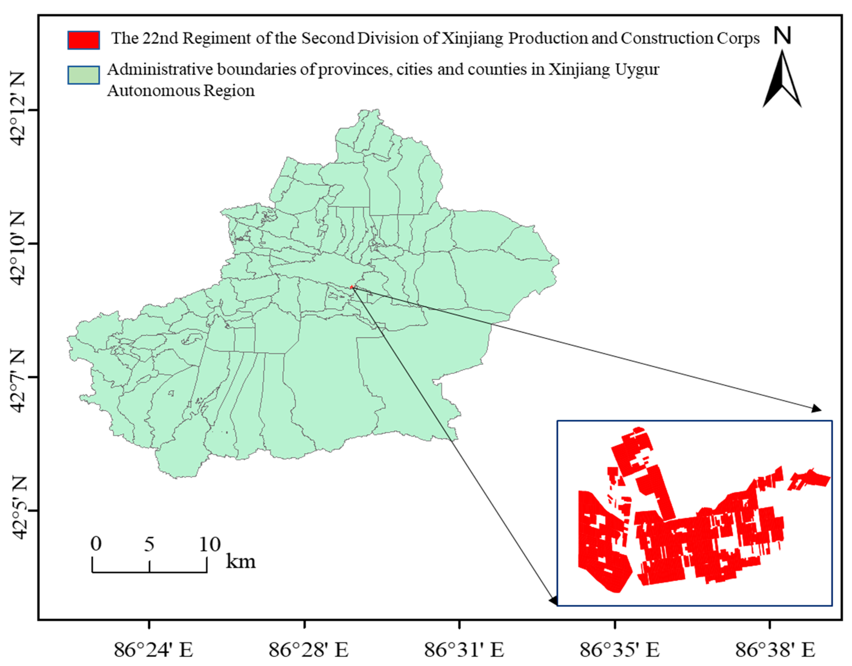
2.1. Study Site

The 22nd Regiment (86°22′–86°48′ N, 42°05′–42°15′ E, a.s.l. 1060–1921 m) is located in the Kaidu River Basin in Xinjiang Uygur Autonomous Region in Central Eurasia (Figure 1). This area has a temperate continental climate, with four distinct seasons, long sunshine duration, large day/night temperature difference, and dry air [31]. The annual average temperature was 8.8 °C, and the average annual precipitation was 59.2 mm. Crops are grown under drip irrigation. The terrain is inclined from northwest to southeast [32]. Soil texture is mainly heavy loam.

2.2. Sampling and Chemical Determination

From April to May 2020, a total of 1853 cultivated lands with an area greater than 33.3 × 10³ m2 were selected in the study area, and five points were selected in each cultivated land along the diagonal for soil sampling (0–20 cm soil layer). The sampling points were positioned using a handheld global positioning system (GPS), with an accuracy of 1–5 m (Garmin eTrex vistah model, Taiwan, China). After removing plant roots, stones, and other impurities, the soil samples of each cultivated land were mixed and paved on a square plastic cloth. Then, a diagonal line was drawn, and one part was discarded. The rest of the soil sample was sealed in polyethylene bags and brought back to the laboratory. In the lab, the soil samples were air-dried, ground, and sieved (0.15 mm and 2 mm).
To determine the soil salinity, a conductivity meter (Shanghai, China DDS-308A) was used to measure the electrical conductivity (EC) of a soil solution (soil:water = 1:5) [33]. Soil organic matter content was determined by potassium dichromate volumetric method, and the soil AN content was determined by alkali hydrolysis diffusion method, soil AP was determined by sodium bicarbonate extraction molybdenum antimony anti colorimetry method, soil AK content was determined by ammonium acetate extraction flame photometer method, and soil Fe, Cu, Mn, and Zn contents were determined by DTPA (diethylene triamine pentacetic acid) using the inductively coupled plasma atomic emission spectrometer (ICP-AES, Leeman labs Inc., Hudson, NH, U.S.A). The above parameters were measured according to the methods of Bao [34]. Each sample was determined for three times, and the average value was calculated.

2.3. Soil Quality Evaluation Criteria

The grading of soil nutrients and heavy metals was based on the Grading Standard of the Second National Soil Census in China [35], and that of soil salinity was based on the Soil Evaluation Grades of Xinjiang [36] (Table 1 and Table 2).

2.3.1. Statistical Analysis

The data of soil salinity, nutrients, and heavy metals were analyzed using the SPSS software (IBM, version 24) to determine the maximum, minimum, average, standard deviation, and coefficient of variation.

2.3.2. Correlation Analysis

To explore the correlation between soil parameters, a correlation matrix between soil parameters was generated using the Origin software (version 2022b). The Pearson correlation coefficient (hereinafter referred to as a p value) was used to describe the quotient of the covariance and standard deviation between two variables (ranging from −1 to 1). The higher the absolute value, the closer the dependence between variables [37].

2.3.3. Analysis of Soil Spatial Variation

The soil evaluation indices were interpolated by the inverse distance weight method (IDW) using ArcGIS software (version 10.6), and the spatial distribution maps for the GCN evaluation results were drawn. IDW is a linear interpolator that evaluates the predicted value of any point based on the assumption of a known dataset [38]. The weighted average was carried out by taking the distance between the interpolation point and the sample point as the weight. The closer the sample point is to the interpolation point, the greater the weight is given. This method is simple, fast, and easy to calculate, and has been widely used to predict unknown values in grids [39].

2.4. Soil Quality Evaluation Methods

2.4.1. Soil Quality Index (SQI)
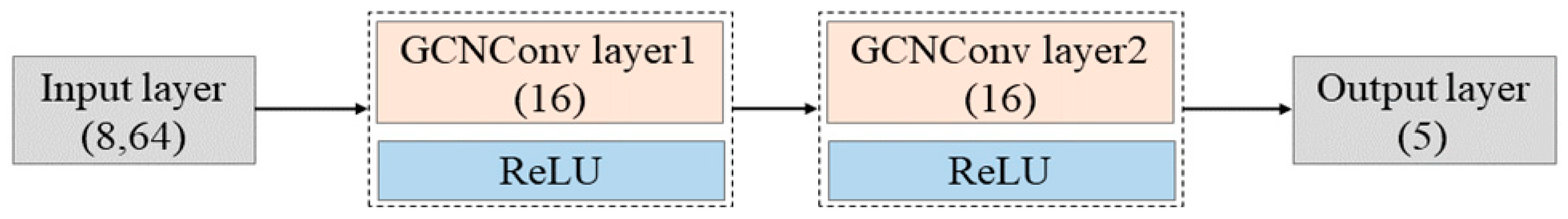
The soil quality index (SQI) integrates the scores of soil quality evaluation indices by calculating the weight and score of each soil quality evaluation index [40].
S Q I = i = 1 n Q ( x i ) Y i
where n is the number of indices, and Q ( x i ) and Y i are the membership degree and weight of the ith index, respectively. The SQI values (0–1.0) were divided into five grades: grade I, 0.8–1.0; grade II, 0.6–0.8; grade III, 0.4–0.6; grade IV, 0.2–0.4; grade V, 0–0.2.
The weight is the ratio of the common factor variance of each index obtained after the principal component analysis to the sum of the common factor variance of all indices.
The type of membership function was determined according to the positive/negative correlation between each index and soil quality variation, and the membership function was used to calculate the membership degree of each index. Function (2) was used for the calculation of the membership degrees of soil nutrients, and Function (3) was used for the calculation of the membership degrees of soil salinity and heavy metals [41].
Q ( x i ) = x i j x i   m i n x i   m a x x i   m i n
Q ( x i ) = x i   m a x x i j x i   m a x x i   m i n
where x i j is the average measured value of each index (SOM, AN, AK, Fe, Cu, Mn, and Zn), x i   m a x is the maximum value of the i th index, and x i   m i n is the minimum value of the i th index.

2.4.2. GCN

GCN is a graph-based neural network. It is essentially a feature extractor acting on topological graph data, which can directly process the graph data of any size and shape, without the limitation of node dissimilarity [42]. In addition, GCN has a good performance in the studies with multiple indicators as inputs. It can directly perform end-to-end learning on the nodes and complete the classification through the nodes and connected edges information in the graph. In a graph where G = (N, E), N represents the nodes and E represents connected edges.
The input of the GCN model includes a feature matrix X (X ∈ Rn×m), adjacency matrix (A ∈ Rn×n), and label group L (L ∈ R2). The X represents the features of all nodes n in the graph, the m represents the dimension of the features of each node, and the A represents the edge connection between nodes in the graph. If there are connected edges between nodes, then A i j = a, where a is the weight of the connected edge, otherwise A i j = 0. The GCN model shows the hidden layer information of the nodes through extracting the adjacent node information, and each layer only captures the information of the nearest neighbor nodes. When the GCN model has multiple layers, the model integrates more neighbor node information. Therefore, the X of the ith hidden layer in the GCN model can be calculated by Formula (4).
H i = f H i 1 , A
where H i = X, and f is the propagation function.
The H i , corresponding to the feature matrix H i R n × k . Here, k represents the dimension of the hidden layer, and n represents the features of a node in the ith layer. The H i R n × k are aggregated to obtain the features of a node in the next hidden layer through the f. For a GCN model with only one hidden layer, the H 1 R n × k of a node can be calculated as follows:
H 1 = ρ ( N ~   ×   W 0 )
N ~ = D 1 2   N   D 1 2
where p is the activation function,   W 0 R m × k is the weight matrix of the 0th layer of the GCN model, and N ~ is the standardized symmetric adjacency matrix in the GCN model.
For multi-layer GCN model, the feature matrix of the next hidden layer H i + 1 can be calculated by the H i and   W i of the previous hidden layer.
H i + 1 = ρ N ~   H i   W i
The GCN structure constructed in this study is shown in Figure 2. The number of nodes in the graph convolution network was 16, the activation layer adopted ReLU, and the one-dimensional data (1 × 8) were converted into a graph of (8, 64) during data input. During model training, Adam was used as the optimizer, the cross-entropy loss was used as the loss function, the learning rate was 0.005, and the number of iterations was 300. The optimal number of layers was determined according to the sparsity of the neighbor node matrix in the graph. When the sparsity is low, then oversmoothing will occur, leading to a low model accuracy when using multiple layers [43]. Additionally, for a simple node classification task, the discrimination of nodes will become worse after using multi-layer GCN, and their vectors tend to be consistent, leading to a series of problems such as gradient disappearance, oversmoothing, and overfitting that obstruct the learning task. In this study, a total of 500 iterations and 5 layers were tested, and it was found that when the number of iterations and layers were 300 and 2, the model accuracy was optimal.

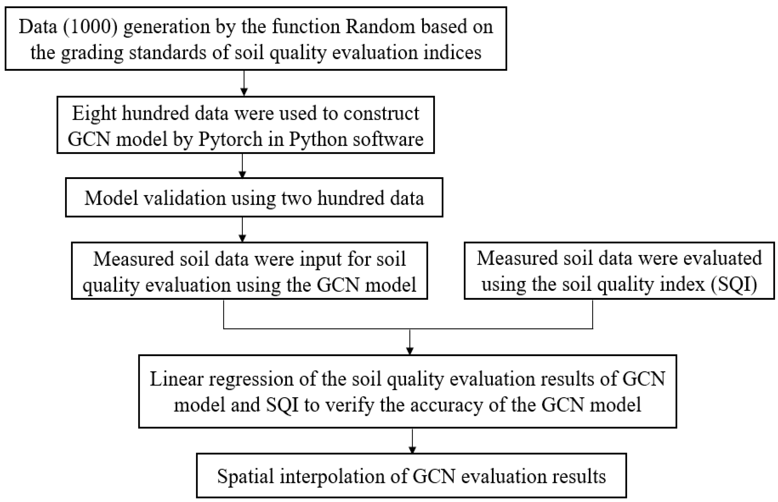
2.4.3. Modeling and Evaluation

Before modeling, soils were graded according to the Grading Standard of the Second National Soil Census in China and the Soil Evaluation Grades of Xinjiang. Because the increase in soil salinity and heavy metal contents will reduce the soil productivity, the soil salinity and heavy metals were evaluated together. To maintain the consistency of the grades of the two grading standards, the soil evaluation grades were regraded (Table 3). Then, the soil quality evaluation model was constructed (Figure 3). (1) According to the soil grading standards, 1000 data (200 per grade) were randomly generated in Python version 3.8. (2) Eighty percent of the data were randomly selected for network training based on GCN, and the rest of the data were used as the validation set for model validation. (3) The measured soil data (soil nutrients, soil salinity, and heavy metals) (Table 3) were input into the GCN model, and then the soil grading results (I, II, III, IV, V) were automatically output. (4) The soil grading results by SQI were linearly fitted to the soil grading results by GCN to evaluate the model accuracy, and then the spatial interpolation of the evaluation results by GCN was performed.
In this study, the confusion matrix was used to determine the GCN model evaluation accuracy. The confusion matrix is suitable for the statistics of data classification accuracy, and it can accurately and objectively evaluate the overall distribution and change trend of features. The confusion matrix accuracy refers to the percentage of correctly predicted samples in the total sample. The larger the element value on the diagonal on the confusion matrix, the higher the reliability of the classification results. Conversely, the larger the element value on the non-diagonal, the more serious the misclassification [44].

3. Results

3.1. Statistical Analysis of the Values of Soil Quality Evaluation Indices

Soil salinity was 0.2–26.6 g/kg in the study area, and the average value was 5.25 g/kg (Grade V). The average contents of SOM, AN, AK, Fe, Cu, Mn, and Zn were 18.59 g/kg (Grade IV), 72.86 mg/kg (Grade IV), 188.78 mg/kg (Grade II), 17.33 mg/kg (Grade II), 3.08 mg/kg (Grade I), 7 mg/kg (Grade III), and 1.3 mg/kg (Grade II), respectively (Table 4). The coefficients of variation of these indices were in the range of 20–86%, indicating a medium variation. Among the indices, salinity had the largest variation (86%), while SOM had the smallest variation (20%).
For soil salinity, the number of Grade V soil samples was the largest, accounting for 63.9%, and that of Grade III was the least, accounting for 4.7%. For SOM and AN, the number of Grade IV soil samples were the largest, accounting for 69.2% and 45.8%, respectively. For AK, the number of Grade I soil samples was the largest (34.8%), followed by the Grade II and Grade III. For Fe, the number of Grade II soil samples was the largest, accounting for 46.8%. For Cu, the number of Grade I soil samples was the largest, accounting for 97.9%. For Mn, the number of Grade IV soil samples was the largest, accounting for 51.2%. For Zn, the number of Grade III soil samples was the largest, accounting for 47% (Table 5).

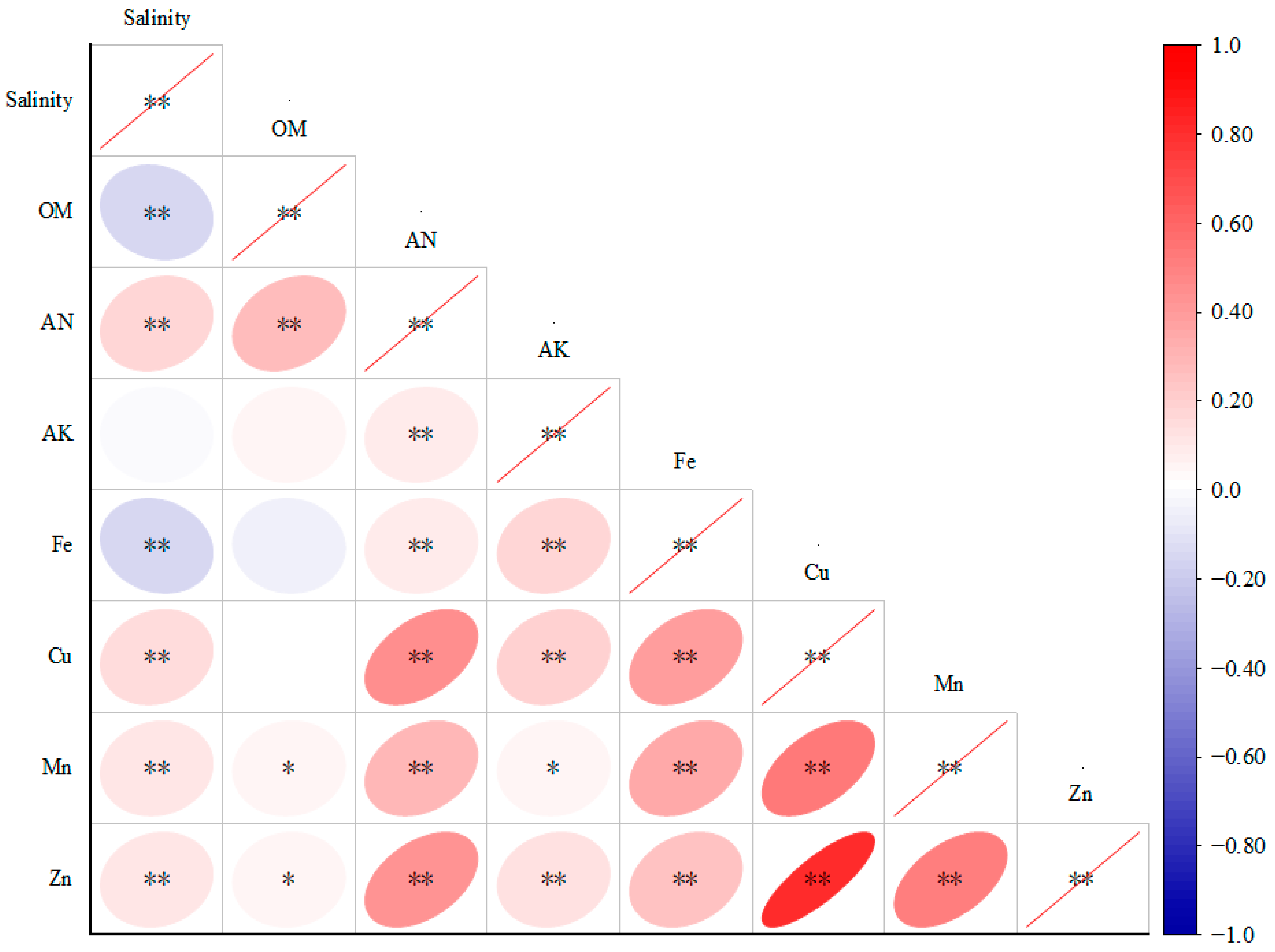
3.2. Correlation Analysis of Soil Evaluation Indices

Pearson correlation analysis showed (Figure 4) that soil salinity was negatively correlated with SOM and Fe (p < 0.01), and positively correlated with the indices except for AK, OM, and Fe (p < 0.05). SOM was positively correlated with AN (p < 0.01), Mn (p < 0.05), and Zn (p < 0.05). AN was positively correlated with all indices (p < 0.01). AK was positively correlated with Fe (p < 0.01), Cu (p < 0.01), Zn (p < 0.01), and Mn (p < 0.05). Fe was negatively correlated with salinity (p < 0.01) and SOM (p > 0.05), and positively correlated with other indices (p < 0.01). Cu was positively correlated with all indices except SOM (p < 0.01). Mn was positively correlated with SOM (p < 0.05), AK (p < 0.05), and other indices (p < 0.01). Zn was positively correlated with SOM (p < 0.05) and negatively correlated with other indices (p < 0.01). There was a positive correlation between soil heavy metals (p < 0.01).

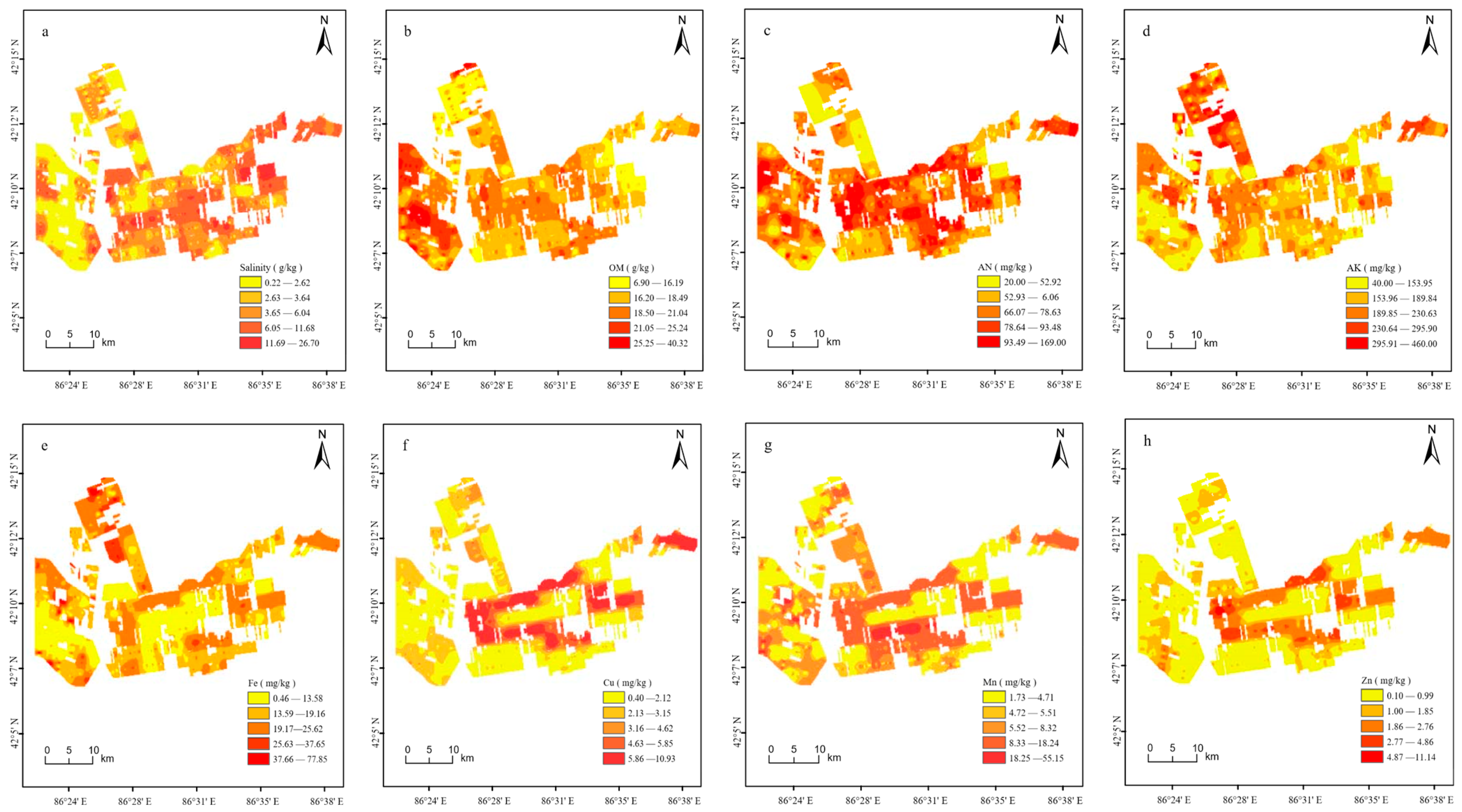
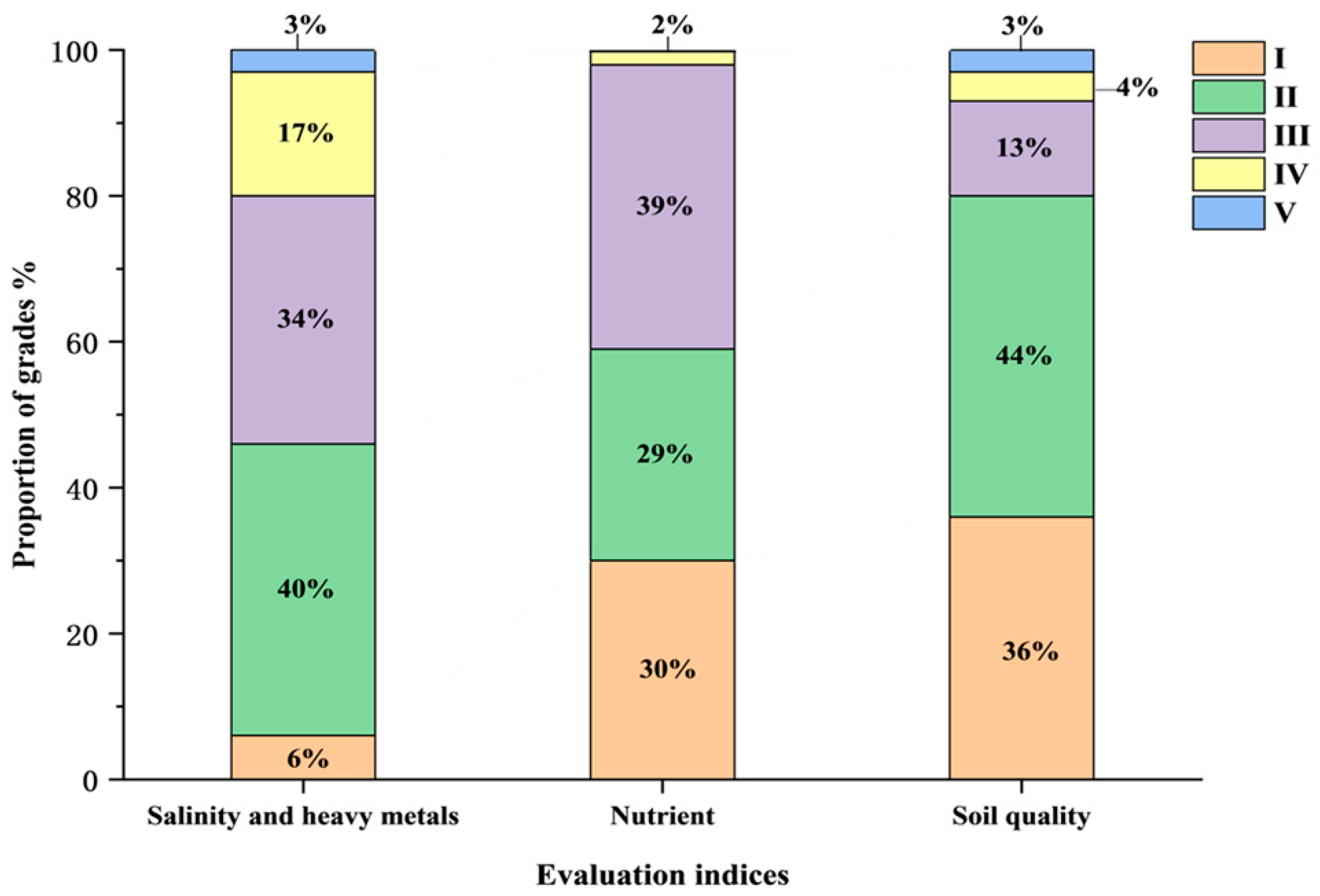
3.3. Spatial Variation of Soil Samples of Different Grades
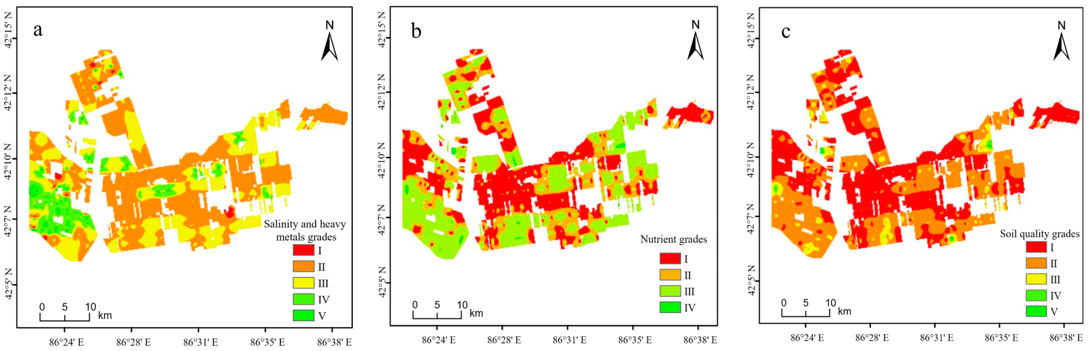
Soil salinity was high in the central, eastern, and southern regions, and low in the western region (Figure 5a). The SOM content was high in the western region and low in the northern and eastern regions (Figure 5b). AN was high in the western and central regions (Figure 5c). The number of soil samples with a high AK content was low, which were mainly distributed in the northern region (Figure 5d). Soil salinity gradually increased from west to east, while soil nutrient contents gradually decreased. Fe was high in the northern region and low in the western and central regions (Figure 5e). The soil samples with high Cu, Mn, and Zn contents were mainly concentrated in the central region (Figure 5f–h).

3.4. SQI Evaluation

The SQI evaluation results showed that soil salinity/heavy metals (SQI value: 0.18–0.94, average: 0.78) was at Grade II, soil nutrients (SQI value: 0.02–0.68, average: 0.35) was at Grade IV, and soil quality (SQI value: 0.19–0.83, average: 0.67) was at Grade II (Table 6).

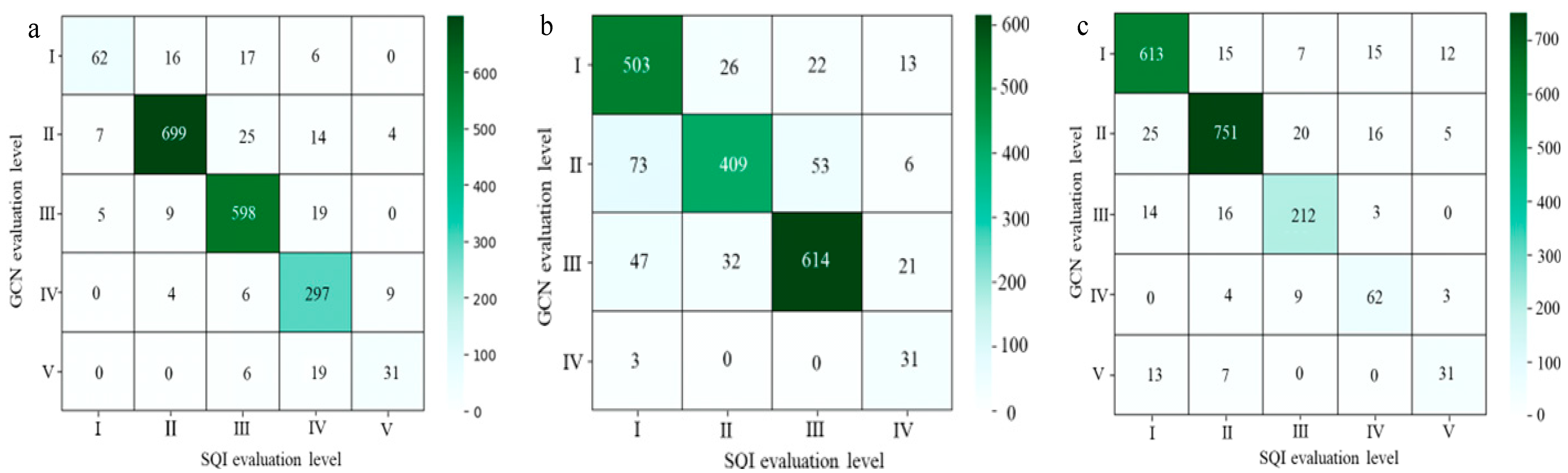
3.5. GCN Model Evaluation

For soil salinity/heavy metals, Grade V soil samples accounted for the least (3%), Grade I soil samples accounted for 6% of the total, and Grades I and V soil samples were mainly distributed in the western and northern regions. Grade II soil samples were the most (40%), concentrated in the central region. Grade III soil samples accounted for 34%, and were dispersedly distributed in the study area. Grade IV soil samples accounted for 17%, concentrated in the western region (Figure 6 and Figure 7a).
For soil nutrients, Grade I soil samples accounted for 30%, mainly concentrated in the central region. Grade II soil samples accounted for 29%, distributed around Grade I soil samples. Grade III soil samples represented the largest group (39%), mainly distributed in the southwest region. Grade IV soil samples were the smallest (2%), distributed in the western and eastern regions (Figure 6 and Figure 7b).
For soil quality, Grade I soil samples accounted for 36%, concentrated in the central region. Grade II soil samples were the largest (44%). Grade III soil samples accounted for 13%, scattered across the study area. Grade IV and V soils accounted for 4% and 3%, respectively, distributed in the western, eastern, and southern regions (Figure 6 and Figure 7c).
The confusion matrix (Figure 8) showed that Grade II had the highest accuracy in the soil salinity/heavy metals evaluation results, followed by Grades III, IV, I, and V. Grade III had the highest accuracy in the soil nutrient evaluation results, and Grade IV had the lowest accuracy. Grade II had the highest accuracy in the soil quality evaluation results, and Grade V had the lowest accuracy. The evaluation accuracy of the GCN model for soil salinity/heavy metals, soil nutrients, and soil quality were 0.91, 0.84, and 0.90, respectively. Therefore, the GCN model had a high evaluation accuracy.

4. Discussion

4.1. Analysis of Soil Quality Evaluation Indices

The soil salinity of the cotton fields in the study area was at a very low level (Grade V) (Table 4), indicating a low degree of salinization in the study area. This is consistent with the study results obtained by Liu et al. [45]. This may be due to the fact that the widely applied drip irrigation could desalt the plough layer by eluviation [46]. The content of most soil nutrients were at a medium level, but the soil AK content was high. This may be due to the fact that soil is rich in potassium in Xinjiang [47]. Although some soil potassium is absorbed by crops, potassium is supplemented by fertilization, which thus maintains the potassium content at a high level. Although the content of the soil heavy metals was lower than the background value of Xinjiang, it was still high (Table 4). This may be due to the fact that the discharge of the industrial and agricultural wastewater increases the heavy metals in the Bosten Lake [48]. Then, the long-time use of water to irrigate cotton fields ultimately increases the content of the soil heavy metals [49].
This study found that soil evaluation indices were in medium variation (Table 4). The coefficient of variation of salinity was the highest. This indicates the obvious spatial heterogeneity of the soil salinity [50]. This may be caused by differences in soil type and soil texture [51]. For example, the finer the soil texture, the more conducive it is to the accumulation of salt. Additionally, it may also be related to difference in agricultural managements. For example, although drip irrigation is widely adopted in the study area, some areas still adopt flood irrigation. However, flood irrigation can easily raise the groundwater level, and lead to increased surface salinity. Additionally, the excessive application of nitrogen fertilizer can also accelerate soil salinization [52]. The coefficient of variation of soil nutrients was lower than other indices. This may be related to the unified irrigation and fertilization. Drip irrigation is conducive to improving the uniformity of irrigation. Moreover, fertilization through the drip irrigation system promotes the homogenization of surface soil nutrients [53]. The coefficients of variation of soil heavy metals were generally higher than those of soil nutrients. This may be due to the fact that farmlands along Bosten Lake are irrigated with lake water [54].
The correlation analysis results showed that soil salinity had a correlation with SOM, AN, and heavy metals (p < 0.01) (Figure 4). This indicates that soil salinization and soil heavy metal pollution may jointly affect the cultivated lands in the study area. This may be related to the soil texture and irrigation using Bosten Lake water [55]. Additionally, soil salinity is closely related to the transformation of SOM, AN, and heavy metal forms, which further affects the distribution and migration of nutrients and heavy metals in the soil [56]. This study also found that there was a positive correlation between heavy metals, especially Cu and Zn (p < 0.01). This indicates that there is multi-heavy metal pollution in cotton fields in the study area, and the homology between heavy metals is high. The high content of heavy metals in the soil is closely related to the long-term application of chemical fertilizers and the long-term use of Bosten Lake water for irrigation.

4.2. Spatial Distribution Characteristics of Soils of Different Grades

Xinjiang is in an arid area. The spatial distribution and conversion of soils of different quality in the cotton fields are the result of the joint action of structural factors and random factors. In the study area, the uneven patch size and irregular distribution are the spatial distribution characteristics of soils of different grades. This may be related to the micro-topography and soil parent materials [57,58]. It was found that soil salinity gradually increased from west to east in the study area, while the soil nutrient contents gradually decreased. This may be related to the terrain. The study area is crossed by two branches of Bosten Lake, namely the Huangshuigou River in the northwest and the Kaidu River in the southwest. The adequate groundwater affects plant diversity as well as the soil microbial community, which indirectly affects the soil nutrient contents [59]. Additionally, because water can regulate the cycle of nitrogen and promote the storage of SOM and AN, the adequate water can indirectly increase soil nutrient contents [60]. The distribution law of AN may be related to the C/N ratio of SOM [61].
Heavy metal content is an important indicator of soil quality [62]. The content of heavy metals in soil is not only affected by a variety of environmental factors, but is also related to the cropping system, fertilization, and other human activities [63]. In this study, soil heavy metals showed a similar spatial distribution in the study area. This indicates that soil heavy metals have a common source. Additionally, the soil heavy metal content was high in the central region. This may be related to the soil parent material [64]. The area with high soil heavy metal contents is between the Huangshuigou River and the Kaidu River. The rivers brings massive fluvial sediments, which affects the content and spatial distribution of soil heavy metals [65]. On the other hand, it may be caused by human factors. Human activities are more and more frequent, especially the development of industry and agriculture, which may increase the content of heavy metals in soil as well as result in large differences in soil heavy metals in some areas [66]. For example, wastewater is used in some areas to irrigate farmlands, leading to soil pollution and degradation [67].

4.3. Soil Quality Evaluation Based on GCN Model

The GCN model evaluation results were highly consistent with those of SQI (Table 6, Figure 6). Soil salinity/heavy metals were evaluated at Grade II by the GCN model and SQI. Soil nutrients were evaluated at Grade IV and III by the SQI and GCN model, respectively. This difference may be due to the fact that the relatively fewer evaluation parameters of soil nutrients resulted in fewer new node features extracted by GCN and poor identification. Soil quality was evaluated at Grade II by SQI and GCN. The accuracy of the GCN model evaluated by the confusion matrix showed that the GCN model had a high accuracy in evaluating soil salinity/heavy metals (0.90), soil nutrients (0.84), and soil quality (0.91) (Figure 8). The traditional method (SQI) involves cumbersome calculations, low efficiency, low speed, and difficulty in processing a large amount of soil data in batches. However, the GCN model has a fast running speed, simple operation, high efficiency, and high accuracy. Therefore, the use of GCN in the evaluation of soil quality is feasible.
Additionally, the data of the complex soil have a complex nonlinear relationship. The GCN can clarify the nonlinear relationship between soil parameters, highlight the soil characteristics and information on the associated nodes in the soil data structure, and extract hidden and weak soil features. Therefore, the GCN can fully express the soil data structure. Additionally, the calculation of the next layer of features of each node is only related to itself and its neighbor nodes in the GCN, so GCN is a kind of local structure connection. This effectively reduces the computational complexity, making this method simple and efficient. However, for the traditional method SQI, it is first necessary to calculate the weight of each index, and then calculate the membership degree of each index, followed by the addition of a formula to obtain the soil quality index. Therefore, SQI is more complicated and cumbersome.
The spatial distribution analysis results (Figure 7) showed that there was a certain relationship between the soil heavy metals and the soil nutrients and between soil heavy metals and soil salinity. Especially in areas with high human activity intensity, soil nutrients are rich, the soil salinity is low, but soil heavy metals are high. Farmers in Xinjiang adopt deep tillage to improve the soil structure and plastic film mulching to improve the soil permeability, inhibit soil water evaporation, and reduce salt accumulation [68]. The differences in soil nutrients and heavy metals in different areas may be related to differences in human activity intensities and agriculture management [69]. In some areas, excessive fertilization or irrigation with alkaline water has led to soil nutrient imbalance.
According to the soil quality evaluation results by the GCN model, this study puts forward some fertilization suggestions. Although the soil quality is at Grade II as a whole in the study area, the soil quality in some areas remains poor. Therefore, fertilization based on soil testing should be adopted, and organic fertilizers and straw return can be adopted to supplement SOM and reduce soil salinity. Additionally, soil heavy metals are generally high and unevenly distributed. Therefore, fertilization using chemical fertilizers and irrigation using polluted water should be restricted. Crop rotation and stubble retention can be adopted to reduce the soil heavy metals and improve the soil quality.

5. Conclusions

In this study, GCN was used to evaluate the soil quality (soil nutrients, salinity, and heavy metals) by transforming the soil quality grading into a nonlinear issue. The GCN can extract the irregular characteristics of graph data and the rules of evaluation indices, which improves the operational efficiency and the objectivity and accuracy of evaluation results. Therefore, this method can be used in soil quality evaluation. This study will provide a reference for scientific fertilization and soil quality management in arid areas. The main conclusions are as follows:
In the study area, the soil salinity was evaluated at grade V (average value: 5.25 g/kg), the SOM and AN contents were evaluated at grade IV (average value: 18.59 mg/kg and 72.86 mg/kg, respectively), and the AK content was evaluated at grade II (average value: 188.78 mg/kg). The soil heavy metal content was generally high. The coefficients of variation of the evaluation indices were 20–86%, i.e., there was a large variation, among which soil salinity variation was the largest (86%) and SOM variation was the smallest (20%). From the perspective of spatial distribution, soil salinity gradually increased from west to east, while the soil nutrient content gradually decreased. The Fe content was high in the northern region and low in the western and central regions. Soil samples with a higher Cu, Mn, and Zn content were mainly distributed in the central region. Therefore, the spatial distributions of soil heavy metals were similar. Additionally, there was a positive correlation between soil salinity and SOM, AN, and heavy metals (p < 0.01) as well as between Cu and Zn (p < 0.01). Based on the spatial distribution and correlation analysis results, it was concluded that there was high homology between the soil salinity and heavy metals as well as between heavy metals.
The overall evaluation results of the GCN model and SQI were highly consistent. Soil salinity/heavy metals were evaluated at Grade III, and the Grade III soils were mainly distributed in the central region. The soil nutrient evaluation results were similar (Grade III by SQI and Grade IV by GCN), and the areas with high grades were mainly concentrated in the central region. The overall soil quality was evaluated at Grade II by GCN and SQI. The spatial distribution of soils with high-grade soil salinity/heavy metals, soil nutrients, and soil quality were very similar. The evaluation accuracy of the GCN model for soil salinity/heavy metals, soil nutrients, and soil quality were 0.91, 0.84, and 0.90, respectively. Therefore, the GCN model shows a good evaluation performance. It has a fast operation, simple operation, high efficiency, and high evaluation accuracy. It has great potential in practical application.
In this study, the GCN model was used to evaluate the soil salinity/heavy metals, soil nutrients, and soil quality. These indicators are limited. Therefore, in our future studies, more indicators will be added, such as soil physical indicators (soil bulk density, soil moisture, etc.), soil biological indicators (catalase, protease, biodiversity, etc.), remote sensing data (band, vegetation index), and environmental covariates (rainfall, altitude, slope, temperature), to improve the accuracy of soil quality evaluation, explore the contribution of different variables to soil quality evaluation, and determine the main variables affecting soil quality in this area. In addition, this method is a comprehensive evaluation index, which can be tried to be applied to water pollution and vegetation growth in the future. For example, pH, heavy metals, organophosphorus, sulfide, and other indicators can be used to construct a comprehensive water pollution evaluation index based on GCN; leaf area, biomass, yield, plant height, and other indicators can be used to construct a comprehensive vegetation growth evaluation index based on GCN, to verify the performance of the GCN method in the evaluation of water pollution and vegetation growth, and explore the versatility of the GCN method. Finally, the GCN model constructed in this study has limitations in network depth. We will increase the network depth in the future or optimize GCN through other networks to improve the stability and versatility of the GCN model.

Author Contributions

Conceptualization, X.F. and X.L.; methodology, X.F. and P.G.; software, M.Z.; validation, Z.Z., L.Z. (Li Zuo) and Q.Z.; formal analysis, Q.Z. and H.C.; investigation, L.Z. (Li Zuo); resources, X.L.; data curation, L.Z. (Lifu Zhang); writing—original draft preparation, X.F.; writing—review and editing, X.F.; visualization, L.D.; supervision, X.L.; project administration, X.L.; funding acquisition, X.L. All authors have read and agreed to the published version of the manuscript.

Funding

This study was supported by the Leading Talent Project of the Talent Support Plan of Xinjiang Production and Construction Corps (20230057102).

Data Availability Statement

The data presented in this study are available on request from the corresponding author.

Conflicts of Interest

The authors declare no conflict of interest.

References

  1. Mi, W.; Sun, T.; Ma, Y.; Chen, C.; Ma, Q.; Wu, L.; Wu, Q.; Xu, Q. Higher Yield Sustainability and Soil Quality by Manure Amendment than Straw Returning under a Single-Rice Cropping System. Field Crop. Res. 2023, 292, 108805. [Google Scholar] [CrossRef]
  2. Kurmangozhinov, A.; Xue, W.; Li, X.; Zeng, F.; Sabit, R.; Tusun, T. High biomass production with abundant leaf litterfall is critical to ameliorating soil quality and productivity in reclaimed sandy desertification land. J. Environ. Manag. 2020, 263, 110373. [Google Scholar] [CrossRef] [PubMed]
  3. Liu, X.; Meng, L.; Yin, T.; Wang, X.; Zhang, S.; Cheng, Z.; Ogundeji, A.O.; Li, S. Maize/soybean intercrop over time has higher yield stability relative to matched monoculture under different nitrogen-application rates. Field Crop. Res. 2023, 301, 109015. [Google Scholar] [CrossRef]
  4. Lowe, M.-A.; Mathes, F.; Loke, M.H.; McGrath, G.; Murphy, D.V.; Leopold, M. Bacillus Subtilis and Surfactant Amendments for the Breakdown of Soil Water Repellency in a Sandy Soil. Geoderma 2019, 344, 108–118. [Google Scholar] [CrossRef]
  5. Zheng, L.; Jiang, C.; Chen, X.; Li, Y.; Li, C.; Zheng, L. Combining hydrochemistry and hydrogen and oxygen stable isotopes to reveal the influence of human activities on surface water quality in Chaohu Lake Basin. J. Environ. Manag. 2022, 312, 114933. [Google Scholar] [CrossRef]
  6. Santos-Francés, F.; Martínez-Graña, A.; Ávila-Zarza, C.; Criado, M.; Sánchez, Y. Comparison of methods for evaluating soil quality of semiarid ecosystem and evaluation of the effects of physico-chemical properties and factor soil erodibility (Northern Plateau, Spain). Geoderma 2019, 354, 113872. [Google Scholar] [CrossRef]
  7. Wang, Z.; Jin, M.; Šimůnek, J.; van Genuchten, M.T. Evaluation of mulched drip irrigation for cotton in arid Northwest China. Irrig. Sci. 2014, 32, 15–27. [Google Scholar] [CrossRef]
  8. Han, C.; Zheng, J.; Guan, J.; Yu, D.; Lu, B. Evaluating and Simulating Resource and Environmental Carrying Capacity in Arid and Semiarid Regions: A Case Study of Xinjiang, China. J. Clean. Prod. 2022, 338, 130646. [Google Scholar] [CrossRef]
  9. Wu, C.; Liu, G.; Huang, C.; Liu, Q. Soil quality assessment in Yellow River Delta: Establishing a minimum data set and fuzzy logic model. Geoderma 2019, 334, 82–89. [Google Scholar] [CrossRef]
  10. Han, Z.G.; Chen, H.; Cao, Y.W.; He, L.; Si, Z.F.; Hu, Y.; Lin, H.; Ning, X.Z.; Li, Q.M.; Liu, F.J.; et al. Genomic insights into genetic improvement of upland cotton in the world’s largest growing region. Ind. Crop. Prod. 2022, 183, 114929. [Google Scholar] [CrossRef]
  11. Li, C.B.; Xiao, K.Y.; Li, N.; Song, X.L.; Zhang, S.; Wang, K.; Chu, W.K.; Cao, R. A comparative study of support vector machine, random forest and artificial neural network machine learning algorithms in geochemical anomaly information extraction. Acta Geosci. Sinica. 2020, 2, 309–319, (In Chinese with English Abstract). [Google Scholar] [CrossRef]
  12. Essa, F.A.; Elaziz, M.A.; Elsheikh, A.H. An enhanced productivity prediction model of active solar still using artificial neural network and Harris Hawks optimizer. Appl. Therm. Eng. 2020, 170, 115020. [Google Scholar] [CrossRef]
  13. Zhang, D.Y.; Zhang, W.; Huang, W.; Hong, Z.M.; Meng, L.K. Upscaling of surface soil moisture using a deep learning model with VIIRS RDR. ISPRS. Int. J. Geo-Inf. 2017, 6, 130. [Google Scholar] [CrossRef]
  14. Bruna, J.; Zaremba, W.; Szlam, A.; Le, C.Y. Spectral networks and locally connected networks on graphs. arXiv 2014, arXiv:1312.6203. [Google Scholar] [CrossRef]
  15. Fukunaga, I.; Sawada, R.; Shibata, T.; Kaitoh, K.; Sakai, Y.; Yamanishi, Y. Prediction of the health effects of food peptides and elucidation of the mode-ofaction using multi-task graph convolutional neural network. Mol. Inform. 2020, 39, 1900134. [Google Scholar] [CrossRef]
  16. Ramirez, R.; Chiu, Y.C.; Hererra, A.; Mostavi, M.; Ramirez, J.; Chen, Y.; Huang, Y.; Jin, Y.F. Classification of Cancer Types Using Graph Convolutional Neural Networks. Front. Phys. 2020, 8, 203. [Google Scholar] [CrossRef]
  17. Zhou, J.; Cui, G.; Hu, S.; Zhang, Z.; Yang, C.; Liu, Z.; Wang, L.; Li, C.; Sun, M. Graph neural networks: A review of methods and applications. AI Open 2020, 1, 57–81. [Google Scholar] [CrossRef]
  18. Wu, Z.; Chen, H.; Zhang, J.; Liu, S.; Huang, R.; Pei, Y. A directed link prediction method using graph convolutional network based on social ranking theory. Intell. Data Anal. 2021, 25, 739–757. [Google Scholar] [CrossRef]
  19. Wu, Z.; Pan, S.; Chen, F.; Long, G.; Zhang, C.; Yu, P.S. A Comprehensive Survey on Graph Neural Networks. IEEE Trans. Neural Netw. Learn. Syst. 2021, 32, 4–24. [Google Scholar] [CrossRef]
  20. Zhao, D.; Wang, J.; Lin, H.; Yang, Z.; Zhang, Y. Extracting drug–drug interactions with hybrid bidirectional gated recurrent unit and graph convolutional network. J. Biomed. Inform. 2019, 99, 103295. [Google Scholar] [CrossRef]
  21. Shi, J.; Wang, R.; Zheng, Y.; Jiang, Z.; Yu, L. Cervical cell classification with graph convolutional network. Comput. Meth. Prog. Bio. 2021, 198, 105807. [Google Scholar] [CrossRef] [PubMed]
  22. Bin, Y.; Chen, Z.M.; Wei, X.S.; Chen, X.; Gao, C.; Sang, N. Structure-aware human pose estimation with graph convolutional networks. Pattern Recognit. 2020, 106, 107410. [Google Scholar] [CrossRef]
  23. Zhao, G.; He, H.; Huang, Y.; Ren, J. Near-surface PM2.5 prediction combining the complex network characterization and graph convolution neural network. Neural Comput. Appl. 2021, 33, 17081–17101. [Google Scholar] [CrossRef]
  24. Abdel-Fattah, M.K.; Mohamed, E.S.; Wagdi, E.M.; Shahin, S.A.; Aldosari, A.A.; Lasaponara, R.; Alnaimy, M.A. Quantitative Evaluation of Soil Quality Using Principal Component Analysis: The Case Study of El-Fayoum Depression Egypt. Sustainability-basel. 2021, 13, 1824. [Google Scholar] [CrossRef]
  25. Qin, S.; Xu, Y.; Liu, H.; Li, C.; Yang, Y.; Zhao, P. Effect of different boron levels on yield and nutrient content of wheat based on grey relational degree analysis. Acta Physiol. Plant 2021, 43, 127. [Google Scholar] [CrossRef]
  26. Peng, M.; He, H.; Wang, Z.; Li, G.; Lv, X.; Pu, X.; Zhuang, L. Responses and comprehensive evaluation of growth characteristics of ephemeral plants in the desert–oasis ecotone to soil types. J. Environ. Manag. 2022, 316, 115288. [Google Scholar] [CrossRef]
  27. Huang, Y.; Chen, Q.; Deng, M.; Japenga, J.; Li, T.; Yang, X.; He, Z. Heavy metal pollution and health risk assessment of agricultural soils in a typical peri-urban area in southeast China. J. Environ. Manag. 2018, 207, 159–168. [Google Scholar] [CrossRef]
  28. Sharma, K.; Janardhana Raju, N.; Singh, N.; Sreekesh, S. Heavy metal pollution in groundwater of urban Delhi environs: Pollution indices and health risk assessment. Urban Clim. 2022, 45, 101233. [Google Scholar] [CrossRef]
  29. Della Chiesa, S.; La Cecilia, D.; Genova, G.; Balotti, A.; Thalheimer, M.; Tappeiner, U.; Niedrist, G. Farmers as data sources: Cooperative framework for mapping soil properties for permanent crops in South Tyrol (Northern Italy). Geoderma 2019, 342, 93–105. [Google Scholar]
  30. Lei, K.; Li, Y.; Zhang, Y.; Wang, S.; Yu, E.; Li, F.; Xiao, F.; Xia, F. Development of a New Method Framework to Estimate the Nonlinear and Interaction Relationship between Environmental Factors and Soil Heavy Metals. Sci. Total. Environ. 2023, 905, 167133. [Google Scholar] [CrossRef]
  31. Li, C.M.; Ma, Y.Z.; Xu, W.X.; Wang, F.; Li, P.C.; Li, L.; Fang, Y.F.; Zhang, N. Effects of different nitrogen application rates on cotton yield and soil nutrients in cotton fields. J. Agr. Sci. 2022, 36, 1446–1455. [Google Scholar] [CrossRef]
  32. Wang, J.; Peng, J.; Li, H.; Yin, C.; Liu, W.; Wang, T.; Zhang, H. Soil Salinity Mapping Using Machine Learning Algorithms with the Sentinel-2 MSI in Arid Areas, China. Remote Sens. 2021, 13, 305. [Google Scholar] [CrossRef]
  33. Scudiero, E.; Skaggs, T.H.; Corwin, D.L. Simplifying field-scale assessment of spatiotemporal changes of soil salinity. Sci. Total. Environ. 2017, 587, 273–281. [Google Scholar] [CrossRef] [PubMed]
  34. Bao, S.D. Soil Agrochemical Analysis; China Agricultural Press: Beijing, China, 2000; p. 1. [Google Scholar]
  35. Zhang, F.S. Essentials of Soil Testing and Formula Fertilization Technology; China Agricultural University Press: Beijing, China, 2006. [Google Scholar]
  36. Zheng, Q. Comprehensive Evaluation of Soil Environmental Quality of Cotton Field in Xinjiang Oasis. Master’s Thesis, Shihezi University, Shihezi, China, 2018. [Google Scholar] [CrossRef]
  37. Bermudez-Edo, M.; Barnaghi, P.; Moessner, K. Analysing real world data streams with spatio-temporal correlations: Entropy vs. Pearson correlation. Autom. Constr. 2018, 88, 87–100. [Google Scholar] [CrossRef]
  38. Li, Z. An enhanced dual IDW method for high-quality geospatial interpolation. Sci. Rep. 2021, 11, 9903–9917. [Google Scholar] [CrossRef]
  39. Oliveira, J.A.J.D.; Souza, S.R.L.D.; Dal, P.E.; Rodrigues, B.T.; Souza, V.C.D. Aurora: Mobile application for analysis of spatial variability of thermal comfort indexes of animals and people, using IDW interpolation. Comput. Electron. Agr. 2019, 157, 98–101. [Google Scholar] [CrossRef]
  40. Zeraatpisheh, M.; Bakhshandeh, E.; Hosseini, M.; Alavi, S.M. Assessing the effects of deforestation and intensive agriculture on the soil quality through digital soil mapping. Geoderma 2020, 363, 114139. [Google Scholar] [CrossRef]
  41. Wen, X.; Hong, M.; Zhang, Y.X.; Pei, Z.F.; Zhao, H.X.; Chen, C. Effects of organic materials addition on the organic carbon pool and soil quality of alkalized soil. Chin. J. Grassl. 2022, 44, 39–49. [Google Scholar] [CrossRef]
  42. Yu, B.; Lee, Y.; Sohn, K. Forecasting road traffic speeds by considering area-wide spatio-temporal dependencies based on a graph convolutional neural network (GCN). Transp. Res Part C-Emer. 2020, 114, 189–204. [Google Scholar] [CrossRef]
  43. Song, Y.; Lu, S.; Qiu, D. Improving Node Classification through Convolutional Networks Built on Enhanced Message-Passing Graph. Comput. Intel. Neurosc. 2022, 2022, e3999144. [Google Scholar] [CrossRef]
  44. Pang, P.S.; Hou, X.; Xia, L. Borrowers’ credit quality scoring model and applications, with default discriminant analysis based on the extreme learning machine. Technol. Forecast. Soc. 2021, 165, 120462. [Google Scholar] [CrossRef]
  45. Liu, X.H.; Bai, Y.G.; Chai, Z.P.; Zhang, J.H.; Jiang, Z.; Ding, B.X.; Zhang, C. Multispectral remote sensing inversion and seasonal difference in soil salinity of cotton field in typical oasis irrigation area. J. Agric. Resour. Environ. 2023, 40, 598–609. [Google Scholar]
  46. Wei, X.; Huang, S.; Huang, Q.; Liu, D.; Leng, G.; Yang, H.; Duan, W.; Li, J.; Bai, Q.; Peng, J. Analysis of Vegetation Vulnerability Dynamics and Driving Forces to Multiple Drought Stresses in a Changing Environment. Remote Sens. 2022, 14, 4231. [Google Scholar] [CrossRef]
  47. Zhu, S.; Lei, Y.; Wang, C.; Wei, Y.; Wang, C.; Sun, Y. Patterns of yeast diversity distribution and its drivers in rhizosphere soil of Hami melon orchards in different regions of Xinjiang. BMC Microbiol. 2021, 21, 170. [Google Scholar] [CrossRef]
  48. Wei, G.Y. Ecological Changes and Possible Mechanisms of Alpine-Oasis Lakes in the Arid Region of Northwest China in the Past Two Thousands of Years. Master’s Thesis, Lanzhou University, Lanzhou, China, 2018. [Google Scholar]
  49. Wen, X.; Lu, J.; Wu, J.; Lin, Y.; Luo, Y. Influence of coastal groundwater salinization on the distribution and risks of heavy metals. Sci. Total. Environ. 2019, 652, 267–277. [Google Scholar] [CrossRef]
  50. Niu, F.P.; Li, X.G.; Jin, W.G.; Mai, M.T.T.R.X.E.Z.Z. Characteristics of soil salinity in the western lakeside oasis of Bosten Lake. Soil. Fertil. Sci. China 2020, 3, 8–15. [Google Scholar] [CrossRef]
  51. Yu, Y.; Zhao, C.; Zheng, N.; Jia, H.; Yao, H. Interactive effects of soil texture and salinity on nitrous oxide emissions following crop residue amendment. Geoderma 2019, 337, 1146–1154. [Google Scholar] [CrossRef]
  52. Che, Z.; Wang, J.; Li, J. Determination of threshold soil salinity with consideration of salinity stress alleviation by applying nitrogen in the arid region. Irrig. Sci. 2022, 40, 283–296. [Google Scholar] [CrossRef]
  53. Surendran, U.; Madhava, C.K. Development and evaluation of drip irrigation and fertigation scheduling to improve water productivity and sustainable crop production using HYDRUS. Agr. Water Manag. 2022, 269, 107668. [Google Scholar] [CrossRef]
  54. Mamat, Z.; Haximu, S.; Zhang, Z.Y.; Aji, R. An ecological risk assessment of heavy metal contamination in the surface sediments of Bosten Lake, northwest China. Environ. Sci. Pollut. Res. 2016, 23, 7255–7265. [Google Scholar] [CrossRef]
  55. Chen, L.; Wei, Q.; Xu, G.; Wei, M.; Chen, H. Contamination and Ecological Risk Assessment of Heavy Metals in Surface Sediments of Huangshui River, Northwest China. J. Chem. 2022, 2022, e4282992. [Google Scholar] [CrossRef]
  56. Wu, L.; Yue, W.; Zheng, N.; Guo, M.; Teng, Y. Assessing the impact of different salinities on the desorption of Cd, Cu and Zn in soils with combined pollution. Sci. Total. Environ. 2022, 836, 155725. [Google Scholar] [CrossRef] [PubMed]
  57. Calzolari, C.; Ungaro, F.; Vacca, A. Effectiveness of a soil mapping geomatic approach to predict the spatial distribution of soil types and their properties. Catena 2021, 196, 104818. [Google Scholar] [CrossRef]
  58. Akana, P.R.; Bateman, J.B.; Vitousek, P.M. Water balance affects foliar and soil nutrients differently. Oecologia 2022, 199, 965–977. [Google Scholar] [CrossRef] [PubMed]
  59. Shi, Y.; Zhang, K.; Li, Q.; Liu, X.; He, J.-S.; Chu, H. Interannual climate variability and altered precipitation influence the soil microbial community structure in a Tibetan Plateau grassland. Sci. Total Environ. 2020, 714, 136794. [Google Scholar] [CrossRef]
  60. Wen, Y.L.; Guo, X.Y.; Cheng, L.; Yu, G.H.; Xiao, J.; He, X.H.; Goodman, B.A. Organic amendments stimulate co-precipitation of ferrihydrite and dissolved organic matter in soils. Geoderma 2021, 402, 115352. [Google Scholar] [CrossRef]
  61. Xia, S.; Song, Z.; Li, Q.; Guo, L.; Yu, C.; Singh, B.P.; Fu, X.; Chen, C.; Wang, Y.; Wang, H. Distribution, sources, and decomposition of soil organic matter along a salinity gradient in estuarine wetlands characterized by C:N ratio, δ13C-δ15N, and lignin biomarker. Global Chang. Biol. 2021, 27, 417–434. [Google Scholar] [CrossRef]
  62. Świdwa-Urbańska, J.; Batlle-Sales, J. Data quality oriented procedure, for detailed mapping of heavy metals in urban topsoil as an approach to human health risk assessment. J. Environ. Manag. 2021, 295, 113019. [Google Scholar] [CrossRef]
  63. Alnaimy, M.A.; Shahin, S.A.; Vranayova, Z.; Zelenakova, M.; Abdel-Hamed, E.M.W. Long-Term Impact of Wastewater Irrigation on Soil Pollution and Degradation: A Case Study from Egypt. Water 2021, 13, 2245. [Google Scholar] [CrossRef]
  64. Manoj, S.R.; Karthik, C.; Kadirvelu, K.; Arulselvi, P.I.; Shanmugasundaram, T.; Bruno, B.; Rajkumar, M. Understanding the molecular mechanisms for the enhanced phytoremediation of heavy metals through plant growth promoting rhizobacteria: A review. J. Environ. Manag. 2020, 254, 109779. [Google Scholar] [CrossRef]
  65. Chen, Y.; Fu, X.; Liu, Y. Effect of farmland scale on farmers’ application behavior with organic fertilizer. Int. J. Environ. Res. Public Health 2022, 19, 4967. [Google Scholar] [CrossRef] [PubMed]
  66. Alnaimy, M.A.; Elrys, A.S.; Zelenakova, M.; Pietrucha-Urbanik, K.; Merwad, A.-R.M. The Vital Roles of Parent Material in Driving Soil Substrates and Heavy Metals Availability in Arid Alkaline Regions: A Case Study from Egypt. Water 2023, 15, 2481. [Google Scholar] [CrossRef]
  67. Guan, Q.; Zhao, R.; Wang, F.; Pan, N.; Yang, L.; Song, N.; Xu, C.; Lin, J. Prediction of heavy metals in soils of an arid area based on multi-spectral data. J. Environ. Manag. 2019, 243, 137–143. [Google Scholar] [CrossRef]
  68. Liao, Y.; Cao, H.X.; Liu, X.; Li, H.T.; Hu, Q.Y.; Xue, W.K. By increasing infiltration and reducing evaporation, mulching can improve the soil water environment and apple yield of orchards in semiarid areas. Agric. Water Manag. 2021, 253, 106936. [Google Scholar] [CrossRef]
  69. Fei, X.; Xiao, R.; Christakos, G.; Langousis, A.; Ren, Z.; Tian, Y.; Lv, X. Comprehensive assessment and source apportionment of heavy metals in Shanghai agricultural soils with different fertility levels. Ecol. Indic. 2019, 106, 105508. [Google Scholar] [CrossRef]
Figure 1. Geographic location map of sampling points in Xinjiang, China.
Land 12 01897 g001
Figure 2. Graph convolution network (GCN) structure diagrammatic sketch.
Land 12 01897 g002
Figure 3. Flow chart of modeling based on GCN and validation.
Land 12 01897 g003
Figure 4. Correlations between soil quality evaluation indices. Note: *, p < 0.05, **, p < 0.01. The left-inclined red ellipses represent positive correlations, and the right-inclined blue ellipses represent negative correlations. The stronger the correlation, the shorter the semi-minor axis, and the darker the color.
Land 12 01897 g004
Figure 5. Spatial distribution of the values of soil evaluation indices: (a) salinity spatial distribution map; (b) OM spatial distribution map; (c) AN spatial distribution map; (d) AK spatial distribution map; (e) Fe spatial distribution map; (f) Cu spatial distribution map; (g) Mn spatial distribution map; and (h) Zn spatial distribution map).
Land 12 01897 g005
Figure 6. The proportions of soils of different grades evaluated by graph convolution network model.
Land 12 01897 g006
Figure 7. The spatial distribution of soils of different grades evaluated by the graph convolution network model: (a) spatial distribution of soil salinity and heavy metals; (b) spatial distribution of soil nutrient grades; and (c) spatial distribution of soil quality grades.
Land 12 01897 g007
Figure 8. Soil attribute evaluation accuracy of GCN model: (a) soil salinity and heavy metals; (b) soil nutrients; and (c) soil quality.
Land 12 01897 g008
Table 1. Grading criteria of soil nutrients.
IndicesI (Extremely Abundant)II (Moderately Abundant)III (Abundant)IV (Medium)V (Scarce)VI (Extremely Scarce)
Organic matter (g/kg)>4030–4020–3010–206–10≤6
Available nitrogen (mg/kg)>150120–15090–12060–9030–60≤30
Available potassium (mg/kg)>200150–200100–15050–10030–50≤30
Table 2. Grading criteria for soil salinity and heavy metals.
IndicesI (Extremely Abundant)II (Abundant)III (Medium)IV (Scarce)V (Extremely Scarce)
Iron (Fe) (mg/kg)>2010.0–20.04.5–102.5–4.5<2.5
Copper (mg/kg)>1.81.0–1.80.2–1.00.1–0.2<0.1
Manganese (Mn) (mg/kg)>3015–305.0–15.01.0–5.0<1
Zinc (Zn) (mg/kg)>3.01.0–3.00.5–1.00.3–0.5<0.3
Salinity (g/kg)>13.458.66–13.457.27–8.665.54–7.27<5.54
Table 3. Soil quality evaluation criteria for modeling.
IndicesI (Extremely Abundant)II (Abundant)III (Medium)IV (Scarce)V (Extremely Scarce)
Organic matter (g/kg)>3020–3010–206–10≤6
Available nitrogen (mg/kg)>12090–12060–9030–60≤30
Available potassium (mg/kg)>150100–15050–10030–50≤30
Iron (Fe) (mg/kg)>2010.0–20.04.5–102.5–4.5<2.5
Copper (Cu) (mg/kg)>1.81.0–1.80.2–1.00.1–0.2<0.1
Manganese (Mn) (mg/kg)>3015–305.0–15.01.0–5.0<1
Zinc (Zn) (mg/kg)>3.01.0–3.00.5–1.00.3–0.5<0.3
Salinity (g/kg)>13.458.66–13.457.27–8.665.54–7.27<5.54
Table 4. Statistical analysis results of soil salinity, nutrients, and heavy metals in the study area.
ElementsMinMaxMeanSDCV (%)KurtosisSkewnessBackground Value of Xinjiang
Salinity (g/kg)0.226.65.254.58612.372.27
Organic matter (g/kg)740.318.593.71200.521.09
Available nitrogen (mg/kg)2016972.8623.99334.290.54
Available potassium (mg/kg)40460188.7870.81380.330.62
Iron (Fe) (mg/kg)0.4777.8217.337.82453.171.4827.8
Copper (Cu) (mg/kg)0.410.923.081.97647.751.4926.7
Manganese (Mn) (mg/kg)1.7455.175.5379−0.581.01688
Zinc (Zn) (mg/kg)0.1111.131.31.048020.923.3368.8
Notes: SD, standard deviation; CV, coefficient of variation; Background Value of Xinjiang, background values of heavy metals.
Table 5. Proportions of soil samples of different grades.
GradeSalinity (%)Organic Matter (%)Available Nitrogen (%)Available Potassium (%)Iron (%)Copper (%)Manganese (%)Zinc (%)
I6.2%0.1%0.2%34.8%38.2%97.9%0.5%3.8%
II17.8%0.8%4%33.2%46.8%1.2%5.4%35.2%
III4.7%27.5%18.1%28.3%12.1%0.9%42.9%47%
IV7.4%69.2%45.8%3.5%1.6%051.2%11.0%
V63.9%2.4%30.2%0.2%1.3%003%
VI001.7%00000
Table 6. Statistics of SQI values of soil quality evaluation indices.
ParameterRange of VariationMeanGrade
Soil salinity/heavy metals0.38–0.940.78II
Soil nutrients0.02–0.680.35IV
Soil quality0.49–0.830.67II
Disclaimer/Publisher’s Note: The statements, opinions and data contained in all publications are solely those of the individual author(s) and contributor(s) and not of MDPI and/or the editor(s). MDPI and/or the editor(s) disclaim responsibility for any injury to people or property resulting from any ideas, methods, instructions or products referred to in the content.

