Article

Interaction of Urban Configuration, Temperature, and De Facto Population in Seoul, Republic of Korea: Insights from Two-Stage Least-Squares Regression Using S-DoT Data

1
Department of Urban Planning, Gachon University, Seongnam 13120, Republic of Korea
2
Division of Urban Planning & Landscape Architecture, Gachon University, Seongnam 13120, Republic of Korea
*
Author to whom correspondence should be addressed.
Land 2023, 12(12), 2110; https://doi.org/10.3390/land12122110
Submission received: 20 October 2023 / Revised: 16 November 2023 / Accepted: 20 November 2023 / Published: 27 November 2023

Abstract

:
Climate change exacerbates thermal experiences in urban environments, affecting the frequency of social activities in public spaces. As climate change is expected to have a greater influence on thermal comfort, effective integration of climatic knowledge and urban design is required. However, there is a lack of knowledge regarding urban configurations that are resistant to temperature and promote urban vitality. This study aimed to explore the correlation between urban configuration, thermal environment, and urban vitality. We categorized the urban configuration of Seoul and analyzed the urban configuration type that impacts urban vitality and temperature. We used the number of the de facto population to measure urban vitality. The two-stage least-squares (2-SLS) model was used to address endogeneity concerns related to configuration, temperature, and de facto population. This study shows that de facto population is influenced by both urban configuration type and temperature. Effective design strategies for maintaining de facto population while responding to climate change include a combination of small blocks and high height-to-width ratios (H/W). In contrast, open-space urban configurations negatively impact de facto population. In high-density and high-H/W areas, de facto population increased due to shading effects but decreased when the critical value was exceeded. Urban configurations with high density and deep urban canyons have greater de facto population in winter than in summer.

1. Introduction

Climate change is affecting numerous cities and urban populations worldwide. Because of this phenomenon, the indicator temperature has experienced a significant increase of 1.1 °C by the year 2020 compared to the reference point of 1900. Experts anticipate that this trend will persist, leading to more frequent temperature elevations [1]. This transition is associated with the thermal experience in the built environment, which affects the frequency of social activities in public spaces. Previous research has indicated that the degree of thermal comfort associated with climatic conditions is an important factor affecting the vitality of public spaces [2,3,4,5]. As climate change is anticipated to heavily impact thermal comfort, successful integration of climatic knowledge and urban design is necessary throughout cities. However, the relationship between thermal comfort, unusual weather events, and human behavior is considerably understudied and often neglected in contemporary urban design practices.
Extreme heat events (EHE) are associated with high mortality rates in urban areas worldwide because of the insufficient climate-adaptive capacities to deal with them [4]. In 2018, the Republic of Korea recorded the highest temperature and most fever cases since 1973, with 4524 cases and 48 deaths [6]. Europe experienced its most severe heat wave ever recorded during the summer of 2022. This resulted in 62,862 deaths, equivalent to 144 deaths per 100,000 individuals in Europe [7]. Heat waves cause damage to the environment, disaster safety, health, and economic industries [6]. In 2018, heat waves were classified as natural disasters according to the Framework Act on the Management of Disasters and Safety in the Republic of Korea. This decision provides an opportunity for society to recognize heat waves as major disasters. According to a survey of Seoul residents, 54.3% of respondents chose to cancel their daytime plans when a heat advisory was issued [8]. The places where people feel uncomfortable walking during the hot summer are sidewalks, city centers, and bus stops, in that order [8]. In urban areas, extreme increases in temperature can affect outdoor activity decisions, leading to a decrease in outdoor activity. Lin [9] studied plazas and found that the use of public space decreased with increasing temperature in spring, summer, and autumn. Reduced outdoor activity has socioeconomic implications, including health at the individual level and reduced consumption at the local level. Higher temperatures in cities are influenced by urban form [10].
The challenges of adapting to climate change are complex [11]. It is crucial to understand how global warming affects our daily lives and habitats to develop strategies for creating climate-adapted or climate-responsive cities. Good urban design aims to increase the adaptive comfort of modern cities affected by microclimatic fluctuations. Adaptive comfort refers to the built environment’s ability to cope with current and projected environmental changes, such as abnormally hot spring days or extreme summer heat waves, providing ample space for gradual adaptation to evolving climatic conditions through various behavioral adjustments. Nevertheless, there is limited knowledge of the spatial features of cities that have greater adaptive comfort.
Against this backdrop, this study aimed to explore the correlations between urban configuration, thermal environment, and urban vitality. Because of the expected critical impacts of climate change in the East Asian region [1], this study examined this relationship in Seoul, which has a large population in East Asia. Heat waves occurred worldwide in 2022, providing a timeframe to empirically investigate the thermal environment associated with weather events. Our study assessed the overall impact of urban configuration rather than focusing on individual variables. We conducted an empirical analysis using a model that addresses potential endogeneity issues among urban configuration, thermal environment, and urban vitality. We propose urban policy implications for adapting to climate change by identifying the conditions for urban configurations to promote or maintain urban vitality.

2. Literature Review

2.1. The Association between Built Environment and the Thermal Environment

Research to understand the relationship between urban built and thermal environments has been ongoing in the urban planning and environmental fields. The relationship between built and thermal environments has been shown to increase urban temperatures due to artificial heat generated by high building density, street canyons, and paved roads [12]. Urban temperature is divided into air temperature and surface temperature. Atmospheric temperature refers to the temperature measured using data from meteorological observation stations or using small-scale equipment [10]. In contrast, land surface temperature is measured using remote sensing via satellite imagery, by analyzing quantified radiant energy values per band and obtaining land surface temperature values [13].
Built environmental factors that affect the thermal environment include building density, interactions between buildings and streets, land use, and land cover. Recent research has focused on the relevance of the three-dimensional shape of urban space to microclimate [14,15]. Some studies have empirically analyzed the relationship between urban configuration such as urban canyons and air temperatures, including urban cover and land use [10,14,16,17].
The density of a building is known to have different effects on temperature depending on the conditions under which it is constructed. When the building density increases, the heat capacity and heat radiation they generate also increase [18,19,20]. With an increase in building coverage ratio, the albedo decreases and the impervious area increases, leading to an increase in land surface temperature [21]. In addition, the distance between buildings decreases, which blocks atmospheric flow, resulting in lower wind speeds and an inability to reduce air temperature [19]. On the other hand, as the floor area ratio of buildings increases, the shaded area of urban streets increases, reducing the land surface temperature during the day [15]. The increase in building height leads to a reduction in land surface temperature due to street shading and mechanical turbulence generated by taller buildings [15,21,22].
The features of the relationship between buildings and streets, referred to as urban canyons, affect the temperature through shading effects or wind speed reduction. The relative ratio of a building’s height and a road’s width (H/W) and the Sky View Factor (SVF), which is the ratio of the sky visible from a specific point, primarily measures urban canyons. Deep canyons create a shading effect that lowers temperature [23,24,25] or increases temperature by impeding heat dissipation within the canyons [26].
The H/W ratio is a representative variable for urban canyons. The larger the H/W ratio, the more the street looks like a canyon, hence the name urban canyon. The urban canyon determines the amount of radiation that enters the street and affects the wind flow across the street. In an urban canyon with a large H/W ratio, there is less dissipation of long-wave radiation and less man-made heat emission, which slows down the cooling rate of the canyon [18]. The H/W ratio is measured using different approaches across studies: it is calculated by taking the H/W ratio as the average of the height of the canyon along the axis of the canyon and the average of the distance between each building frontage [27]. Another method is to calculate it as the average of the height of the buildings on both sides of the road and the average of the road width surrounding the block [28]. Andreou [29] demonstrated the effect of the H/W ratio on outdoor thermal comfort in Greece. Simulation results showed that canyons with high H/W ratios and dense patterns were positive for the thermal environment.
Bakarman and Chang [23] compared two canyons in Saudi Arabia, one with an H/W ratio of 2.2 and the other with an H/W ratio of 0.42, in a hot and dry climate. Their findings showed that the region with lower H/W ratios had higher temperatures because of its greater exposure to solar radiation. In a similar study, Johansson [24] investigated the temperature patterns in Fez, Morocco, which also has a hot and dry climate. The study also revealed that, while deep canyons and dense urban forms provided lower temperatures during the summer months, they were less effective during winter because of cooler temperatures and less sunlight. Another geometric indicator, the Sky View Factor, can be measured using fisheye lenses, GPS, software, and simulation. The value of SVF is between 0 and 1. A value of 0 indicates that the entire sky is blocked, and a value closer to 1 indicates that the sky is completely visible [30].
Land cover and land use characteristics influence air temperature and land surface temperatures through solar reflection and evapotranspiration. Regions with abundant greenery and open spaces tend to possess a higher albedo, enabling the efficient reflection of solar radiation and the evaporative impact of water vapor. These characteristics result in lower external temperatures in open spaces [31,32,33]. In contrast, roads have a low albedo. Additionally, the artificial heat generated by vehicles and waste heat further contributes to the temperature increase [34]. Land-use areas, namely urban industrial, commercial, and transportation areas, are associated with higher temperatures [35,36]. According to Je and Jung [37], commercial areas with heavy traffic, high population rates, and mixed residential and commercial activities experience elevated temperatures. Additionally, the artificial heat generated by vehicles and waste heat further contributes to the temperature increase [34].

2.2. The Importance of Thermal Envrionment and Urban Configurations for Vibrant Public Spaces

In the field of urban design and planning or related studies, public spaces are essential because they function as social spaces where people experience interpersonal connections or social interactions such as greeting, talking, and meetings [38]. These spaces must satisfy the needs of those who want comfort, recreational places, and active and passive participation in the built environment [39].
Gehl [2], Whyte [5], and Jacobs [40] stated that the design qualities of public spaces make a difference while also referring to the microclimatic conditions of livable spaces, such as squares and streets. Whyte’s research [5] on streets and squares in New York City emphasized the amenities offered by public spaces such as seating areas, trees, water features, food options, and sunlight. The microclimate experienced by individuals when engaging in activities, such as shopping, using transit stops, and walking, plays a crucial role in determining their perception of amenities. Thus, microclimate conditions have become a crucial factor in determining the amenities of urban spaces, thereby raising the issue of climate change. Microclimatic conditions that promote activity can naturally increase the use of public spaces, resulting in vibrant environments. Lin [9] identified a correlation between the thermal environment and the utilization of plazas. During winter, individuals displayed a sensitivity to heat when the air temperature ranged from 15.6 to 25.8 degrees Celsius, and the number of visitors increased as the temperature increased. However, during the summer, when the air temperature ranged from 21.3 to 35.9 degrees Celsius, the number of visitors decreased in direct correlation with temperature increases. Eliasson et al. [41] studied the relationship between the thermal environment and the number of visitors to places in a Nordic city. They concluded that air temperature affects the attendance of people visiting a place and that the number of visitors increases with increasing temperature. It also emphasizes that weather variables are essential for public design. Haung et al. [42] looked at the impact of the thermal environment on outdoor activities in open spaces. The temperature that accommodates up to 90 percent of visitors was found to be between 15.2 and 28.8 degrees.
Numerous urban planners have attempted to enhance the quality of life and create lively urban environments. Scholars have analyzed individual behavior and perceptions of cities in urban areas [2,40,43] and emphasized the significance of redesigning the architectural environment for a thriving city [44]. Jacobs [40] underlined the conditions for urban vitality as a mix of two or more functions, short blocks, sufficient density, and buildings of different ages. Gehl [2] highlighted the diversity of urban public facilities, open blocks, and human scale. Montgomery [43] suggested that human scale, functional mix, pedestrian accessibility, and road permeability are elements of urban vitality. New Urbanism, which stresses walkability, suitable density, and diverse land use, is similar. These are the theoretical bases for urban vitality research. Quantitative research continues to verify whether urban configurations are related to actual urban vitality.
Cervero and Kockelman [45] first introduced the “3Ds” comprising density, diversity, and design for urban planning analysis. Later, Ewing and Cervero [46] expanded the “3Ds” to include “5Ds,” which added two more components: accessibility to destinations and proximity to public transportation. Long and Huang [47] discovered that economic urban vitality was associated with small blocks, mixed use, and accessibility to public transportation and amenities based on the 5Ds. Kim [48] borrowed the concept of urban morphology and determined a relationship between short blocks, street connectivity, short distances to public transportation, and accessibility to daily living amenities in a vibrant neighborhood environment.
Smaller blocks in urban areas lead to higher permeability and better connectivity between the inside and outside of the block, ultimately increasing vitality [12,49]. To measure block patterns, the metrics used are the ratio of four-way intersections to all intersections and the number of intersections per net area. Hess et al. [50] demonstrated a significant correlation between urban block size, complete sidewalk systems, and pedestrian numbers. Regions with smaller blocks and complete sidewalk systems demonstrated a threefold increase in pedestrian numbers compared to areas with larger blocks and incomplete sidewalk systems. The term “high development density” encompasses building area ratio and floor area ratio, which determine the density of building development [51]. It has been determined that as both the building area ratio and building floor area ratio increase, there is a concentration of economic activity that impacts urban vitality [12,52].
Previous research has examined the individual relationships between urban configuration and thermal environment as well as between urban configuration and vitality. However, there is a gap in research on the relationship between urban configuration, thermal environment, and urban vitality. In addition, the built environment affects the air temperature and the de facto population, respectively, and endogeneity problems exist when explaining the three variables in a single model. Therefore, an empirical analysis is required to solve the endogeneity problem.
We aimed to verify the impact of seasonal temperature and urban configuration type on the de facto population. This study categorized urban configurations into actual urban environments and observed the combined effects of urban configuration types on temperature. Although multiple empirical studies have concentrated on extreme temperatures during summer and winter, the effects of urban configurations on temperature and outdoor activities are likely to differ by season.

3. Materials and Methods

3.1. Research Questions

This study aimed to empirically examine the correlations between urban configuration, thermal environment, and urban vitality (Figure 1). We used the number of the de facto population to measure urban vitality. The de facto population is the primary driver of street vitality, while urban vitality refers to the spatial distribution or frequency of people’s socio-economic activities. Previous literature has consistently used de facto population as an indicator of urban vitality [48,53]. De facto population is defined as “A concept under which individuals are recorded to the geographical area where they were present at as specified time” [54]. We used air temperature to measure thermal environment. Air temperature is more directly related to the human thermal environment than land surface temperature [55]. Air temperature can be periodically measured at observation stations. Land surface temperature is measured using remote sensing imagery, but the date and time of available imagery is limited by low cloud cover and date.
The first research question was to categorize the urban configuration around the station by measuring the air temperature and de facto population. This is because analyzing urban configuration characteristics individually poses the risk of reductionist inaccuracies. The aim was to determine the intricate impacts of urban configuration and its interaction with temperature.
The second research question was whether it is appropriate to use a two-stage least-squares (2-SLS) model to reduce endogeneity due to the interaction between urban configuration type, air temperature, and de facto population. The 2-SLS model effectively addresses endogeneity issues, and we determined whether it was appropriate for this study.
The third research question explored the seasonal relationships among urban configuration types, air temperature, and de facto population. Depending on the season, air temperature and urban configuration type are expected to affect urban vitality differently.

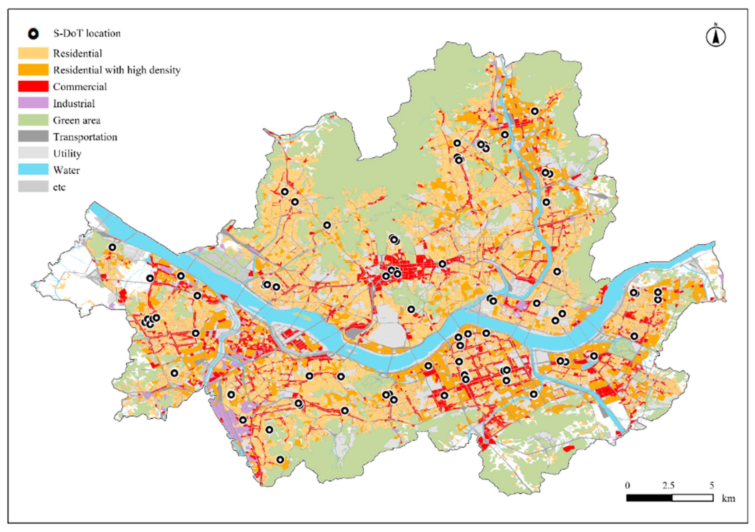
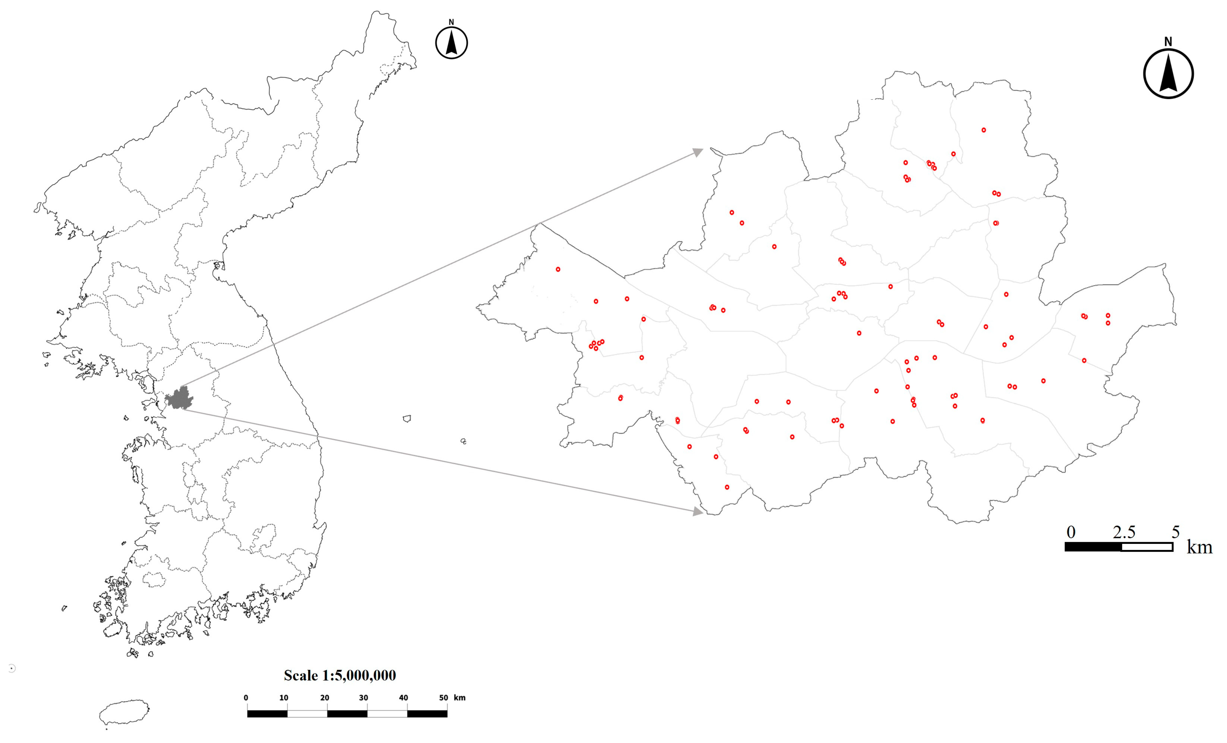
3.2. Study Area and Scope

This study focused on Seoul, Republic of Korea (Figure 2). Seoul is situated in a mid-latitude temperate climate zone at a longitude of 126.97 and a latitude of 37.56, with a population of 10,370,000 and a land area of 605.2 square kilometers. The selected site was based on its high development density and diverse urban configurations. The temporal scope of the study was set to 2022, a year characterized by global heat waves and unusual weather in Seoul. The period was set to one year to observe the impact of all four seasons. The climate of Korea is characterized by distinct seasonal changes. Spring and autumn are typically dry, summer is hot and humid, and winter is cold and dry. As of 2022, according to the Korea Meteorological Administration, the average air temperatures per season were 13.8 °C in spring (March–May), 25.4 °C in summer (June–August), 15.7 °C in autumn (September–November), and −2.03 °C in winter (December–February). The annual average relative humidity is 61.8%, with the lowest at 54.6% in February and March, and the highest at 76.2% in July (Table 1) [56].
The study employed a geographic scale of a 300 m radius around the S-DoT measurement station to capture the urban configuration. Land use which affects air temperature is typically described within a range of 500–1000 m [51,57,58]. Moreover, a physical environment within 500 m is suitable for explaining walking activities [59]. This study specifically chose a 300 m range to concentrate on a small-scale built environment. The S-DoT measurement station provided data for analysis, measuring the air temperature and humidity every hour and the de facto population every 10 min.

3.3. Variables and Data Sources

In this study, the dependent variable was the de facto population, specifically, the average number measured throughout the day. This serves as an indicator of urban vitality. The explanatory variables consisted of the daily average air temperature and urban configuration type (Table 2). We use S-DoT data for air temperature and the de facto population, which were obtained from the Seoul Open Data Plaza [60].
S-DoT was installed as part of Seoul’s smart city policy to discover the data-based administrative foundation and public service citizen experience services [61]. S-DoT gathers urban data through IoT sensors and CCTV to identify urban phenomena such as fine dust, noise, and light pollution in the city. In 2019, 850 S-DoT measurement stations were installed, 250 in 2020, and as of January 2023, a total of 1100 stations were installed [61]. Depending on the purpose of the measurement station, the measurement items vary, and there are 17 types of measurement items, including particulate matter, weather, humidity, lights, noise, vibration, UV rays, wind direction, wind speed, visitors, ozone (O3), odor (NH3, H2S), air pollution (CO, NO2, SO2), and black bulb (city radiant heat measurement) [61] (see Appendix A). Data are measured every 2 minutes for environmental information and every 10 minutes for the de facto populations. As of January 2023, there are a total of 1100 S-DoT stations, but there are 100 stations with sensors that measure both environmental information (air temperature) and de facto population. There are two ways to measure the number of people: counting the MAC addresses of mobile phones in the radius of WiFi AP cells or people counting using CCTV [60]. The S-DoT, which measures the de facto population, has been installed across Seoul to represent different spaces in the city, including tourist destinations such as traditional Hanok villages and Seokchon Lake, commercial areas such as traditional markets, areas around public facilities such as government offices and libraries, and low-, medium- and high-density residential areas (see Appendix B). S-DoT is placed at a height of 2 to 4 m. S-DoT data are managed by the city of Seoul to ensure their accuracy [62].
Urban configuration relates to the scale of the urban canopy, streets, and buildings [19]. We focus on urban configuration, which reflects the scale of buildings, streets, and blocks. So we chose the density variables of building floor area ratio and building coverage ratio, as well as the urban canyon variable measured by the H/W ratio, and the block size variable measured by the density of intersections. Compared to the SVF indicator, the H/W ratio is directly related to analyzing urban configuration because it is measured by the height of buildings and the width of streets and has the advantage of providing specific guidelines for streets and buildings based on the analysis results.
The control variables in the research consisted of land-use characteristics and dummy variables that represented weekdays, weekends, and the four seasons (spring, summer, autumn, and winter). The land-use features included three different ratios, namely commercial, business, and parks. Water areas were present in the 300 m radius surrounding 11 stations; therefore, a dummy variable for water area was used (see Appendix C).

3.4. Methodology

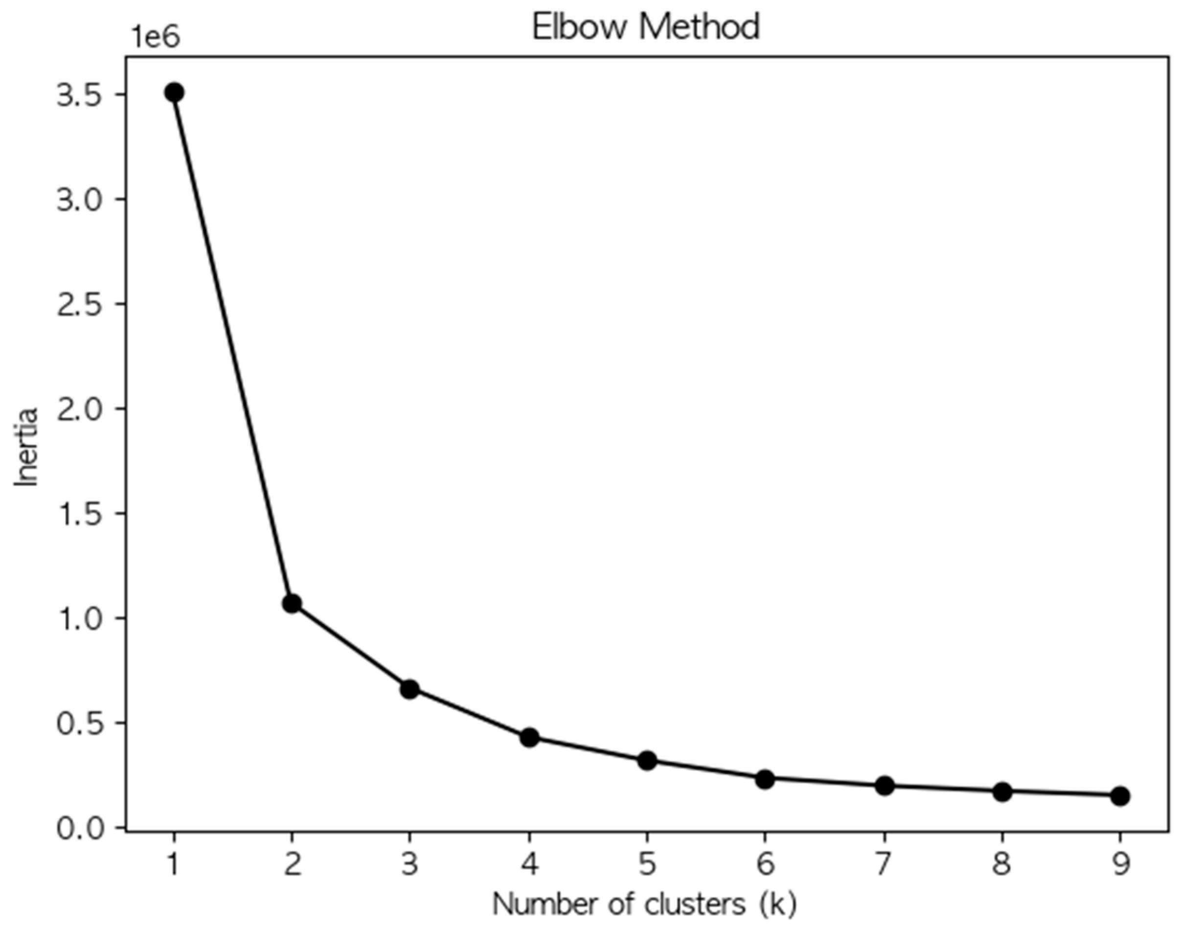
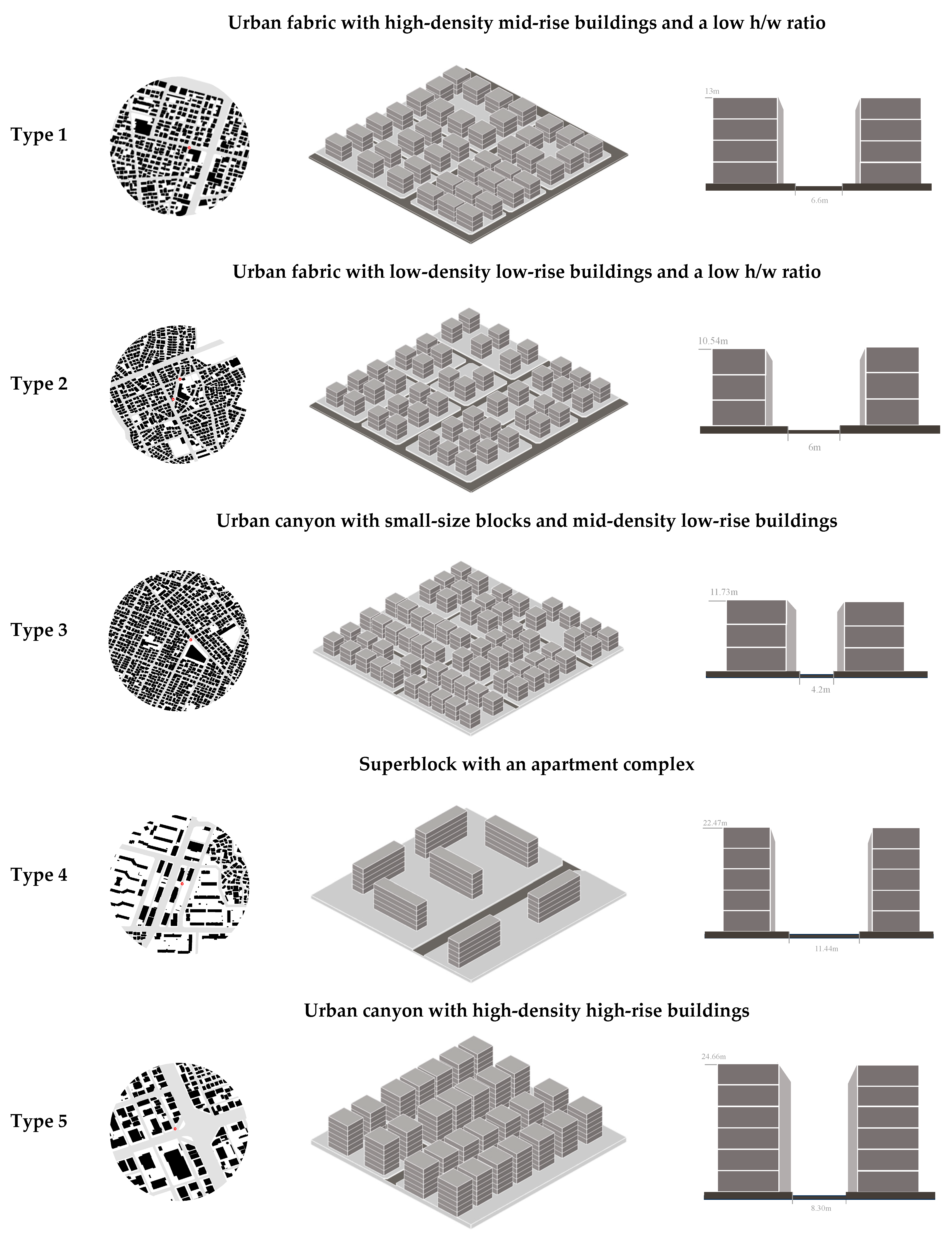
3.4.1. Type of Urban Configuration Using K-Means Clustering

We use four variables to typify urban configuration: density variable of building coverage ratio and building floor area ratio, urban canyon variable measured by H/W ratio, and block size variable measured by intersection density. We aim to derive a representative type of urban configuration in Seoul and understand the relationship between the representative type and air temperature and de facto population. This is to understand which types differ in de facto population considering the air temperature and which types are appropriate to respond to the thermal environment. We used cluster analysis to classify the urban form around the S-DoT measurement stations. The number of clusters is derived through Scree-plot to find the appropriate number of clusters.

3.4.2. Empirical Analysis of the Relationship among Urban Configuration Types, Air Temperature, and De Facto Population Using 2-SLS

Urban configuration and land use directly affect the de facto population, which is a dependent variable, and directly affect air temperature, which is an independent variable. This creates a correlation between the error term and air temperature and causes the endogeneity problem [63]. If the endogeneity problem is not resolved, a bias may occur when estimating the coefficients. To resolve endogeneity, 2-SLS, which conducts regression analysis in two stages, was used.
The empirical analysis involved two models: one for the entire year and another that categorized the year into four seasons (spring, summer, autumn, and winter). The goal was to verify the effect that appeared as a combination of urban configuration variables.
2-SLS utilizes instrumental variables, which must meet two conditions. The first condition for an instrumental variable is that it must have a correlation with an endogenous variable. Second, the instrumental variable must be independent of the error term. In this study; humidity was chosen as the instrumental variable to meet this criterion. Humidity is correlated with air temperature, an endogenous variable, as it tends to be high when air temperatures are high and low when air temperatures are low. However, humidity does not directly impact street vitality, making it a suitable choice as an instrumental variable that satisfies the second condition of independence from the error term.
To assess the appropriateness of the 2-SLS model results, a multiple regression model was constructed and compared to the baseline model. The OLS equation for estimating de facto population is presented as follows (Equation (1)). U T represents the urban configuration type, L U represents land use, and the control variable X represents the weekday/weekend and seasonal dummy variables (spring, summer, autumn, and winter). ϵ is the error term.
D e   f a c t o   P o p u l a t i o n = α 0 + α 1 T e m p + α 2 U T + α 3 L U + α n X n + ϵ
The equation used to estimate the first-stage air temperature in the 2-SLS regression analysis is as follows (Equation (2)). In the first step of 2-SLS, the least-squares method was performed with the instrumental variable humidity ( H U ) and the exogenous variable as independent variables.
T e m p = β 0 + β 1 H U + β 2 U T + β 3 L U + β n Κ n + τ ^
The OLS model was constructed by substituting the estimated T e m p ^ (Equations (3) and (4)) into the de facto population equation in the second step. T e m p ^ is an estimate of Temp and τ ^ means the residual by OLS.
T e m p ^ = β 0 + β 1 H U + β 2 U T + β 3 L U + β n Κ n
T e m p = T e m p ^ + τ ^
The estimation equation (Equation (5)) for substituting the air temperature estimated in the first step into the second-step regression analysis was as follows:
D e   f a c t o   P o p u l a t i o n = γ 0 + γ 1 T e m p ^ + τ ^ + γ 2 U F + γ 3 L U + γ n X n + ϵ

4. Results and Discussion

4.1. Result of Urban Configuration Types

The urban configuration around the measurement stations was categorized using K-means clustering. We established the number of clusters for K-means clustering to be five through a gradual approach based on a Scree Plot (see Appendix D).
Urban configuration types in Seoul were classified according to parameters such as block size, building area ratio, building floor area ratio, and H/W ratio. Depending on their size, blocks were classified into superblocks or small blocks. The building area and floor area ratios were further divided into high, medium, and low density and height categories. The H/W ratio was used to differentiate between urban canyons and areas with low H/W ratios. In summary, this study identified five distinct urban configuration types: mid-rise buildings, low-rise single-family houses, multigenerational houses, Korean apartment complexes, and high-density high-rise buildings.
Type 1 is characterized as an urban fabric with high-density mid-rise buildings and a low H/W ratio. It exhibited the lowest H/W ratio of 2.10, the highest building area ratio of 37.89%, floor area ratio of 131.32%, and intersection density of 317.52 per square kilometer.
Type 2 can be described as an urban fabric with low-density low-rise buildings and a low H/W ratio. The H/W ratio is 1.81, the lowest along with Type 1. The building area ratio was 25.6%, while the floor area ratio was the lowest at 68.67%. The intersection density was 493.84 per square kilometer.
Type 3 is characterized by an urban canyon consisting of small blocks and mid-density low-rise buildings. It had the highest H/W ratio of 2.80, highest building area ratio of 34.44%, floor area ratio of 103.99%, and the highest intersection density of 603.85 per square kilometer.
Type 4 can be described as superblocks with an apartment complex. It had the lowest H/W ratio (2.01), building area ratio (16.01%), floor area ratio (70.26%), and intersection density (139.03) per square kilometer.
Type 5 can be described as an urban canyon with high-density, high-rise buildings. It had the highest H/W ratio (2.96) and building area ratio (37.62%), floor area ratio of 212.89%, and an intersection density of 199.39 per square kilometer. These are the locations and representative case for each of the five types (Figure 3 and Figure 4).
To explore the differences in urban configuration by type, we performed homoscedasticity and Kruskal–Wallis tests (Table 3). Consequently, significant differences were found among the urban configurations by type. To investigate variable differences, we conducted a post hoc analysis using the Kruskal–Wallis test (see Appendix E to Appendix H). In addition, differences were observed in the de facto population (Table 4), and we also performed a post hoc analysis using the Kruskal–Wallis test (see Appendix I). Our analysis of de facto population by type revealed that Type 3 had the highest de facto population, followed by Types 1 and 2, and subsequently by Types 5 and 4.

4.2. Empirical Analysis of the Relationship among Urban Configuration Types, Air Temperature, and De Facto Population Using 2-SLS

We compared the 2-SLS model with the OLS model to determine a more appropriate model and the effect of eliminating endogeneity (Table 5). The OLS model had an adjusted R-squared of 0.182, whereas the 2-SLS model exhibited a significantly higher adjusted R-squared of 0.6948. The Wu–Hausman test was conducted to test the exogeneity of the model and yielded statistical significance at the 1% significance level. The null hypothesis (H0) in the Wu–Hausman test suggests that all endogenous variables are treated as exogenous. This implies the presence of endogeneity in our model. In both models, the effects of the explanatory variables consistently showed the different trend. In the 2-SLS model, the effect of air temperature decreased compared with that in the OLS model, and the effects of urban configuration type, land use, seasonal dummy, and weekday and weekend dummies increased. Removing endogeneity from the 2-SLS model seemed to increase the impact of the underestimated urban configuration type. After comprehensive consideration of the model’s adjusted R-squared and Wu–Hausman test results, the 2-SLS model was deemed more suitable for this study.
In the 2-SLS model, air temperature, urban configuration type, land use, seasonal dummies, and weekday and weekend dummies were statistically significant variables for the de facto population. First, it was observed that as the air temperature increased, the de facto population increased.
Among the five types of urban configuration, Type 2 was designated as the reference group. Type 2 is characterized by urban fabric with low-density low-rise buildings and a low h/w ratio. It is an appropriate type to explain the characteristics and differences of types compared with other urban configuration types. In the 2-SLS model results, Type 1 and Type 3 both had a much larger de facto population than Type 2. In contrast, Type 4 and Type 5 had smaller de facto populations than Type 2.
Type 1 is denser than Type 2 because their building area and floor area ratios were higher. This implies that buildings provided more radiant heat [19]. And type 1 has a higher density of development and is more accessible, resulting in a higher de facto population.
Type 3 exhibited several distinctive characteristics compared with Type 2, including a dense street network and a high density of buildings. Type 3, with dense blocks and deep canyons, has a more increasing de facto population than Type 2. Smaller blocks in urban areas lead to higher permeability and better connectivity between the inside and outside of the block [12,49]. And deep canyons reduce exposure to short-wave radiation during the day [30]. The combination of a high H/W ratio and small blocks appeared to have had a positive impact on the outdoor activities of pedestrians. This is because such urban configurations result in multiple intersections along travel routes, increasing the likelihood of finding shade while walking to destinations.
Type 4, which is characterized by superblocks with apartment complexes, exhibited a lower building area ratio, floor area ratio, and intersection density. As this is an open space, exposure to short-wave radiation affects the air temperature rise [64]. It appears to have a smaller de facto population because pedestrians find it challenging to cope with the climate conditions, such as seeking shade.
Type 5, which is characterized by urban canyons with high density, showed higher building area ratios, building floor area ratios, and H/W ratios than Type 2. High building area and building floor area ratios increase the surface area, producing more heat and accumulating heat over a long period [20].
Types 1 and 5 have the characteristics of a higher building area ratio and floor area ratio than Type 2, but show a contradictory de facto population. The two types differ in terms of building floor area and H/W ratio. Type 1 had a building floor area ratio of 131.32% and H/W value of 2.10, whereas Type 5 had a higher building floor area ratio of 212.89% and H/W value of 2.96, along with a lower de facto population. Increasing building floor area, and H/W ratios results in a shading effect [23,24,25,65], which affects the increase in the de facto population. However, if these ratios exceed a threshold range, the heat radiation from buildings reduces the de facto population [19]. The threshold range at which the de facto population decreases can be regarded as the building floor area ratio and H/W value between Type 1 and Type 5, with the building floor area ratio ranging from 131.32% to 212.89% and the H/W ratio ranging from 2.10 to 2.96.
Concerning the influence of land use characteristics on the de facto population, statistical significance was observed for the proportions of commerce, business, and parks. It was revealed that an increase in the ratio of commerce and business correlated with a rise in the de facto population, which is likely attributable to the concentration of commercial and work activities that promote pedestrian movement. In contrast, an increase in the park ratio was associated with a decrease in the de facto population. This may be because parks are outdoor spaces that directly affect microclimates, and a higher park ratio may deter people from congregating there. Additionally, areas with water area have less available space and less de facto population.
The seasonal dummy has four seasons: spring, summer, autumn, and winter. To examine the differences in the de facto population according to air temperature, the summer with the highest air temperature was set as the reference group. The de facto population was higher in autumn and winter than in summer. In summer, the air temperature is extremely high for outdoor activities; therefore, the de facto population appears to be the lowest. In contrast, during autumn, there appears to be a higher de facto population because of the favorable air temperature conditions for outdoor activities. People’s propensity to avoid outdoor activities during spring due to yellow and fine dust appeared to be a factor in the lower de facto population.

4.3. Seasonal Empirical Analysis of the Relationship among Urban Configuration Types, Air Temperature, and De Facto Population Using 2-SLS

Seasonal analysis was performed to examine the influence of urban configuration on the de facto population (Table 6). The adjusted R-squared was 0.5822 in the spring model, 0.7218 in the summer model, 0.7272 in the autumn model, and 0.4287 in the winter model.
Spring model analysis (Model 3) showed that in urban configuration Types 1 and 3, commercial ratio, business ratio, park ratio, and weekday and weekend dummies were factors that affected the de facto population. Air temperature had no significant effect on the de facto population. Therefore, variations in air temperature appear to have no effect on the de facto population in spring. The data suggest that conditions favorable to outdoor activities are already present with an average air temperature of 7.7 to 19.1 degrees Celsius from March to May [56]. Type 1 is a high-density type, which seems to have contributed to the increase in de facto population. Type 3 is a dense street network with high permeability and road connectivity, which may have contributed to the increase in de facto population. There was no statistically significant variation in the de facto population between Types 4 and 5 compared with Type 2. The air temperature is good for activities in spring, but activity in the park seems to have decreased because people are reluctant to go out owing to fine and yellow dust.
Based on the summer model analysis (Model 4), factors affecting the de facto population were derived, including air temperature, Types 1, 3, 4, and 5, commercial ratio, business ratio, park ratio, and weekday and weekend dummy. Unexpectedly, the de facto population increased in the summer when air temperatures rose. Air temperature increase of 1 degree results in a de facto population increase of 3.70 people. In the summer of 2022, monthly air temperature ranges from 23.3 to 25.7, which is on the lower end of the 21.3 to 35.9 degrees Celsius mentioned in Lin [9] study, where higher air temperatures lead to fewer visitors. It is also within the acceptable air temperature range of 15.2–28.8 degrees Celsius for outdoor activities suggested by Haung et al. [42]. This suggests that the air temperature is within the acceptable range for summer in Seoul, and, therefore, there is a positive correlation between air temperature and de facto population. For the urban configuration type, Types 1 and 3 had higher de facto populations than Type 2. Type 1 had a high density, and Type 3 had small blocks and deep canyons, making it more responsive to air temperature. Types 4 and 5 have low de facto population. Type 4 may have been affected by hotter air temperatures due to direct exposure to shortwave radiation [64], resulting in a lower de facto population. Type 5 is high building density, which increases surface area and accumulates more heat, raising air temperatures and likely reducing de facto population [20]. As the ratio of commerce and business increased, the de facto population increased. The rise in the ratio of business and employment leads to purposeful walking in the same way as in the entire-year model; thus, the de facto population increases. The de facto population appears to decrease in parks with an open space spatial structure, which makes it difficult to cope with an unusual climate. There was no air temperature reduction effect in the water system. The de facto population was higher on weekends than on weekdays. It is hypothesized that numerous recreational activities take place during summer weekends.
The autumn model analysis (Model 5) derived various factors such as air temperature, Types 1, 3, 4, and 5, commercial ratio, business ratio, park ratio, water area dummy, and weekday and weekend dummies, which affected the de facto population. The rise in air temperature by 1 degree led to an increase of 5.27 individuals in the de facto population, which refers to urban vitality. The urban configuration effect in autumn was the same as in summer. Additionally, a higher park ratio contributes to an increase in the current population. Autumn air temperatures promote recreational activities, which have a positive impact on parks. The de facto population was higher on weekends than on weekdays. It appears that numerous leisure walking activities take place on weekends during the autumn.
The winter model analysis (Model 6) identified air temperature, Types 1, 3, 4, and 5, commercial ratio, business ratio, park ratio, and weekday and weekend dummies as factors that affected the de facto population. An increase in air temperature of 1 degree results in a population increase of 28.28 people. Type 5 displays a de facto population that contradicts the summer model (Model 4) and exceeds the de facto population of Type 2. As previously stated, Type 5 possesses an urban structure that increases air temperature. It has the highest building area ratio, building floor area ratio, and H/W ratio, and increases the air temperature owing to the solar radiation emission effect of buildings and the disruption of atmospheric circulation (Je & Jung, 2018) [37].
Comparing summer and winter showed differences in Type 5 and weekday and weekend dummies. During summer, Type 5 had a de facto population that was lower than that of Type 2, whereas it was higher in winter than that of Type 2. Type 5 has a high building density with a high heat capacity, which increases the air temperature. This leads to a decrease in de facto population due to higher air temperatures in the summer but an increase in the winter. In summer, de facto population is higher on weekends than on weekdays, but in winter, it is higher on weekdays. This may be because people are more sensitive to heat in the winter [9], leading to more essential trips than leisure trips.

5. Conclusions

The urban thermal environment is associated with activity in outdoor public spaces [42]. The de facto population is a key measure of urban vitality, and increasing the de facto population has benefits at both individual and societal levels. We conducted an empirical analysis of the types of urban configuration, air temperature, and de facto population using a full-year model and a seasonal model in our research framework. There is an issue of endogeneity that we addressed by using humidity as an instrumental variable and the 2-SLS model. Consequently, variations in de facto population emerge depending on the combination of urban configuration type and air temperature. We have identified urban configuration types that are conducive to urban vitality in Seoul.
The optimum urban configuration type for all seasons is Type 3. Type 3 features an urban canyon with small blocks and mid-density low-rise buildings. It has indicated that a grid structure can be as effective as an urban spatial structure in response to climate change, especially in areas with high H/W ratios, which are advantageous for creating shading effects [23,24,25,65]. This indicates that a combination of these urban configurations can increase the de facto population. Type 4 is the most adverse to de facto population in terms of the thermal environment. Low-rise, low-density buildings and large block sizes are unfavorable to the thermal environment and result in low pedestrian traffic in all seasons.
Urban configuration has conflicting and seasonal effects on the de facto population. Type 5 has a lower de facto population in summer but a larger one in winter than type 2. Urban canyons with high-density high-rise buildings are only favorable in winter. Overall, in order to maintain the de facto population in response to the thermal environment, it is appropriate to avoid large blocks and low-density low-rises and to maintain medium density and low-rises in small blocks, considering the seasons.
This study classified various types of urban configurations and empirically analyzed the correlation between air temperature and the de facto population. Urban configuration interacts with air temperature, affecting both air temperature and the de facto population through radiation, shading, and the influence of the atmospheric circulation system. These findings suggest that considering the air temperature when designing urban configurations is crucial for maintaining the de facto population. Establishing the interrelationship among air temperature, urban configuration, and de facto population is meaningful for formulating urban policies to respond to climate change. These changes can enhance the de facto population by creating an environment with a suitable air temperature.
A notable constraint in classifying urban configuration is the oversight of certain attributes that extend beyond parameters such as density, block size, and the height-to-width (H/W) ratio. In addition, the population density is related to the de facto population but was not included due to multicollinearity issues in the model. Population density is highly correlated with Type 5, dense urban areas, at correlation coefficient of 0.538, and with type 3 at correlation coefficient of 0.540. Instead of population density, the model controls for land uses that generate urban activity, such as commercial, and business floor area ratio.

Author Contributions

Conceptualization, M.P. and H.K.; methodology, M.P. and H.K.; data curation, M.P.; writing—original draft preparation; M.P. and H.K.; writing—review and editing: M.P. and H.K. All authors have read and agreed to the published version of the manuscript.

Funding

This work was supported by the National Research Foundation of Korea (NRF) grant funded by the Korean government (MSIT) (NRF-2018R1C1B6008233).

Data Availability Statement

Data are contained within the article.

Conflicts of Interest

The authors declare no conflict of interest.

Appendix A

Figure A1. S-DoT Sensor (Source: Smart Seoul Portal, https://smart.seoul.go.kr/index.do (accessed on 1 October 2023)).
Land 12 02110 g0a1

Appendix B

Figure A2. S-DoT Location and Land-Use.
Land 12 02110 g0a2

Appendix C

Table A1. Data Sources.
VariablesData Sources
De facto populationSeoul Open Data Square (https://data.seoul.go.kr/ (accessed on 1 October 2023))
Micro
Climate
ATSeoul Open Data Square (https://data.seoul.go.kr/ (accessed on 1 October 2023))
HumiditySeoul Open Data Square (https://data.seoul.go.kr/ (accessed on 1 October 2023))
Urban
Configuration
BCRKorea National Spatial Data Infrastructure Portal (http://www.nsdi.go.kr/ (accessed on 1 October 2023))
FARKorea National Spatial Data Infrastructure Portal (http://www.nsdi.go.kr/ (accessed on 1 October 2023))
ISDNational Transport Information Center (https://www.its.go.kr/ (accessed on 1 October 2023))
H/W RatioKorea National Spatial Data Infrastructure Portal
(http://www.nsdi.go.kr/ (accessed on 1 October 2023))
Land UseCommercial
floor area ratio
Korea National Spatial Data Infrastructure Portal
(http://www.nsdi.go.kr/ (accessed on 1 October 2023))
Business
floor area ratio
Korea National Spatial Data Infrastructure Portal
(http://www.nsdi.go.kr/ (accessed on 1 October 2023))
Park RatioKorea National Spatial Data Infrastructure Portal
(http://www.nsdi.go.kr/ (accessed on 1 October 2023))
Land CoverWater areaKorea National Spatial Data Infrastructure Portal
(http://www.nsdi.go.kr/ (accessed on 1 October 2023))

Appendix D

Figure A3. Scree Plot for K-Means Clustering.
Land 12 02110 g0a3

Appendix E

Table A2. Post hoc Analysis Results of H/W Ratio by Urban Configuration Type.
Type 1Type 2Type 3Type 4
Type 23.06 **
Type 3−6.63 ***−8.14 ***
Type 40.52−0.964.06 **
Type 5−6.99 ***−9.32 ***−0.99−3.30 **
col-row, *** = p-value < 0.001. ** = p-value < 0.05.

Appendix F

Table A3. Post hoc Analysis Results of Building Coverage Ratio by Urban Configuration Type.
Type 1Type 2Type 3Type 4
Type 26.92 ***
Type 32.64 **−4.59 ***
Type 410.56 ***3.23 **8.27 ***
Type 50.14−3.94 **−1.44−6.02 ***
col-row, *** = p-value < 0.001. ** = p-value < 0.05.

Appendix G

Table A4. Post hoc Analysis Results of Building Floor Area Ratio by Urban Configuration Type.
Type 1Type 2Type 3Type 4
Type 28.61 ***
Type 35.01 ***−5.10 ***
Type 47.05 ***−0.144.07 ***
Type 5−7.02 ***−9.74 ***−9.75 ***−8.17 ***
col-row, *** = p-value < 0.001.

Appendix H

Table A5. Post hoc Analysis Results of Intersection Density by Urban Configuration Type.
Type 1Type 2Type 3Type 4
Type 2−5.65 ***
Type 3−10.12 ***−2.89 **
Type 47.30 ***9.79 ***13.52 ***
Type 53.99 **6.59 ***9.45 ***−2.70 **
col-row, *** = p-value < 0.001. ** = p-value < 0.05.

Appendix I

Table A6. Post hoc Analysis Results of De Facto-Population by Urban Configuration Type.
Type 1Type 2Type 3Type 4
Type 2−0.20
Type 3−12.18 ***−10.73 ***
Type 48.21 ***7.73 ***19.32 ***
Type 518.92 ***18.40 ***31.92 ***9.64 ***
col-row, *** = p-value < 0.001.

References

  1. Intergovernmental Panel on Climate Change. The physical science basis. In Contribution of Working Group I to the Fourth Assessment Report of the Intergovernmental Panel on Climate Change; Cambridge University Press: Cambridge, UK; New York, NY, USA, 2007; Volume 996, pp. 113–119. [Google Scholar]
  2. Gehl, J. Life between Buildings; Island Press: Washington, DC, USA, 2011. [Google Scholar]
  3. Lynch, K. Good City Form; MIT Press: Cambridge, MA, USA, 1984. [Google Scholar]
  4. Norton, B.A.; Coutts, A.M.; Livesley, S.J.; Harris, R.J.; Hunter, A.M.; Williams, N.S. Planning for cooler cities: A framework to prioritise green infrastructure to mitigate high temperatures in urban landscapes. Landsc. Urban Plan. 2015, 134, 127–138. [Google Scholar] [CrossRef]
  5. Whyte, W.H. The Social Life of Small Urban Spaces; The Conversation Foundation: Washington, DC, USA, 1980. [Google Scholar]
  6. Park, S.; Kim, S.; Lee, Y.; Kim, J.; Kim, Y. Results of the 2022 Heat-related Illness Surveillance. Public Health Wkly. Rep. 2023, 16, 241–252. [Google Scholar] [CrossRef]
  7. Ballester, J.; Quijal-Zamorano, M.; Méndez Turrubiates, R.F.; Pegenaute, F.; Herrmann, F.R.; Robine, J.M.; Basagaña, X.; Tonne, C.; Antó, J.M.; Achebak, H. Heat-related mortality in Europe during the summer of 2022. Nat. Med. 2023, 29, 1857–1866. [Google Scholar] [CrossRef] [PubMed]
  8. Cho, H.M.; Lee, Y.H. A Study on Heat Wave Adaptation Strategies in Seoul; 2586-484X; The Seoul Institute: Seoul, Republic of Korea, 2018; pp. 1–29. [Google Scholar]
  9. Lin, T.-P. Thermal perception, adaptation and attendance in a public square in hot and humid regions. Build. Environ. 2009, 44, 2017–2026. [Google Scholar] [CrossRef]
  10. Xu, H.; Chen, H.; Zhou, X.; Wu, Y.; Liu, Y. Research on the relationship between urban morphology and air temperature based on mobile measurement: A case study in Wuhan, China. Urban Clim. 2020, 34, 100671. [Google Scholar] [CrossRef]
  11. Perry, J. Climate change adaptation in the world’s best places: A wicked problem in need of immediate attention. Landsc. Urban Plan. 2015, 133, 1–11. [Google Scholar] [CrossRef]
  12. Li, Y.; Schubert, S.; Kropp, J.P.; Rybski, D. On the influence of density and morphology on the Urban Heat Island intensity. Nat. Commun. 2020, 11, 2647. [Google Scholar] [CrossRef]
  13. Azhdari, A.; Soltani, A.; Alidadi, M. Urban morphology and landscape structure effect on land surface temperature: Evidence from Shiraz, a semi-arid city. Sustain. Cities Soc. 2018, 41, 853–864. [Google Scholar] [CrossRef]
  14. Tian, Y.; Zhou, W.; Qian, Y.; Zheng, Z.; Yan, J. The effect of urban 2D and 3D morphology on air temperature in residential neighborhoods. Landsc. Ecol. 2019, 34, 1161–1178. [Google Scholar] [CrossRef]
  15. Zhang, J.; Li, Z.; Hu, D. Effects of urban morphology on thermal comfort at the micro-scale. Sustain. Cities Soc. 2022, 86, 104150. [Google Scholar] [CrossRef]
  16. Hu, Y.; Dai, Z.; Guldmann, J.-M. Modeling the impact of 2D/3D urban indicators on the urban heat island over different seasons: A boosted regression tree approach. J. Environ. Manag. 2020, 266, 110424. [Google Scholar] [CrossRef] [PubMed]
  17. Yang, C.; Kui, T.; Zhou, W.; Fan, J.; Pan, L.; Wu, W.; Liu, M. Impact of refined 2D/3D urban morphology on hourly air temperature across different spatial scales in a snow climate city. Urban Clim. 2023, 47, 101404. [Google Scholar] [CrossRef]
  18. Oke, T.; Cleugh, H. Urban heat storage derived as energy balance residuals. Bound.-Layer Meteorol. 1987, 39, 233–245. [Google Scholar] [CrossRef]
  19. Yang, J.; Yang, Y.; Sun, D.; Jin, C.; Xiao, X. Influence of urban morphological characteristics on thermal environment. Sustain. Cities Soc. 2021, 72, 103045. [Google Scholar] [CrossRef]
  20. Yin, C.; Yuan, M.; Lu, Y.; Huang, Y.; Liu, Y. Effects of urban form on the urban heat island effect based on spatial regression model. Sci. Total Environ. 2018, 634, 696–704. [Google Scholar] [CrossRef] [PubMed]
  21. Sun, F.; Liu, M.; Wang, Y.; Wang, H.; Che, Y. The effects of 3D architectural patterns on the urban surface temperature at a neighborhood scale: Relative contributions and marginal effects. J. Clean. Prod. 2020, 258, 120706. [Google Scholar] [CrossRef]
  22. Hong, S.-W.; Yang, D.; Oh, B.-C. The Impacts of Built Environmental Features on the Land Surface Temperatures for the Heat Wave Seasons in Gwangju, South Korea. J. Korean Sol. Energy Soc. 2019, 39, 67–82. [Google Scholar] [CrossRef]
  23. Bakarman, M.A.; Chang, J.D. The influence of height/width ratio on urban heat island in hot-arid climates. Procedia Eng. 2015, 118, 101–108. [Google Scholar] [CrossRef]
  24. Johansson, E. Influence of urban geometry on outdoor thermal comfort in a hot dry climate: A study in Fez, Morocco. Build. Environ. 2006, 41, 1326–1338. [Google Scholar] [CrossRef]
  25. Zhu, S.; Chen, M.; Lu, S.; Mai, X. Influence of Urban Geometry on Thermal Environment of Urban Street Canyons in Hong Kong. Buildings 2022, 12, 1836. [Google Scholar] [CrossRef]
  26. Chun, B.-S.; Kim, H.-Y. Analysis of urban heat island effect using information from 3-dimensional city model (3DCM). Spat. Inf. Res. 2010, 18, 1–11. [Google Scholar]
  27. Nakata-Osaki, C.M.; Souza, L.C.L.; Rodrigues, D.S. THIS–Tool for Heat Island Simulation: A GIS extension model to calculate urban heat island intensity based on urban geometry. Comput. Environ. Urban Syst. 2018, 67, 157–168. [Google Scholar] [CrossRef]
  28. Joshi, M.Y.; Rodler, A.; Musy, M.; Guernouti, S.; Cools, M.; Teller, J. Identifying urban morphological archetypes for microclimate studies using a clustering approach. Build. Environ. 2022, 224, 109574. [Google Scholar] [CrossRef]
  29. Andreou, E. The effect of urban layout, street geometry and orientation on shading conditions in urban canyons in the Mediterranean. Renew. Energy 2014, 63, 587–596. [Google Scholar] [CrossRef]
  30. Ramírez-Aguilar, E.A.; Souza, L.C.L. Urban form and population density: Influences on Urban Heat Island intensities in Bogotá, Colombia. Urban Clim. 2019, 29, 100497. [Google Scholar] [CrossRef]
  31. Liao, W.; Hong, T.; Heo, Y. The effect of spatial heterogeneity in urban morphology on surface urban heat islands. Energy Build. 2021, 244, 111027. [Google Scholar] [CrossRef]
  32. Sun, R.; Chen, L. Effects of green space dynamics on urban heat islands: Mitigation and diversification. Ecosyst. Serv. 2017, 23, 38–46. [Google Scholar] [CrossRef]
  33. Yang, L.; Qian, F.; Song, D.-X.; Zheng, K.-J. Research on urban heat-island effect. Procedia Eng. 2016, 169, 11–18. [Google Scholar] [CrossRef]
  34. Peng, J.; Jia, J.; Liu, Y.; Li, H.; Wu, J. Seasonal contrast of the dominant factors for spatial distribution of land surface temperature in urban areas. Remote Sens. Environ. 2018, 215, 255–267. [Google Scholar] [CrossRef]
  35. Lee, K.; Hong, W. The study on the heat island and cool island according to trend toward higher temperature in urban: Case study oh Taegu metropolitian city. J. Archit. Inst. Korean 2007, 23, 219–228. [Google Scholar]
  36. Oh, K.-S.; Hong, J.-J. The relationship between urban spatial elements and the urban heat island effect. Urban Des. Inst. Korea 2005, 6, 47–63. [Google Scholar]
  37. Je, M.-H.; Jung, S.-H. Urban heat island intensity analysis by landuse types. J. Korea Contents Assoc. 2018, 18, 1–12. [Google Scholar]
  38. Carmona, M.; Heath, T.; Oc, T.; Tiesdell, S. Urban Spaces-Public Places: The Dimensions of Urban Design. 2003. Available online: https://www.ucl.ac.uk/bartlett/planning/publications/2021/feb/public-places-urban-spaces-dimensions-urban-design-3rd-edition (accessed on 1 October 2023).
  39. Carr, S. Public Space; Cambridge University Press: Cambridge, UK, 1992. [Google Scholar]
  40. Jacobs, J. The Death and Life of Great American Cities; Vintage: New York, NY, USA, 2016. [Google Scholar]
  41. Eliasson, I.; Knez, I.; Westerberg, U.; Thorsson, S.; Lindberg, F. Climate and behaviour in a Nordic city. Landsc. Urban Plan. 2007, 82, 72–84. [Google Scholar] [CrossRef]
  42. Huang, J.; Zhou, C.; Zhuo, Y.; Xu, L.; Jiang, Y. Outdoor thermal environments and activities in open space: An experiment study in humid subtropical climates. Build. Environ. 2016, 103, 238–249. [Google Scholar] [CrossRef]
  43. Montgomery, J. Making a city: Urbanity, vitality and urban design. J. Urban Des. 1998, 3, 93–116. [Google Scholar] [CrossRef]
  44. Xia, C.; Zhang, A.; Yeh, A.G. The varying relationships between multidimensional urban form and urban vitality in Chinese megacities: Insights from a comparative analysis. Ann. Am. Assoc. Geogr. 2022, 112, 141–166. [Google Scholar] [CrossRef]
  45. Cervero, R.; Kockelman, K. Travel demand and the 3Ds: Density, diversity, and design. Transp. Res. Part D Transp. Environ. 1997, 2, 199–219. [Google Scholar] [CrossRef]
  46. Ewing, R.; Cervero, R. Travel and the built environment: A meta-analysis. J. Am. Plan. Assoc. 2010, 76, 265–294. [Google Scholar] [CrossRef]
  47. Long, Y.; Huang, C. Does block size matter? The impact of urban design on economic vitality for Chinese cities. Environ. Plan. B Urban Anal. City Sci. 2019, 46, 406–422. [Google Scholar] [CrossRef]
  48. Kim, S. Urban Vitality, urban form, and land use: Their relations within a geographical boundary for walkers. Sustainability 2020, 12, 10633. [Google Scholar] [CrossRef]
  49. Sung, H.; Lee, S. Residential built environment and walking activity: Empirical evidence of Jane Jacobs’ urban vitality. Transp. Res. Part D Transp. Environ. 2015, 41, 318–329. [Google Scholar] [CrossRef]
  50. Hess, P.M.; Vernez Moudon, A.; Catherine Snyder, M.; Stanilov, K. Site design and pedestrian travel. Transp. Res. Rec. 1999, 1674, 9–19. [Google Scholar] [CrossRef]
  51. Cao, Q.; Luan, Q.; Liu, Y.; Wang, R. The effects of 2D and 3D building morphology on urban environments: A multi-scale analysis in the Beijing metropolitan region. Build. Environ. 2021, 192, 107635. [Google Scholar] [CrossRef]
  52. Lin, J.; Zhuang, Y.; Zhao, Y.; Li, H.; He, X.; Lu, S. Measuring the non-linear relationship between three-dimensional built environment and urban vitality based on a random forest model. Int. J. Environ. Res. Public Health 2022, 20, 734. [Google Scholar] [CrossRef] [PubMed]
  53. Kang, C.-D. Effects of the human and built environment on neighborhood vitality: Evidence from Seoul, Korea, using mobile phone data. J. Urban Plan. Dev. 2020, 146, 05020024. [Google Scholar] [CrossRef]
  54. European Commission. De Facto Population. Available online: https://home-affairs.ec.europa.eu/networks/european-migration-network-emn/emn-asylum-and-migration-glossary/glossary/de-facto-population_en (accessed on 16 November 2023).
  55. Manoli, G.; Fatichi, S.; Schläpfer, M.; Yu, K.; Crowther, T.W.; Meili, N.; Burlando, P.; Katul, G.G.; Bou-Zeid, E. Magnitude of urban heat islands largely explained by climate and population. Nature 2019, 573, 55–60. [Google Scholar] [CrossRef]
  56. Korea Meteorological Administration. Korean Climate Characteristics. Available online: https://www.weather.go.kr/w/obs-climate/climate/statistics/korea-char.do (accessed on 15 October 2023).
  57. Cha, Y.; Kim, H.; Heo, T. The effects of urban land use and land cover characteristics on air temperature in Seoul Metropolitan area. Seoul Stud. 2009, 10, 107–120. [Google Scholar]
  58. Yoon, M.-H.; Ahn, T.-M. An application of satellite image analysis to visualize the effects of urban green areas on temperature. J. Korean Inst. Landsc. Archit. 2009, 37, 46–53. [Google Scholar]
  59. Sung, H.; Lee, S.; Jung, S. Identifying the relationship between the objectively measured built environment and walking activity in the high-density and transit-oriented city, Seoul, Korea. Environ. Plan. B Plan. Des. 2014, 41, 637–660. [Google Scholar] [CrossRef]
  60. Seoul Metropolitan Government. Seoul Open Data Plaza. Available online: https://data.seoul.go.kr/ (accessed on 16 November 2023).
  61. Seoul Metropolitan Government. Smart Seoul Data of Things(S-DoT). Available online: https://news.seoul.go.kr/gov/archives/539344 (accessed on 16 November 2023).
  62. Kim, Y.; Jang, S.; Kim, K.B. Impact of urban microclimate on walking volume by street type and heat-vulnerable age groups: Seoul’s IoT sensor big data. Urban Clim. 2023, 51, 101658. [Google Scholar] [CrossRef]
  63. Gujarati, D. Econometrics by Example; Bloomsbury Publishing: London, UK, 2014. [Google Scholar]
  64. Lee, J.-A.; Jung, D.-Y.; Chon, J.-H.; Lee, S.-M.; Song, Y.-B. An evaluation of human thermal comfort and improvement of thermal environment by spatial structure. J. Korean Inst. Landsc. Archit. 2010, 38, 12–20. [Google Scholar]
  65. Li, X.; Li, Y.; Jia, T.; Zhou, L.; Hijazi, I.H. The six dimensions of built environment on urban vitality: Fusion evidence from multi-source data. Cities 2022, 121, 103482. [Google Scholar] [CrossRef]
Figure 1. Conceptual framework.
Land 12 02110 g001
Figure 2. Study area and locations of S-DoT stations.
Land 12 02110 g002
Figure 3. Location of S-DoT stations by urban configuration type.
Land 12 02110 g003
Figure 4. Representative case and conceptual urban configuration by type.
Land 12 02110 g004
Table 1. Descriptive statistics of air temperature in Seoul for 2022.
SeasonalMonthAir Temperature (°C)Humidity (%rh)
MeanMinMaxMax-MinMeanMin
Winter1−2.2−6.22.68.85521
2−1.1−5.33.89.15521
Spring37.73.212.79.56215
414.81020.610.65517
519.113.92511.15516
Summer623.319.827.57.77318
727.324.2316.87746
825.723.128.95.88039
Autumn922.418.227.296829
1014.610.319.79.46925
11105.615.49.86523
Winter12−2.8−6.61.78.35921
Table 2. Variables and Measurement Methods.
VariablesDescriptionMeasurement
De facto populationAverage de facto population per Day of the S-DoT n = 1 m P o p n m
Micro
Climate
Air
temperature
Average air temperature per Day of the S-DoT (Unit: °C) n = 1 m A T n m
HumidityAverage humidity per Day of the S-DoT (unit: %) n = 1 m H U n m
Urban
Form
Building Coverage
Ratio (BCR)
Average ratio of building area to urbanized area, indicating horizontal building density in the 300 m buffer (unit: %, range: 0~100) k = 1 j B A i k U A i × 100
Floor Area Ratio (FAR)Average ratio of a building gross floor area to urbanized area, indicating vertical building density in the 300 m buffer (unit: %, range: 0~∞) k = 1 j G A i k U A i × 100
Intersection
Density (ISD)
Number of intersections per square kilometer of urbanized area (unit: Count/km2) N O I i U A i
H/W RatioRatio of average building height to average road width within 300 m buffer
(unit: %)
B H i R W i × 100
Land-
Use
Commercial Floor Area
Ratio
Ratio of commercial gross floor area to urbanized area within 300 m of buffer (unit: %, range: 0~∞) k = 1 j C G A i k U A i × 100
Business Floor Area
Ratio
Ratio of business gross floor area to urbanized area within 300 m of buffer (unit: %, range: 0~∞) k = 1 j B G A i k U A i × 100
Park Area RatioRatio of park area within 300 m of buffer (unit: %, range: 0~100) P A i A i × 100
Land coverWater area1 if there is a water surface area,
0 if there is no water surface area
Seasonal
Dummy
SpringMarch, April, May
SummerJune, July, August
AutumnSeptember, October, November
WinterDecember, January, February
Weekend
Dummy
Weekday = 0Monday, Tuesday, Wednesday, Thursday, Friday
Weekend = 1Saturday, Sunday
m : The number of measurements per day; n : Measurement index; P o p n : Population count for each measurement index; A T n : Air Temperature for each measurement index; H U n : Humidity for each measurement index; i : buffer index; k : building index, B A i : Building area of buffer i ; U A i : Urbanized area of buffer i ; G A i k : Building gross floor area of building k of buffer i ; N O I i : The number of intersections of buffer i ; B H i : Average building height of buffer i ; R W i : Average road width of buffer i ; C G A i k : Commercial gross floor area of building k of buffer i ; B G A i k : Business gross floor area of building k of buffer i ; P A i : Park area of buffer i ; A i : Area of buffer i .
Table 3. Descriptive statistics and Kruskal–Wallis test by Urban Configuration Type.
Type 12345Homogeneity of Variance Test
and Nonparametric Test
BCRMean37.8925.6034.4416.0137.62(B.T.) A = 6.2529, p ≤ 0.05/
(K.W.) chi-squared = 39.824, p ≤ 0.001
std3.647.444.788.346.08
FARMean131.3268.67103.9970.26212.89(B.T.) A = 2.5652, p ≤ 0.05/
(K.W.) chi-squared = 51.670, p ≤ 0.001
std17.3327.3517.8432.8344.13
ISDMean317.52493.84603.85139.03199.39(B.T.) A= 4.4220, p = 0.1096/
(K.W.) chi-squared=43.720, p ≤ 0.001
std76.24107.36115.1454.3841.12
H/W RatioMean2.101.812.802.012.96(B.T.) A = 4.3378, p = 0.1143/
(K.W.) chi-squared = 49.076, p ≤ 0.001
std0.320.250.420.800.28
Table 4. Difference of de facto population by urban configuration type.
Type 1Type 2Type 3Type 4Type 5Homogeneity of Variance Test
and Nonparametric Test
De facto
Population
198.84199.57236.00166.53129.65(B.T.) A = 1018.93, p ≤ 0.001/
(K.W.) chi-squared = 766.87, p ≤ 0.001
Table 5. OLS and 2-SLS regression for the effects of urban configuration types on de facto population.
ModelModel 1: OLS ModelModel 2: 2-SLS Model
VariablesβS.E.tβS.E.t
Micro
Climate
Average
Air temperature
4.43 ***0.2219.844.07 ***0.2317.69
Urban Configuration
(ref. Type 2)
Type 1−37.37 ***3.67−10.1827.13 ***4.476.07
Type 3−3.383.67−0.9267.85 ***4.6914.47
Type 4−107.53 ***4.40−24.45−56.87 ***4.82−11.79
Type 5−105.50 ***4.32−24.41−40.70 ***4.87−8.36
Land-
Use
Commercial
Floor area
Ratio
43.65 ***8.065.41172.53 ***9.5118.14
Business
Floor area
Ratio
250.14 ***10.3224.24300.94 ***10.7428.02
Park Ratio−1.93 ***0.15−12.71−1.21 ***0.16−7.67
Land-CoverWater area
(1: yes, 0: no)
−102.88 ***5.28−19.49−43.81 ***5.74−7.63
Seasonal
(ref. Summer)
Spring22.22 ***3.845.7847.01 ***3.1514.93
Autumn47.47 ***3.6413.0571.91 ***2.8525.22
Winter38.37 ***6.735.7058.36 ***5.477.45
Weekend
(1: Weekend, 0: Weekday)
8.37 ***2.323.6018.28 ***2.457.45
Const116.00 ***7.7714.93-
No.16,505
(1) *** = p-value < 0.001, (2) Maximum of VIF = 6.025, (3) for OLS R-square: 0.183, Adj. R-square: 0.182, for 2-SLS R-square: 0.69, Adj. R-square: 0.6898, (4) Wu–Hausman test: 282.7494, p-value < 0.001.
Table 6. 2-SLS Regression results for the effects of urban configuration type on de facto population by season.
Seasonal (2-SLS Model)
ModelModel 3 (Spring)Model 4 (Summer)Model 5 (Autumn)Model 6 (Winter)
VariablesβS.E.tβS.E.tβS.E.tβS.E.t
Micro
Climate
Average
Air temperature
0.672.460.273.70 ***0.477.935.27 ***0.5210.0628.28 ***3.318.55
Urban Configuration
(ref. Type 2)
Type 186.78 **30.392.8655.91 ***9.905.6537.34 ***7.794.7935.28 ***6.365.55
Type 3147.61 ***36.434.0585.87 ***10.418.25113.48 ***7.8514.4637.05 ***6.765.48
Type 4−25.1924.60−1.02−36.35 ***10.81−3.36−48.89 ***8.96−5.45−36.40 ***8.00−4.55
Type 513.5826.550.51−42.52 ***11.73−3.62−24.90 **8.43−2.9527.20 ***7.183.79
Land-
Use
Commercial
Floor area
Ratio
303.01 ***53.205.70215.03 ***22.699.48217.14 ***17.4212.47251.88 ***13.5018.67
Business
Floor area
Ratio
411.24 ***43.889.37342.09 ***22.4215.26354.01 ***19.0218.61220.63 ***21.2210.40
Park Ratio−1.78 ***0.45−3.92−1.54 ***0.31−4.912.60 ***0.406.45−1.81 ***0.29−6.13
Land-CoverWater area
(1: yes, 0: no)
6.4727.990.23−18.0413.12−1.37−38.67 ***9.83−3.93−4.3010.06−0.43
Weekend
(1: Weekend, 0: Weekday)
36.58 ***8.264.4320.39 ***5.293.8520.16 ***4.494.49−19.70 **6.94−2.84
No.3370386151974077
(1) *** = p-value < 0.001. ** = p-value < 0.05, (2) for 2-SLS model 3 R-squared: 0.5834, Adj. R-squared: 0.5822/for 2-SLS model 4 R-squared: 0.7226, Adj. R-squared: 0.7218, for 2-SLS model 5 R-squared: 0.7277, Adj. R-squared: 0.7272/for 2-SLS model 6 R-squared: 0.4301, Adj. R-squared: 0.4287.
Disclaimer/Publisher’s Note: The statements, opinions and data contained in all publications are solely those of the individual author(s) and contributor(s) and not of MDPI and/or the editor(s). MDPI and/or the editor(s) disclaim responsibility for any injury to people or property resulting from any ideas, methods, instructions or products referred to in the content.

