Abstract
In this study, a fuzzy bi-level chance constraint programming (FBCP) model is developed for urban ecological management in Xiamen, China. FBCP has advantages in balancing trade-offs between multiple decision makers and can address fuzzy and stochastic uncertainty in ecosystem management. It also can reflect the impact of different violation risk levels and emission reduction measures on system benefit, ecosystem service value, and land resource allocation. Then, the conversion of land use and its effects at small regional extent (CLUE-S) model is employed to provide the spatial allocation of future land resources under different scenarios. Results reveal that (i) carbon fixation and climate regulation are the major contributors to the ecosystem service value, with a proportion of [15.4, 15.6]% and [18.5, 18.8]%, respectively; (ii) the main environmental problem in Xiamen is the water pollution caused by the excessive discharge of commercial and residential land, with COD and NH3-N account for [68.81, 69.33]% and [67.65, 68.20]% of the total discharge of the city, respectively; (iii) the violation risk p level is the most impact factor, and the schemes with high system benefit would face greater default risk and lower ecological quality; (iv) FBCP model considers the trade-off between economic benefit and ecological quality, while the fuzzy chance constraint programming (FCP) model achieves a high system benefit at the expense of the environment. These findings help decision makers to understand the impact of parameter uncertainty and pollutant discharge policies on system benefit, and adjust land-use patterns to weigh ecological environment protection with urban economic development.
1. Introduction
Ecosystem services refer to the material, culture, and environment that can support and satisfy the survival and life of humankind by maintaining the structure and function of natural ecosystems [1]. Since the mid-20th century, about 770,000 hectares of wetlands in the Sanjiang Plain area of China have been lost due to agricultural expansion and wetland drainage, which has changed the natural landscape pattern. Ecosystem services have declined dramatically, including the loss of wetlands, which has reduced the value of ecosystem services by USD 195 billion over the past 60 years [2]. In addition, since the 21st century, large areas of intertidal wetlands in the coastal areas of the Yangtze River Estuary have been destroyed due to urban development and human activities in China. Breeding ponds and urban buildings have replaced the original natural coastal wetlands, and the local salt marshes and tidal flats continue to decrease. The total ecosystem service value (ESV) of intertidal wetland ecosystems would decrease by about USD 1 billion between 2015 and 2050 [3]. Obviously, the transformation of land-use allocation has a profound impact on the change of ecosystem service value. With the rapid economic growth and the continuous improvement of urbanization level, land use and cover change (LUCC) has become the core issue to study the impact of urban expansion on the ecosystem [4,5]. Therefore, it is necessary to promote effective land planning and management measures to coordinate regional economic development and protect natural ecosystems.
In fact, various uncertainty elements may exist in the process of land resource planning, such as insufficient human practice investigation, the error of subjective judgment, and mutual influences between factors within the system [6,7]. These uncertainties can affect the accuracy of the planning results and even cause wrong decisions to be made [8,9]. Several mathematical optimization methods have been proposed for ecological programming to cope with uncertainty factors such as chance constraint programming (CCP), two-stage stochastic programming (TSP), and fuzzy programming (FP) [10,11,12]. Ou et al. [13] used the CCP model to deal with competitive relationships between land-use types, providing decision makers with a trade-off analysis between optimal economic goals and environmental violation risk. Lv et al. [14] developed a CCP model to address the uncertainty on the right-hand sides of constraints in the urban ecosystem, where ecological environment indicators were regarded as stochastic constraints. Jia et al. [15] employed CCP to provide scientific advice on solving ecosystem problems by adjusting local economic goals and reducing several pollutants at different risk levels of system failure. In general, the CCP method has been widely used, and can effectively deal with the uncertainty parameters expressed by the probability density function [16]. Furthermore, the Monte Carlo simulation (MCS) serves as a probabilistic method for using random numbers to simulate and estimate the stochastic behavior [17]. MCS can overcome the subjective effects on describing random parameters due to insufficient information [18]. Monte Carlo-based chance constraint programming (MC-CCP) is an effective way to solve ecosystem planning problems. In addition, given that the objective function accounting is susceptible to uncertainty in ecological management, Liu et al. [19] used fuzzy programming to calculate the ecosystem service value under different expectations of decision makers, reflecting the impact of the uncertainty of parameters in the objective function on the system benefit. Zaeimi et al. [20] adopted the triangular fuzzy number method to establish the municipal solid waste management model, which effectively eliminated the uncertainty impact caused by the preference of decision makers and minimized the total cost of waste treatment and the total pollutant discharge. Zhang et al. [21] studied the relationship between fuzzy parameters and explored the balance between economic development and ecological protection in Dongying, which provided feasible suggestions for the local economic and ecological development. In the field of ecological management and land-use planning, CCP and FP can effectively deal with the stochastic uncertainties in the constraints of an ecosystem, making a trade-off between the objective function and the environmental violation risk [22].
Although fuzzy chance constraint programming (FCP) can effectively solve the stochastic uncertainty on the constrained right side, the ecosystem is a complex and multi-level system and FCP cannot solve the trade-offs between different decision levels. For example, both upper and lower decision makers have their own goals, and the two are interconnected [23]. The bi-level programming (BP) can balance the goals between the stakeholders from an overall perspective and make comprehensive systematic decisions [24,25]. Jin et al. [26] employed a BP model to evaluate the trade-off between air quality and system costs, which improved air quality and reduced the energy system costs. Ma et al. [27] applied the BP to the water-energy system to solve the conflict between the economic benefit and the electric energy consumption. Su et al. [28] developed a BP model to address energy management and price issues, which combined flexibility in supply and demand to benefit both retailers and customers. Obviously, a bi-level model can help decision makers with a conflict of interest adjust their tolerance to achieve overall satisfaction with the overall system optimization [29]. Unfortunately, no research has yet applied the BP model to ecosystem management. A BP model can also effectively deal with the conflict between environmental protection and economic construction in ecological management.
Although FBCP model can provide quantitative ecological programming results, there are limitations in the spatial allocation of land use. In contrast to the traditional non-spatial allocation of land-use models, conversion of land use and its effects at small regional extent (CLUE-S) is a statistical model based on an analysis of location suitability and combined with dynamic modelling [30,31]. The CLUE-S model consists of the spatial distribution module and the demand module. It can effectively simulate the time change of each land-use type under different scenarios, and predict the future pattern of land-use change. Peng et al. [32] integrated the CLUE-S model and the random forest to predict the spatial dynamics of wetlands in different scenarios, which supported the urban wetland conservation and future sustainable development. Akin et al. [33] combined CLUE-S models with remote sensing information to simulate future changes in crop patterns and assessed the efficiency of future crop pattern modelling, which reduced environmental and agricultural risks. Unfortunately, few studies were reported on coupling CLUE-S with an optimization model for planning urban ecological system.
Therefore, the purpose of this study is to develop a FBCP-CLUE-S model for urban ecological management. The main novelty and the contribution of FBCP-CLUE-S are as follows: (i) FBCP–CLUE-S can effectively address the double fuzzy and stochastic uncertainty in ecological management and check the risk of violation of system constraints; (ii) FBCP–CLUE-S first applies bi-level programming to ecosystem management, and can meet the relatively important decision goals to weigh different decision makers; (iii) FBCP–CLUE-S introduces the optimization results into the spatial analysis to achieve the optimal spatial allocation of land use. Then, FBCP–CLUE-S will be applied to urban ecological management in Xiamen, China. Results can be helpful for analyzing the competition and balance between environmental protection and economic construction and providing satisfactory urban sustainability schemes for all decision makers.
2. Case Study
Xiamen (24°26′ N, 118°04′ E) is located on the southeast coast of Fujian Province, China, covering an area of 1641 square kilometers. It has a sea area of 340 square kilometers and a coastline of 234 km. Xiamen contains six districts (i.e., Siming, Huli, Jimei, Haicang, Tongan, and Xiangan). The population was approximately 5.16 million in 2020, with an average annual population growth rate of 3.87%. Xiamen’s GDP in 2022 was CNY 780.3 billion, an increase of 4.4% over 2021. As a beautiful island city along the southeast coast of China and one of the first five special economic zones to be released in China, Xiamen is known as the “Sea Garden”, forming pillar industries such as tourism, finance, electronics, and machinery. Now, Xiamen takes the lead in putting forward the goal of building a bay-type city with highly developed economic development and a high ecological civilization.
In recent years, Xiamen is relatively short of land, fresh water, and other resources, which makes it difficult to meet the needs of the rapid development of urbanization, population growth, and the transformation of the industrial structure. From 1950 to 2020, the total reclamation area of Xiamen reached 128.7 km2, and 30% of the ecological land was developed into construction land. Large-scale urbanization led to the disappearance of large areas of natural wetlands, and the natural habitat of various biological resources was destroyed and changed. In addition, large amounts of pollutants from urban production and living were discharged into natural ecosystems.
Total emissions of COD, NH3-N, and SO2 were 11,348.69 tons, 845.74 tons, and 1319.78 tons in 2017, respectively, far exceeding the carrying capacity of the local ecosystem. At present, Xiamen is in urgent need of comprehensive treatment of pollutant discharge. This study provides some technical support and decision-making suggestions for local governments. The ecosystem service and eco-environmental parameters required for planning regional ecosystem are shown in Table 1 and Table 2. The parameters of the ecosystem service are derived from practice surveys and the related literature. Ecological environmental parameters (such as pollutant emission thresholds) can be obtained through the Xiamen Ecological Environmental Quality Bulletin (https://sthjj.xm.gov.cn/, accessed on 6 February 2022).

Table 1.
Modeling inputs for ecosystem.
Table 2.
Input parameters related to emission threshold.
3. Methodology
3.1. Fuzzy Bi-Level Chance Constraint Programming (FBCP)
Fuzzy bi-level chance constraint programming (FBCP) is composed of chance constraint programming (CCP), fuzzy programming (FP) and bi-level programming (BP). It can effectively deal with the uncertainty and multi-level problems in the process of ecosystem planning and management.
Chance constraint programming is an optimization method used to handle the stochastic uncertainty of right-hand side constraints, and in turn is used for risk analysis in system analysis planning. The probability of allowing a constraint violation can be expressed as the probability of satisfying the constraint [34,35]. It can be expressed as:
subject to
where Since it is a nonlinear inequality, only in some cases can it be transformed into general linear programming. If the A is determined and the B is random, it can be transformed as:
where , is a cumulative density function and pi is the risk probability of violating constraints [36,37].
When the fuzzy parameter exists only on the objective function, fuzzy programming (FP) can be expressed as [38]:
where “~” represents the fuzzy mathematical symbol, and the represents the fuzzy parameter, where is the center point, and is the spread distance.
According to the fuzzy membership function, the objective function can be converted to:
According to the possibility theory [39,40]:
where Nes(.) represents the necessity level in the event; λ represents the necessity level, which reflects the attitude of the decision makers towards the uncertainty avoidance of the objective function. The necessity level for decision makers is generally above 0.5. Solving the objective of symmetric triangle blur parameter by quantile method, the final objective function can be expressed as follows:
Bi-level programming is an effective method used to mediate conflicts between different interest layers, where the upper level and lower level have an independent goal pursuit [41,42]. It can be defined as:
Since the upper level has a higher priority than the lower level, we first solve the upper level alone, and its result is . Then, solving the lower level, its result is . The decision variable has a maximum tolerance value of r [43]. The membership function of the can be expressed as:
is the most satisfactory result of the upper level. When , decision preference would linearly improve; when , decision preference would linearly reduce. Since the upper level pursues the maximum, deciders would consider that all are satisfied completely, and are dissatisfied completely. Moreover, the optimal solution of the lower level is brought into the upper objective function to obtain the value of . Then, the membership function of target value of the upper level can be expressed as [44]:
The lower level can establish a member function for its own goal to assess satisfaction for each decision outcome. Since the lower level is subject to more restrictions from the upper level, the results of would not appear. The optimal solution of the upper level is brought into the lower objective function to obtain the value of . The lower level would consider that any are dissatisfied completely due to the same reason. Then, the lower level has the membership function for its own target value:
Consequently, the solution of the model transforms into the optimal solution of the overall satisfactory degree. The optimal results of both the upper level and lower level can be obtained [45]:
Subject to:
where η is the overall satisfactory degree. I is a column vector with all elements equal to l and the same dimension as decision variables.
The fuzzy bi-level chance constraint programming (FBCP) can be expressed as follows:
Solve the upper level model first, assuming that is the optimal solution of the upper model, is the optimal solution of the lower model [46], and the membership function of is:
The membership function of the upper level and lower level decision is [47]:
Therefore, the model optimal solution is obtained by solving the overall satisfaction of the upper and lower decisions:
3.2. The Conversion of Land Use and Its Effects at Small Regional Extent (CLUE-S)
The CLUE-S is a model that simulates small-scale land-use changes according to statistical regression methods. Based on data such as land area restrictions, land-use conversion rules, and land-use status map, CLUE-S spatial allocated the land-use requirements according to the size of the total probability of the grid cell [48,49]. The total probability for each grid cell is expressed as:
where TPROPi,j is the total probability of the grid cell i corresponding to land-use type j, Pi,j is the distribution probability of land-use type j on the grid cell i, ELASj is the conversion elasticity of a certain land-use type j, ITERj is an iterative variable of land-use type j.
The land-use type transition would occur in its most likely location, and a logical progressive regression method is applied to calculate the probability of a certain land-use type in each grid [50].
where x1,i, x2,i, …, xn,i are the values of driving factors, β is estimated coefficients of the regression equation.
3.3. Modelling Formulation
Figure 1 presents the framework of the FBCP–CLUE-S model. The upper level, referred as ecological sector, aims to maximize the ecosystem services value to ensure the ecological security of Xiamen. Twelve ecosystem service functions are considered, including carbon fixation, oxygen release, climate regulation, air purification, dust absorption, solid waste purification, water conservation, sewage purification, soil conservation, fertility maintaining, biodiversity, and leisure entertainment. The lower level, referred to as the economic sector, aims to maximize economic benefit, which includes the benefits of construction land and agriculture, and pollutant treatment costs. The ecosystem service value is mainly realized through the evaluation of material quality and value quantity, using the market value method, shadow engineering method, and hypothesis evaluation method. In the model, the ecological land area (PE) and the human activities land area (PI) are the decision variables.
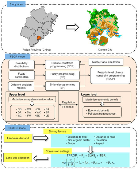
Figure 1.
Framework of the FBCP–CLUE-S model.
Upper level:
Lower level:
The constraints of the FBCP model can be categorized into: (i) the regional available resources; (ii) the allowable discharges of pollutant; (iii) environmental requirement; (iv) policy restraint; and (v) planned land area.
- 1.
- Reallocated land constraints:
- 2.
- Ecological water constraint:
- 3.
- Water resource constraints:
- 4.
- Carbon emission constraint:
- 5.
- Solid waste emission constraint:
- 6.
- COD discharge constraint:
- 7.
- NH3-N discharge constraint:
- 8.
- SO2 discharge constraint:
- 9.
- Sewage discharge constraint:
- 10.
- Percentage of the forestry and grass coverage constraint:
- 11.
- Soil erosion constraint:
- 12.
- Population constraint:
- 13.
- Non-negative constraint:
3.4. Data Acquisition Method
In order to quantitatively investigate the effects of ecological environmental damage on the objective function, two eco-environmental indicators (i.e., soil erosion and forest and grass coverage) were selected, which were more prominent in ecological problems. Annual historical data of ecological and environmental indicators were obtained and expressed as random parameters subject to normal distribution (δ~(μ, σ2)). These random parameters were validated with a Monte Carlo simulation tool. This study selected three different violation probability levels (i.e., 0.05, 0.10, and 0.20), which correspond to high, medium, and low ecological environment requirements. Figure 2 shows the discrete values of these parameters at the different risks of violation. The simulation results are presented in Table 3.
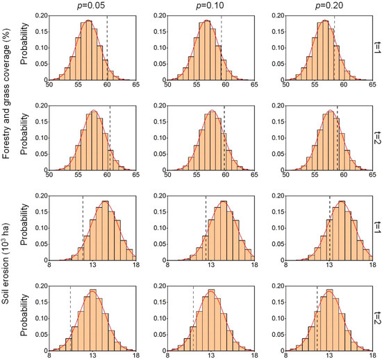
Figure 2.
Probability distributions of forestry and grass coverage and soil erosion.
Table 3.
Results of Monte Carlo simulation.
Xiamen city land-use status map in 2020 is from the National Catalogue Service for Geographic Information (https://www.webmap.cn, accessed on 17 March 2022), with a resolution of 30 m. Digital elevation model (DEM) is derived from the Geospatial Data Cloud (http://www.gscloud.cn, accessed on 17 March 2022), and altitude, slope, aspect, and river data are extracted using Arcgis10.2. In addition, administrative boundaries, roads, and soil data are collected. The land-use types of the initial year are reclassified into six types, including forest, bushland, wetlands, water area, agricultural land, and construction land. The model output cell size is 30 m and the output coordinates are WGS_1984_UTM_Zone_50N. Figure 3 shows spatial differentiation of six driving factors.
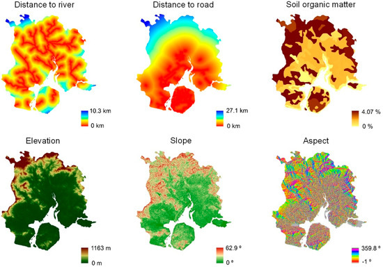
Figure 3.
Spatial differentiation of driving factors.
4. Result Analysis
In this study, three violation possibility levels (p = 0.05, 0.10, 0.20), three pollutant reduction measures (m = 0%, 10%, 20%), and five necessity levels (λ = 0.6, 0.7, 0.8, 0.9, 1.0) were considered, and a total of 45 different scenarios were explored in two planning periods (t = 1, 2). S1, S2, S3 represent the scenarios under λ = 0.6, m = 0%, and p takes 0.05, 0.10, 0.20, respectively; S4, S5, S6 represent the scenarios under λ = 0.6, m = 10%, and p takes 0.05, 0.10, 0.20, respectively; S7, S8, S9 represent the scenarios under λ = 0.6, m = 20%, and p takes 0.05, 0.10, 0.20, respectively. S10, S11, S12 represent the scenarios under λ = 0.7, m = 0%, p takes 0.05, 0.10, 0.20, respectively. By analogy, S43, S44, S45 represent the scenarios under λ = 1.0, m = 20%, p takes 0.05, 0.10, 0.20, respectively.
Figure 4 describes the optimization solution for land-use patterns at different scenarios. In detail, from S1 to S3 (i.e., p increases from 0.05 to 0.20), the ecological land area would decrease from 68.95 × 10³ and 69.91 × 10³ ha to 67.41 × 10³ and 68.57 × 10³ ha, and the human activity land would increase from 92.09 × 10³ and 91.13 × 10³ ha to 93.63 × 10³ and 92.47 × 10³ ha in two periods. This is because the economic benefit of human activity land is far higher than that of ecological land. When the ecological requirements of the model are reduced so that more ecological land is no longer needed to meet the strict constraints, managers tend to develop more efficient construction land at the cost of ecology. However, the higher the p-value is, the higher the system faces a greater risk of ecological and environmental default, and the ecological and environmental risk problems would also be highlighted. Policy makers need to strike a balance between goal pursuit and violation risk. Comparing S3, S6, and S9 (i.e., m increases from 0% to 20%), it can be found that the main manifestation of land change is the conversion of construction land into agricultural land. The planned area for construction land would decrease from 45.79 × 10³ ha and 46.89 × 10³ ha to 45.21 × 10³ ha and 46.46 × 10³ ha, and the planned area of agricultural land would increase from 47.84 × 10³ ha and 45.58 × 10³ ha to 48.16 × 10³ ha and 45.87 × 10³ ha in two periods.
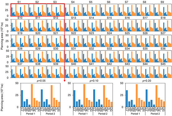
Figure 4.
Planning area under different scenarios [symbols “FT, GL, WL, WA, AL, RC, IL, and OC” denote “forest, bushland, wetlands, water area, agricultural land, commercial and residential land, industrial land, and public land”, respectively].
Furthermore, comparing S1, S10, S19, S28, and S37 (i.e., λ increases from 0.6 to 1.0), λ has little influence on the land planning area, because the decision variables are mainly affected by the constraints, and the necessity level λ mainly affects the maximum value of the decision maker on the expected target. Moreover, the change of pollutant emission threshold has a smaller impact on land planning than the ecological factors, which is because the ecological indicators such as forest and grass coverage rate and soil erosion can directly reflect the local land coverage change and ecological health status. However, the more stringent environmental indicators such as pollutant emission threshold can effectively limit the expansion of urbanization and relieve the ecological pressure caused by excessive pollutants. Ultimately, the contradiction between economic development and environmental quality leads to the competition between human activities and ecosystems for land resources.
Figure 5 presents ESV in different scenarios in two periods. Symbols “CS, RO, CR, PA, DA, SW, WC, SP, SC, FM, BO and LE” denote “carbon fixation, oxygen release, climate regulation, air purification, dust absorption, solid waste purification, water conservation, sewage purification, soil conservation, fertility maintaining, biodiversity and leisure entertainment”, respectively. It can be seen that carbon fixation (CS) and climate regulation (CR) account for the largest proportion of the total ESV, with [15.4, 15.6]% and [18.5, 18.8]%, respectively, which is mainly because the ecosystem can fix large amounts of inorganic and organic carbon. It maintains the humidity of the region, improves the comfort degree of the living environment, and makes great contributions to the carbon cycle and water cycle of the local ecosystem. In addition, solid waste purification (SW) and sewage purification (SP) accounted for about [4.2, 4.5]% and [8.8, 9.1]% of the total ESV, respectively, indicating that the ecosystem plays an important role in pollutant purification and environmental carrying capacity. However, with the increase in p level, all kinds of ecosystem service value would decrease, indicating that the increase in the risk of the system violation level has a great negative impact on the ecological quality. For example, from S4 to S6 (i.e., p increases from 0.05 to 0.20), the oxygen release value would decrease from 6.52 × 10⁹ to 6.37 × 10⁹, and the water conservation value would decrease from CNY 5.13 × 10⁹ CNY 5.02 × 10⁹ in two periods. This is mainly because lower forest and grass coverage and soil erosion indicators would lead to a large amount of forest and bushland destruction, weakening the carbon cycle and water cycle of the ecosystem. It indicates that higher economic benefits are often accompanied by higher violation risk, which means that more ecological environment safety would be sacrificed.
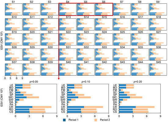
Figure 5.
The ESV of ecosystem under different scenarios.
Figure 6 illustrates the share of the ESV (S1), indicating that the ESV produced by the different land-use patterns would be different. The proportion of forest ecosystem service value is in the dominant position. In S1, the contribution of forest accounted for 55.71% of the carbon fixation value (CS) and 59.89% of the air purification value (PA) in the first period. This is mainly because Xiamen is rich in forest resources, with a high vegetation coverage rate. Forest area accounts for 51.26% of the total ecological land area, which is the main source of energy conversion and gas cycle in the local ecosystem. The wetlands area accounts for 23.94% of the total ecological land area in the first period, while the contribution of wetlands accounts for 33.27% and 29.14% of the solid waste purification value (SW) and sewage purification value (SP). It indicates that wetlands have strong purification ability, and it rely on aquatic vegetation and microorganisms to degrade a large number of organic pollutants, which are the main participants in the treatment of pollutants in the ecosystem. The water area only accounts for 7.40% of the total ecological land area in the first period, but 10.75% of the water conservation value (WC), indicating that the water area can better intercept, permeate and accumulate precipitation, promote water circulation, and play an important role in the regulation of freshwater resources in Xiamen. It can be seen that the land-use pattern would have a profound impact on ESV, but local agricultural products cultivation and mariculture have damaged a large number of forest and coastal wetlands in recent years. Policy makers should strictly control the ecological red line, strengthen natural restoration and ecological restoration, and relieve the ecological pressure brought by economic development.
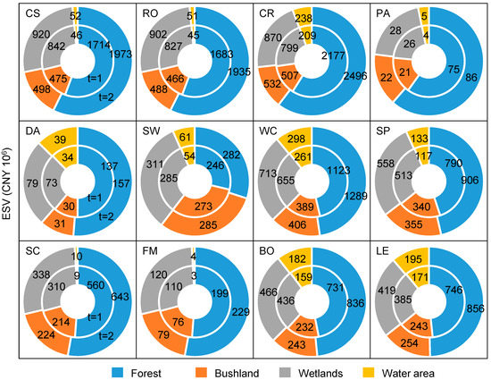
Figure 6.
The share of the ESV of ecosystem (S1).
Table 4 presents the results of coefficients of logistic regression. The magnitude of β value can reflect the extent to which a driving factor influences a certain land type. Results indicate the distribution of forest is mainly affected by soil organic matter and slope, while the distribution of wetlands is mainly affected by soil organic matter and altitude, because their absolute values of β are greater than the other driving factor. When the model is simulated, steep terrain is easier to develop into forest. However, β value of the elevation of wetlands is negative, meaning that the occurrence probability of wetland would be higher in low-lying locations. In addition, the relative operating characteristic (ROC) method is applied to verify the reliability of the simulation results. The closer the value of ROC is to 1, the more accurate the CLUE-S model predicts. The ROC values of all land-use types are higher than 0.7, indicating that the simulation results fit the actual spatial suitable distribution. Figure 7 and Figure 8 present the spatial allocation of land-use optimization in Xiamen from S1 to S9, taking into account the suitability of land use and the impact of human activities. The population of Xiamen city is mostly concentrated in the coastal area, and the northern boundary area is the primeval forest. During the two planning periods, the land-use types in the high-altitude and steep terrain areas would not change significantly, and the ecological land in the central region would expand, while the gently cultivated land in the sea area would gradually develop into construction land.
Table 4.
Values of β from logistic regression.
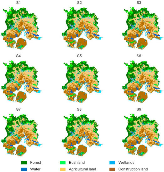
Figure 7.
Spatial allocation of land resources in period 1.
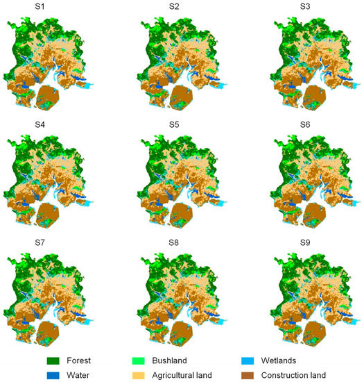
Figure 8.
Spatial allocation of land resources in period 2.
5. Discussion
Figure 9 shows the pollutant discharge situation. In detail, the commercial and residential land is the main source of COD and NH3-N. The annual emission of COD reached [9305, 9454] tons, and the annual emission of NH3-N reached [696, 709] tons in the first period. The COD and NH3-N emitted by commercial and residential land accounted for [68.81, 69.33]% and [67.65, 68.20]% of the whole city. This is because Xiamen is an industrial system dominated by the modern service industry, and the tertiary industry accounts for 60%. The rapid development of the tertiary industry and the continuous expansion of the scale of the urban business circle lead to the discharge of domestic sewage that is higher than the local water environment capacity. Xiamen city is facing a severe water pollution problem now. The rapid development of the tertiary industry and the continuous expansion of the scale of the urban business circle lead to the higher discharge of domestic sewage than the local water environment capacity. Now Xiamen city is facing a serious water pollution problem.
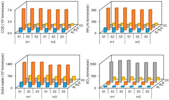
Figure 9.
Pollutant emissions of human activities land. [Symbols “AL, RC, IL, and OC” denote “agricultural land, commercial and residential land, industrial land, and public land”, respectively].
The problem of COD and NH3-N in agricultural land cannot be ignored, accounting for [13.99, 14.27]% and [13.51, 13.79]% of the total emissions, respectively, which mainly comes from the local large-scale chemical fertilizer cultivation mode and breeding industry.
Industrial land is the main source of SO2 emissions, accounting for [72.97, 74.25]% of the total emissions. This may be related to Xiamen’s vigorous expansion of industrial parks in recent years, where product production increases the revenue and also emits a large amount of waste gas to the outside. With the increasing p level, the annual SO2 emissions would increase from 1171 to 1247 tons. Fortunately, pollutant emissions would be reduced during the planning period. This is mainly due to a series of policies formulated by the local government, which improve the efficiency and intensity of the centralized treatment of domestic sewage and the industrial waste gas treatment process and production process. The transformation of industrial structure and the optimization of land distribution would change the severe pollution emission situation.
Figure 10 shows the system benefit and ecosystem service value for 45 different scenarios. From S1 to S3, system benefit would increase from CNY 5.10 × 10¹² (p = 0.05) to CNY 5.27 × 10¹² (p = 0.20), and the ecosystem service value would decrease from CNY 63.78 × 10⁹ (p = 0.05) to CNY 62.83 × 10⁹ (p = 0.20). This is because, as p level increases, a higher system benefit is obtained, but the loss of ecosystem service value would face a higher ecological risk. Decision makers should weigh the system benefit and violation risk in practical planning, and coordinate between economic development and environmental protection. Different emissions reduction measures would also have both economic and ecological impacts. When the emission reduction policy is stricter, the system benefit would decrease slightly, but the ecosystem service value would increase. This can encourage local managers to improve the efficiency of pollutant treatment, and strictly control and reduce pollutant emissions. Further, the results show that different necessity levels (λ) would lead to different system benefit and ecosystem service value. For S1, S10, S19, S28, and S37 (i.e., λ increases from 0.6 to 1.0), the system benefit would gradually decrease from CNY 5.10 × 10¹² to CNY 4.63 × 10¹², and the ecosystem service value would gradually decrease from CNY 63.78 × 10⁹ to CNY 58.08 × 10⁹. It shows that with the increase in necessity level, the system benefit and ecosystem service value would gradually decrease. The higher the necessity level, the less the uncertainty of the objective function and the smaller the system benefit, indicating the conservative attitude of the decision maker towards the expected goal. On the contrary, the lower the necessity level, the more optimistic the decision makers are about the expected goal. Therefore, the uncertainty of the economic data and the preferences of the decision makers have a significant impact on the system benefit. Decision makers need to balance the relationship between expected benefit and risk to seek the optimal decision.
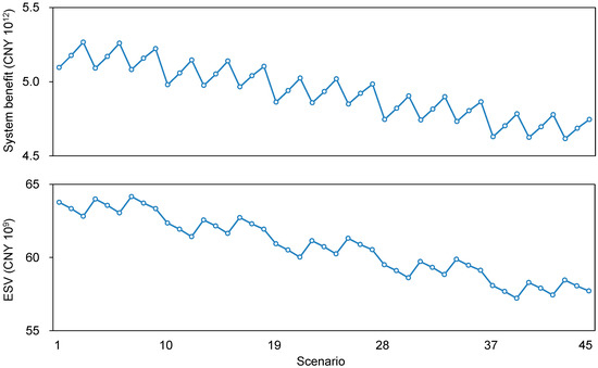
Figure 10.
The system benefit and total ESV under different scenarios.
Figure 11 shows the comparison of results between the FCP and FBCP model. In the first period, the system benefit derived from the FBCP model are more conservative. The FBCP model system benefit would decrease by CNY 0.19 × 10¹² (S1) and CNY 0.27 × 10¹² (S3), but the ecosystem service value would increase by CNY 1.12 × 10⁹ (S1) and CNY 1.49 × 10⁹ (S3). Since the economic benefit of human activity land in the FCP model is far greater than that of ecological land, the decision maker always maximizes the benefit as much as possible under the condition of constraint satisfaction, while ecosystem service value is the intangible asset in the city, and the ecological income should be in the leader–follower relationship in the decision making. This shows that FBCP has more advantages in ecological management, while the growth of the economical FCP model is at the expense of the environment.
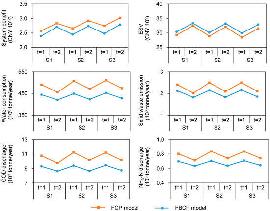
Figure 11.
Comparison of FCP and FBCP model.
Compared with the traditional single model, the FBCP model reduced solid waste emissions by [11.82, 14.25]%, COD emissions by [13.31, 16.06]%, and NH3-N emissions by [13.12, 15.83]%. The FBCP model plays ecosystem service value in the leadership position of the model, which not only improves the ecological carrying capacity of the ecosystem, but also directly reduces the emission of pollution sources. Xiamen is a city with a shortage of fresh water. The FBCP model also showed [9.43, 11.51]% less water consumption than the FCP model, so the FBCP model can also be effectively applied in water resources distribution and effectively save water resources. In general, results show that the FCP model only focuses on system benefit and ignores environment; nevertheless, the FBCP model must ensure ecological quality while pursuing economic maximization. In practice, the optimization results of FCP are not optimal and do not reflect the complexity of the system and reduce the reliability of the system, and the interaction of multiple levels of factors in these problems cannot be solved. The FBCP model considers the trade-offs of economic gain and ecological quality and uses appropriate solutions from an economic and environmental perspective.
6. Conclusions
In this study, a fuzzy bi-level chance constraint programming (FBCP) is first applied to urban ecological management. The spatial allocation of ecological optimization in Xiamen under different scenarios is evaluated by linking the FBCP model to the CLUE-S model in combination with local natural geographical conditions. The developed FBCP method effectively deals with the uncertainty of fuzzy parameters and probability distributions, providing decision schemes at different risk levels. It also coordinates the conflicts of interest between different departments, and deeply analyzes the trade-off between system benefits and ecological quality. Through the solution of FBCP model, the results directly reflect the urban economic benefits, ecosystem service functions, land resource allocation, and other conditions under different risk levels and pollutant emission policies. The land space allocation provided by CLUE-S model is in line with the actual spatial appropriate distribution, which can clearly express the spatial change of the landscape pattern and the impact on the ecological environment under different scenarios.
The developed model shows that: (i) the uncertainty of the economic data and the preferences of the decision makers have a significant impact on the system benefit; (ii) higher p levels bring higher system gains but also greater ecosystem violation risk; (iii) the FCP model pursues economic development maximization at the cost of ecology, but the interests of the two different decision makers in the FBCP model are also effectively balanced; and (iv) the pollutant emission reduction policy only slightly reduces the system benefit but can effectively relieve the environmental pressure. A conservative economic development strategy plays an important role in protecting the ecosystem and the natural environment, but the local economic development would be limited. When regional economic development is given top priority, especially without the management means of ecosystem protection, economic benefit would cause irreversible damage and immeasurable social and economic losses at the expense of the ecosystem. Moreover, the impact of emission reduction policies on the overall benefit of the system is weak, but they play a huge role in promoting the improvement of the ecological environment. To some extent, improving the function and performance of ecosystem service would not only improve the quality of the ecological environment but also promote social and economic development. Accordingly, it is suggested that the relevant authorities should: (i) limit the large-scale urban expansion and strengthen the maintenance of natural vegetation to improve the density of vegetation coverage; (ii) formulate strict emission reduction policies and improve the pollutant removal process; and (iii) accelerate the transformation of low-end manufacturing industries and improve the efficiency of all types of land use.
The application of the FBCP–CLUE-S model has proven to be effective in urban ecological management in Xiamen, where natural ecosystems have been damaged by large-scale reclamation projects and excessive emission of pollution, and the ecological carrying capacity has been degraded. The optimization method presented in this study is generally applicable to the ecological planning and management of other cities in the world. In the actual planning and management process, influenced by complexity and uncertainty factors, the whole range of ecological environment indicators in the model is unrealistic. For different research areas, decision makers can choose different eco-environmental indicators to construct the evaluation ecosystem. In view of the main environmental problems faced by cities, several key indicators with strong representatives are selected to build the evaluation ecosystem. Secondly, the urban natural ecosystem provides various ecological services for human production and life. Using ecosystem services to plan the urban ecological environment is the key to ensuring urban ecological security. Policymakers can choose the appropriate and affordable risks according to actual local development needs. With the help of this pattern, the FBCP–CLUE-S model can provide city managers with scientific advice on urban development schemes.
However, the FBCP–CLUE-S model still has some limitations. There are still complex and non-linear relationships in the actual system. For example, the purification capacity of the ecosystem is greatly affected by the vegetation coverage, terrain, and climate. Water consumption or pollutant discharge are affected by the uncertainty of economic development. In the process of accounting for ecosystem service value, the complexity and uncertainty of the ecosystem also lead to duplication or the omission of errors in the quantification of ecological service function. Further, some important ecological indicators cannot be accurately quantified. The indicators, such as biological abundance, ecological amplitude, and hydrological connectivity, cannot be accurately assessed. Therefore, in future research, more uncertainty factors can be considered, and different ecological environmental indicators can be selected according to the actual conditions of other cities, which can further enhance the FBCP–CLUE-S model and its applicability to urban ecological optimization.
Author Contributions
Conceptualization, L.F. and P.G.; methodology, L.F. and P.G.; software, L.F.; validation, L.F. and S.W.; formal analysis, S.W.; investigation, Z.M.; resources, Z.M.; data curation, Z.M.; writing—original draft preparation, L.F.; writing—review and editing, P.G. and S.W.; visualization, Z.M.; supervision, S.W.; project administration, P.G.; funding acquisition, L.F. All authors have read and agreed to the published version of the manuscript.
Funding
This research was funded by Start-up Project for Advanced Talent of Xiamen University of Technology in the First Half of 2022, grant number YKJ22011R, and The APC was funded by L.F.
Data Availability Statement
Not applicable.
Acknowledgments
The authors would like to extend special thanks to the editor and the reviewers for their constructive comments and suggestions in improving the quality of this paper.
Conflicts of Interest
The authors declare no conflict of interest.
Abbreviations
| f1 | expected ecosystem service value (CNY) |
| f2 | expected economic benefit (CNY) |
| i | ecological land; i = 1, 2, 3, 4 (for forest, bushland, wetlands, water area) |
| j | human activities land; j = 1, 2, 3, 4 (for agricultural land, commercial and residential land, industrial land, public land) |
| t | time periods; t = 1, 2 (for years of 2024–2028, years of 2029–2033) |
| n | element; n = 1, 2, 3 (for N, P, K) |
| PEi,t | planning area of ecological land i (ha) |
| PIj,t | planning area of human activities land j (ha) |
| L | year of the planning period (a) |
| St | total planning area (ha) |
| CACi,t | CO2 absorption amount of ecological land i (t/ha) |
| CT,t | carbon tax (CNY/t) |
| OPt | oxygen price (CNY/t) |
| CREi,t | climate regulation value of ecological land i (CNY/ha) |
| CASi,t | SO2 absorption amount of ecological land i (t/ha) |
| CSRt | SO2 removal cost (CNY/t) |
| ADEi,t | dust absorption amount of ecological land i (t/ha) |
| CDAt | dust removal cost (CNY/t) |
| SWEi,t | solid waste purification amount of ecological land i (t/ha) |
| CWTt | solid waste treatment cost (CNY/t) |
| CCEi,t | water conservation volume of ecological land i (m3/ha) |
| SREi,t | surface runoff coefficient of ecological land i (%) |
| RCt | water price (CNY/m3) |
| CWEi,t | sewage purification amount of ecological land i (t/ha) |
| CSTt | sewage treatment cost (CNY/t) |
| SEEi,t | soil conservation quantity of ecological land i (t/(ha·a)) |
| CESt | soil transportation cost (CNY/t) |
| NCn,t | content of n element in the soil (%) |
| FPn,t | price of fertilizer n (CNY/t) |
| VBEi,t | biodiversity value of ecological land i (CNY/ha) |
| ETVi,t | leisure and entertainment value of ecological land i (CNY/ha) |
| ISVt | ecosystem service value of afforest (CNY) |
| IEBj,t | benefit of human activities land j (CNY/ha) |
| EBEi,t | agricultural products of ecological land i (CNY/ha) |
| WCIj,t | water consumption of human activities land j (ton/ha) |
| AWt | available water resources (t) |
| CPIj,t | COD discharge of human activities land j (t/ha) |
| CPRj,t | COD removal rate of human activities land j (%) |
| CAEi,t | COD purification amount of ecological land i (t/ha) |
| ACDt | COD discharge threshold (t) |
| NPIj,t | NH3-N discharge of human activities land j (t/ha) |
| NPRj,t | NH3-N removal rate of human activities land j (%) |
| NAEi,t | NH3-N purification amount of ecological land i (t/ha) |
| ANDt | NH3-N discharge threshold (t) |
| CEIj,t | carbon emissions of human activities land j (t/ha) |
| ACEt | carbon emissions threshold (t) |
| SWIj,t | solid waste discharge of human activities land j (t/ha) |
| SIRj,t | solid waste recovery rate of human activities land j (%) |
| ASWt | solid waste discharge threshold (t) |
| VAEi,t | vegetation coverage of ecological land i (%) |
| VAIj,t | vegetation coverage of human activities land j (%) |
| PFGt | forestry and grass coverage (%) |
| EREi,t | soil erosion area of ecological land i (ha/ha) |
| ERIj,t | soil erosion area of human activities land j (ha/ha) |
| ASEt | soil erosion threshold (ha) |
| SDIk,t | sewage discharge of human activities land j (t/ha) |
| AWDt | sewage discharge threshold (t) |
| DDIj,t | SO2 emissions of human activities land j (t/ha) |
| DIRj,t | SO2 removal rate of human activities land j (%) |
| ASDt | SO2 discharge threshold (t) |
| MOEi,t | moisturizing coefficient (%) |
| T | conversion coefficient, T = 31.536 × 10⁶ |
| Y | year statistics (a) |
| Qemin | minimum monthly runoff (m3/s) |
| UPj,t | amount of the population of human activities land j (person/ha) |
| TPt | planned total population (person) |
| MINEi,t | minimum area of ecological land i (ha) |
| MINIj,t | minimum area of human activities land j (ha) |
| MAXEi,t | maximum area of ecological land i (ha) |
| MAXIj,t | maximum area of human activities land j (ha) |
References
- Magalhães Filho, L.; Roebeling, P.; Villasante, S.; Bastos, M.I. Ecosystem services values and changes across the Atlantic coastal zone: Considerations and implications. Mar. Policy 2022, 145, 105265. [Google Scholar] [CrossRef]
- Yan, F.Q.; Zhang, S.W. Ecosystem service decline in response to wetland loss in the Sanjiang Plain, Northeast China. Ecol. Eng. 2019, 130, 117–121. [Google Scholar] [CrossRef]
- Li, C.W.; Fang, S.B.; Geng, X.L.; Yuan, Y.; Zheng, X.W.; Zhang, D.; Li, R.X.; Sun, W.; Wang, X.R. Coastal ecosystem service in response to past and future land use and land cover change dynamics in the Yangtze river estuary. J. Clean. Prod. 2023, 385, 135601. [Google Scholar] [CrossRef]
- Fahad, S.; Li, W.; Lashari, A.H.; Islam, A.; Khattak, L.H.; Rasool, U. Evaluation of land use and land cover Spatio-temporal change during rapid Urban sprawl from Lahore, Pakistan. Urban Clim. 2021, 39, 100931. [Google Scholar] [CrossRef]
- Wang, Q.; Wang, H.J. Spatiotemporal dynamics and evolution relationships between land-use/land cover change and landscape pattern in response to rapid urban sprawl process: A case study in Wuhan, China. Ecol. Eng. 2022, 182, 106716. [Google Scholar] [CrossRef]
- Rong, Q.Q.; Zeng, J.N.; Su, M.R.; Yue, W.C.; Cai, Y.P. Prediction and optimization of regional land-use patterns considering nonpoint-source pollution control under conditions of uncertainty. J. Environ. Manag. 2022, 306, 114432. [Google Scholar] [CrossRef]
- Wang, Y.Z.; Guo, X.W.; Yin, H.J.; Zhang, W.G.; Li, Q.K. Spatially distributed footprint families-based simulation–optimization approach for agricultural-ecological resources management under uncertainty. J. Hydrol. 2022, 613, 128319. [Google Scholar] [CrossRef]
- Zhang, H.Y.; Wang, T.T.; Ding, Z.L.; Zhang, X.Q.; Han, L.W. Uncertainty analysis of impact factors of eco-environmental vulnerability based on cloud theory. Ecol. Indic. 2020, 110, 105864. [Google Scholar] [CrossRef]
- Laskookalayeh, S.S.; Najafabadi, M.M.; Shahnazari, A. Investigating the effects of management of irrigation water distribution on farmers’ gross profit under uncertainty: A new positive mathematical programming model. J. Clean. Prod. 2022, 351, 131277. [Google Scholar] [CrossRef]
- Fallahi, F.; Bakir, I.; Yildirim, M.; Ye, Z. A chance-constrained optimization framework for wind farms to manage fleet-level availability in condition based maintenance and operations. Renew. Sustain. Energ. Rev. 2022, 168, 112789. [Google Scholar] [CrossRef]
- Molavi, A.; Shi, J.; Wu, Y.; Lim, G.J. Enabling smart ports through the integration of microgrids: A two-stage stochastic programming approach. Appl. Energy 2020, 258, 114022. [Google Scholar] [CrossRef]
- Xu, Y.; Tan, J.Y.; Wang, X.; Li, W.; He, X.; Hu, X.G.; Fan, Y.R. Synergetic management of water-energy-food nexus system and GHG emissions under multiple uncertainties: An inexact fractional fuzzy chance constraint programming method. Agric. Water Manag. 2022, 262, 107323. [Google Scholar] [CrossRef]
- Ou, G.L.; Tan, S.K.; Zhou, M.; Lu, S.S.; Tao, Y.H.; Zhang, Z.; Zhang, L.; Yan, D.P.; Guan, X.L.; Wu, G. An interval chance-constrained fuzzy modeling approach for supporting land-use planning and eco-environment planning at a watershed level. J. Environ. Manag. 2017, 204, 651–666. [Google Scholar] [CrossRef]
- Lv, J.P.; Li, Y.P.; Sun, J. Monte Carlo simulation based interval chance-constrained programming for regional ecosystem management–A case study of Zhuhai, China. Ecol. Indic. 2018, 85, 214–228. [Google Scholar] [CrossRef]
- Jia, Q.M.; Li, Y.P.; Liu, Y.R. Modeling urban eco-environmental sustainability under uncertainty: Interval double-sided chance-constrained programming with spatial analysis. Ecol. Indic. 2020, 115, 106438. [Google Scholar] [CrossRef]
- Zhang, Q.Q.; Li, Z.; Huang, W. Simulation-based interval chance-constrained quadratic programming model for water quality management: A case study of the central Grand River in Ontario, Canada. Environ. Res. 2021, 192, 110206. [Google Scholar] [CrossRef]
- Baudry, G.; Macharis, C.; Vallée, T. Range-based Multi-Actor Multi-Criteria Analysis: A combined method of Multi-Actor Multi-Criteria Analysis and Monte Carlo simulation to support participatory decision making under uncertainty. Eur. J. Oper. Res. 2018, 264, 257–269. [Google Scholar] [CrossRef]
- Chen, B.; Li, P.; Wu, H.J.; Husain, T.; Khan, F. MCFP: A Monte Carlo Simulation-based Fuzzy Programming Approach for Optimization under Dual Uncertainties of Possibility and Continuous Probability. J. Environ. Inform. 2017, 29, 88–97. [Google Scholar] [CrossRef]
- Liu, H.X.; Li, Y.P.; Yu, L. Urban agglomeration (Guangzhou-Foshan-Zhaoqing) ecosystem management under uncertainty: A factorial fuzzy chance-constrained programming method. Environ. Res. 2019, 173, 97–111. [Google Scholar] [CrossRef]
- Zaeimi, M.B.; Rassafi, A.A. Designing an integrated municipal solid waste management system using a fuzzy chance-constrained programming model considering economic and environmental aspects under uncertainty. Waste Manag. 2021, 125, 268–279. [Google Scholar] [CrossRef]
- Zhang, K.; Li, Y.P.; Huang, G.H.; You, L.; Jin, S.W. Modeling for regional ecosystem sustainable development under uncertainty-A case study of Dongying, China. Sci. Total Environ. 2015, 533, 462–475. [Google Scholar] [CrossRef] [PubMed]
- Yu, L.; Xiao, Y.; Jiang, S.; Li, Y.P.; Fan, Y.R.; Huang, G.H.; Lv, J.; Zuo, Q.T.; Wang, F.Q. A copula-based fuzzy interval-random programming approach for planning water-energy nexus system under uncertainty. Energy 2020, 196, 117063. [Google Scholar] [CrossRef]
- Guo, M.H.; Wang, W.; Chen, R.H.; Li, Y. Research on bi-level model power dispatch considering the uncertainty of source and load. Sustain. Energy Technol. Assess. 2022, 53, 102689. [Google Scholar] [CrossRef]
- Gan, L.; Li, G.Y.; Lin, J.; Zhou, M. A bi-level probabilistic transmission planning with intermittent generations based on life cycle cost. Int. J. Electr. Power Energy Syst. 2017, 90, 306–314. [Google Scholar] [CrossRef]
- Khanchehzarrin, S.; Panah, M.G.; Mahdavi-Amiri, N.; Shiripour, S. A bi-level multi-objective location-routing optimization model for disaster relief operations considering public donations. Socio-Econ. Plan. Sci. 2022, 80, 101165. [Google Scholar] [CrossRef]
- Jin, S.W.; Li, Y.P.; Nie, S. An integrated bi-level optimization model for air quality management of Beijing’s energy system under uncertainty. J. Hazard Mater. 2018, 350, 27–37. [Google Scholar] [CrossRef]
- Ma, Y.; Li, Y.P.; Huang, G.H. A bi-level chance-constrained programming method for quantifying the effectiveness of water-trading to water-food-ecology nexus in Amu Darya River basin of Central Asia. Environ. Res. 2020, 183, 109229. [Google Scholar] [CrossRef]
- Su, S.; Li, Z.N.; Jin, X.L.; Yamashita, K.; Xia, M.; Chen, Q. Bi-level energy management and pricing for community energy retailer incorporating smart buildings based on chance-constrained programming. Int. J. Electr. Power Energy Syst. 2022, 138, 107894. [Google Scholar] [CrossRef]
- Lv, J.; Li, Y.P.; Huang, G.H.; Nie, S.; Gong, J.W.; Ma, Y.; Li, Y. Synergetic management of energy-water nexus system under uncertainty: An interval bi-level joint-probabilistic programming method. J. Clean. Prod. 2021, 292, 125942. [Google Scholar] [CrossRef]
- Kucsicsa, G.; Popovici, E.A.; Bălteanu, D.; Grigorescu, I.; Dumitraşcu, M.; Mitrică, B. Future land use/cover changes in Romania: Regional simulations based on CLUE-S model and CORINE land cover database. Landsc. Ecol. Eng. 2019, 15, 75–90. [Google Scholar] [CrossRef]
- Chasia, S.; Olang, L.O.; Sitoki, L. Modelling of land-use/cover change trajectories in a transboundary catchment of the Sio-Malaba-Malakisi Region in East Africa using the CLUE-s model. Ecol. Modell. 2023, 476, 110256. [Google Scholar] [CrossRef]
- Peng, K.F.; Jiang, W.G.; Deng, Y.; Liu, Y.; Wu, Z.; Chen, Z. Simulating wetland changes under different scenarios based on integrating the random forest and CLUE-S models: A case study of Wuhan Urban Agglomeration. Ecol. Indic. 2020, 117, 106671. [Google Scholar] [CrossRef]
- Akin, A.; Erdoğan, N.; Berberoğlu, S.; Çilek, A.; Erdoğan, A.; Donmez, C.; Şatir, O. Evaluating the efficiency of future crop pattern modelling using the CLUE-S approach in an agricultural plain. Ecol. Inform. 2022, 71, 101806. [Google Scholar] [CrossRef]
- You, L.; Li, Y.P.; Huang, G.H. Modeling regional ecosystem development under uncertainty: A case study for New Binhai District of Tianjin. Ecol. Modell. 2014, 288, 127–142. [Google Scholar] [CrossRef]
- Mianaei, P.K.; Aliahmadi, M.; Faghri, S.; Ensaf, M.; Ghasemi, A.; Abdoos, A.A. Chance-constrained programming for optimal scheduling of combined cooling, heating, and power-based microgrid coupled with flexible technologies. Sustain. Cities Soc. 2022, 77, 103502. [Google Scholar] [CrossRef]
- Wang, Y.M.; Zhu, G.C. Inexact left-hand side two-stage chance-constrained programming for booster optimization in water distribution system. J. Environ. Manag. 2021, 298, 113372. [Google Scholar] [CrossRef]
- Wu, H.; Yue, Q.; Guo, P.; Pan, Q.; Guo, S.S. Sustainable regional water allocation under water-energy nexus: A chance-constrained possibilistic mean-variance multi-objective programming. J. Clean. Prod. 2021, 313, 127934. [Google Scholar] [CrossRef]
- Yu, L.; Li, Y.P. A flexible-possibilistic stochastic programming method for planning municipal-scale energy system through introducing renewable energies and electric vehicles. J. Clean. Prod. 2019, 207, 772–787. [Google Scholar] [CrossRef]
- Inuiguchi, M.; Ramık, J. Possibilistic linear programming: A brief review of fuzzy mathematical programming and a comparison with stochastic programming in portfolio selection problem. Fuzzy Sets Syst. 2000, 111, 3–28. [Google Scholar] [CrossRef]
- Zhang, X.; Huang, G.H.; Nie, X. Robust stochastic fuzzy possibilistic programming for environmental decision making under uncertainty. Sci. Total Environ. 2009, 408, 192–201. [Google Scholar] [CrossRef]
- Van Dijk, D.; Hendrix, E.M.; Haijema, R.; Groeneveld, R.A.; Van Ierland, E.C. On solving a bi-level stochastic dynamic programming model for analyzing fisheries policies: Fishermen behavior and optimal fish quota. Ecol. Modell. 2014, 272, 68–75. [Google Scholar] [CrossRef]
- Beykal, B.; Avraamidou, S.; Pistikopoulos, E.N. Data-driven optimization of mixed-integer bi-level multi-follower integrated planning and scheduling problems under demand uncertainty. Comput. Chem. Eng. 2022, 156, 107551. [Google Scholar] [CrossRef] [PubMed]
- Zhang, Y.F.; Li, Y.P.; Huang, G.H.; Ma, Y.; Zhou, X. Planning a water-food-energy-ecology nexus system toward sustainability: A Copula bi-level fractional programming method. ACS Sustain. Chem. Eng. 2021, 9, 15212–15228. [Google Scholar] [CrossRef]
- Ma, Y.; Li, Y.P.; Huang, G.H.; Liu, Y.R. Water-energy nexus under uncertainty: Development of a hierarchical decision-making model. J. Hydrol. 2020, 591, 125297. [Google Scholar] [CrossRef]
- Gong, J.W.; Li, Y.P.; Lv, J.; Huang, G.H.; Suo, C.; Gao, P.P. Development of an integrated bi-level model for China’s multi-regional energy system planning under uncertainty. Appl. Energy 2022, 308, 118299. [Google Scholar] [CrossRef]
- Lv, Y.; Huang, G.H.; Li, Y.P.; Yang, Z.F.; Liu, Y.; Cheng, G.H. Planning regional water resources system using an interval fuzzy bi-level programming method. J. Environ. Inform. 2010, 16, 43–56. [Google Scholar] [CrossRef]
- Jin, S.W.; Li, Y.P.; Xu, L.P. Development of an integrated model for energy systems planning and carbon dioxide mitigation under uncertainty–Tradeoffs between two-level decision makers. Environ. Res. 2018, 164, 367–378. [Google Scholar] [CrossRef]
- Luo, G.P.; Yin, C.Y.; Chen, X.; Xu, W.; Lu, L. Combining system dynamic model and CLUE-S model to improve land use scenario analyses at regional scale: A case study of Sangong watershed in Xinjiang, China. Ecol. Complex 2010, 7, 198–207. [Google Scholar] [CrossRef]
- Wang, Y.Y.; Chao, B.X.; Dong, P.; Zhang, D.; Yu, W.W.; Hu, W.J.; Ma, Z.Y.; Chen, G.C.; Liu, Z.H.; Chen, B. Simulating spatial change of mangrove habitat under the impact of coastal land use: Coupling MaxEnt and Dyna-CLUE models. Sci. Total Environ. 2021, 788, 147914. [Google Scholar] [CrossRef]
- Jiang, W.G.; Deng, Y.; Tang, Z.H.; Lei, X.; Chen, Z. Modelling the potential impacts of urban ecosystem changes on carbon storage under different scenarios by linking the CLUE-S and the InVEST models. Ecol. Modell. 2017, 345, 30–40. [Google Scholar] [CrossRef]
Disclaimer/Publisher’s Note: The statements, opinions and data contained in all publications are solely those of the individual author(s) and contributor(s) and not of MDPI and/or the editor(s). MDPI and/or the editor(s) disclaim responsibility for any injury to people or property resulting from any ideas, methods, instructions or products referred to in the content. |
© 2023 by the authors. Licensee MDPI, Basel, Switzerland. This article is an open access article distributed under the terms and conditions of the Creative Commons Attribution (CC BY) license (https://creativecommons.org/licenses/by/4.0/).