Abstract
Soil respiration is an important component of the global carbon cycle and is highly responsive to disturbances in the environment. Human impacts on the terrestrial ecosystem lead to changes in the environmental conditions, and following this, changes in soil respiration. Predicting soil respiration and its changes under future climatic and land-use conditions requires a clear understanding of the processes involved. The observation of CO2 fluxes was conducted at an urban grassland, where plants were removed and respiration from bare soil was measured. Nine soil respiration models were applied to describe the temperature dependence of heterotrophic soil respiration. Modified models were suggested, including a linear relationship of the temperature sensitivity and base respiration coefficients with soil temperature at various depths. We demonstrate that modification improves the simulated soil respiration. The exponential and logistic models with linear dependences on the model parameters from the soil temperatures were the best models describing soil respiration fluxes. Variability of the apparent temperature sensitivity coefficient (Q10) was demonstrated, depending on the model used. The Q10 value can be extremely high and does not reflect the actual relationships between soil respiration and temperature. Our findings have important implications for better understanding and accurately assessing the carbon cycling characteristics of terrestrial ecosystems in response to climate change in a temporal perspective.
1. Introduction
Soil respiration represents the second-largest CO2 flux in the terrestrial biosphere and is ten times higher than the current rate of fossil-fuel combustion [1,2,3]. It is an important component of the global carbon cycle and is highly responsive to changes in the local environmental condition [4,5,6,7,8,9,10]: temperature and moisture regime, microbial activity and biomass, freeze–thaw transitions, O2 content, pH, soil carbon and nitrogen, nutrients’ availability, etc. Disturbances of the terrestrial ecosystem lead to changes in the environmental conditions, and following this, disturbances in soil respiration. Understanding the future dynamics of soil systems requires a precise understanding of the responses of soil respiration to changing environmental factors [1,2]. Warming conditions can influence soil respiration by affecting both autotrophic respiration from plant roots and plant-associated symbionts, and heterotrophic respiration due to microbial and animal decomposers [11]. Mathematical models can be used to simulate the impacts of management and potential changes in climate beyond the temporal extent of short-term field experiments.
The temperature dependence of respiration has been mathematically described since the late 19th century [12,13]; however, we still have no mechanistic understanding of how temperature and other environmental factors affect respiration [14]. Various models have been suggested for simulating the short-term responses of soil respiration to variations in air or soil temperature [15,16,17,18,19,20,21,22], and discussions of the accuracy and applicability of temperature sensitivity models continue [11,23,24,25]. Discussions include indirect relationships [9,26,27]. A range of other factors may also strongly influence the apparent response of respiration to temperature, or any deviations, including soil moisture and CO2 diffusivity, the vertical distribution of roots and microbes, and changes in the quality of soil organic matter and its accessibility [25,28,29,30,31,32]. Changes in abiotic and biotic conditions across the soil profile may alter both the actual and apparent (generally reported) temperature response of soil respiration [9,33,34]. Soil temperature changes across the soil profile, and the selection of an appropriate soil depth for inferring temperature sensitivity, may strongly influence the shape of the temperature response curve [2,25,26]. The temperature sensitivity of soil respiration derived from long-term (annual) datasets does not reflect the short-term temperature sensitivity from diurnal data [18,35].
The annual net ecosystem exchange (NEE) for the studied site was described in [36]. The total annual NEE resulted in 163.5 gC/m2. Growing plants accumulate 522.7 gC/m2 in total, but the net annual release of CO2 is higher (686.2 gC/m2) [36]. The studied ecosystem is a source of carbon according to modeling and observation results. In this study, we compared various heuristic models describing the temperature sensitivity of soil respiration. We calibrated soil respiration models against observations of soil efflux from a bare soil site in an urban grassland. We then suggested a procedure for improving model performance considering the variable of the temperature sensitivity coefficient. Finally, we estimated the net gap-filled soil efflux for the vegetation season and analyzed an apparent temperature sensitivity coefficient for various models.
2. Materials and Methods
2.1. Study Site
The observation site (56°28.5′ N, 82°3.2′ E; 170 m a.s.l.) is located on an urban grassland in Tomsk City (West Siberia, Russia). A detailed site description is provided in [36]. The annual average (1981–2010) air temperature is 0.87 °C. Winters are severe and lengthy. The average temperature in January is between −21 °C and −13 °C. The average temperature in July is +18.7 °C. The total annual precipitation is 568 mm, with the maximum in July (75 mm). Snow cover lasts 181 days on average. The total annual sunshine duration is 2123 h [36].
2.2. CO2 Fluxes and Soil Temperature Measurements
The experimental setup for automated soil CO2 flux monitoring operated from 14 April to 20 October 2014 [36]. The LI-8100A (LI-COR Biosciences, Lincoln, NE, USA) flux system with a clear chamber (8100-104C) was used to determine CO2 fluxes [37]. The chamber was closed for 2 min each 20 min. The flux rates were calculated using the LI-8100A software. CO2 flux was estimated based on the exponential growth of CO2 within the chamber [37]. The LI-8100A automatic chamber was placed at the observation site once or twice a month for 2–7 days. In total, 11 experiments with the total duration 33.4 days were carried out.
The bare soil site (trenched soil site) was prepared six months before the experiment. Vegetation at the site was thoroughly cut in September 2013, and large roots were extracted from the surface layer. There was no soil digging to maintain the soil compaction and inner structure, so some fine roots remained in the soil. During summer of 2014, all small sprouts of new vegetation were pulled out from the bare soil site. The ground was kept free of any vegetation during the study period. The CO2 flux measured at the bare soil site in the absence of vegetation represents the heterotrophic respiration flux (HR), which results from a litter and soil organic matter decomposition produced by soil micro-organisms [7].
Air temperature and relative humidity were measured with a thermohydrometer (HMP-45D, Vaisala, Vantaa, Finland). Soil temperature was measured over a 1 h period using a digital temperature probe (APIK-03, IMCES SB RAS, Tomsk, Russia) at the soil surface and 9 different depths of 5, 10, 20, 40, 60, 80, 120, 240, and 320 cm [38].
2.3. Modeling Soil Respiration
Nine models describing the relationships between soil respiration (SR) and temperature were tested (Table 1). The temperature sensitivity coefficient (parameter k) exists in all models, but reflects different types (linear, exponential, power) of increases in respiration with the increasing temperature. The base level of respiration (parameter r) typically represents soil respiration at a certain temperature, excluding model 9, where r indicates the power dependence of respiration to temperature and k corresponds to exponential responses. Models 6–9 have an additional parameter (p) related to a critical temperature level (model 6) or scaling coefficient (models 7–9) for the temperature dependence of soil respiration.

Table 1.
Temperature response functions of soil respiration (SR). k, r, p—model parameters, T1—temperature (°C), Tref = 10 °C, TK = 273.15 °C, T0 = −46.02 °C, Tg = 40 °C, Rg = 8.31 J mol−1 K−1.
The soil respiration models were calibrated according to the in situ-observed carbon dioxide fluxes collected every 20 min. The multiply optimization procedure was conducted using the fminsearch function in MATLAB. The minimum value of the unconstrained multivariable function was identified following the derivative-free method, and the root-mean-square error (RMSE) was used as the minimizing function:
where Oi and Mi are the observed and modeled values, and n is the number of observations.
To determine the performance of the models, the Nash–Sutcliffe coefficient (NSE) [42], RMSE, coefficient of determination (R2), and mean absolute error (MAE) were used:
where and are the mean observed and simulated values, respectively.
We have tested the air, surface, and soil temperatures at nine different depths as variables (T1 in Table 1) governing soil respiration variations, and the temperature variable that yielded the highest model NSE was used in further model modifications.
Each model was modified twice to improve the representations of the observed soil respiration variations during the growing season. The first modification (modification A) considered explicit changes in the temperature sensitivity coefficient with a change in temperature T2:
where k0 is a constant temperature sensitivity coefficient value, and k1 is an increase in the temperature sensitivity with an increase of temperature T2, which represents the air, surface, or soil temperature at nine different depths.
The second model modification (modification B) includes changes in the temperature sensitivity coefficient with temperature T2 (Equation (1)), and changes in the base level of respiration with temperature T3:
where r0 and r1 are the parameters of the linear equation. Gamma model 9B was modified for the second time using a different modification scheme:
Temperatures T2 and T3 in model modification B were selected from all possible combinations of air, surface, and soil temperatures by the maximum NSE coefficient.
The apparent temperature sensitivity coefficient (Q10) was calculated from the results of describing the observed variations in soil respiration with variations in temperature:
where SR(T) and SR(T + 10) are the soil respiration rates at temperatures of T and T + 10, respectively.
3. Results
3.1. Measured Soil Respiration Fluxes
The measured soil fluxes and dates of the experiments are shown in Table 2. The CO2 efflux values were always positive, indicating CO2 emissions to the atmosphere from the soil. Soil CO2 effluxes exhibited clear diurnal patterns. The daytime mean fluxes varied from 0.16 µmol/m2/s in October to 9.9 µmol/m2/s at the beginning of July, while the nighttime fluxes varied from 0.24 µmol/m2/s in October to 10.98 µmol/m2/s in the middle of July (see details in [36]).

Table 2.
Experiments with chamber measurement of soil respiration (µmol m−2 s−1) in 2014. Round-a-day mean (00:00–23:40), day (6:00–21:00), and nighttime (21:20–5:40), and standard deviations.
3.2. Weather Conditions and Soil Temperature
Meteorological conditions during the 2014 growing season were characterized by the air temperature between −12.7 and 36.0 °C. The rapid rise of the temperature with a daily average above 10 °C occurred after 9 June. The average 2014 summer (June–August) temperature was 18.3 °C, which was slightly higher than the long-term average of 16.7 °C. Summer included two locally extreme warm periods with daily T air > 25 °C from 22 to 27 June, and from 6 to 13 July when intense soil warming had begun (Figure 1). The total precipitation in the 2014 growing season (377 mm) was close to the long-term average of 382 mm. In May 2014, it was much wetter (monthly rainfall was 99 mm) in comparison with the long-term average value (41 mm), while in April, June, and September, it was relatively dry, with an anomaly of about 20 mm. The longest dry period without rain lasted from 12 to 25 July.
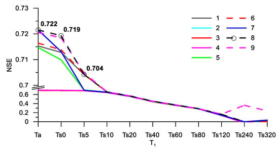
Figure 1.
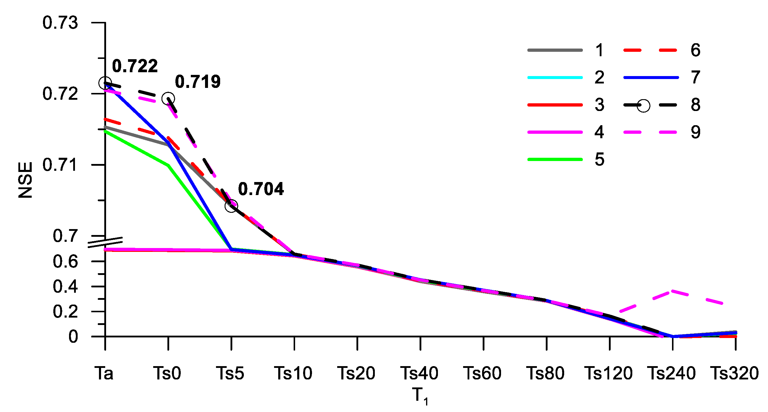
Nash–Sutcliffe efficiency (NSE) coefficient for nine models at various controlling temperatures, T1.
Soil temperatures significantly varied during the year (Table 3). The maximum (+31.2 °C) and the minimum (−1.0 °C) temperatures were observed at the soil surface. Annual soil temperature gradually decreased with the depth. The temperature wave propagated through the soil with a time lag and a decrease of the wave amplitude. The annual amplitude of temperature variations fell to 4.3 °C at a 320 cm depth. Diurnal oscillations of temperature penetrated to a 60 cm depth with the decrease of amplitude from 12.6 to 0.6 °C. The time lag (delay) of the maximum temperature rose to 11 h at 60 cm and to 73.5 days at a 320 cm depth.

Table 3.
Characteristics of soil temperatures for January–December 2014.
3.3. Model Calibration
3.3.1. Basic Models
In this study, model runs were conducted from 1 April to 31 October 2014, with a timestep of 20 min, driven by the observed air, surface, and soil temperatures. For each soil respiration model (see Table 1), the optimal parameters were estimated using data collected from all observation experiments. The parameter optimization experiments for the nine models were conducted several times using different temperatures, as variable T1, governing soil respiration. The air (Ta), surface (Ts0), and soil temperatures at nine different depths (5, 10, 20, 40, 60, 80, 120, 240, and 320 cm) were tested as governing variables. Figure 1 shows the model performance characteristics (NSE coefficient) of models 1–9 with various controlling temperatures. The highest NSE coefficient for each model was obtained using air temperature as a governing variable. The NSE for model 8 (sigmoid) decreased from 0.772 to 0.704 when the governing temperature shifted from air to surface and then to soil temperature at 5 cm. The logistic (model 8, NSE = 0.722), sigmoid (model 7, NSE = 0.722), and Gamma models (model 9, NSE = 0.721) exhibited the best results when describing soil respiration variations with air temperature. The R2 value of the best models was 0.722, yielding a correlation coefficient between the modeled data and observations of 0.849, and a residual standard error (RMSE) of 0.985. Of the nine models, the Q10 (model 2) and exponential (model 3) models had lower NSE (0.692) and higher RMSE (1.038) values. These results indicate that the increasing air temperature positively contributed to soil respiration, but the temperature sensitivity changed with changes in temperature. The optimal model parameters and model goodness characteristics are provided in Table 4. According to the MAE between the best and worst models, changing the model equation for the soil respiration simulation decreased the model error by 0.057 µmol/m2/s, or 7.2%. The air temperature was the best variable controlling soil respiration for any model used. The following model modifications used air temperature, as variable T1.

Table 4.
The optimal model parameters (r, k, p) and model goodness characteristics (NSE, R, MAE). MAE is in µmol m−2 s−1. The best performance metrics indicated in bold.
3.3.2. Model Modification A
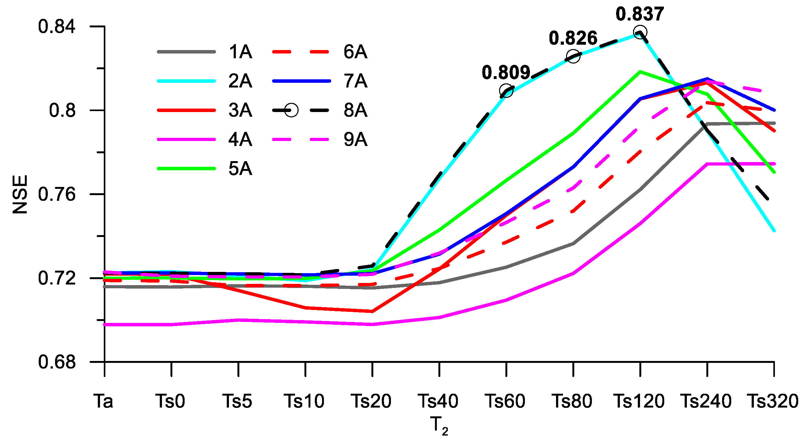
The first modification of the models (modification A) considers an explicit change in the temperature sensitivity coefficient, k, with a change in temperature T2 (Equation (1)). The variable controlling the temperature sensitivity coefficient was selected from the set of air, surface, and soil temperatures. Figure 2 shows the model suitability (NSE coefficient) for various temperature parameters, T2, controlling the changes in model parameter k. The model optimization results are provided in Table 4. The governing temperature resulting in the best model performance was always the deep-layer soil temperature.
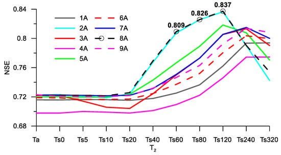
Figure 2.
Nash–Sutcliffe efficiency (NSE) coefficient for nine models with modification A at various controlling temperatures, T2.
Depending on the selected model, the temperature controlling the temperature sensitivity coefficient was the soil temperature at depths of 120 cm (models 2A, 5A, 8A), 240 cm (models 3A, 6A, 7A, 9A), or 320 cm (models 1A and 4A). The Q10 (model 2A) and sigmoid (model 8A) models exhibited the best results (Figure 2) when simulating the soil respiration temperature dependencies. The NSE (0.837) and R2 (0.915) values for these models were considerably higher than for the other six models, where NSE varied in the range of 0.775 to 0.815. The RMSE (0.753) value of the sigmoid model (8A) was 14.9% lower than that of the Arrhenius model (4A). The Arrhenius model with modification A exhibited the worst results, but the efficiency of model 4A (NSE = 0.775) was higher than that of any model that had not undergone modification A. The application of the linear dependence of temperature sensitivity to soil temperature (Equation (1)) improved the soil respiration prediction performance of any model used. The parameters (k, r, p) of the modified models differed from those of the basic models (Table 4). The relative changes in parameter k (ratio of k for the base model to k0 for model modification A) varied from 0.6 (model 7A) to 1.79 (model 3A). The relative influence of the soil temperature on the temperature sensitivity in most models (ratio of k1 × Ts to k0, where Ts is the mean soil temperature for the modeling period) was negative, excluding the Arrhenius and Gamma models (4A and 9A). This shows that the temperature sensitivity of soil respiration decreased with the increasing temperature. Parameters r and p were also changed to maintain the efficiency of the models.
3.3.3. Model Modification B
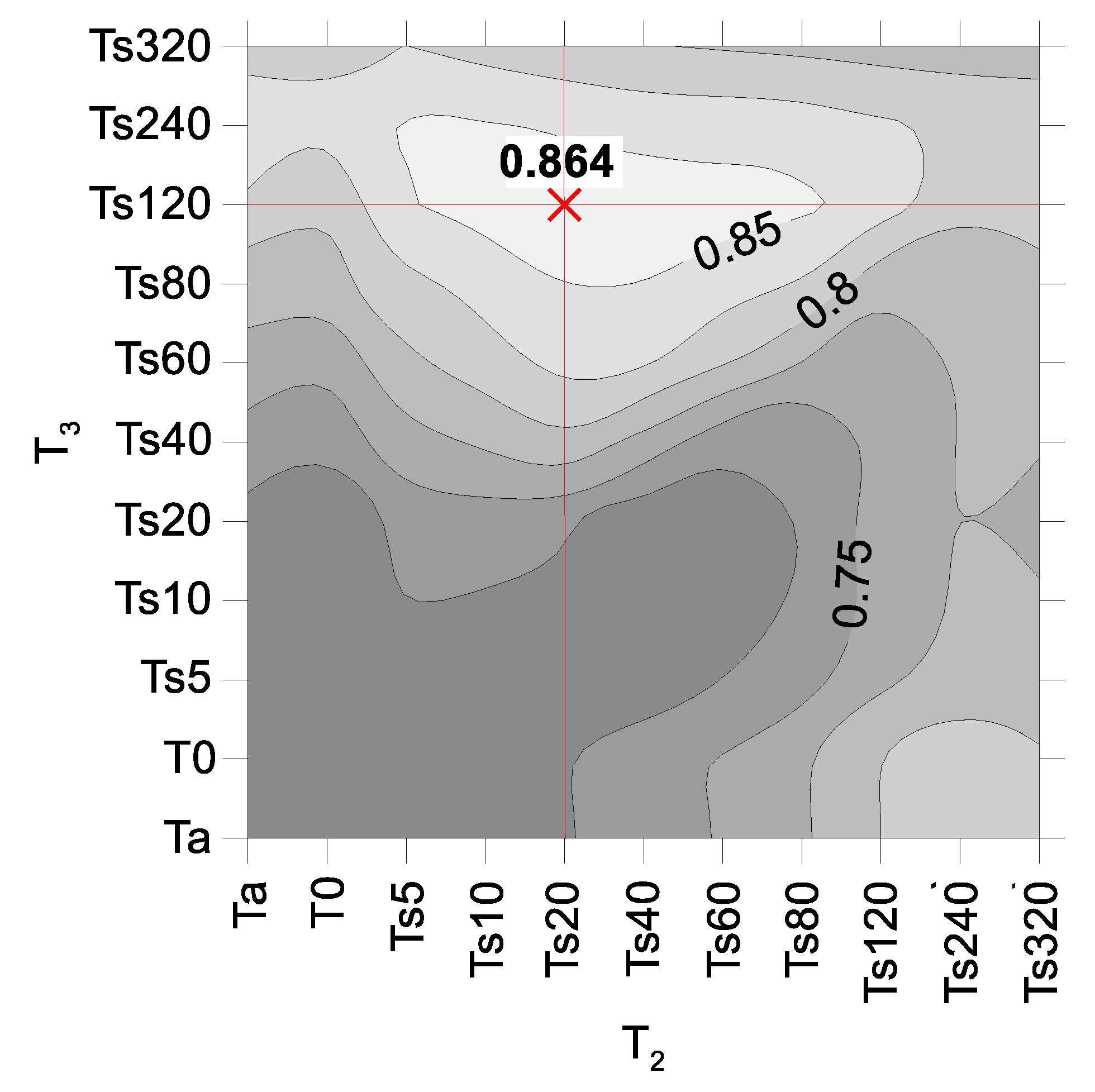
The second modification of the models (modification B) included changes in the temperature sensitivity coefficient with changes in temperature T2 (Equation (1)), and changes in the base level of respiration with changes in temperature T3 (Equation (2)). Air temperature was used as parameter T1, which governed the short-term responses of soil respiration. Parameters T2 and T3 were selected from all combinations of air, surface, and soil temperatures. The model parameters were optimized for each pair of T2 and T3, and the pair of governing temperatures with the highest NSE was used in the resulting model. A map of the distribution of NSE for model 3B in the coordinates of temperatures T2 and T3 is shown in Figure 3. The local maximum NSE (0.864) for model modification 3B corresponded to the soil temperature at 20 cm (Ts20), as variable T2, and the soil temperature at 120 cm (Ts120) as variable T3. The optimal model parameters are provided in Table 4. The logistic model (7B) using the soil temperatures at 20 and 120 cm as variables for the modification of the basic model parameters exhibited the highest NSE (0.866) and R (0.931) values. The exponential model (3B) also agreed well with the observed data. The RMSE values for models 7B and 3B were 0.683 and 0.687. The accuracy of all investigated models with modification B was reasonable. Even the worst model (linear model 1B) exhibited higher NSE (0.821) and R (0.906) values than most of the models with modification A (NSE ranging from 0.775 to 0.837) and any base model without modifications (NSE ranging from 0.692 to 0.722).
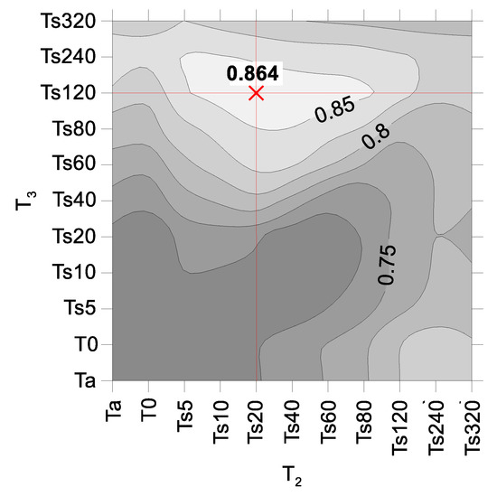
Figure 3.
NSE coefficient for model 3B at various combinations of governing temperatures T2 and T3.
3.4. Modeled Soil Respiration Fluxes
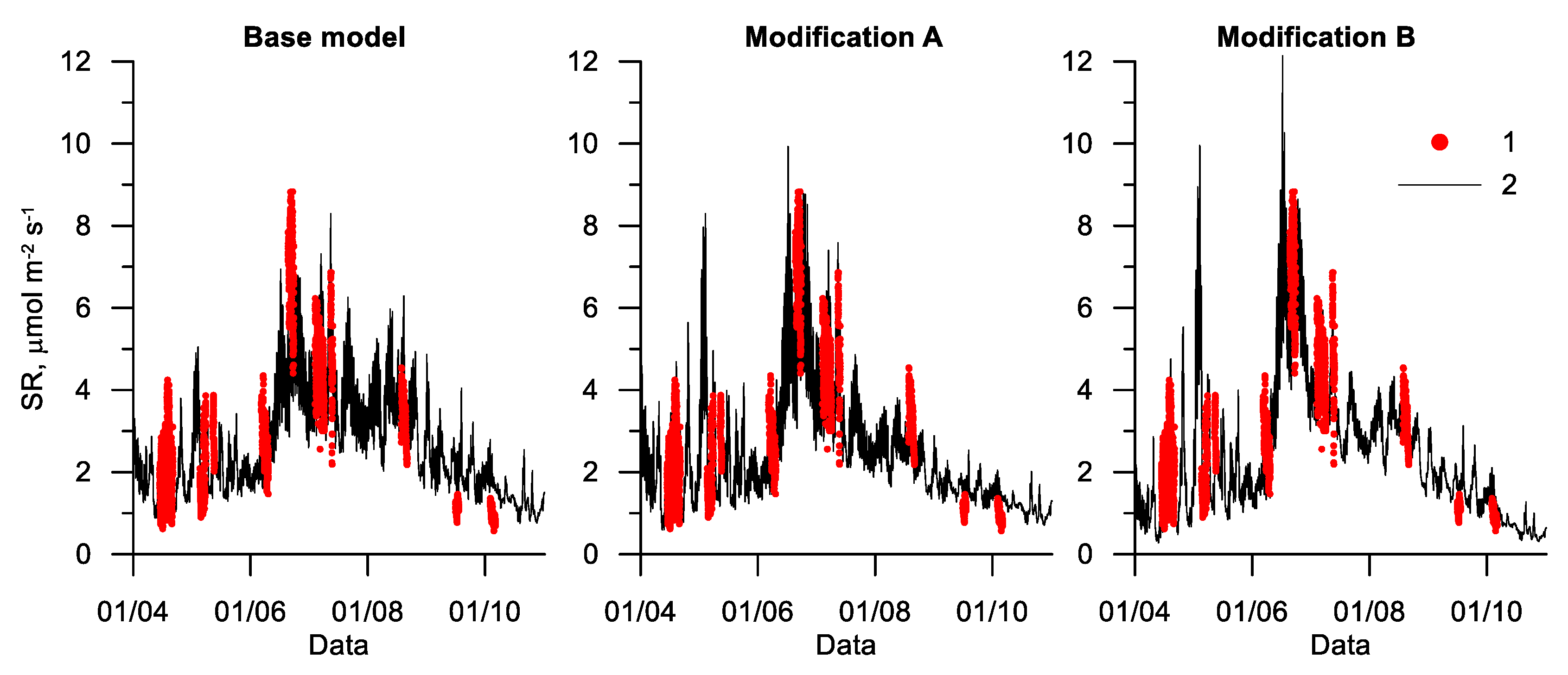
The overall seasonal patterns in soil respiration followed the seasonal changes in air temperature (Figure 4). At the beginning of the growing season, the respiration effluxes were small. However, the soil respiration in all studied models exhibited relatively large daily variations during April and May 2014. After 15 June, when the daily air temperature increased to 15 °C, the modeled fluxes exceeded 4.0 µmol/m2/s in base exponential model 3. The modeled efflux then decreased from August or September (Figure 4). The minimum soil respiration rates were observed at the end of October, when the night air temperature became negative.
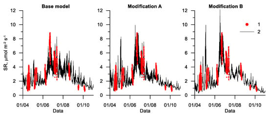
Figure 4.
Seasonal course of observed (1) and modeled (2) soil respiration fluxes, 20-min data. Exponential model (model 3) with modifications A and B.
The shape of the seasonal course and magnitude of the diurnal variations in soil respiration varied between the base models and their modifications (Figure 4). The base models (Table 1) exhibited lower variations in the CO2 effluxes during the study period. Although the main factor controlling soil respiration was air temperature, the amplitude of the diurnal variations in model modifications A and B was controlled by the deep-layer soil temperature. The changes in the temperature sensitivity coefficient according to model modification A (Equation (1)), and subsequent changes in the base level of respiration due to model calibration, resulted in an increase in the diurnal variations of soil respiration in the middle of summer. The soil respiration values determined by model modification B (Equations (1) and (2)) were higher in May and June than those determined by the base model, but the frequency of the variations was lower.
The observation data cover only about 15% of the total growing season. Therefore, gap-filling procedures need to be established for providing a complete dataset and estimations of the net respiration flux. All nine models and their modifications were applied to construct a continuous time series of soil respiration data and calculate the average growing season soil respiration. A significant difference in the average soil respiration rates was detected between the base models and modifications A and B. The statistical analysis results of the modeled soil respiration fluxes are shown in Table 5. The simulated average CO2 effluxes ranged from 2.54 to 2.65 µmol/m2/s for the base model, from 2.36 to 2.60 µmol/m2/s for model modification A, and from 2.30 to 2.58 µmol/m2/s for model modification B.

Table 5.
Statistical characteristics of simulated CO2 soil efflux for April–October. All values are in µmol m−2 s−1.
The estimated soil effluxes decreased as the complexity of all models increased (applying the model modifications). However, the range of the variations in the average soil respiration between the models increased. The median soil efflux value (Table 5) was lower than the mean values, and this disparity increased after the model modifications. The standard deviation (STD) of the estimated soil respiration values (Table 5) for model modification B was higher than that for model modification A. The STD values of base models 1–2 were lower than those of the modified models. The highest CO2 effluxes, which exceeded 12.0 µmol/m2/s, were obtained using models 2A, 8A, and 8B, while the highest effluxes determined by base models 7, 8, and 9 were only 6.40 µmol/m2/s. The lowest values ranged from 0.04 µmol/m2/s for model 5A to 0.75 µmol/m2/s for models 2 and 3. Zero and negative minimal values were obtained for power models (6, 6A, and 6B) and linear models (1, 1A, and 1B). Meaningless negative and zero values of soil respiration are the result of applying the formal model approach for a complex biological process, as a generation and emission of carbon dioxide from the soil. Negative soil CO2 efflux was obtained at air temperatures below −4.1 °C for model 1, and zero efflux for model 6 corresponded to air temperatures below −7.0 °C, while observed air temperatures for models’ calibration were in the range from −3.3 to +36.0 °C. Therefore, linear and power models (models 1 and 6) are not suitable for application outside the temperature range, where modeling results are not verified by the direct measurements. All other models yielded physically reasonable estimations for high-variable CO2 effluxes.
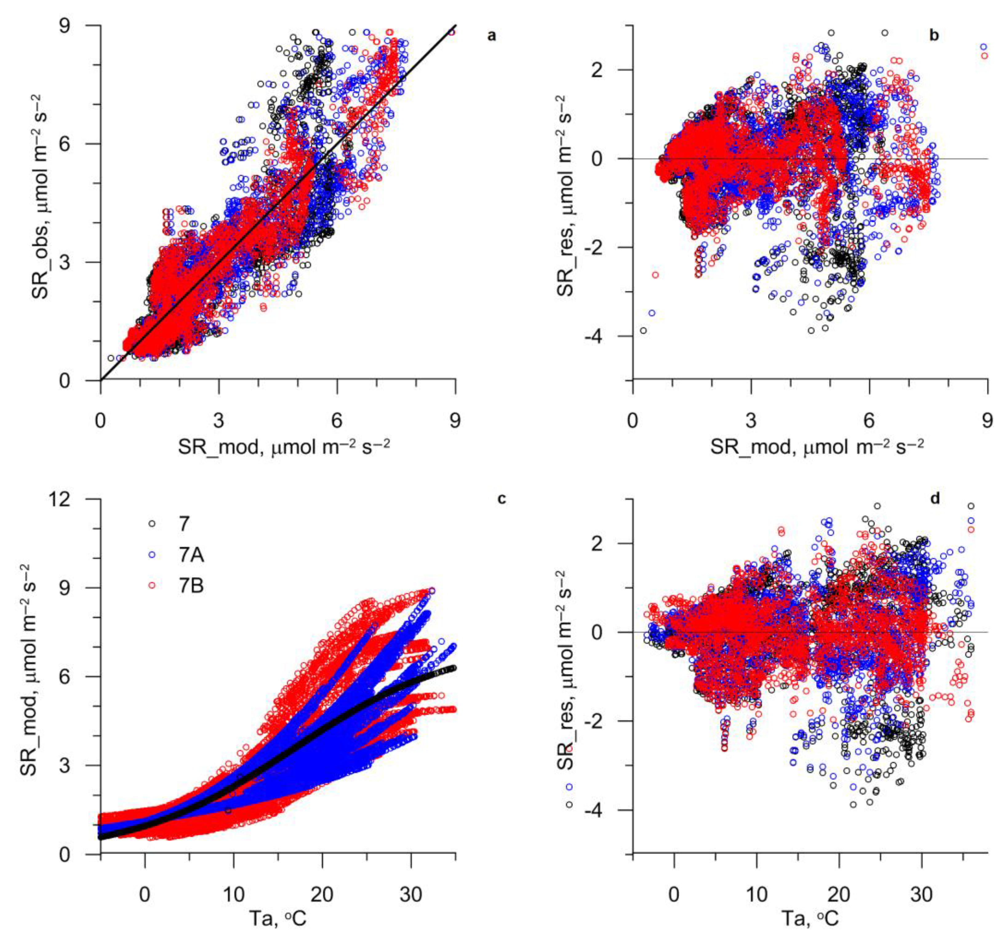
According to the comparison of the model efficiencies (NSE, MAE, and RMSE), the best equations describing soil respiration fluxes were the exponential and logistic models with linear model parameter dependences on soil temperature (models 3B and 7B). The measured and simulated CO2 effluxes and model residuals for the logistic models (models 7, 7A, and 7B) are presented in Figure 5. Panels a and b in Figure 5 show the ability of the models to predict the fluxes. The observed and modeled data are located along the 1:1 line. The basic models underestimated the maximum soil effluxes, and this bias was reduced by modifications. The maximum model residual decreased from 3.88 to 3.48 and then to 2.62 µmol/m2/s when applying modification A and then B, while the MAE values were approximately five times lower (0.73, 0.63, and 0.54 µmol/m2/s, respectively).

Figure 5.
Relationship between observed (SR_obs) CO2 soil effluxes and model residuals (SR_res) against modeled effluxes (SR_mod) and air temperatures (Ta) for the logistic model (model 7) with modifications A and B. Solid line is a 1:1 line in panel a and a zero line in panels b and d.
As shown in Figure 5c, the CO2 efflux obtained by the base logistic model (model 7) was functionally related to the air temperature. The soil respiration simulations according to model 7A exhibited a set of logistic-type curves describing the changes in soil respiration with air temperature at various soil temperatures. Model modification B caused spreading of a range of logistic-type curves, but their shape remained intact. The absence of a systematic error in the models is claimed by almost zero dependence of the model residuals, both from air temperature and soil respiration (Figure 5b,d). Similar relationships were observed for all investigated models (see Supplementary Materials).
Considering the dependence of model parameters on soil temperature (modifications A and B) significantly increased the accuracy of the modeling approach. The mean soil CO2 efflux for the growing season obtained using the modified logistic model (7B) was 2.44 ± 1.67 µmol/m2/s. The estimated mean, minimum, and maximum CO2 flux values were 2.44, 0.57, and 8.91 µmol/m2/s, respectively (Table 5).
4. Discussion
4.1. Observed CO2 Fluxes
The root exclusion method was used to measure heterotrophic respiration at the bare soil site. The bare soil site was trenched six months before the beginning of the soil respiration measurement to reduce the artificial impact of trenching [43]. The vegetation at the site was thoroughly cut in September 2013, and large roots were extracted from the surface layer. There was no soil digging to ensure that the soil compaction and inner structure were maintained, so some fine roots remained in the soil. Fine root decomposition could have caused an overestimation of heterotrophic respiration of up to 14% [44]. The measured soil CO2 effluxes at the trenched bare soil site represent the heterotrophic respiration fluxes, and total soil respiration typically includes HR and root respiration.
The modeled CO2 efflux rate was 2.4 µmol/m2/s for the growing season of 2014 (Table 5). This estimate is similar to those previously reported. The measured heterotrophic respiration fluxes are close to those measured for European grasslands [45], where the maximum soil respiration rates range from 1.9 to 15.9 µmol/m2/s. The annual variations in soil respiration in a semiarid temperate grassland in Inner Mongolia range from 0.5 to 8.0 µmol/m2/s, depending on the land management system [39], and are within the limits obtained in this study. The CO2 emission rates of a Southern Californian grassland are 1.6 µmol/m2/s [46], which is consistent with the emissions from other semiarid grasslands (for example, Wang et al. [39] measured an average of 2.1 µmol/m2/s). Higher soil respiration rates have been measured at managed grassland sites in Finland (peak values of 11.6–25 µmol/m2/s; seasonal average 1.82–7.95), with the higher values recorded in peat soils, and the lower values in sandy and clayey soils [47]. Grassland fertilization enhances soil respiration. An increase in the annual total soil respiration of 24–57% was measured in the first year after fertilization under semiarid temperate climate conditions [48]. The growing season soil respiration in urban areas is much greater [49], and soils in urban forests, lawns, and landscaped areas in the residential areas of Boston emit 2.62, 4.49, and 6.73 ± 0.26 μmol/m2/s, respectively.
The pulsed behavior of soil respiration (Figure 4) can be explained by the joint influence of fast and slow temperature responses [17] or the impact of soil moisture conditions on soil CO2 efflux [50]. Long-term drought stress influences soil CO2 effluxes, which has reduced heterotrophic respiration at a trenched site in the tropical rainforest of Southwest China [51].
Urban areas are significant contributors to global carbon dioxide emissions, but only a limited number of studies have been conducted on CO2 fluxes using micrometeorological or chamber techniques [49,52,53]. The soil chamber measurements of a treeless vegetation surface in Helsinki indicated that the soil respiration level ranged from 1 to 3 µmol/m2/s [52]. Decina et al. [49] found that soil respiration is much higher in urban areas during the growing season, with a rate of 4.49 ± 0.14 µmol/m2/s in urban lawns. These rates were 2.2 times higher than those in nearby rural ecosystems.
4.2. Soil Respiration Models
The response of soil respiration to temperature has been described by a wide variety of empirical models [1,2] with different theoretical bases; however, relatively few studies [11,16,54] have examined how multiple models might fit various in situ soil respiration data, and none of these models are applicable across a wide range of ecosystems or climates. Reichstein and Beer [2] provided an overview of modeling approaches to soil respiration, discussed the dependencies of soil respiration on various environmental factors, and summarized the most important challenges to consider when analyzing soil respiration.
The Lloyd and Taylor and Gamma models were consistently better for explaining soil respiration fluxes in a boreal black spruce plantation than the linear and Q10 models [11]. Khomnik et al. [16] demonstrated that the Gamma model was either better than or as good as the Q10, Lloyd and Taylor, and logistic models in five forest ecosystems spanning three different climate zones, i.e., boreal, temperate, and the Mediterranean. Rodeghiero and Cescatti [17] described a regression model that based the short-term response of soil respiration to soil temperature on the logistic equation, and the logistic equation parameters were related to the environmental variables influencing long-term and site-specific variability.
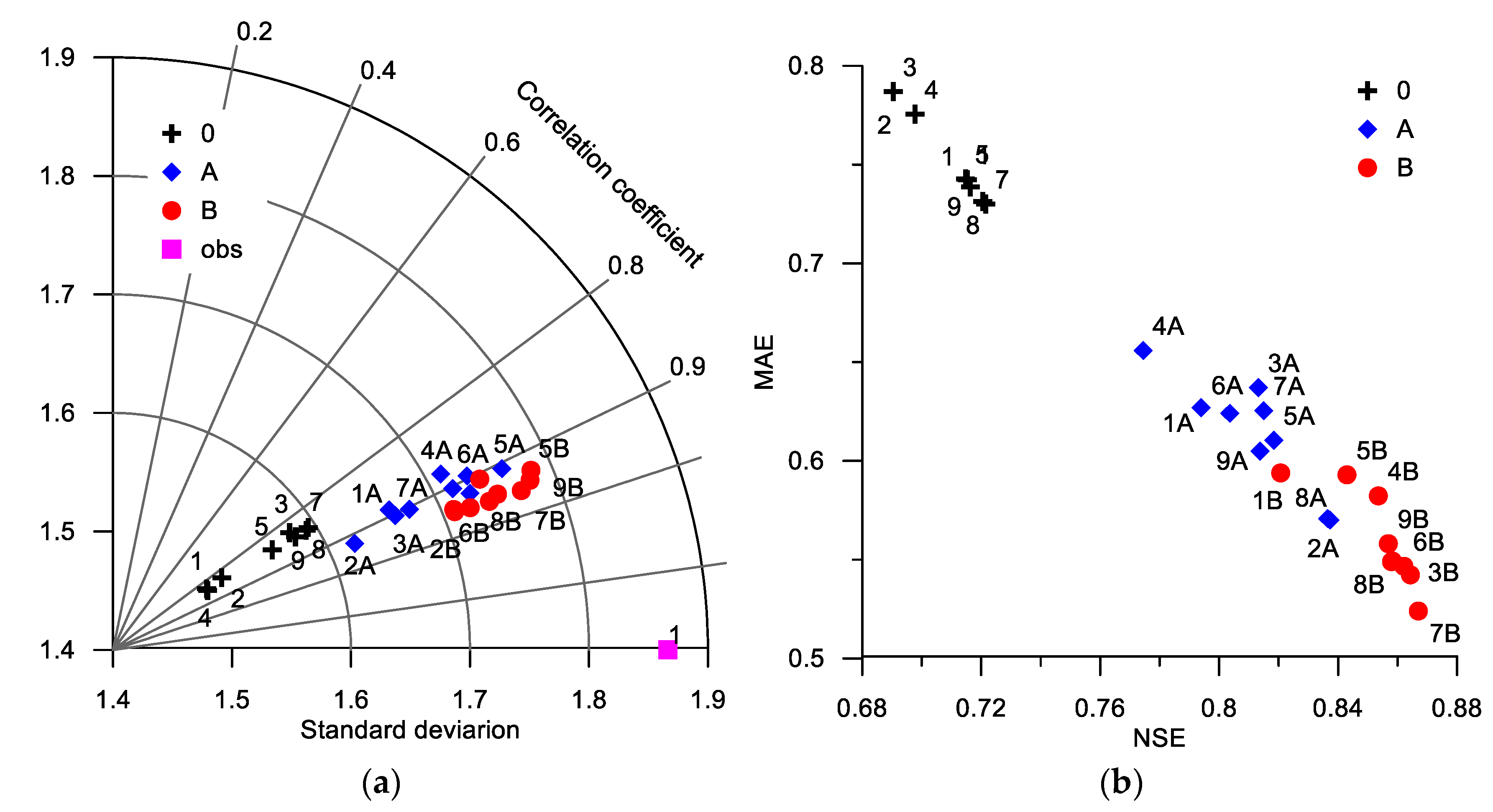
This study tested the performance of nine models (Table 1) in reproducing the temporal variability of soil respiration fluxes. It was demonstrated that air temperature explained slightly more variability than surface or soil temperature. The short-term responses of soil respiration to changes in temperature were well-expressed by the base models (see Table 1). Air temperature was used as a variable for controlling soil respiration in all studied models. According to Singh et al. [55], a MAE of <50% of the standard deviation of the observed data can be considered low. The standard deviation of the observed soil respiration was 1.87 µmol/m2/s; therefore, all nine base models could reproduce the soil CO2 effluxes well (Figure 6). The logistic (model 8), sigmoid (model 7), and Gamma (model 9) models exhibited the best results in describing short-term variations in soil respiration.
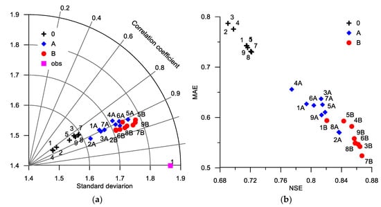
Figure 6.
Taylor diagram (a) and model goodness characteristics (NSE) (b) for base (0) and modified (A,B) soil respiration models. Obs: observation data (STD = 1.87).
A review of the soil respiration fluxes [56] showed that several parameters influence soil emission-related processes. Microbial activity, root respiration, chemical decay processes, and the heterotrophic respiration of soil fauna and fungi produce greenhouse gases in soils [57]. The related emission fluxes largely depend on the soil water content [10,50,58], temperature [59,60], nutrient availability, microbial biomass [9], and community [29], pH [61], and land cover-related parameters [62]. The moisture conditions primarily determine seasonal CO2 emission values at pine forests on sandy soils [10] or a meadow steppe in Inner Mongolia [4], while on bare soil the moisture content does not significantly affect the CO2 efflux [63]. Therefore, meteorological and climatological parameters, as well as land-use management information, are vital [56]. When analyzing seasonal variations in soil respiration, several of the factors affecting respiration co-vary. For example, biological activity is higher in the summer and adds on to the “pure” or direct temperature response [2,9]. The diagnostic carbon flux model [64] suggests that the rate of base ecosystem respiration at the reference temperature is not a constant and depends on the aboveground biomass and gross primary productivity. The relationship between the observed in situ soil respiration rates and soil temperature cannot be easily determined as soil respiration originates at different depths, with each having its own temperature dynamics [2]. D’Angelo et al. [26] demonstrated that the temporal delays between ecosystem respiration and soil temperature in peat soils at different depths are significant at a daily timescale. The time-shifted signals can be used to improve the representation of ecosystem respiration by a model using daily timescale synchronization. The temperature sensitivity determined from the Q10 model depends on the depth and the ecosystem type [65], resulting in more subsoil C vulnerable to loss with increasing temperature.
The soil respiration temperature sensitivity and the base level of respiration are controlled by several closely related factors [14,56], such as microbial activity and biomass, soil moisture content, atmospheric pressure, near-surface wind speed, freeze–thaw transition, O2 content, pH, soil carbon and nitrogen, and nutrients’ availability. Most of these factors followed an apparent seasonal pattern, with changes alongside the seasonal changes in air temperature. The seasonal variations in soil temperature were also shifted and were smoother than the seasonal variations in air temperature (Table 2). The deep-layer soil temperature can be used as a formal variable for describing variations in other environmental characteristics controlling soil respiration [65]. Bauer et al. [66] demonstrated that different temperature response function formulations resulted in estimated response factors that deviated over the range of soil water content, and for temperatures below 25 °C, very little. Wohlfahrt and Galvagno [67] used a linear combination of air and soil temperatures to describe the observed hysteresis relationship between ecosystem respiration and temperature, while Hibbard et al. [68] analyzed soil respiration across the northern hemisphere temperate ecosystem and found that including soil moisture could improve the correlation, but not significantly. Zhou et al. [69] found that the combined function of soil temperature and moisture did not fit the data well under severe water stress, while Jassal et al. [70] stated that, in an 18-year-old temperate Douglas fir stand, soil respiration is positively correlated with soil temperature at a depth of 2 cm under a high soil water content at a depth of 4 cm; however, under a low soil water content, soil respiration was largely decoupled from soil temperature. This suggests that, under different environmental conditions, the appropriate representation of some specific soil respiration processes may change [28,54].
In this study, considering soil temperatures in a respiration model always improved the model fit (indicated by R, MAE, and NSE; Figure 6). The Taylor diagram representing the model performance demonstrated that the modified models matched the soil efflux observations well. The correlations between the observed and modeled results were close to 0.84 for the base models, 0.9 for model modification A, and 0.92 for model modification B. The simulation results of the modified models exhibited higher standard deviation values than the base model, but those of models 5B and 9B were closer to the standard deviations of the observation data. The mean absolute error decreased from 0.73–0.79 to 0.57–0.66 µmol/m2/s and 0.52–0.59 µmol/m2/s after applying model modifications A and B, respectively (Figure 6b). Soil respiration model 7B exhibited the lowest MAE of 0.52 µmol/m2/s. This indicates that model–data disagreement can be largely reduced by using soil temperature-dependent model parameters instead of a fixed value. Site-specific and non-stationary model parameters are important in regional simulations of carbon fluxes [17,71].
4.3. Apparent Temperature Sensitivity Coefficient, Q10
Soil respiration models generally apply a fixed Q10 coefficient as the power function between soil respiration and temperature [13]. In addition to the temperature sensitivities of the enzymatic affinity to the substrate and the diffusion of the substrate to the enzyme, the supply of substrate via active translocation can covary with the temperature and the season [72]. The apparent Q10 of soil respiration may be the sum or product of various responses to the increasing temperature. Other studies indicated that Q10 varies between ecosystems and across temperature ranges, which may be because the various components of soil respiration have different temperature sensitivities [73,74].
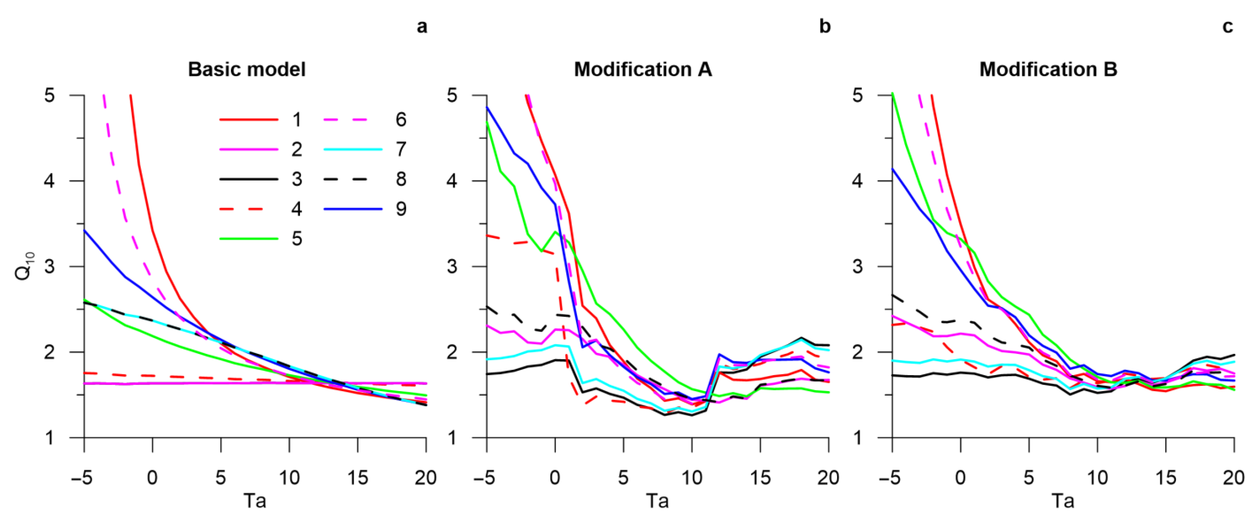
We also examined the apparent temperature sensitivity (described by the Q10 coefficient; Equation (3)) of the soil respiration models (Table 1). We applied the method used in previous studies to determine the Q10 values [75,76] for each model by dividing the predicted values across a 10 °C range. For example, Q10 for 5 °C was computed as soil respiration at 15 °C divided by soil respiration at 5 °C. The Q10 values depend on the controlling temperatures [66,77,78], and the dependencies of the Q10 values on air temperature for the base models are shown in Figure 7a. According to the definitions (Table 1), Q10 does not depend on temperature for models 2 and 3, with values of 1.64 and 1.68, respectively. The changes in Q10 with increases in air temperature obtained for the Arrhenius model (model 4) were lower than those for all the other models. The simulations conducted using models 5–9 demonstrated a gradual decrease in Q10 from 2.18–2.48 at 0 °C to 1.38–1.49 at +20 °C. The average Q10 values were low (1.64–1.68) for models 2, 3, and 4, moderate (1.89–2.02) for models 1, 5, 7, and 8, and high (2.11 and 2.44) for models 6 and 9. The linear model (model 1) exhibited an extremely high apparent temperature sensitivity coefficient at low air temperatures (line 1 in Figure 7).
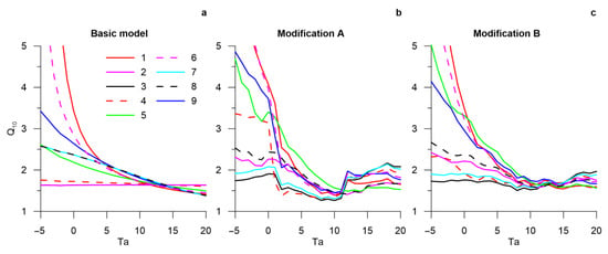
Figure 7.
Relationships between the apparent temperature sensitivity, Q10, and air temperatures (Ta) for base models 1–9 and their modifications, A and B.
The explicit temperature dependence of the temperature sensitivity coefficient (Equation (1)) implemented in model modification A increased the variability of the Q10 values. The average values of Q10 for the models with modification A were 2.5% (model 1A) to 22.9% (model 5A) higher than those for the base models, excluding models 7A and 7B, where the average Q10 values decreased by 9.6% and 4.8%, respectively. The apparent temperature sensitivity values under negative air temperatures were high for models 1, 6, 9, 4A, and 5A. The Q10 values for air temperature ranging from +2 to +10 °C were lowest for all the studied models as the explicit changes in temperature sensitivity during the growing season correlated with changes in soil temperature. Model modification B smoothed the shape of the temperature dependencies of the Q10 values. The average values of Q10 were comparable to those obtained for model modification A, excluding model 4B, which exhibited 8.3% lower Q10 values, and model 9B, which exhibited 9.6% higher Q10 values. The average Q10 values were low (1.72–1.83) for models 3B, 4B, and 7B, moderate (1.90–2.05) for models 1B, 2B, and 8B, and high (2.32–2.65) for models 5, 6, and 9. The Q10 value of the model with the best performance (logistic model 7B) was 1.78 ± 0.12 and did not significantly vary with changes in air temperature (Figure 7c).
It is important to note that Q10 values calculated using various models did not significantly differ for an air temperature range from 10 to 20 °C, and they are comparable with estimations obtained in other studies. For example, Q10 estimated in a clear-cut in the Southern Taiga was about 2.21 [79]. Q10 values for ecosystem respiration were in a range of 2.36 to 2.61 for an alpine meadow ecosystem of a permafrost site on the Qinghai-Tibetan Plateau, and warming increased the Q10 values [33]. Q10 values ranging between 1.63 and 1.74 were obtained for semiarid, temperate-climate grassland in Inner Mongolia, depending on the fertilization system [48]. Contrary to previous findings, Mahecha et al. [23] suggest that the Q10 is independent of mean annual temperature, does not differ among biomes, and is confined to values around 1.4 ± 0.1. Several authors have empirically noted that Q10 declines with the increasing temperature, with a particular focus on respiration [35,73]. Schipper et al. [80] explained the raised Q10 at low temperatures using macromolecular thermodynamic theory. The observed increase of the apparent temperature sensitivity, Q10, at temperatures of about 0 °C was likely related to the intensification of the soil respiration during freezing–thawing events [81,82]. Davidson et al. [32] speculate that apparent Q10 values of respiration that are significantly above about 2.5 probably indicate that some unidentified process of substrate supply is confounded with the observed temperature variation.
Our findings suggest that the apparent Q10 sensitivity coefficient can widely vary and depends on the temperature sensitivity model used. The Q10 model does not reflect the actual relationships between soil respiration and temperature. The apparent Q10 values must be carefully interpreted, particularly with respect to soil respiration.
5. Conclusions
The modified soil CO2 efflux models calibrated using observation data allowed us to estimate the net growing season carbon emissions. Soil respiration modeling demonstrated that the apparent temperature sensitivity coefficient significantly varied. Soil respiration in Equation (1) represents the fast response of respiration to environmental characteristics. The revealed relationships between soil respiration parameters and soil/air temperature (Figure 1) were characterized by slow long-term processes in microbial biomass development [9,29,83]. The fast and slow responses of soil respiration contribute to the pulsed behavior [17]. However, a high soil temperature often coincides with low moisture availability, which confounds the response of soil CO2 efflux to temperature [50]. The goodness-of-fit (RMSE, MAE, NSE) of the models suggested that the modified models can be used to estimate CO2 effluxes from soils and provide a better understanding of the contribution of the soil ecosystem to the carbon cycle in urban environments. According to the efficiency of the models, the best equations describing the soil respiration fluxes were the exponential and logistic models with linear dependencies of the model parameters on soil temperatures (models 3B and 7B). The base models underestimated the maximum soil effluxes, but this bias was reduced by model modifications. The aspects of the environmental control of soil respiration highlighted in this study, particularly the joint effects of soil temperature and the shape of the temperature response function, may aid the future development of mechanistic models for the responses of soil to global warming.
Supplementary Materials
The following supporting information can be downloaded at: https://www.mdpi.com/article/10.3390/land12050939/s1, Figure S1: NSE coefficient for models’ modification B at various combinations of governing temperatures T2 and T3. Figure S2: Relationship of observed (SR_obs) CO2 soil effluxes and model residuals (SR_res) with modeled effluxes (SR_mod) and air temperatures (Ta) for base and modified models.
Author Contributions
Conceptualization, E.A.D.; methodology, E.A.D.; formal analysis, E.A.D. and S.A.K.; investigation, E.A.D. and S.A.K.; resources, E.A.D. and S.A.K.; data curation, E.A.D. and S.A.K.; writing—original draft preparation, E.A.D. and S.A.K.; writing—review and editing, E.A.D.; visualization, S.A.K.; supervision, E.A.D. All authors have read and agreed to the published version of the manuscript.
Funding
This model development and testing was carried out as part of the most important innovative project of national importance: “Development of a system for ground-based and remote monitoring of carbon pools and greenhouse gas fluxes in the territory of the Russian Federation, ensuring the creation of recording data systems on the fluxes of climate-active substances and the carbon budget in forests and other terrestrial ecological systems” (#123030300031-6). In situ observations and raw data processing were supported by the Russian Academy of Sciences within the framework of the state assignment of the Institute of Monitoring of Climatic and Ecological System Siberian Branch of the Russian Academy of Sciences.
Data Availability Statement
The data discussed in this paper are available upon request.
Conflicts of Interest
The authors declare no conflict of interest.
References
- Kudeyarov, V.N. Soil respiration and biogenic carbon dioxide sink in the territory of Russia: An analytical review. Eurasian Soil Sci. J. 2018, 51, 599–612. [Google Scholar] [CrossRef]
- Reichstein, M.; Beer, C. Soil respiration across scales: The importance of a model-data integration framework for data interpretation. J. Plant Nutr. Soil Sci. 2008, 171, 344–354. [Google Scholar] [CrossRef]
- IPCC. Climate Change 2021: The Physical Science Basis; Contribution of Working Group I to the Sixth Assessment Report of the Intergovernmental Panel on Climate, Change; Masson-Delmotte, V., Zhai, P., Pirani, A., Connors, S.L., Péan, C., Berger, S., Caud, N., Chen, Y., Goldfarb, L., Gomis, M.I., et al., Eds.; Cambridge University Press: Cambridge, UK; New York, NY, USA, 2021; 2391p. [Google Scholar]
- Wang, X.; Fan, K.; Yan, Y.; Chen, B.; Yan, R.; Xin, X.; Li, L. Controls of Seasonal and Interannual Variations on Soil Respiration in a Meadow Steppe in Eastern Inner Mongolia. Agronomy 2023, 13, 20. [Google Scholar] [CrossRef]
- Azizi-Rad, M.; Guggenberger, G.; Ma, Y.; Sierra, C.A. Sensitivity of soil respiration rate with respect to temperature, moisture and oxygen under freezing and thawing. Soil Biol. Biochem. 2022, 165, 108488. [Google Scholar] [CrossRef]
- Zeeshan, M.; Wenjun, Z.; Chuansheng, W.; Yan, L.; Azeez, P.A.; Qinghai, S.; Yuntong, L.; Yiping, Z.; Zhiyun, L.; Liqing, S. Soil heterotrophic respiration in response to rising temperature and moisture along an altitudinal gradient in a subtropical forest ecosystem, Southwest China. Sci. Total Environ. 2022, 816, 151643. [Google Scholar] [CrossRef]
- Suleau, M.; Moureaux, C.; Dufranne, D.; Buysse, P.; Bodson, B.; Destain, J.P.; Heinesch, B.; Debacq, A.; Aubinet, M. Respiration of three Belgian crops: Partitioning of total ecosystem respiration in its heterotrophic, above- and below-ground autotrophic components. Agric. For. Meteorol. 2011, 151, 633–643. [Google Scholar] [CrossRef]
- Kurganova, I.N.; Lopes de Gerenyu, V.O.; Khoroshaev, D.A.; Myakshina, T.N.; Sapronov, D.V.; Zhmurin, V.A.; Kudeyarov, V.N. Analysis of the long-term soil respiration dynamics in the forest and meadow cenoses of the Prioksko-Terrasny biosphere reserve in the perspective of current climate trends. Eurasian Soil Sci. 2020, 53, 1421–1436. [Google Scholar] [CrossRef]
- Čapek, P.; Starke, R.; Hofmockel, K.S.; Bond-Lamberty, B.; Hess, N. Apparent temperature sensitivity of soil respiration can result from temperature driven changes in microbial biomass. Soil Biol. Biochem. 2019, 135, 286–293. [Google Scholar] [CrossRef]
- Makhnykina, A.V.; Prokushkin, A.S.; Menyailo, O.V.; Verkhovets, S.V.; Tychkov, I.I.; Urban, A.V.; Rubtsov, A.V.; Koshurnikova, N.N.; Vaganov, E.A. The Impact of Climatic Factors on CO2 Emissions from Soils of Middle-Taiga Forests in Central Siberia: Emission as a Function of Soil Temperature and Moisture. Russ. J. Ecol. 2020, 51, 46–56. [Google Scholar] [CrossRef]
- Bond-Lamberty, B.; Bailey, V.L.; Chen, M.; Gough, C.M.; Vargas, R. Globally rising soil heterotrophic respiration over recent decades. Nature 2018, 560, 80–83. [Google Scholar] [CrossRef]
- Arrhenius, S. Über die Reaktionsgeschwindigkeit bei der Inversion von Rohrzucker durch Säuren. Z. Für Phys. Chem. 1889, 4, 226. [Google Scholar] [CrossRef]
- van’t Hoff, J.H. Lectures on Theoretical and Physical Chemistry. Part 1: Chemical Dynamics; Lehfeldt, R.A., Translator; Edward Arnold: London, UK, 1898. [Google Scholar]
- Ali, R.S.; Poll, C.; Kandeler, E. Dynamics of soil respiration and microbial communities: Interactive controls of temperature and substrate quality. Soil Biol. Biochem. 2018, 127, 60–70. [Google Scholar] [CrossRef]
- Rowson, J.G.; Worrall, F.; Evans, M.G. Predicting soil respiration from peatlands. Sci. Total Environ. 2013, 442, 397–404. [Google Scholar] [CrossRef] [PubMed]
- Khomik, M.; Altaf Arain, M.; Liaw, K.L.; McCaughey, J.H. Debut of a flexible model for simulating soil respiration-soil temperature relationship: Gamma model. J. Geophys. Res. Biogeosci. 2009, 114, G03004. [Google Scholar] [CrossRef]
- Rodeghiero, M.; Cescatti, A. Main determinants of forest soil respiration along an elevation/temperature gradient in the Italian Alps. Glob. Change Biol. 2005, 11, 1024–1041. [Google Scholar] [CrossRef]
- Reichstein, M.; Falge, E.; Baldocchi, D.; Papale, D.; Aubinet, M.; Berbigier, P.; Bernhofer, C.; Buchmann, N.; Gilmanov, T.; Granier, A.; et al. On the separation of net ecosystem exchange into assimilation and ecosystem respiration: Review and improved algorithm. Glob. Change Biol. 2005, 11, 1424–1439. [Google Scholar] [CrossRef]
- Fang, C.; Moncrieff, J.B. The dependence of soil CO2 efflux on temperature. Soil Biol. Biochem. 2001, 33, 155–165. [Google Scholar] [CrossRef]
- Lloyd, J.; Taylor, J.A. On the temperature dependence of soil respiration. Funct. Ecol. 1994, 8, 315–323. [Google Scholar] [CrossRef]
- Jenkinson, D.S. The turnover of organic carbon and nitrogen in soil. Philos. Trans. R. Soc. Lond. Ser. B Biol. Sci. 1990, 329, 361–368. [Google Scholar]
- Richards, F.J. A flexible growth function for empirical use. J. Exp. Bot. 1959, 10, 290–300. [Google Scholar] [CrossRef]
- Mahecha, M.D.; Reichstein, M.; Carvalhais, N.; Lasslop, G.; Lange, H.; Seneviratne, S.I.; Vargas, R.; Ammann, C.; Arain, M.A.; Cescatti, A.; et al. Global convergence in the temperature sensitivity of respiration at ecosystem level. Science 2010, 329, 838–840. [Google Scholar] [CrossRef] [PubMed]
- Kuzyakov, Y. Sources of CO2 efflux from soil and review of partitioning methods. Soil Biol. Biochem. 2006, 38, 425–448. [Google Scholar] [CrossRef]
- Subke, J.A.; Bahn, M. On the ‘temperature sensitivity’ of soil respiration: Can we use the immeasurable to predict the unknown? Soil Biol. Biochem. 2010, 42, 1653–1656. [Google Scholar] [CrossRef] [PubMed]
- D’Angelo, B.D.; Gogo, S.; Laggoun-Défarge, F.; Moing, F.; Jégou, F.; Guimbaud, C. Soil temperature synchronisation improves representation of diel variability of ecosystem respiration in Sphagnum peatlands. Agric. For. Meteorol. 2016, 223, 95–102. [Google Scholar] [CrossRef]
- Luo, Y.; Zhou, X. Controlling factors. In Soil Respiration and the Environment; Luo, Y., Zhou, X., Eds.; Academic Press: Burlington, MA, USA, 2006; pp. 79–105. [Google Scholar] [CrossRef]
- Swails, E.; Hertanti, D.; Hergoualc’h, K.; Verchot, L.; Lawrence, D. The response of soil respiration to climatic drivers in undrained forest and drained oil palm plantations in an Indonesian peatland. Biogeochemistry 2019, 142, 37–51. [Google Scholar] [CrossRef]
- Ma, Y.; McCormick, M.K.; Szlavecz, K.; Filley, T.R. Controls on soil organic carbon stability and temperature sensitivity with increased aboveground litter input in deciduous forests of different forest ages. Soil Biol. Biochem. 2019, 134, 90–99. [Google Scholar] [CrossRef]
- Wang, Y.; Song, C.; Yu, L.; Mi, Z.; Wang, S.; Zeng, H.; Fang, C.; Li, J.; He, J.S. Convergence in temperature sensitivity of soil respiration: Evidence from the Tibetan alpine grasslands. Soil Biol. Biochem. 2018, 122, 50–59. [Google Scholar] [CrossRef]
- Golovatskaya, E.A.; Dyukarev, E.A. The influence of environmental factors on the CO2 emission from the surface of oligotrophic peat soils in West Siberia. Eurasian Soil Sci. J. 2012, 45, 588–597. [Google Scholar] [CrossRef]
- Davidson, E.A.; Janssens, I.A. Temperature sensitivity of soil carbon decomposition and feedbacks to climate change. Nature 2006, 440, 165–173. [Google Scholar] [CrossRef]
- Qin, Y.; Yi, S.; Chen, J.; Ren, S.; Wang, X. Responses of ecosystem respiration to short-term experimental warming in the alpine meadow ecosystem of a permafrost site on the Qinghai-Tibetan Plateau. Cold Reg. Sci. Technol. 2015, 115, 77–84. [Google Scholar] [CrossRef]
- Kirschbaum, M.U.F. The temperature dependence of organic-matter decomposition—Still a topic of debate. Soil Biol. Biochem. 2006, 38, 2510–2518. [Google Scholar] [CrossRef]
- Hamdi, S.; Moyano, F.; Sall, S.; Bernoux, M.; Chevallier, T. Synthesis analysis of the temperature sensitivity of soil respiration from laboratory studies in relation to incubation methods and soil conditions. Soil Biol. Biochem. 2013, 58, 115–126. [Google Scholar] [CrossRef]
- Dyukarev, E.A. Partitioning of net ecosystem exchange using chamber measurements data from bare soil and vegetated sites. Agric. For. Meteorol. 2017, 239, 236–248. [Google Scholar] [CrossRef]
- LI-COR Biosciences: LI-8100A Automated Soil CO2 Flux System & LI-8150 Multiplexer Instruction Manual. 2010. Available online: http://envsupport.licor.com/docs/LI-8100A_Manual.pdf (accessed on 16 January 2023).
- Kiselev, M.V.; Voropay, N.N.; Dyukarev, E.A.; Kurakov, S.A.; Kurakova, P.S.; Makeev, E.A. Automatic meteorological measuring systems for microclimate monitoring. IOP Conf. Ser. Earth Environ. Sci. 2018, 190, 012031. [Google Scholar] [CrossRef]
- Wang, Z.; Ji, L.; Hou, X.; Schellenberg, M.P. Soil respiration in semiarid temperate grasslands under various land management. PLoS ONE 2016, 11, e0147987. [Google Scholar]
- Mahadevan, P.; Wofsy, S.C.; Matross, D.M.; Xiao, X.; Dunn, A.L.; Lin, J.C.; Gerbig, C.; Munger, J.W.; Chow, V.Y.; Gottlieb, E.W. A satellite-based biosphere parameterization for net ecosystem CO2 exchange: Vegetation photosynthesis and respiration model (VPRM). Glob. Biogeochem. Cycles 2008, 22, GB2005. [Google Scholar] [CrossRef]
- Kurganova, I.N.; Lopes de Gerenyu, V.O.; Myakshina, T.N.; Sapronov, D.V.; Kudeyarov, V.N. CO2 emission from soils of various ecosystems of the Southern Taiga zone: Data analysis of continuous 12-year monitoring. Doklady Biol. Sci. 2011, 1, 56–58. [Google Scholar] [CrossRef]
- Nash, J.E.; Sutcliffe, J.V. River flow forecasting through conceptual models. Part I—A discussion of principles. J. Hydrol. 1970, 10, 282–290. [Google Scholar] [CrossRef]
- Savage, K.E.; Davidson, E.A.; Abramoff, R.Z.; Finzi, A.C.; Giasson, M.A. Partitioning soil respiration: Quantifying the artifacts of the trenching method. Biogeochemistry 2018, 140, 53–63. [Google Scholar] [CrossRef]
- Díaz-Pinés, E.; Schindlbacher, A.; Pfeffer, M.; Jandl, R.; Zechmeister-Boltenstern, S.; Rubio, A. Root trenching: A useful tool to estimate autotrophic soil respiration? A case study in an Austrian mountain forest. Eur. J. For. Res. 2010, 129, 101–109. [Google Scholar] [CrossRef]
- Bahn, M.; Rodeghiero, M.; Anderson-Dunn, M.; Dore, S.; Gimeno, C.; Drösler, M.; Williams, M.; Ammann, C.; Berninger, F.; Flechard, C.; et al. Soil respiration in European grasslands in relation to climate and assimilate supply. Ecosystems 2008, 11, 1352–1367. [Google Scholar] [CrossRef] [PubMed]
- Aronson, E.L.; Goulden, M.L.; Allison, S.D. Greenhouse gas fluxes under drought and nitrogen addition in a Southern California grassland. Soil Biol. Biochem. 2019, 131, 19–27. [Google Scholar] [CrossRef]
- Lohila, A.; Aurela, M.; Regina, K.; Laurila, T. Soil and total ecosystem respiration in agricultural fields: Effect of soil and crop type. Plant Soil 2003, 251, 303–317. [Google Scholar] [CrossRef]
- Peng, Q.; Dong, Y.; Qi, Y.; Xiao, S.; He, Y.; Ma, T. Effects of nitrogen fertilization on soil respiration in temperate grassland in Inner Mongolia, China. Environ. Earth Sci. 2011, 62, 1163–1171. [Google Scholar] [CrossRef]
- Decina, S.M.; Hutyra, L.R.; Gately, C.K.; Getson, J.M.; Reinmann, A.B.; Short Gianotti, A.G.; Templer, P.H. Soil respiration contributes substantially to urban carbon fluxes in the greater Boston area. Environ. Pollut. 2016, 212, 433–439. [Google Scholar] [CrossRef]
- Jia, X.; Zha, T.S.; Wu, B.; Zhang, Y.Q.; Gong, J.N.; Qin, S.G.; Chen, G.P.; Qian, D.; Kellomäki, S.; Peltola, H. Biophysical controls on net ecosystem CO2 exchange over a semiarid shrubland in northwest China. Biogeosciences 2014, 11, 4679–4693. [Google Scholar] [CrossRef]
- Zhou, L.; Liu, Y.; Zhang, Y.; Sha, L.; Song, Q.; Zhou, W.; Balasubramanian, D.; Palingamoorthy, G.; Gao, J.; Lin, Y.; et al. Soil respiration after six years of continuous drought stress in the tropical rainforest in Southwest China. Soil Biol. Biochem. 2019, 138, 107564. [Google Scholar] [CrossRef]
- Vesala, T.; Järvi, L.; Launiainen, S.; Sogachev, A.; Rannik, Ü.; Mammarella, I.; Siivola, E.; Keronen, P.; Rinne, J.; Riikonen, A.; et al. Surface–atmosphere interactions over complex urban terrain in Helsinki, Finland. Tellus B 2008, 60, 188–199. [Google Scholar] [CrossRef]
- Kordowski, K.; Kuttler, W. Carbon dioxide fluxes over an urban park area. Atmos. Environ. 2010, 23, 2722–2730. [Google Scholar] [CrossRef]
- Chen, X.; Post, W.M.; Norby, R.J.; Classen, A.T. Modeling soil respiration and variations in source components using a multi-factor global climate change experiment. Clim. Change 2011, 107, 459–480. [Google Scholar] [CrossRef]
- Singh, J.; Knapp, H.V.; Arnold, J.G.; Demissie, M. Hydrologic modeling of the Iroquois River watershed using HSPF and SWAT. J. Am. Water Res. Assoc. 2005, 41, 361–375. [Google Scholar] [CrossRef]
- Oertel, C.; Matschullat, J.; Zurba, K.; Zimmermann, F.; Erasmi, S. Greenhouse gas emissions from soils—A review. Geochem. 2016, 76, 327–352. [Google Scholar] [CrossRef]
- Chapuis-Lardy, L.; Wrage, N.; Metay, A.; Chotte, J.L.; Bernoux, M. Soils, a sink for N2O? A review. Glob. Change Biol. 2007, 13, 1–17. [Google Scholar] [CrossRef]
- Tucker, C.L.; McHugh, T.A.; Howell, A.; Gill, R.; Weber, B.; Belnap, J.; Grote, E.; Reed, S.C. The concurrent use of novel soil surface microclimate measurements to evaluate CO2 pulses in biocrusted interspaces in a cool desert ecosystem. Biogeochemistry 2017, 135, 239–249. [Google Scholar] [CrossRef]
- Kurganova, I.N.; Lopes de Gerenyu, V.O. Contribution of abiotic factors to CO2 emission from soils in the freeze–thaw cycles. Eurasian Soil Sci. J. 2015, 48, 1009–1015. [Google Scholar] [CrossRef]
- Osipov, A.F. Effect of interannual difference in weather conditions of the growing season on the CO2 emission from the soil surface in the middle-taiga cowberry–lichen pine forest (Komi republic). Eurasian Soil Sci. J. 2018, 51, 1419–1426. [Google Scholar] [CrossRef]
- Ludwig, J.; Meixner, F.X.; Vogel, B.; Förstner, J. Soil-air exchange of nitric oxide: An overview of processes, environmental factors, and modeling studies. Biogeochemistry 2001, 52, 225–257. [Google Scholar] [CrossRef]
- Liu, Y.; He, N.; Zhu, J.; Xu, L.; Yu, G.; Niu, S.; Sun, X.; Wen, X. Regional variation in the temperature sensitivity of soil organic matter decomposition in China’s forests and grasslands. Glob. Change Biol. 2017, 23, 3393–3402. [Google Scholar] [CrossRef]
- Juhász, C.; Huzsvai, L.; Kovács, E.; Kovács, G.; Tuba, G.; Sinka, L.; Zsembeli, J. Carbon Dioxide Efflux of Bare Soil as a Function of Soil Temperature and Moisture Content under Weather Conditions of Warm, Temperate, Dry Climate Zone. Agronomy 2022, 12, 3050. [Google Scholar] [CrossRef]
- Xiao, J.F.; Davis, K.J.; Urban, N.M.; Keller, K.; Saliendra, N.Z. Upscaling car- bon fluxes from towers to the regional scale: Influence of parameter variability and land cover representation on regional flux estimates. J. Geophys. Res. Atmos. 2011, 116, G00J06. [Google Scholar] [CrossRef]
- Li, J.; Yan, D.; Pendall, E.; Pei, J.; Noh, N.J.; He, J.S.; Li, B.; Nie, M.; Fang, C. Depth dependence of soil carbon temperature sensitivity across Tibetan permafrost regions. Soil Biol. Biochem. 2018, 126, 82–90. [Google Scholar] [CrossRef]
- Bader, C.; Müller, M.; Schulin, R.; Leifeld, J. Peat decomposability in managed organic soils in relation to land use, organic matter composition and temperature. Biogeosciences 2018, 15, 703–719. [Google Scholar] [CrossRef]
- Wohlfahrt, G.; Galvagno, M. Revisiting the choice of the driving temperature for eddy covariance CO2 flux partitioning. Agric. For. Meteorol. 2017, 237–238, 135–142. [Google Scholar] [CrossRef]
- Hibbard, K.A.; Law, B.F.; Reichstein, M.; Sulzman, J. An analysis of soil respiration across northern hemisphere temperate ecosystems. Biogeochemistry 2005, 73, 29–70. [Google Scholar] [CrossRef]
- Zhou, X.; Wan, S.; Luo, Y. Source components and interannual variability of soil CO2 efflux under experimental warming and clipping in a grassland ecosystem. Glob. Change Biol. 2007, 13, 761–775. [Google Scholar] [CrossRef]
- Jassal, R.S.; Black, T.A.; Novak, M.D.; Gaumont-Guay, D.; Nesic, Z. Effect of soil water stress on soil respiration and its temperature sensitivity in an 18-year-old temperate Douglas-fir stand. Glob. Change Biol. 2008, 14, 1305–1318. [Google Scholar] [CrossRef]
- Qiu, C.; Zhu, D.; Ciais, P.; Guenet, B.; Krinner, G.; Peng, S.; Aurela, M.; Bernhofer, C.; Brümmer, C.; Bret-Harte, S.; et al. ORCHIDEE-PEAT (revision 4596), a model for northern peatland CO2, water, and energy fluxes on daily to annual scales. Geosci. Mod. Dev. 2018, 11, 497–519. [Google Scholar] [CrossRef]
- Davidson, E.A.; Janssens, I.A.; Lou, Y. On the variability of respiration in terrestrial ecosystems: Moving beyond Q10. Glob. Change Biol. 2006, 12, 154–164. [Google Scholar] [CrossRef]
- Kirschbaum, M.U.F. The temperature-dependence of soil organic matter decomposition, and the effect of global warming on soil organic C storage. Soil Biol. Biochem. 1995, 27, 753–760. [Google Scholar] [CrossRef]
- Carrasco, J.J.; Neff, J.C.; Harden, J.W. Modeling physical and biogeochemical controls over carbon accumulation in a boreal forest soil. J. Geophys. Res. Biogeosci. 2006, 111, G02004. [Google Scholar] [CrossRef]
- Hogg, E.H.; Lieffers, V.J.; Wein, R.W. Potential carbon losses from peat profiles: Effects of temperature, drought cycles, and fire. Ecol. Appl. 1992, 2, 298–306. [Google Scholar] [CrossRef]
- Hardie, S.M.L.; Garnett, M.H.; Fallick, A.E.; Rowland, A.P.; Ostle, N.J.; Flowers, T.H. Abiotic drivers and their interactive effect on the flux and carbon isotope (14C and δ13C) composition of peat-respired CO2. Soil Biol. Biochem. 2011, 43, 2432–2440. [Google Scholar] [CrossRef]
- Jiang, J.; Guo, S.; Zhang, Y.; Liu, Q.; Wang, R.; Wang, Z.; Li, N.; Li, R. Changes in temperature sensitivity of soil respiration in the phases of a three-year crop rotation system. Soil Tillage Res. 2015, 150, 139–146. [Google Scholar] [CrossRef]
- Fierer, N.; Colman, B.P.; Schimel, J.P.; Jackson, R.B. Predicting the temperature dependence of microbial respiration in soil: A continental-scale analysis. Glob. Biogeochem. Cycles 2006, 20, GB3026. [Google Scholar] [CrossRef]
- Mamkin, V.; Kurbatova, J.; Avilov, V.; Ivanov, D.; Kuricheva, O.; Andrej, V.; Yaseneva, I.; Olchev, A. Energy and CO2 exchange in an undisturbed spruce forest and clear-cut in the Southern Taiga. Agric. For. Meteorol. 2019, 265, 252–268. [Google Scholar] [CrossRef]
- Schipper, L.A.; Hobbs, J.K.; Rutledge, S.; Arcus, V.L. Thermodynamic theory explains the temperature optima of soil microbial processes and high Q10 values at low temperatures. Glob. Change Biol. 2014, 20, 3578–3586. [Google Scholar] [CrossRef]
- Kurganova, I.; Teepe, R.; Loftfield, N. Influence of freeze-thaw events on carbon dioxide emission from soils at different moisture and land use. Carbon Balance Manag. 2007, 2, 2. [Google Scholar] [CrossRef] [PubMed]
- Matzner, E.; Borken, W. Do freeze-thaw events enhance C and N losses from soils of different ecosystems? A review. Eur. J. Soil Sci. 2008, 59, 274–284. [Google Scholar] [CrossRef]
- Janssens, I.A.; Lankreijer, H.; Matteucci, G.; Kowalski, A.S.; Buchmann, N.; Epron, D.; Pilegaard, K.; Kutsch, W.; Longdoz, B.; Grunwald, T.; et al. Productivity overshadows temperature in determining soil and ecosystem respiration across European forests. Glob. Change Biol. 2001, 7, 269–278. [Google Scholar] [CrossRef]
Disclaimer/Publisher’s Note: The statements, opinions and data contained in all publications are solely those of the individual author(s) and contributor(s) and not of MDPI and/or the editor(s). MDPI and/or the editor(s) disclaim responsibility for any injury to people or property resulting from any ideas, methods, instructions or products referred to in the content. |
© 2023 by the authors. Licensee MDPI, Basel, Switzerland. This article is an open access article distributed under the terms and conditions of the Creative Commons Attribution (CC BY) license (https://creativecommons.org/licenses/by/4.0/).

