Article

Simulating Urban Agglomeration Expansion in Henan Province, China: An Analysis of Driving Mechanisms Using the FLUS Model with Considerations for Urban Interactions and Ecological Constraints

School of Geoscience & Technology, Zhengzhou University, Zhengzhou 450001, China
*
Author to whom correspondence should be addressed.
Land 2023, 12(6), 1189; https://doi.org/10.3390/land12061189
Submission received: 9 March 2023 / Revised: 29 May 2023 / Accepted: 31 May 2023 / Published: 6 June 2023
(This article belongs to the Special Issue Future Urban Land Expansion in China)

Abstract

:
Urban expansion is influenced by complex and variable social, economic, natural, and policy-related factors. Given their nonlinear interactions, accurately modeling these urban expansion processes poses a challenge. While most studies treat the city as an independent entity, prioritizing internal urban factors, urban land expansion is influenced by intercity interactions and the ecological environment. This study proposes a new approach that couples the gravitational field model, ecological constraints, and the Future Land Use Simulation (FLUS) model, comprehensively considering the impact of intercity interaction and the ecological environment. The experiment in Henan Province in China assessed the effects of factors such as basic spatial variables (Slope and distance to the city center), urban gravitational field, and ecological constraints on urban expansion through the optimal parameters-based geographical detector (OPGD) model. The feasibility of the method was confirmed by this case study, which shows that it improves the simulation accuracy of the urban agglomeration scale, particularly for central cities. We identified the urban gravitational field and ecological constraints as two important factors affecting the expansion of urban agglomerations. Areas with stronger urban spatial fields are more likely to attract neighboring resources and promote urban expansion, whereas ecological factors constrain the expansion behavior of cities under the condition of ecological and environmental resource protection needs, and both of them work together to influence the expansion behavior of urban clusters. Therefore, we posit that intercity interactions and ecological constraints are important considerations for the future spatial planning of urban agglomerations and for coordinating the harmonious development of urbanization and ecological conservation.

1. Introduction

An urban agglomeration is a highly developed spatial form of an integrated city and is one of the distinguishing features of modern civilization. Defined as an agglomerated radial area comprising one or two core cities and several microcities, an urban agglomeration exhibits close socioeconomic ties. This framework fosters a high level of spatial interaction between cities, contributing to the collective development of a region [1]. However, such high expansion impacts the urban landscape, particularly by significantly reducing ecological and productive space, leading to serious ecological and environmental problems [2,3,4,5]. As the World Commission on Environment and Development (WCED) proposed, national environmental policies and urban development should align with sustainable development goals [6]. Modeling and predicting urban expansion while providing policy-oriented recommendations for the rational control of urban expansion and the coordinated sustainable development of urban ecology have become the focus of current research [7,8,9]. Understanding the relationship between urban expansion and complex networks of urban agglomerations necessitates exploring the mechanisms of urban expansion [10]. This information can further assist policymakers in formulating policy-oriented recommendations [11].
Urban growth is a complex process [12]. Since the emergence of the first theoretical approach to cellular automata (CA)-based models of urban expansion in the 1980s [13], there has been a proliferation of models and methods for simulating urban expansion, which have evolved to the micro-dynamic model stage [9]. Many scholars have developed various land use simulation models to understand better the land use change process under different scenarios. These models include the conversion of land use and its effects at a small regional extent (CLUE-S) model [14], the land-use scenario dynamics (LUSD) model [15], multi-agent system models of land use/cover change (MAS/LUCC models) [16], etc. Among these, the most widely used method is CA, which has successfully explored various urban phenomena. It is widely used to simulate dynamic urban expansion and optimize urban spatial structures [17]. However, its limitation includes its weaknesses in the quantitative aspect and its inability to include the driving forces of urban growth in the simulation process [18]. In contrast, artificial intelligence (AI)-based methods offer the advantage of capturing the nonlinearity and heterogeneity of urban growth. Their improvement over traditional CA has achieved good results in urban growth simulations [19]. Many scholars have simulated land-use dynamics by combining artificial intelligence methods with CA models. For instance, Qiang et al. combined and improved artificial neural networks (ANN) and the CA method to simulate complex LULC dynamics in a vulnerable coastal region with high accuracy [20]. Feng et al. proposed a machine-learning CA model based on a least-squares support vector machine (LS-SVM) to simulate urban growth, which can capture the spatial complexity of urban dynamics and improve simulation accuracy [21]. Liu proposed an urban growth model using a self-adaptive genetic algorithm (SAGA) to optimize (CA), which outperformed the logistics-CA model [22]. Liao et al. proposed a neighbor decay cellular automata model based on particle swarm optimization (PSO-NDCA) with a higher prediction accuracy for built-up land [23]. Urban expansion is influenced by many complex and variable factors, such as social, economic, natural, and policy factors, with high uncertainty levels. This makes it difficult to simulate urban expansion accurately. The future land-use simulation (FLUS) model was proposed by Xiaoping [24], who considered climate, natural, and socioeconomic factors. The model performs top-down system dynamics and bottom-up meta-automata interactions, integrates ANNs, and introduces adaptive competition and inertia mechanisms for land-use simulation. This makes it more accurate than other recognized systems such as CLUE-S and CA, and it has been widely used to simulate and predict land use/cover changes under the influence of human activities and natural conditions [25].
Most current studies use CA to simulate urban expansion, treating the city as an individual entity, favoring internal factors, and ignoring interactions between cities. The interflow of urban space (e.g., the flow of people, transport, and information) is increasingly important in driving urban expansion in metropolitan areas [26,27]. Therefore, it is necessary to consider spatial interactions between cities when modeling large-scale urban expansion [28]. Urban mobility intensity serves as a valid indicator of the intensity of socioeconomic interactions among member cities in metropolitan cluster areas [29,30]. Furthermore, with urbanization, there is a need to scientifically control the scale of cities to coordinate their sustainable development with the surrounding ecological environment [8]. Hence, urban development under ecological constraints is an effective way to address and mitigate the ecological impact of rapid and uncontrolled urbanization [31]. For example, Ma [7] integrated ecological correlation into CA for urban growth simulation, and Li et al. [32] introduced conservation priorities based on standardized values of green infrastructure assessment into CA. They simulated and explored the impact of the ecological environment on the urbanization process to better coordinate the relationship between urban expansion and ecological protection.
In general, current studies incorporating urban interactions and ecological constraints into urban expansion simulations mainly manifest in two ways. For small regional scales, such as individual cities, ecological constraints are primarily incorporated into urban growth boundaries or urban expansion simulations under ecological constraints [6,7,32,33]. These studies consider conflicts between urban expansion and environmental protection. However, studies on urban simulation at a large regional scale of urban agglomerations primarily integrate the interflow effects between cities in urban expansion simulations [28,34] and study the effects of spatial interactions between cities on urban growth.
Although many studies have analyzed the relationship between urban expansion and urban interactions or ecological constraints, few have incorporated both urban interactions and ecological constraints into urban agglomeration expansion simulations. While gradually promoting urban development, it is also necessary to reduce the negative impact of urban expansion on the ecological environment. Therefore, considering the dual factors of ecological constraints and urban interactions is necessary for studying urban agglomeration expansion.
Simultaneously, analyzing urban agglomeration expansion patterns and driving mechanisms has gradually become a hot research topic [35], and scholars posit that natural, transportation location, socioeconomic, and policy factors are the main factors driving urban expansion [36,37,38,39]. However, the driving factors of urban growth and their influences vary in different regions and development stages [40]. Understanding the main determinants of regional urban sprawl can help planners formulate more locality-oriented measures to control urban expansion in an orderly manner [38].
In summary, this study constructs a new approach to land use simulation that couples gravitational field models and ecological constraints to incorporate urban interactions and ecological constraints as driving variables in urban expansion simulation models. First, urban strength and flow data were integrated to calculate urban spatial field strength. Although prior studies [28,34,41] have utilized gravitational field models to measure the strength of spatial interactions between cities, as intercity flows play an increasingly important role in the evolution of urban agglomerations [27,28], the individual flow indicators of cities cannot fully reflect the spatial interactions that occur between them. Therefore, this study integrates human, traffic, and information flow data between cities and calculates cities’ comprehensive gravitational spatial field strength by combining the time–cost distance. Then, the ecological quality of the region was comprehensively evaluated from two perspectives: the remote sensing ecological index (RSEI) and the ecological resistance surface (ERS) of urban expansion, which is taken as the ecological constraint of urban expansion. Finally, the FLUS model incorporates the gravitational field model and ecological constraints into the conversion rules of the FLUS model to predict the conversion probability of urban units more accurately. The feasibility of this study’s methodology was verified by simulating the land-use dynamics of an intercity cluster in Henan Province and exploring the individual and coupled effects of the different drivers measured using the optimal parameters-based geographical detector (OPGD) model. This study provides rational suggestions for controlling urban expansion and coordinating sustainable development in both society and nature.

2. Research Methodology

This study proposes an urban expansion simulation framework coupling the gravitational field model and ecological constraints based on the FLUS model (Figure 1). This framework is divided into five main steps:
  • Selection of basic spatial variables. Based on extensive research related to the FLUS model and previous studies on the land-use status of urban agglomerations, we selected ten drivers that significantly impact land-use change for this study;
  • Construction of a gravitational field model that integrates socioeconomic data, other statistical data, and flow data, such as the Baidu index, population migration, traffic flow, and time–cost distance. We designated the urban spatial interaction intensity as a driving factor for the demand-driven FLUS model, subsequently simulating urban expansion in metropolitan areas;
  • Evaluation of ecological quality. Ecological quality was assessed using the RSEI and ERS coefficients, and this was used to determine the restricted development area, which was set as a constraint for the expansion of urban clusters;
  • Creation of a coupled model for urban agglomeration expansion simulation experiments. The accuracy of the simulation results was evaluated using the model validation method;
  • Analysis of the driving mechanism of urban agglomeration expansion. Factor analysis and interaction analysis were performed for each driver using the OPGD model.

2.1. Gravitational Field Model

Urban flows typically include bidirectional interchanges in population, information, technologies, and goods among cities, which may affect the growth and spatial patterns of hierarchical cities. From the perspective of each city, urban flows can be divided into urban inflows and flows. Urban inflows reflect the cumulative effects of urban energy, whereas urban outflows represent spillover effects. This study considers urban flows as a driver of urban land development, linking urbanization to land change over large geographical distances, aiming to consider the evolution of individual land cells and urban flows between different cities in urban agglomerations.
In proposing the gravity model, physicist Stewart was inspired by Newton’s formula for universal gravitation [42], which Reilly [42] applied to study intercity retail markets. As its application has expanded, more scholars have utilized it to study urban spatial structure changes. The gravity model is expressed as follows:
I i , j = G Q i Q j r i j β
where I i , j is the gravitational force of cities i and j, r i j is the distance between the two cities, Q i , Q j is a socioeconomic measure (e.g., population or GDP), G is the gravitational force coefficient, and β is the gravitational decay index.
However, the gravitational force model expresses the magnitude of the force acting between two points. Guo et al. [43] argued that the nature of this force lies in the existence of a gravitational potential field, akin to the universal gravitational potential field, at the center of each city through which two cities or regions interact. Researchers have measured urban interactions in a spatially explicit manner by constructing a gravitational field [44]:
U i , x , y = F i D x , y , x i , y i β
where U i , x , y are the spatial field intensities of the pixels (x, y) subjected to the image of the city i, F i is the urban influence of city i, and D x , y , x i , y i is the distance of the pixels (x, y) from the center of city i x i , y i .
A single indicator (population, GDP, etc.) is not sufficient to fully reflect a city’s influence; therefore, a comprehensive system of indicators (Table 1) was constructed to evaluate the size of a city’s influence. The equation is expressed as follows:
F i = k = 1 m W k P k
where F i is the overall influence size of the city, W k refers to the weight value of the k-th factor influencing the city’s power, using the entropy weighting method to determine the weight size of each indicator, P k refers to the score size of the k-th factor influencing the city’s power, P k 0 , 100 , and m is the number of the types of factors (X1, X2, …, X15).
W k = 1 + l n n 1 i = 1 n P i j l n P i j k = 1 m 1 + l n n 1 i = 1 n P i j l n P i j
P i j   = X i j   i = 1 n X i j  
where X i j   denotes the score of factor j of the city i, i = 1 n X i j   denotes the score of factor j of the city i, and n denotes the number of cities.
Urban spatial interactions in the context of metropolitan areas, such as urban agglomerations, can be quantified through urban spatial field intensities. However, urban agglomerations are intricate systems, and relying on one or two city flow indicators alone cannot adequately capture their spatial interactions. In this study, intercity flow data encompassing human, traffic, and information flows were comprehensively measured to construct an intercity contact intensity matrix, which was utilized to assess the spatial field intensity. The calculation of the spatial field intensity was carried out using the following formula:
F L i , j = k = 1 m λ k × R i j k
where F L i , j is the combined urban flow from city i to city j, λ k is the weight of the k-th elemental flow, R i j k is the normalized flow from city i to city j, and m is the number of the types of elemental flows.
λ k = 1 + K i = 1 n × n P l k l n P l k k = 1 m 1 + K i = 1 n × n P l k l n P l k ,   K = 1 / l n n × n
P l k = R i j k i = 1 , J = 1 n R i j k ,   l = i × j
R i j k = X i j k i = 1 n X i j k
where P l k is the contribution of the l-th data point of the k-th element, X i j k is the urban flow from city i to city j, i = 1 n X i j k is the total outflow of element k from city i, and n indicates the number of cities.
Considering the conservative nature of the data flow, the combined inflow F L i , j i n and outflow F L i , j o u t of the city were calculated.
Spatial interactions between cities are relatively independent, and together, they influence regional development. Therefore, the cumulative effect is used to determine the effect of urban flows on cells (x, y) in the city i. The final gravitational field model is expressed as follows:
U i , x , y i n = F i D x , y , x i , y i β × F L i , j i n
U i , x , y o u t = F i D x , y , x i , y i β × F L i , j o u t
where U i , x , y i n denotes the total urban inflow of city i to grid (x, y) in the city i, U i , x , y o u t denotes the total urban outflow of the city i to grid (x, y) in the city i, and F i denotes the composite city strength index. F L i , j i n is the total inflow to the city i, F L i , j o u t is the total outflow from the city I, and β is the distance decay index, with a value of 2.
The cost distance is also used instead of the Euclidean distance, where D denotes the cost distance. Speeds were allocated to different modes of travel and land use types. These were: 120 km/h for highways, 100 km/h for railways, 80 km/h for national roads, 60 km/h for provincial roads, 40 km/h for county roads, 30 km/h for built-up land, and 10 km/h for non-built-up land.
c o s t = S i z e   o f   g r i d   c e l l s S p e e d   o f   t r a v e l × 60

2.2. Ecological Quality Assessment

The RSEI and ERS of urban expansion were used to evaluate the quality of the ecological environment and as an ecological constraint on urban expansion. The RSEI provides an objective measure of regional ecological conditions, while the ERS coefficient indicates the challenges associated with managing and incorporating other urban landscapes.

2.2.1. RSEI

RSEI is an indicator initially proposed and applied by Xu Hanqiu [45]. It facilitates visual assessment of the ecological environment by considering various factors such as the normalized difference vegetation index (NDVI), WET, land surface temperature (LST), and normalized differential build-up and bare soil index (NDBSI). This comprehensive approach allows for a holistic representation of the regional ecological environment. The calculation function for RSEI is as follows:
R S E I 0 = 1 P C A 1 N D V I , W E T , N D B S I , L S T
R S E I = R S E I 0 R S E I 0 m i n R S E I 0 m a x R S E I 0 m i n
where P C A 1 is the principal component analysis. The closer the R S E I value is to 1, the better the ecological quality, and vice versa.

2.2.2. ERS

Urban expansion is a process of competition for controlling urban landscapes relative to other landscapes, and this control and coverage must be achieved by overcoming resistance [9]. The RSEI objectively assesses regional ecological conditions, while the surface resistance coefficient of ERS reflects the difficulty of controlling urban landscapes and covering other landscapes. This study chose the built-up area at the city center point as the source of ecological resistance to urban expansion. Factors such as soil erodibility, soil erosion sensitivity, biodiversity service function, water conservation service function, soil and water conservation service function, land use type, and slope were considered resistance factors. The weight for each factor was determined using hierarchical analysis. The minimum cumulative resistance model (MCR) was then employed to calculate ecological resistance values and generate an ecological resistance surface for urban expansion. The specific calculations were as follows:
(1) Soil erosion sensitivity:
S i = R × K × L S × P V 4
where S i is the sensitivity index for soil erosion, R is the rainfall erosion force (MJ·mm·hm−2·h−1), K is the soil erodibility (t·m−2), L S is the slope length and factor, and P V is the vegetation coverage (%).
(a) Rainfall erosion force:
R = i = 1 12 E I i
E I i = 73.989 × P i 2 P a 0.7387
where E I i is the average monthly rainfall erosion force; P i is the rainfall during the ith month; and P a is the average annual rainfall. The average annual rainfall erosion force is the sum of the monthly rainfall erosion force values for a year.
(b) Slope length and slope factor:
L S = L × S
L = λ 22.13 m
m = B B + 1
B = sin θ 3 sin θ 0.8 + 0.56
S = 10.8 × sin θ + 0.036 ,     θ < 5 16.8 × sin θ 0.5 ,     5 θ < 10 21.9 × sin θ 0.96 ,     θ 10
where S is the slope factor, L is the slope length factor, θ is the slope, λ is the slope length, and m is the slope length index.
(c) Vegetation coverage:
P V = N D V I N D V I s o i l N D V I v e g N D V I s o i l
where, P V is the vegetation coverage value of the image element, N D V I is the vegetation index value of the mixed-image element, N D V I s o i l is the vegetation index value of the pure vegetation image element, and N D V I v e g is the vegetation index value of the pure soil image element. Here [46], the value with a cumulative frequency of 5% in the N D V I annual maximum synthetic frequency accumulation table is denoted as N D V I v e g , and the value with a cumulative frequency of 95% in the N D V I annual maximum synthetic frequency accumulation table is denoted as N D V I s o i l .
(2) Biodiversity service function:
S b i o = N P P m e a n × F p r e × F t e m × 1 F a l t
where S b i o is the service capacity of biodiversity, N P P m e a n is the average annual net primary productivity of vegetation (g C·m−2·a−1), F p r e is the average annual precipitation (mm), F t e m is the average annual temperature (°C), and F a l t is the elevation factor (m).
(3) Water conservation service function:
W R = N P P m e a n × F s i c × F p r e × 1 F s l o
where W R is the water conservation capacity index of the ecosystem, F s l o is the degree of relief of the land surface, and F s i c is the soil seepage.
(4) Soil and water conservation service function:
S p e o = N P P m e a n × 1 K × 1 F s l o
where S p e o is the soil and water conservation.
(5) Land use type and slope resistance values (Table 2):
(6) Minimum cumulative resistance model:
M C R = f m i n j = n i = m D i j · R i
where M C R is the minimum cumulative resistance model, f   is a function reflecting the positive relationship between M C R and the variables D i j and R i , D i j is the spatial distance of the ecological source from j across i, and R i is the resistance value across the landscape surface i.

2.3. Future Land Use Simulation (FLUS) Model

2.3.1. Introduction to the Model

The FLUS model, based on the CA principle proposed by Liu [24], is a comprehensive model that integrates an artificial neural network (ANN) algorithm and a roulette wheel selection mechanism derived from the stochastic dynamic (SD) and CA models. The model’s fundamental principle involves estimating the development probability of each land-use category within a region. This estimation is achieved by utilizing each driver’s base period land-use data and data through an artificial neural network algorithm. The development probability is then combined with the domain influence factor, adaptive inertia coefficient, and conversion cost to determine the overall conversion probability of each meta-cell. Subsequently, the simulation results are obtained using the roulette wheel competition mechanism.
The FLUS model facilitates the effective coupling of human and natural influences to simulate various land use scenarios. It enhances the performance of multiple land use and land cover change modeling. As a result, the FLUS model has gained wide application for simulating and predicting land use/cover changes influenced by human activities and natural conditions [25]. It is particularly suitable for complex land-use simulations involving multiple scenarios, multiple scales, and high accuracies [47].

2.3.2. FLUS Model Parameter Settings

(1) Prediction of the scale of future land demand
The total future land use demand represents the total number of pixels occupied by each land use type during the forecast period. This study used the Markov Chain method to forecast the total number of pixels for each land use type in 2030, based on the land use type data from 2020, using the following equation:
S t + 1 = P i j × S t
where S t and S t + 1 are the state matrices of the land at moments t and t + 1, respectively, and P i j denotes the probability of transformation from site type i to site type j.
(2) Neighborhood impact factor setting
The neighborhood impact factor is an indicator that captures the interaction between different site types and sites within a neighborhood. It is expressed as a dimensionless value ranging from 0 to 1, with values closer to 1 indicating a stronger expansion of the specific land use type. Wang et al. [48] demonstrated that the dimensionless values of the Total Area (TA) variation satisfy the requirements of neighborhood weights in the FLUS model in terms of both parameter significance and data structure. In this study, their calculation method is referred to in order to determine the final domain weight values. However, the weight values are adjusted to ensure they fall between 0.5 and 1.0, thus avoiding zero weight values. The formula used for this adjustment is as follows:
T A i = j = 1 n a i j 1 10000
W O i = T A i m i n T A i m a x T A i m i n T A i  
W i = W 0 i 2 + 0.5
where n is the number of patches, a is the area of the patches, W O i is the dimensionless value of the T A change, and W i is the final domain weight value.
(3) Conversion cost matrix:
The cost matrix refers to the rules of change between land types and indicates whether land types can be converted into each other. Considering the realities of land-use change and the economic costs and technical conditions of interconversion between land types (such as the fact that built-up land cannot be converted to other land types), the following land-type conversion matrix was developed (Table 3). In this conversion matrix, 0 means that no interconversion is possible, and 1 means that interconversion is possible.

2.4. The OPGD Model

The geodetector, initially proposed by Wang Jinfeng [49], is a computational model used to explain spatial heterogeneity and analyze the statistical aspects of its underlying driving mechanisms. It has gained widespread use in studying the driving mechanisms behind spatial differentiation [50,51,52]. The OPGD model [53] is an enhancement of the geodetector that aims to find the maximum q-value of continuous variables through different parameter combinations of discretization methods and interval numbers. This model can be flexibly applied in exploring spatial factors and conducting heterogeneity analysis on various spatial data types.
The central concept of this study is based on the assumption that if an independent variable (e.g., DEM or slope) significantly influences the dependent variable (attitudes toward urban land use dynamics), the spatial distribution of the independent and dependent variables should exhibit similarities [54,55]. Therefore, the OPGD model was employed in this study to measure the degree of similarity and analyze the driving mechanisms behind urban land-use change. The calculation of urban land-use dynamics was performed as follows:
k L = L n L m S × 1 t × 100 %
where k L is the dynamic attitude of a land-use type during the study period, L n is the area of a land-use type at the end of the study period, L m is the area of a land-use type at the beginning of the study period, t is the period of land-use change, and S is the area of the study unit.

3. Study Area and Data

3.1. Overview of the Study Area

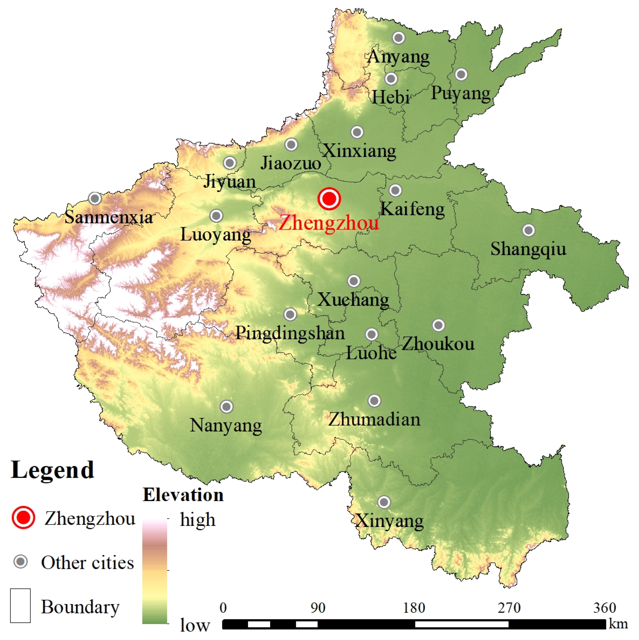
Henan Province is situated in central China, spanning the middle and lower reaches of the Yellow River (110°21′–116°39′ E, 31°23′–36°22′ N). The province features a diverse topography, with higher elevations in the west and lower elevations in the east. It falls within the transitional zone between the high-soil plateau and the North China Plain. The eastern-central region of Henan Province comprises the alluvial plain of the Yellow Huaihai Sea, while the Nanyang Basin occupies the southwestern part. The northern, western, and southern regions are characterized by the Taihang, Fuyu, Tongbai, and Dabie Mountains, respectively, which are rich in ecological resources.
Henan Province holds strategic importance as a transportation hub in China, serving as the intersection of multiple national highways and railways. The province has experienced rapid development in recent years, undergoing significant industrialization and urbanization. As per the Henan Province New Urbanization Plan (2021–2035), in addition to optimizing the “1 + 8” spatial pattern with Zhengzhou as the primary city, there is a focus on promoting and cultivating the growth and influence of sub-centers such as Luoyang and Nanyang. The plan also emphasizes the acceleration of constructing a development pattern that involves one main center, two sub-centers, four synergistic zones, and multiple support points, resulting in a complex urban ecosystem structure. The location of Henan Province is illustrated in Figure 2.

3.2. Data Sources and Processing

The spatial dataset required for this study consists of three main components: basic data, gravitational field model data, and ecological constraint data (Table 4).
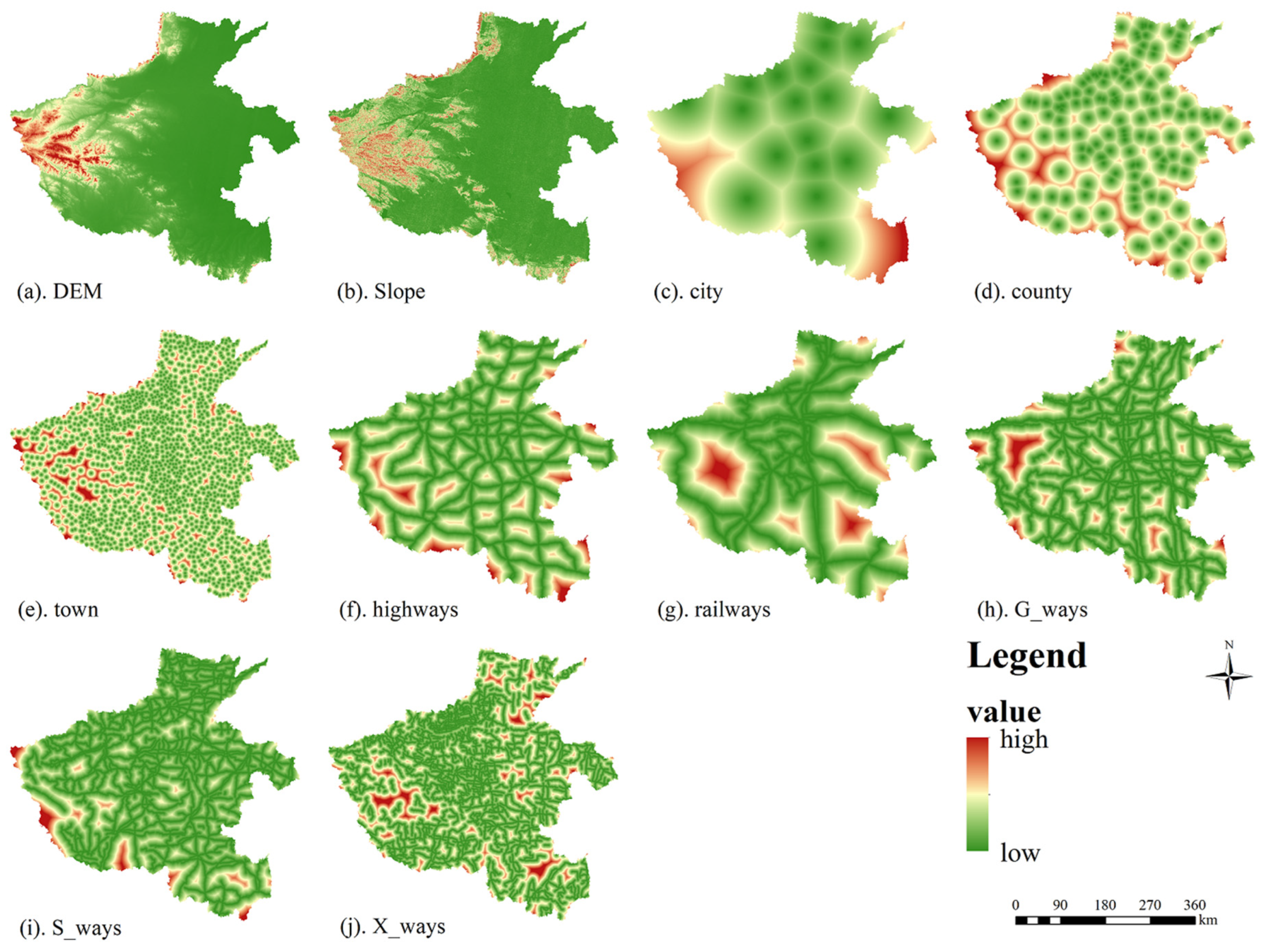
First, we extracted administrative boundaries, city points, district and county points, township points, highways, railways, national roads, provincial roads, and county roads from basic geospatial data downloaded from the National Geomatics Center of China. The DEM and land use type data (2010 and 2020) were mosaicked and masked to extract the slope data using DEM calculations, and all data were resampled to a 100 m resolution for ease of calculation. The DEM, slope, distance from different urban centers (city centers, district and county centers, and town centers), and distance from other types of roads (highways, railways, national roads, provincial roads, and county roads) were chosen as the basic spatial variables to measure the probability of urban land expansion (Figure 3).
The flow data were then calculated. The flow data (people, information, and traffic flow) were set up as two-way flow data from city A as the starting point to city B, forming a data flow intensity matrix between the two cities. In addition, each city’s influence evaluation index statistics were obtained from the Henan Provincial Statistical Yearbook.
Finally, we used a calculation method for indicators related to ecological quality assessment to obtain the RSEI and ERS.

4. Results and Analysis

4.1. Urban Spatial Field Strength

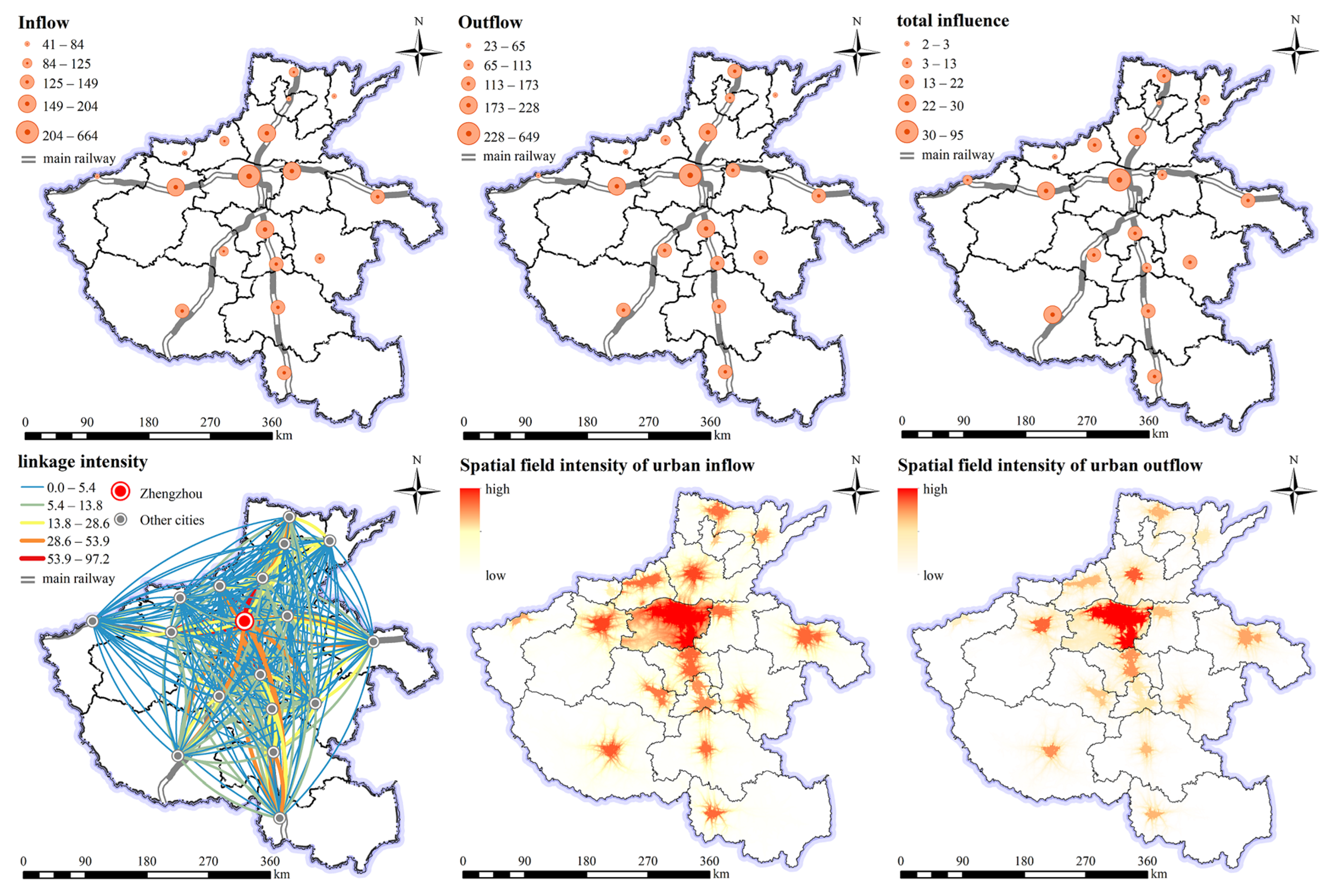
Statistical data obtained for each city’s influence evaluation indicator were used to determine the weight of each indicator. This was performed using the entropy weighting method to calculate the final comprehensive city influence. The collected 18 × 18 matrix data for the people, traffic, and information flows were used to determine the weight values for each type of flow data using the entropy weighting method. In this study, cars and trains were weighed at a 0.5:1 ratio to obtain the final traffic flow data and calculate the combined flow data. Figure 4 shows the distribution of the combined inflows, outflows, total influence, and intercity linkage intensity for each city, indicating that the central city of Zhengzhou has the strongest linkage intensity with other cities. Finally, the spatial gravitational field intensity of the city is calculated according to the gravitational field model described in Section 2.1. As shown in Figure 4, the cities differed slightly, with Zhengzhou exhibiting the highest inflow and outflow intensities.

4.2. Comprehensive Evaluation of Ecological Constraints

Landsat-8 image data were used to calculate each index, and images of the annual means (May–October) were synthesized using the Gee platform code. The final RSEI values were obtained using principal component analysis, as shown in Figure 5a–e.
This study used the method described in Section 2.2.2 to calculate the ecological resistance values for generating urban expansion, as shown in Figure 5f–m.
RSEI and ERS were categorized into five levels using the natural break method. Areas identified as having the best ecological quality and the highest ecological resistance value to urban expansion should not be developed but should instead be dedicated to ecological conservation; thus, values of 0 and 1 were set as restricted areas (Figure 5n). A value of 0 indicates that the area is not allowed to undergo land type conversion, and a value of 1 indicates that conversion is allowed.

4.3. Simulation Accuracy Assessment

The underlying spatial data were used to evaluate the potential for land expansion. Furthermore, the urban spatial gravitational field was used as spatial interaction data to drive urban land expansion, ecological quality was evaluated using RSEI and ERS and was used as a constraint on urban land expansion, and the areas of restricted development were where urban land conversion was not possible. In this study, experiments were conducted using FLUS software, and the field factor weights for each land-use type are listed in Table 5.
Figure 6A shows the results of the urban land use simulations for 2010–2020 for different coupling scenarios of the model. There were four scenarios in total: (a) base FLUS model simulation results (land-use simulations using only the base spatial variables), (b) coupled gravitational field model simulation results, (c) coupled ecological constraint simulation results, and (d) coupled gravitational field models and ecological constraint simulation results.
By comparing the simulation results of five representative cities (Zhengzhou, Luoyang, Xinxiang, Shangqiu, and Xinyang) with those of different cities, it was found that the impact of varying coupling cases was greater for core cities than for non-core cities. The incorporation of inter-urban interaction forces and ecological constraints results in a significant increase in urban land use and a more compact agglomeration, especially in urban areas with a high intensity of urban gravitational fields. By evaluating the simulation results using kappa coefficients, overall accuracy, and Figure of Merit (FOM) metrics (Table 6), it is clear that the inclusion of the urban gravitational field model has a relatively insignificant improvement in overall accuracy, whereas the inclusion of the ecological constraint results in a significant improvement in the accuracy of the model. One reason for this may be that the strength of the urban gravitational field is higher mainly in the built-up areas of the city center; therefore, there is a greater drive for the expansion of built-up land closer to the city center, which is better modeled. In contrast, the ecological environment plays a greater role further away from the city center and is better modeled for discrete urban sites away from the city center. This can lead to an improvement in overall accuracy when the urban gravitational field model is added at the overall level, which does not yield a significant improvement.
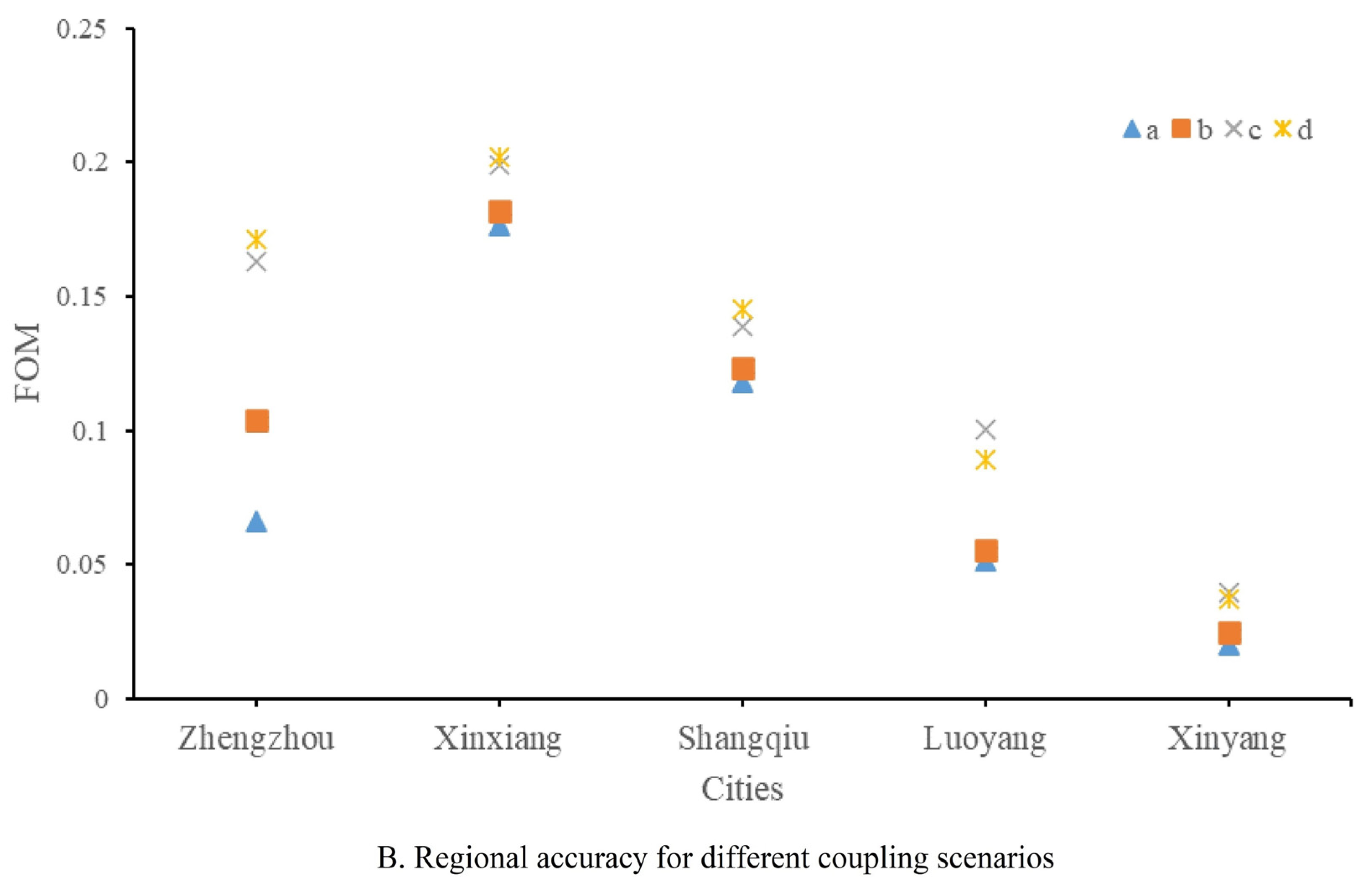
To further validate the abovementioned idea, the regional FOM accuracy was validated for five cities: Zhengzhou, Xinxiang, Shangqiu, Luoyang, and Xinyang, as shown in Figure 6. For regional land-use simulations, the accuracy of the three urban areas of Zhengzhou, Xinxiang, and Shangqiu improved significantly with the coupled gravitational field model, whereas the highest regional simulation was achieved when both the gravitational field and ecological constraints were considered. It is noteworthy that the cities of Luoyang and Xinyang decreased in FOM accuracy after considering both factors compared to when only ecological constraints were considered, which exceeded what was expected. Considering the land-use types and locations of the two areas, it can be seen that they have abundant land-use types, are geographically located in mountains and water, and are rich in ecological resources. This may have created a serious “potential gap” between ecological constraints and inter-urban gravitational drivers, with ecological factors taking absolute precedence, ultimately reducing the overall accuracy. In summary, land-use simulation by coupling the gravitational field model and ecological constraints proposed in this study can improve the model’s performance not only in the entire Henan Province but also in some local areas.

4.4. Simulation of Urban Expansion for 2020–2030

The Markov chain model was used to predict the number of urban land-use types within Henan Province in 2030, and the coupled gravitational field model and ecologically constrained FLUS model were used to predict changes in land use in Henan Province in the same year. Calculating the change in the urban and non-urban land use areas in Henan Province from 2010 to 2030 showed that urban land use increased from 2010 to 2030, reaching an urban land demand of 28,268.83 km2 in Henan Province by 2030 under both urban interactions and ecological constraints. Figure 7 shows the distribution of various land-use types modeled for Henan Province in 2030. It can be seen that the rate of urban land expansion is greater in developed urban areas and that most of the increase in urban land use comes at the expense of decreasing arable land owing to the saturation of built-up space. Due to ecological constraints, there is less urban expansion in areas of high ecological quality, mainly on the western and southern fringes. The results showed that inter-urban interaction forces and ecological condition constraints incorporated into urban expansion simulations can be better coordinated, with cities expanding mainly based on urban construction centers while protecting areas of higher ecological quality. In this way, the harmonious development of urbanization and ecological conservation can be achieved.

4.5. Analysis of the Various Factor-Driven Mechanisms

To analyze the drivers of urban land use change on a fine scale, this study calculated the dynamic attitude of urban land use within a 1000-m regular grid, and the OPGD model was used to find the optimal combination of discretization parameters. The driving mechanisms of urban land use change were then analyzed using the factor detector and interaction detector of the OPGD model to evaluate both the influence of different spatial variables on urban land use change and the mechanism of influence on urban land use change under the action of the two factors.
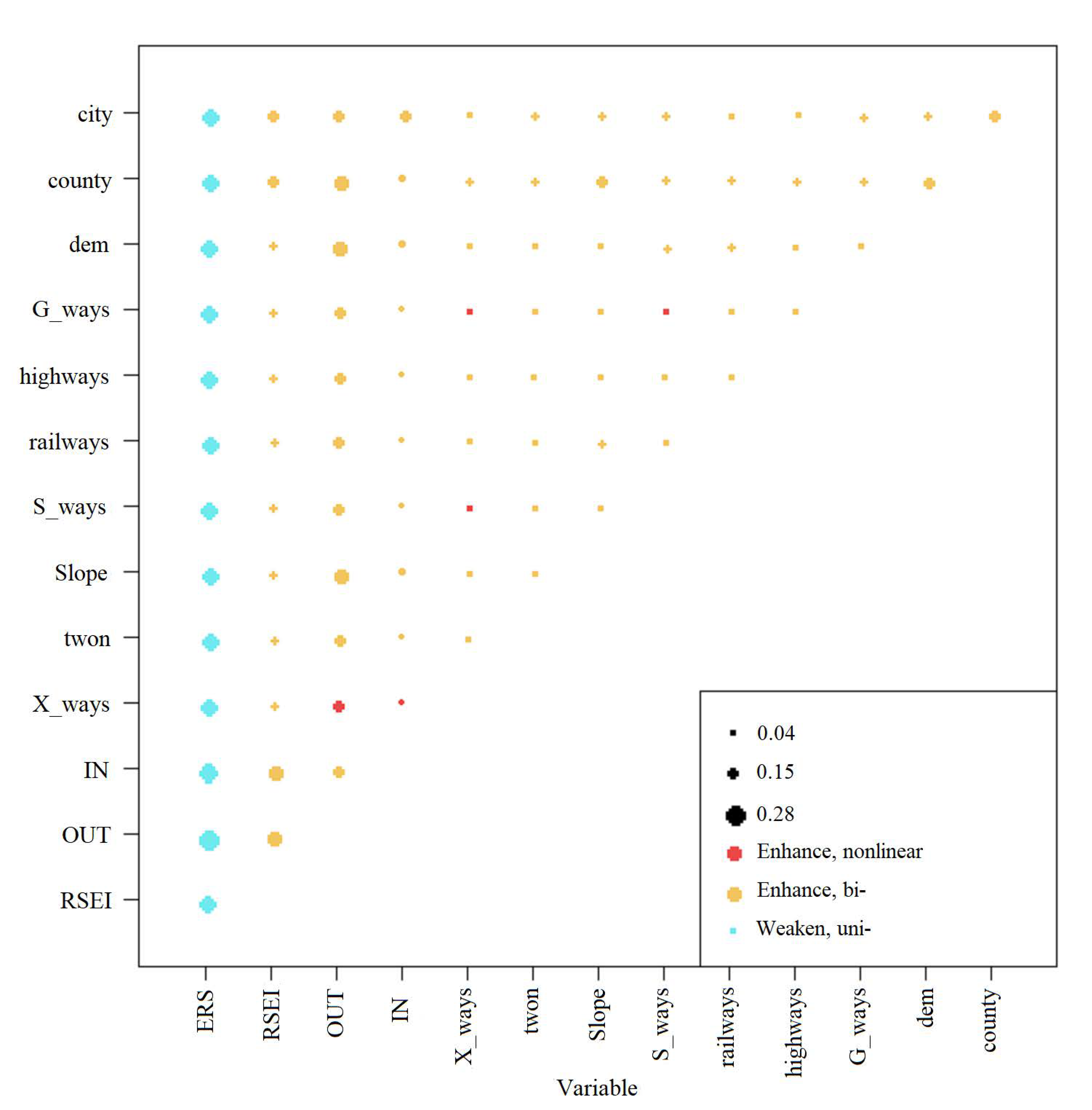
As shown in Table 7, the order of the top six spatial variables driving the urban expansion simulation is as follows: ERS (ecological resistance surface to urban expansion) > IN (urban inflow gravitational field) > OUT (urban outflow gravitational field) > county (distance from district and county centers) > RSEI (remote sensing ecological index) > city (distance from the city center). It can be seen that ecological constraints and the strength of the interaction force field between cities have a strong influence on urban land use change, followed by the distance from the district, county, and city centers. The dynamics of urban land use in Henan Province are the result of a combination of factors. The interaction of the drivers on urban land dynamics (Figure 8) shows bivariable enhancement and nonlinear enhancement, except for the interaction of ERS with other factors, which shows a univariable weakening effect. This indicates that ERS is the dominant factor among the factors, and when interacting with other factors, the effect of ERS is weakened.

5. Discussion

The factors influencing urban land use change are diverse and influenced by intercity interactions, the ecological environment, and local urban drivers. This study has implications for planning urban agglomerations in a macro sense and for the sustainable development of reconciling urban expansion with ecological conservation.
Currently, most studies examine cities as individuals, while urban development is not geographically or functionally isolated by local administrative boundaries [59]. The expansion of urban land in a city is greatly affected, not only by local driving forces, but also by intercity factors such as the distant influences of neighboring cities, especially the surrounding regional core cities in metropolitan areas [60]. In addition, some scholars have focused on the impact of ecology on urban expansion. However, most have considered only one focal region or city as the object of study [6,7,8,9,32,33], and there are few large-scale studies on the correlation between urban expansion and ecology. This study combines intercity interactions and the ecological environment for urban expansion research, which has vital practical and research significance.
Previous studies have indicated that the ecological environment and the strength of the urban gravity field are the two most significant factors influencing the expansion of urban agglomerations [28]. The simulation results of this study also demonstrate an improvement in the accuracy of simulating urban agglomerations. However, we observed a decrease in simulation accuracy when incorporating the urban spatial field strength factor after coupling it with ecological constraints. This decrease can be attributed to two factors. Firstly, the urban spatial field strength has been shown to enhance the accuracy of simulating developed cities [28], as these cities tend to have higher levels of urbanization and stronger urban spatial field intensities, attracting most resources to their vicinity, thereby exerting a stronger driving force on urban expansion. Secondly, the local ecological environment also plays a role. Ecologically rich areas require greater consideration for conservation needs, imposing constraints on urban expansion. The significant “potential difference” between ecological constraints and inter-city gravitational drivers allows ecological factors to dominate, thus diminishing the simulation accuracy.
This study explored the driving mechanisms of various factors using the OPGD model so that a more intuitive understanding of the influencing mechanisms of factors associated with the urban expansion can guide solving the problems existing policies and related factors may face. The analysis of factor-driven mechanisms of urban expansion indicated that intercity mobility significantly affects urban growth, as shown in previous studies [41,61].
The urban mobility data used in this study are a combination of population movement, search activity, and transportation connections, which reflect not only population interactions between cities, but also travel intentions and transportation connection conditions. In addition, urban expansion is a complex process, and the urbanization process generally destroys the ecological environment. This study uses RSEI and ERS to represent ecological quality factors, the former reflects the ecological quality status of the region [33] and the latter can reflect the spatial movement trend of urban expansion under ecological constraints [9]. From a macro perspective, urban growth is positively influenced by urban mobility, greater than the impact of ecological factors (RSEI) and other factors. Ecological constraints also have a significant impact on urban expansion. From a micro perspective, urban inflow is a stronger driver of urban expansion than the outflow of cities because urban inflow represents a city that is more attractive to other cities and, therefore, has more development opportunities. The driving effects of the ecological constraint factors, ERS and RSEI, ranked first and fifth, respectively, with ERS playing the strongest role. From the perspective of two-factor interaction, except for the weakening effect when ERS interact with other factors, all other two-factor interactions are enhanced, indicating that ERS is dominant in the urban expansion drive, which also indirectly explains why simulation accuracy decreases after the introduction of urban mobility factors in ecologically rich areas. The research results show that the urban gravitational field and ecological constraints have an important influence on urban expansion, which jointly affects cities’ scale and expansion direction and needs to be considered in urban planning and management. At the same time, the research results also provide a theoretical and practical basis for sustainable urban development and have certain reference values for formulating relevant policies and plans. According to the conclusion that urban interactions and ecological constraints jointly influence urban expansion, each region should consider local conditions and check and balance between socioeconomic development and the ecological environment, especially in areas with rapid urban development and a complex ecological environment. Rigid constraints can be applied to control urban expansion in important food-producing areas or areas with fragile ecologies, thereby achieving harmonious urbanization and ecological protection.
This study simulates urban land expansion in Henan Province by proposing a new framework for land use simulation with a coupled gravitational field model and ecological constraints and explores the effects of different factors on urban expansion. This may be useful for urban development and planning; however, some shortcomings exist. First, the expansion of urban agglomerations was influenced by policies in addition to topography, economy, and ecology. Policy data were not included in our experimental design due to a lack of data availability. Second, for the models adopted in this study, the urban flows in the micro-driving force analysis were derived from the calculated results based on the gravity model, which were different from the actual flow data and might have led to biased results. This study idealized urban spatial field strength, used constant values for the parameters, and ignored the influence of spatial and temporal disparities [62,63]. However, many scholars have adopted this calculation method because reasonable fixed parameters can reflect the overall field intensities of different cities [64]. In addition, this study uses the coupled gravitational field model and ecologically constrained land use model to simulate and predict urban use changes in Henan Province in 2020 and 2030. However, this does not mean that the model is applicable to other regions, and comparing the absolute contributions of the spatial interaction among inter-cities, ecological constraints, and other factors on urban expansion requires additional empirical and historical data to design a highly accurate model. The urban expansion simulation should be based on the actual ecological environment and social background and should be carried out to ensure the practicability of urban expansion [65] through the construction of social, ecological, economic, and other multi-indicators and multi-dimensional analysis. In future studies, to gain a more comprehensive and in-depth understanding, we propose the application of more detailed data to enable a more detailed examination. For example, multi-source heterogeneous spatial data can be fused to rationalize policies meticulously into urban simulation models to build more accurate models that reproduce the urban expansion modeling process.

6. Conclusions

This study constructed a new framework for land-use simulation with a coupled gravitational field model and ecological constraints from the perspective of urban interactions and the ecological environment. The experiment was conducted in Henan Province, China, to verify the feasibility of the method and to use the OPGD model to reveal the driving mechanism of urban land use change in the spatiotemporal pattern of Henan Province. The main conclusions are as follows:
(1) The proposed method can improve simulation accuracy at the scale of cities and urban agglomerations, particularly for the central cities of urban agglomerations (e.g., Zhengzhou);
(2) For local areas, the simulation results of the method are different when the gravitational field model and ecological constraints are coupled; the simulation results are better for urban developed areas after coupling the gravitational field model, and the simulation results are better for ecologically developed areas after coupling ecological constraints. Therefore, for cities with smaller scales and rich ecological resources, the simulation effect may be better if only a single factor of coupling ecological constraints is considered;
(3) The prediction of urban expansion in Henan Province in 2030 shows that inter-urban interaction forces and ecological condition constraints incorporated into urban expansion simulations can be better coordinated. The urban land use in Henan Province will increase from 2010 to 2030, and the urban land demand in Henan Province will reach 28,268.83 km2 by 2030;
(4) Through the analysis of the driving mechanism of urban land expansion, it was found that the intensity of urban spatial intensity and ecological constraints are two important factors affecting the expansion of urban agglomeration: urban interaction has a promoting effect on urban expansion, while the need for ecological protection has a restraining effect on urban expansion, and both work jointly to affect the expansion behavior of urban agglomeration.
To address the sustainable development issues of urban expansion and ecological protection, future urban development planning needs to consider both urban interactions and ecological environmental protection factors based on the actual socioeconomic and ecological environment and proactively take targeted measures to coordinate the relationship between urban, ecological, and sustainable development according to local conditions.

Author Contributions

Conceptualization, C.G.; methodology, C.G., Y.Z. and M.W.; validation, C.G., M.W. and Y.Z.; formal analysis, C.G., Y.Z. and M.W.; investigation, C.G.; resources, M.W. and Y.Z.; data curation, C.G.; writing—original draft preparation, C.G. and J.W.; writing—review and editing, C.G. and J.W.; visualization, C.G.; supervision, J.W.; All authors have read and agreed to the published version of the manuscript.

Funding

This research received no external funding.

Data Availability Statement

All data can be found in Section 3.2.

Acknowledgments

Acknowledgement for the data support from “National Tibetan Plateau Data Center (http://data.tpdc.ac.cn) (accessed on 9 September 2022)” and “National Earth System Science Data Center, National Science & Technology Infrastructure of China. (http://www.geodata.cn) (accessed on 9 September 2022)”.

Conflicts of Interest

The authors declare no conflict of interest.

References

  1. Fang, C.; Zhou, C.; Gu, C.; Chen, L.; Li, S. A proposal for the theoretical analysis of the interactive coupled effects between urbanization and the eco-environment in mega-urban agglomerations. J. Geogr. Sci. 2017, 27, 1431–1449. [Google Scholar] [CrossRef]
  2. Ye, Y.; Su, Y.; Zhang, H.-O.; Liu, K.; Wu, Q. Construction of an ecological resistance surface model and its application in urban expansion simulations. J. Geogr. Sci. 2015, 25, 211–224. [Google Scholar] [CrossRef]
  3. Zhang, M.; Kafy, A.-A.; Ren, B.; Zhang, Y.; Tan, S.; Li, J. Application of the Optimal Parameter Geographic Detector Model in the Identification of Influencing Factors of Ecological Quality in Guangzhou, China. Land 2022, 11, 1303. [Google Scholar] [CrossRef]
  4. Lopes, N.D.R.; Li, T.; Zhang, P.; Matomela, N.; Ikhumhen, H.O.; Sá, R.M. Predicting future coastal land use/cover change and associated sea-level impact on habitat quality in the Northwestern Coastline of Guinea-Bissau. J. Environ. Manag. 2022, 327, 116804. [Google Scholar] [CrossRef] [PubMed]
  5. Chang, D.; Li, S.; Lai, Z.; Fu, F.; Qi, X. Integrated effects of co-evolutions among climate, land use and vegetation growing dynamics to changes of runoff quantity and quality. J. Environ. Manag. 2023, 331, 117195. [Google Scholar] [CrossRef] [PubMed]
  6. Yang, X.; Bai, Y.; Che, L.; Qiao, F.; Xie, L. Incorporating ecological constraints into urban growth boundaries: A case study of ecologically fragile areas in the Upper Yellow River. Ecol. Indic. 2021, 124, 107436. [Google Scholar] [CrossRef]
  7. Ma, Q. Integrating ecological correlation into cellular automata for urban growth simulation: A case study of Hangzhou, China. Urban For. Urban Green. 2020, 51, 126697. [Google Scholar] [CrossRef]
  8. Cao, Y.; Zhang, X.; Fu, Y.; Lu, Z.; Shen, X. Urban spatial growth modeling using logistic regression and cellular automata: A case study of Hangzhou. Ecol. Indic. 2020, 113, 106200. [Google Scholar] [CrossRef]
  9. Yao, Y.; Ma, L.; Che, X.; Dou, H. Simulation study of urban expansion under ecological constraint—Taking Yuzhong County, China as an example. Urban For. Urban Green. 2021, 57, 126933. [Google Scholar] [CrossRef]
  10. Jiao, L.M.; Tang, X.; Liu, X.P. Spatial linkage and urban expansion: An urban agglomeration view. ISPRS-Int. Arch. Photogramm. Remote. Sens. Spat. Inf. Sci. 2017, XLII-2/W7, 1203–1211. [Google Scholar] [CrossRef] [Green Version]
  11. Cuiking, L.; Ying, L. Urban expansion simulation and analysis in the Beijing-Tianjin-Hebei Region. Prog. Geogr. 2015, 34, 217–228. [Google Scholar]
  12. Li, X.; Chen, Y.; Liu, X.; Li, D.; He, J. Concepts, methodologies, and tools of an integrated geographical simulation and optimization system. Int. J. Geogr. Inf. Sci. 2011, 25, 633–655. [Google Scholar] [CrossRef] [Green Version]
  13. Couclelis, H. Cellular Worlds: A Framework for Modeling Micro—Macro Dynamics. Environ. Plan. A 1985, 17, 585–596. [Google Scholar] [CrossRef]
  14. Verburg, P.H.; Soepboer, W.; Veldkamp, A.; Limpiada, R.; Espaldon, V.; Mastura, S.S.A. Modeling the Spatial Dynamics of Regional Land Use: The CLUE-S Model. Environ. Manag. 2002, 30, 391–405. [Google Scholar] [CrossRef]
  15. He, C.; Shi, P.; Chen, J.; Li, X.; Pan, Y.; Li, J.; Li, Y.; Li, J. Developing land use scenario dynamics model by the integration of system dynamics model and cellular automata model. Sci. China Ser. D Earth Sci. 2005, 48, 1979–1989. [Google Scholar] [CrossRef]
  16. Parker, D.C.; Manson, S.M.; Janssen, M.A.; Hoffmann, M.J.; Deadman, P. Multi-Agent Systems for the Simulation of Land-Use and Land-Cover Change: A Review. Ann. Assoc. Am. Geogr. 2003, 93, 314–337. [Google Scholar] [CrossRef] [Green Version]
  17. Santé, I.; García, A.M.; Miranda, D.; Crecente, R. Cellular automata models for the simulation of real-world urban processes: A review and analysis. Landsc. Urban Plan. 2010, 96, 108–122. [Google Scholar] [CrossRef]
  18. Aburas, M.M.; Ho, Y.M.; Ramli, M.F.; Ash’aari, Z.H. The simulation and prediction of spatio-temporal urban growth trends using cellular automata models: A review. Int. J. Appl. Earth Obs. Geoinf. 2016, 52, 380–389. [Google Scholar] [CrossRef]
  19. Castro, M.L.; Machado, P.; Santos, I.; Rodriguez-Fernandez, N.; Torrente-Patiño, A.; Carballal, A. State of the Art on Artificial Intelligence in Land Use Simulation. Complexity 2022, 2022, 2291508. [Google Scholar] [CrossRef]
  20. Qiang, Y.; Lam, N.S.N. Modeling land use and land cover changes in a vulnerable coastal region using artificial neural networks and cellular automata. Environ. Monit. Assess. 2015, 187, 57. [Google Scholar] [CrossRef] [PubMed]
  21. Feng, Y.; Liu, Y.; Batty, M. Modeling urban growth with GIS based cellular automata and least squares SVM rules: A case study in Qingpu–Songjiang area of Shanghai, China. Stoch. Environ. Res. Risk Assess. 2016, 30, 1387–1400. [Google Scholar] [CrossRef]
  22. Liu, Y.; Feng, Y.; Pontius, R.G. Spatially-Explicit Simulation of Urban Growth through Self-Adaptive Genetic Algorithm and Cellular Automata Modelling. Land 2014, 3, 719–738. [Google Scholar] [CrossRef] [Green Version]
  23. Liao, J.; Tang, L.; Shao, G.; Qiu, Q.; Wang, C.; Zheng, S.; Su, X. A neighbor decay cellular automata approach for simulating urban expansion based on particle swarm intelligence. Int. J. Geogr. Inf. Sci. 2014, 28, 720–738. [Google Scholar] [CrossRef]
  24. Liu, X.; Liang, X.; Li, X.; Xu, X.; Ou, J.; Chen, Y.; Li, S.; Wang, S.; Pei, F. A future land use simulation model (FLUS) for simulating multiple land use scenarios by coupling human and natural effects. Landsc. Urban Plan. 2017, 168, 94–116. [Google Scholar] [CrossRef]
  25. Lin, J.; He, P.; Yang, L.; He, X.; Lu, S.; Liu, D. Predicting future urban waterlogging-prone areas by coupling the maximum entropy and FLUS model. Sustain. Cities Soc. 2022, 80, 103812. [Google Scholar] [CrossRef]
  26. Gu, C.; Hu, L.; Zhang, X.; Wang, X.; Guo, J. Climate change and urbanization in the Yangtze River Delta. Habitat Int. 2011, 35, 544–552. [Google Scholar] [CrossRef]
  27. Limtanakool, N.; Schwanen, T.; Dijst, M. Ranking functional urban regions: A comparison of interaction and node attribute data. Cities 2007, 24, 26–42. [Google Scholar] [CrossRef]
  28. Lv, J.; Wang, Y.; Liang, X.; Yao, Y.; Ma, T.; Guan, Q. Simulating urban expansion by incorporating an integrated gravitational field model into a demand-driven random forest-cellular automata model. Cities 2021, 109, 103044. [Google Scholar] [CrossRef]
  29. Derudder, B.; Taylor, P. The cliquishness of world cities. Glob. Networks 2005, 5, 71–91. [Google Scholar] [CrossRef]
  30. Cao, H.; Wang, S. Analysis on the intensity of urban flow in the urban compact area of east Heilongjiang. Hum. Geogr. 2007, 22, 81–86. [Google Scholar]
  31. Yu, D.; Yanxu, L.; Bojie, F. Urban growth simulation guided by ecological constraints in Beijing city: Methods and implications for spatial planning. J. Environ. Manag. 2019, 243, 402–410. [Google Scholar] [CrossRef]
  32. Li, Y.; Ma, Q.; Song, Y.; Han, H. Bringing conservation priorities into urban growth simulation: An integrated model and applied case study of Hangzhou, China. Resour. Conserv. Recycl. 2019, 140, 324–337. [Google Scholar] [CrossRef]
  33. Han, N.; Hu, K.; Yu, M.; Jia, P.; Zhang, Y. Incorporating Ecological Constraints into the Simulations of Tropical Urban Growth Boundaries: A Case Study of Sanya City on Hainan Island, China. Appl. Sci. 2022, 12, 6409. [Google Scholar] [CrossRef]
  34. He, C.; Zhao, Y.; Tian, J.; Shi, P. Modeling the urban landscape dynamics in a megalopolitan cluster area by incorporating a gravitational field model with cellular automata. Landsc. Urban Plan. 2013, 113, 78–89. [Google Scholar] [CrossRef]
  35. Chuanglin, F. Progress and the future direction of research into urban agglomeration in China. Acta Geogr. Sin. 2014, 69, 1130–1144. [Google Scholar]
  36. Tian, G.; Qiao, Z.; Zhang, Y. The investigation of relationship between rural settlement density, size, spatial distribution and its geophysical parameters of China using Landsat TM images. Ecol. Model. 2012, 231, 25–36. [Google Scholar] [CrossRef]
  37. Poelmans, L.; Van Rompaey, A. Detecting and modelling spatial patterns of urban sprawl in highly fragmented areas: A case study in the Flanders–Brussels region. Landsc. Urban Plan. 2009, 93, 10–19. [Google Scholar] [CrossRef]
  38. You, H.; Yang, X. Urban expansion in 30 megacities of China: Categorizing the driving force profiles to inform the urbanization policy. Land Use Policy 2017, 68, 531–551. [Google Scholar] [CrossRef]
  39. Colantoni, A.; Grigoriadis, E.; Sateriano, A.; Venanzoni, G.; Salvati, L. Cities as selective land predators? A lesson on urban growth, deregulated planning and sprawl containment. Sci. Total Environ. 2016, 545–546, 329–339. [Google Scholar] [CrossRef] [PubMed]
  40. Tong, L.; Hu, S.; Frazier, A.E.; Liu, Y. Multi-order urban development model and sprawl patterns: An analysis in China, 2000–2010. Landsc. Urban Plan. 2017, 167, 386–398. [Google Scholar] [CrossRef]
  41. Lin, J.; Li, X. Simulating urban growth in a metropolitan area based on weighted urban flows by using web search engine. Int. J. Geogr. Inf. Sci. 2015, 29, 1721–1736. [Google Scholar] [CrossRef]
  42. James, P.E.; Martin, G.J. History of Geographical Thought; Xudan, L., Ed.; The Commercial Press: Beijing, China, 1989; pp. 481–482. [Google Scholar]
  43. Peng, G.; Ruihua, X. The Relationship between Urban Rail Transit and Urban Development Based on Gravitation Field Model. Syst. Eng. 2006, 1, 36–40. [Google Scholar]
  44. He, J.; Li, C.; Yu, Y.; Liu, Y.; Huang, J. Measuring urban spatial interaction in Wuhan Urban Agglomeration, Central China: A spatially explicit approach. Sustain. Cities Soc. 2017, 32, 569–583. [Google Scholar] [CrossRef]
  45. Hanqiu, X. A remote sensing urban ecological index and its application. Acta Ecol. Sin. 2013, 33, 7853–7862. [Google Scholar]
  46. Liping, H.; Ji, J. Remote Sensing Dynamic Monitoring on Temporal and Spatial Changes of Vegetation Coverage in Sichuan Province from 2009 to 2020. Bull. Soil Water Conserv. 2022, 42, 203–209. [Google Scholar]
  47. Liang, X.; Liu, X.; Li, X.; Chen, Y.; Tian, H.; Yao, Y. Delineating multi-scenario urban growth boundaries with a CA-based FLUS model and morphological method. Landsc. Urban Plan. 2018, 177, 47–63. [Google Scholar] [CrossRef]
  48. Baosheng, W.; Jiangfu, L.; Wei, Z.; Lin, Q.Q.W.; Lina, T. The weight of neighborhood setting of the FLUS model based on a historical scenario: A case study of land use simulation of urban agglomeration of the Golden Triangle of Southern Fujian in 2030. Acta Ecol. Sin. 2019, 39, 4284–4298. [Google Scholar]
  49. Jinfeng, W.; Chengdong, X. Geodetector: Principle and prospective. Acta Geogr. Sin. 2017, 72, 116–134. [Google Scholar]
  50. Peng, W.; Fan, Z.; Duan, J.; Gao, W.; Wang, R.; Liu, N.; Li, Y.; Hua, S. Assessment of interactions between influencing factors on city shrinkage based on geographical detector: A case study in Kitakyushu, Japan. Cities 2022, 131, 103958. [Google Scholar] [CrossRef]
  51. Huang, H.; Zhou, Y.; Qian, M.; Zeng, Z. Land Use Transition and Driving Forces in Chinese Loess Plateau: A Case Study from Pu County, Shanxi Province. Land 2021, 10, 67. [Google Scholar] [CrossRef]
  52. Tong, Z.; Jialin, W. On Driving Mechanism of Urban Expansion Based on Multi-source Nighttime Light Data: A Case Study of Three Urban Agglomerations in the Yangtze River Economic Belt. Sci. Technol. Manag. Land Resour. 2022, 39, 24–35. [Google Scholar]
  53. Song, Y.; Wang, J.; Ge, Y.; Xu, C. An optimal parameters-based geographical detector model enhances geographic characteristics of explanatory variables for spatial heterogeneity analysis: Cases with different types of spatial data. GISci. Remote Sens. 2020, 57, 593–610. [Google Scholar] [CrossRef]
  54. Peng, W.; Kuang, T.; Tao, S. Quantifying influences of natural factors on vegetation NDVI changes based on geographical detector in Sichuan, western China. J. Clean. Prod. 2019, 233, 353–367. [Google Scholar] [CrossRef]
  55. Wang, J.-F.; Zhang, T.-L.; Fu, B.-J. A measure of spatial stratified heterogeneity. Ecol. Indic. 2016, 67, 250–256. [Google Scholar] [CrossRef]
  56. Miaomiao, Y.; Qinke, Y.; Keli, Z.; Yuru, L.; Chunmei, W.; Guowei, P. Effects of Content of Soil Rock Fragments on Calculating of Soil Erodibility. Acta Pedol. Sin. 2021, 58, 1157–1168. [Google Scholar]
  57. Yang, Q. Soil Erodibility Dataset of Pan-Third Pole 20 countries (2020, with a resolution of 7.5 arc second). Natl. Tibet. Plateau Data Cent. 2021, 58, 1157–1167. [Google Scholar] [CrossRef]
  58. Peng, S.; Ding, Y.; Liu, W.; Li, Z. 1 km monthly temperature and precipitation dataset for China from 1901 to 2017. Earth Syst. Sci. Data 2019, 11, 1931–1946. [Google Scholar] [CrossRef] [Green Version]
  59. McHale, M.R.; Pickett, S.T.; Barbosa, O.; Bunn, D.N.; Cadenasso, M.L.; Childers, D.L.; Gartin, M.; Hess, G.R.; Iwaniec, D.M.; McPhearson, T.; et al. The New Global Urban Realm: Complex, Connected, Diffuse, and Diverse Social-Ecological Systems. Sustainability 2015, 7, 5211–5240. [Google Scholar] [CrossRef] [Green Version]
  60. Xia, C.; Zhang, A.; Wang, H.; Zhang, B.; Zhang, Y. Bidirectional urban flows in rapidly urbanizing metropolitan areas and their macro and micro impacts on urban growth: A case study of the Yangtze River middle reaches megalopolis, China. Land Use Policy 2018, 82, 158–168. [Google Scholar] [CrossRef]
  61. Tan, R.; Zhou, K.; He, Q.; Xu, H. Analyzing the Effects of Spatial Interaction among City Clusters on Urban Growth—Case of Wuhan Urban Agglomeration. Sustainability 2016, 8, 759. [Google Scholar] [CrossRef] [Green Version]
  62. Dock, J.P.; Song, W.; Lu, J. Evaluation of dine-in restaurant location and competitiveness: Applications of gravity modeling in Jefferson County, Kentucky. Appl. Geogr. 2015, 60, 204–209. [Google Scholar] [CrossRef]
  63. Natale, F.; Borrello, A.; Motova, A. Analysis of the determinants of international seafood trade using a gravity model. Mar. Policy 2015, 60, 98–106. [Google Scholar] [CrossRef]
  64. Xia, C.; Zhang, A.; Wang, H.; Zhang, B. Modeling urban growth in a metropolitan area based on bidirectional flows, an improved gravitational field model, and partitioned cellular automata. Int. J. Geogr. Inf. Sci. 2019, 33, 877–899. [Google Scholar] [CrossRef]
  65. Huang, A.; Xu, Y.; Liu, C.; Lu, L.; Zhang, Y.; Sun, P.; Zhou, G.; Du, T.; Xiang, Y. Simulated town expansion under ecological constraints: A case study of Zhangbei County, Heibei Province, China. Habitat Int. 2019, 91, 101986. [Google Scholar] [CrossRef]
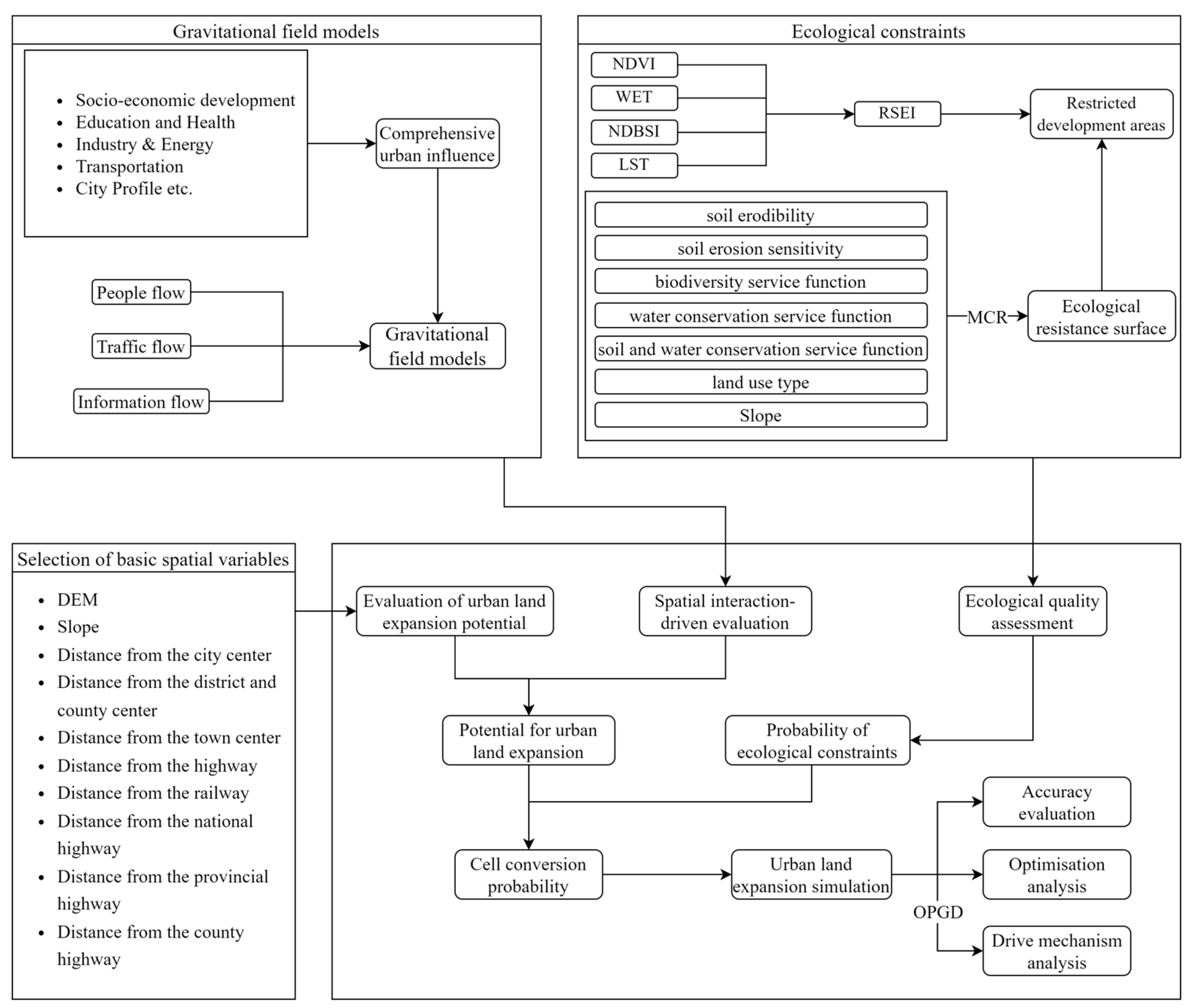
Figure 1. Flow chart of the research framework.
Land 12 01189 g001
Figure 2. Map of the study area of Henan Province.
Land 12 01189 g002
Figure 3. Underlying spatial variables related to urban land expansion. DEM, DEM; Slope, slope; city, distance from the city center; County, distance from the district and county center; town, distance from the town center; highways, distance from the highway; railways, distance from the railway; G_ways, distance from the national highway; S_ways, distance from the provincial highway; X_ways, distance from the county highway.
Land 12 01189 g003
Figure 4. Distribution of total inflows, total outflows, influence, and linkage intensity by city and gravitational field strength between cities in the study area.
Land 12 01189 g004
Figure 5. Map of the distribution of the factors and restricted areas of the ecological assessment. K represents soil erodibility; Si, soil erosion sensitivity; Sbio, biodiversity service function; WR, water retention service function; Spro, soil and water conservation service function; Type, land use type; Slope, slope; and ERS, ecological resistance surface.
Land 12 01189 g005
Figure 6. (A) The 2010–2020 simulation results for different coupling scenarios and (B) regional accuracy for different coupling scenarios.
Land 12 01189 g006aLand 12 01189 g006b
Figure 7. Graph of urban expansion projection results for 2020–2030 with a coupled gravitational field model and ecological constraints.
Land 12 01189 g007
Figure 8. Interaction of the drivers with the dynamics of urban land use.
Land 12 01189 g008
Table 1. Integrated City Impact Indicator System.
City Impact Evaluation Indicator SystemIndicators
Socioeconomic developmentTotal GDP (X1), total retail sales of consumer goods (X2), average employee wages (X3), population (X4)
Education and HealthNumber of students enrolled in higher education (X5), number of health institutions (X6), number of higher education institutions (X7)
Industry and EnergyNumber of industrial enterprise units above scale (X8), electricity consumption of the entire society (X9)
TransportationPassenger transport volume (X10), freight transport volume (X11), total post and telecommunications services (X12)
City overviewArea of built-up urban areas (X13), parkland area per capita (X14), greening coverage of built-up areas (X15)
Table 2. Resistance levels of the resistance factor, and values of the resistance of urban expansion ecology.
Value of Ecological Resistance to Urban ExpansionType of Land UseSlope (Degree)
1Urban building land0–3
3Bare land, facility land3–8
5Arable land, grassland8–15
7Woodland15–25
9Water areas, nature reserves>25
Table 3. Conversion cost matrix.
Cultivated LandForestGrasslandShrublandWetlandWater BodyArtificial SurfacesBare Land
Cultivated Land11010010
Forest11110001
Grass Land10100011
Shrubland11110001
Wetland10101111
Water Body10101111
Artificial Surfaces00000010
Bare Land11111111
Table 4. Information and sources of data used in this study.
DataTypeResolutionSource
Basic dataBasic geospatial data (including administrative areas, urban points, roads, etc.)VectorNational Geomatics Centre of China (http://www.ngcc.cn/ngcc/) (accessed on 24 August 2022)
Land use dataRaster30 mGlobeLand30
(http://www.globallandcover.com/)(accessed on 24 August 2022)
DEMRaster30 mGeospatial Data Cloud (http://www.gscloud.cn/search) (accessed on 24 August 2022)
Gravitational field model dataCity Impact Evaluation IndicatorsPropertiesyearHenan Statistical Yearbook 2020
Baidu Index DataProperties1 January 2020–31 December 2020Baidu Index official website (https://index.baidu.com/v2/index.html#/)
Traffic Flow DataPropertieshttp://www.114piaowu.com, 12306 China railway (accessed on 3 September 2022)
Population migration dataProperties1 January 2020–31 December 2020AutoNavi Maps Traffic Big Data (https://trp.autonavi.com/home.html) (accessed on 3 September 2022)
Ecological constraints dataRESI (NDVI, WET, NDBSI, LST)Raster30 mLandsat-8 (obtained from Google Earth Engine platform processing)
Soil erodibility (K) [56,57]Raster7.5 arc sNational Tibetan Plateau Data Center (http://data.tpdc.ac.cn) (accessed on 9 September 2022)
Rainfall data and temperature data [58]Raster1 km National Earth System Science Data Center, National Science & Technology Infrastructure of China. (http://www.geodata.cn) (accessed on 9 September 2022)
Average annual net primary productivity of vegetationRaster500 mNational Aeronautics and Space Administration (https://ladsweb.modaps.eosdis.nasa.gov/search/) (accessed on 9 September 2022)
Soil infiltration factor dataRaster1 kmGlobal Soil Database
Table 5. Weighting values of factors for each land use type.
Cultivated LandForestGrasslandShrublandWetlandWater BodyArtificial SurfacesBareland
Weight0.50.710.750.740.760.761.00.75
Table 6. Accuracy verification results for different coupling scenarios.
Kappa CoefficientOverall AccuracyFOM
A0.7235290.8446120.068728
B0.7241080.8451810.071257
C0.7301330.8485360.082824
D0.7308440.8486760.083005
Table 7. Q-statistic values for each factor of the factor detection results.
Q-Statistic
ERS0.5064 **
IN0.152 **
OUT0.1495 **
county0.1148 **
RSEI0.0992 **
city0.0735 **
Slope0.0678 **
dem0.0661 **
railways0.0593 **
S_ways0.0489 **
G_ways0.0469 **
highways0.0338 **
town0.0332 **
X_ways0.0104 **
** represents Q values significant at the 0.001 level (p < 0.001).
Disclaimer/Publisher’s Note: The statements, opinions and data contained in all publications are solely those of the individual author(s) and contributor(s) and not of MDPI and/or the editor(s). MDPI and/or the editor(s) disclaim responsibility for any injury to people or property resulting from any ideas, methods, instructions or products referred to in the content.