Optimization of Green Spaces in Plain Urban Areas to Enhance Carbon Sequestration

Abstract

Global climate change and rapid urbanization have placed enormous pressure on the urban ecological environment worldwide. Urban green spaces, which are an important component of urban ecosystems, can maintain ecological and environmental sustainability and benefits, including biodiversity conservation and carbon sequestration. However, land use changes across urban landscapes, especially in plain urban areas with high development pressure, have significantly impacted the carbon sequestration efficiency of urban green spaces. Nevertheless, research examining the impact of land use change and development pressure on urban green spaces and carbon sequestration is relatively scarce. Understanding the carbon sequestration efficiency of urban green spaces and its determining factors will help predict future carbon capture trends within urban ecosystems and formulate more targeted sustainable urban planning and management strategies to improve urban carbon sink efficiency and achieve the goal of carbon neutrality. Therefore, to understand the factors affecting the carbon sequestration efficiency of urban green spaces, this paper used an integrated framework that combined the Carnegie–Ames–Stanford approach (CASA) model, landscape pattern index, multiple linear regression, and Markov–FLUS model. The study explored the impact of urban land use and land cover changes on carbon sequestration within the plain urban areas of Beijing at street scale. The results showed that, at street scale, there was a significant positive and negative correlation between the landscape pattern index and net primary productivity (NPP). In addition, the green spaces located in areas with more complex landscape structures had better carbon sequestration benefits. In addition, multiscenario carbon sequestration efficiency prediction suggested that the sustainable development (SD) scenario could achieve a positive increment of overall NPP. In contrast, the business-as-usual development (BD), the fast development (FD), and the low development (LD) scenarios showed a downward trend in NPP. This paper also proposed strategies for optimizing and enhancing green spaces within urban plain areas. Based on the strategies, the results guide decision making for sustainable urban green space planning that maintains the ecological, economic, and social integrity of urban landscapes during urbanization.

1. Introduction

As one of the megacities in China, Beijing has experienced significant land use and land cover changes during the last few decades, severely compromising the services provided by urban ecosystems, particularly urban green spaces. For instance, urban expansion in the Beijing–Tianjin–Hebei region from 1988 to 2008 led to a significant decline in cultivated land and associated ecosystem services, such as freshwater, nutrient cycling, soil conservation, and organic production [1,2,3,4]. In addition, urbanization in the Beijing–Tianjin–Hebei region from 2005 to 2015 has led to a decrease in NPP [5]. However, in recent years, China has proposed goals to conserve natural resources in and around urban landscapes and achieve carbon neutrality by 2050. Especially, increased attention to research and development has been given to identifying various ways for increasing ecosystem services, including the ecosystem carbon sequestration and storage capacity, to achieve the proposed goal of carbon neutrality by 2050 [6].

Net primary productivity (NPP), the ability of vegetation to sequester carbon per unit area and per unit time, also expressed as the portion of organic carbon captured during photosynthesis minus utilized by respiration, can be used as a surrogate measurement of vegetation carbon sequestration capacity [7]. Because NPP strongly correlates with vegetation carbon sink capacity, similar factors may govern the spatial and temporal patterns of NPP and vegetation carbon sink capacity [8]. Several previous studies have used NPP as a surrogate to measure the carbon sequestration capacity of vegetation [5,9,10]; this paper also uses NPP to represent the carbon sequestration capacity of urban vegetation.

Previous studies evaluated the effects of land use and land cover change in NPP and, thus, carbon sequestration across various ecosystems [11,12]. For instance, scholars explore the loss of NPP due to urban expansion in Guangdong Province, China [13,14]. Similarly, other scholars evaluated the impact of land use change on NPP from urban vegetation in Guangzhou, China, finding that the conversion of grassland and forestland into construction land caused a decline in the NPP of grasslands and forests [15]. The landscape pattern indices, which reflect the structure and spatial layout of regional green spaces, have typically been used to analyze the spatiotemporal changes in green spaces and identify the relationship between landscape patterns and NPP [16]. For example, Asplund analyzed the impact of landscape pattern changes on the regional carbon sequestration capacity of the mangrove–seagrass coastal bays in northwestern Madagascar [17]. Furthermore, scholars analyzed the relationship between NPP and landscape patterns using landscape pattern indices in the Shule River Basin [18].

Existing research demonstrating the relationship between NPP, land use change, and landscape pattern change has mostly been focused on larger geographical areas, such as cities, regions, and provinces [16]. However, there is limited research covering microregions (e.g., blocks and streets) of the urban landscape. To address this research gap, this paper aims to evaluate the relationships between NPP and land use and landscape pattern change at street scale within the urban plain areas in Beijing, China. This research also evaluated the relationship between NPP and historical and contemporary land use and landscape pattern changes. Understanding the relationships between NPP and land use and landscape pattern changes at street scale may help to initiate the multilevel coordinated efforts, from private companies and government agencies, for reducing carbon emissions and achieving the goal of carbon neutrality. Because little is known about how future land use and landscape pattern changes will drive NPP [19,20], this study also evaluated the effect of potential future changes in land use and landscape patterns on NPP. Predicting the status of NPP under future changes in land use and landscape patterns in the rapidly developing urban plain areas of Beijing will help formulate effective green space management strategies and achieve carbon neutrality.

The key to analyzing the future changes in NPP under different scenarios is to accurately simulate the spatiotemporal changes in future land use by using different development scenarios [21]. The Future Land Use Simulation (FLUS) model is a commonly used method for predicting land use changes [22]. For instance, Xiang used the Markov–FLUS model to predict the land use patterns in the main urban areas within Chongqing for 2035 under four scenarios [23]. They also analyzed the relationship between the future regional carbon sequestration capacity of green spaces and land use changes. The FLUS model was also used to predict the land use changes in the Loess Plateau under three scenarios and simulate and analyze the changes in NPP under multiple scenarios [24]. These studies show that the FLUS model has high prediction accuracy and can reasonably predict and analyze the effects of future land use change on NPP.

This study combined these research methods and established a high-precision multiple linear regression model to predict future changes in NPP based on the correlation between spatiotemporal changes in NPP and landscape patterns. The Markov–FLUS model was used to predict future changes in land use and landscape pattern indices and quantify the landscape patterns of green spaces under different scenarios. This study investigated the impact of spatiotemporal changes in green space landscape patterns on regional carbon sink performance. The specific goals were to (1) quantify the spatiotemporal relationships between the NPP and landscape patterns of green spaces; (2) determine the impact of changes in landscape patterns of urban green spaces on NPP; and (3) propose strategies for optimizing the spatial patterns of green space in plain areas of megacities. Results from this study provide scientific evidence for optimizing land use configuration and improving the landscape patterns of green spaces at a regional level. In addition, this study provides some guidelines for enhancing ecosystem services, optimizing the green space landscape patterns in the plain areas of megacities, and promoting regional low-carbon development.

2. Materials and Methods

2.1. Research Object

Beijing, the capital city of China, is one of the most populous cities in the world. The city occupies approximately 16,410 km² and is situated at the meeting point of the Taihang Mountains, Yanshan Mountains, and the northern China Plain. It is about 150 km from the Bohai Sea Gulf. The plain area of Beijing is primarily located in the southeast part of the city and comprises several highly developed areas, including Dongcheng, Xicheng, Chaoyang, Haidian, Fengtai, and Shijingshan (Figure 1). Plains and hills characterize the topography of the area, and the climate is mild, humid continental, with an average annual temperature of 10 °C. With a high degree of urbanization, such as advanced transportation, commerce, culture, and education facilities, the plain area of Beijing constitutes an important economic, cultural, and educational center. In recent years, however, the land use types and landscape patterns of the area, particularly the eastern side occupying 97.22% (6408 km²) of the total plain area, have constantly been changing. Because of its ecological, economic, cultural, and social significance, this study selected the east side of the plain area as the research object.

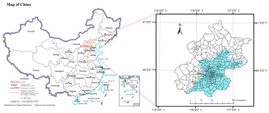
Figure 1. Map of the study area showing the extent of the plain area on the eastern side of Beijing.

2.2. Data Acquisition

All the data required for the study are listed in Table 1.

Table 1. Various data categories, types, units of measurement, and data sources used in the study.

Data Category	Data Type	Dots Per Inch (DPI)/m	Data Resources
Remote sensing	Remote sensing image of Beijing (1999, 2004, 2011, 2014, 2019)	30 m	Geospatial Data Cloud (http://www.gscloud.cn/ accessed on 28 February 2023)
Environmental	Land use data (1999, 2004, 2011, 2014, 2019)	30 m	Processed from remote sensing images
	DEM	30 m	Geospatial Data Cloud (http://www.gscloud.cn/ accessed on 28 February 2023)
	Aspect	30 m	Calculated from DEM
	Slope	30 m	Calculated from DEM
	NDVI	30 m	Processed from remote sensing images
	Annual/monthly average temperature	1000 m/30 m	GOEDATA (http://www.geodata.cn/ accessed on 28 February 2023)
	Annual average precipitation	1000 m
	Monthly total precipitation	30 m
	Monthly total radiation	10,000 m	TPDC (https://data.tpdc.ac.cn/ accessed on 28 February 2023)
	Distance to river	30 m	CAS (http://www.resdc.cn/ accessed on 28 February 2023)
Socioeconomic	Population	1000 m	CAS (http://www.resdc.cn/ accessed on 28 February 2023)
	GDP	1000 m
	Road network	Vector	Open street Map (http://www.openstreetmap.org/ accessed on 28 February 2023)
	Distance to expressway	30 m
	Distance to railway	30 m	Processed from road network
	Distance to railway station	30 m
	Distance to national highway	30 m
	Distance to primary road	30 m
	Distance to secondary road	30 m
	Distance to tertiary road	30 m
	Distance to POI	30 m	CAS (http://www.resdc.cn/ accessed on 28 February 2023)

2.2.1. Downloading and Preprocessing of Remote Sensing Images

Remote sensing satellite images of Beijing were obtained from the Geospatial Data Cloud (http://www.gscloud.cn/ accessed on 28 February 2023). The images from 1999, 2004, and 2011 were taken from Landsat 4 and 5, while images from 2014 and 2019 were taken from Landsat 8. A total of 10 image maps representing plain areas with a spatial resolution of 30 m × 30 m were selected. The original data were processed by cutting, stitching, radiometric calibration, and atmospheric correction to obtain preprocessed images. Using unsupervised classification, land use types for the urban green spaces were classified into built-up land, water bodies, grassland, woodland, cultivated land, and unused land.

2.2.2. Data Source for NPP Calculation

NPP was calculated by integrating vegetation cover, normalized difference vegetation Index (NDVI), and meteorological data, and using the CASA model. Vegetation cover data were obtained from the Earth Big Data Science Engineering Data Sharing Service System (https://data.casearth.cn/ accessed on 28 February 2023), and NDVI data were obtained from ENVI-processed remote sensing images. Meteorological data, monthly average temperature, and monthly total precipitation were obtained from the National Earth System Science Data Center (http://www.geodata.cn/ accessed on 28 February 2023). Monthly total radiation data were obtained from the National Tibetan Plateau Data Center (https://data.tpdc.ac.cn/ accessed on 28 February 2023). Meteorological data were processed in ArcGIS software using the geospatial interpolation techniques, kriging and raster sampling, with a spatial resolution of 30 m × 30 m.

2.2.3. Data Source for FLUS Prediction Model

The FLUS model was built using data from land use and the driving factors. The land use data were derived from the remote sensing satellite images. The driving factors are divided into natural environmental factors and socioeconomic factors. Natural environmental factors include slope, aspect, digital elevation model (DEM), NDVI, and meteorological factors. Slope, aspect, and the DEM (digital elevation model) with 30 m resolution were sourced from the Geographic Spatial Data Cloud Platform (gscloud.cn) and calculated in ArcMap 10.6. NDVI data were sourced from remote sensing images, and annual average temperature and precipitation data were sourced from the National Earth System Science Data Center (http://www.geodata.cn/ accessed on 28 February 2023). The gross domestic product (GDP), population density, and socioeconomic data were sourced from the Resource and Environmental Science and Data Center (https://www.resdc.cn/ accessed on 28 February 2023). Distances to railways, expressways, national roads, train stations, first-, second-, and third-level roads, and river systems were obtained by processing the traffic network of OpenStreet Map (http://www.openstreetmap.org/ accessed on 28 February 2023) with ArcGIS. Finally, restriction factors were obtained by reclassifying the land use data in ArcGIS.

2.3. Methods

This analysis uses the CASA and land use prediction models, landscape pattern index calculation, and correlation analysis. A schematic for the research methods used in the study is shown in Figure 2.

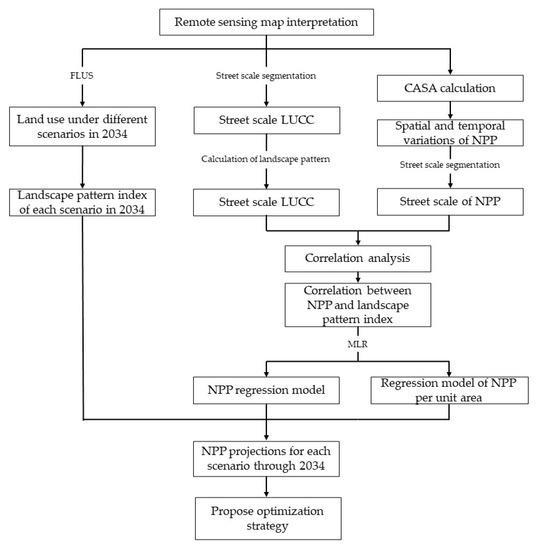
Figure 2. A schematic showing data acquisition and analyses to optimize strategies and technical approaches for green space in the plain areas of Beijing.

2.3.1. Carnegie–Ames–Stanford Approach (CASA) Model

This study used the improved CASA model [25], originally derived from the CASA model, to calculate NPP. The improved model overcomes the disadvantages of using the maximum light-use efficiency (εmax) for world vegetation as a constant value. The paper followed this approach to obtain the vegetation types and regional environmental variables in the Beijing area and determine εmax and NPP [26]:

$$\mathrm{NPP}\left(\mathrm{x},\mathrm{t}\right)=\mathrm{APAR}\left(\mathrm{x},\mathrm{t}\right)\times \mathsf{\epsilon }\left(\mathrm{x},\mathrm{t}\right)$$

where NPP(x,t) is the photosynthetically active radiation at a specific time and location, APAR(x,t) is the absorbed photosynthetically active radiation, and ε(x,t) is the actual light energy utilization efficiency of plants. Because of the size of the study area, the relationship between NPP and landscape pattern indices, together with carbon sink efficiency, were determined at street scale.

2.3.2. Landscape Pattern Indices Calculation

Landscape pattern analysis is an important method for quantitatively analyzing the relationships between spatiotemporal characteristics of landscape structure and spatial layout. The landscape pattern index can summarize the spatial information of the landscape in different dimensions and become an important indicator of its spatial distribution and structural characteristics [27]. Considering the effectiveness of landscape indices in quantifying changes in landscape patterns and analyzing their influence on NPP [28,29], this study selected 19 different indices representing area and edge, aggregation, density, diversity, and shape, following [30] (Table 2). In this study, the landscape indices were calculated at street scale to investigate indices relationships with NPP.

Table 2. Different types of landscape indices used in the study.

Grade	Type	Index	Explanation	Formula
Category	Area and Edge metrics	CA/TA	Sum of areas of corresponding plaque types	$\mathrm{CA}={\displaystyle \sum _{\mathrm{j}=1}^{\mathrm{n}}{{\displaystyle \mathrm{a}}}_{\mathrm{ij}}}\left(\frac{1}{\mathrm{10,000}}\right)$
	The magnitude and difference of density	NP	Number of patches within the landscape	$\mathrm{NP}=\mathrm{N}$
	The magnitude and difference of density	PD	The density of a certain patch in the landscape can reflect the overall heterogeneity and fragmentation of the landscape and the degree of fragmentation of a certain type, reflecting the heterogeneity of the landscape per unit area	$\mathrm{PD}=\frac{\mathrm{N}}{\mathrm{A}}\left(\mathrm{10,000}\right)\left(100\right)$
	Aggregation metrics	MESH	The ratio of the sum of squares of patch areas to the total landscape area can be used to compare the average patch area in the landscape; when the total area of the landscape remains unchanged, the effective grid becomes larger, reflecting the increase in the area of this type, indicating that its proportion in the landscape increases	$\mathrm{MESH}=\frac{{\displaystyle \sum _{\mathrm{j}=1}^{\mathrm{n}}{{\displaystyle {{{\displaystyle \mathrm{a}}}_{\mathrm{ij}}}^2}}_{}}}{\mathrm{A}}\left(\frac{1}{\mathrm{10,000}}\right)$
	Aggregation metrics	DIVISION	The landscape segmentation index reflects the separation degree of patches in the landscape, and the larger the value, the more fragmented the patch composition and the more complex the landscape	$\mathrm{DIVISION}=\left[1-{\displaystyle \sum _{\mathrm{j}=1}^{\mathrm{n}}{\left(\frac{{{\displaystyle \mathrm{a}}}_{\mathrm{ij}}}{\mathrm{A}}\right)}^2}\right]$
	Aggregation metrics	IJI	This refers to the overall distribution and juxtaposition among plaque types; a small value indicates that plaque type i is contiguous to only a few other types	$\mathrm{IJI}=\frac{-{\displaystyle \sum _{\mathrm{k}=1}^{\mathrm{m}}\left[{\mathrm{P}}_{\mathrm{i}}\left(\frac{{{\displaystyle \mathrm{g}}}_{\mathrm{ik}}}{{\displaystyle \sum _{\mathrm{k}=1}^{\mathrm{m}}{{\displaystyle \mathrm{g}}}_{\mathrm{ik}}}}\right)•\left[\ln \left(\frac{{{\displaystyle \mathrm{g}}}_{\mathrm{ik}}}{{\displaystyle \sum _{\mathrm{k}=1}^{\mathrm{m}}{{\displaystyle \mathrm{g}}}_{\mathrm{ik}}}}\right)\right]\right]}}{\ln \left(\mathrm{m}-1\right)}\left(100\right)$
	Aggregation metrics	SPIT	An increase in SPLIT represents a decrease in the area of major plaque types and subdivisions into smaller plaques	$\mathrm{SPLIT}=\frac{{\mathrm{A}}^2}{{\displaystyle \sum _{\mathrm{j}=1}^{\mathrm{n}}{{\displaystyle {\mathrm{a}}_{\mathrm{ij}}}}^2}}$
	Shape metrics	SHAPE-MN	The larger the value, the more complex the landscape patch shape	$\mathrm{SHAPE}-\mathrm{MN}=\frac{{0.25\mathrm{P}}_{\mathrm{ij}}}{\sqrt{{\mathrm{a}}_{\mathrm{ij}}}}$
	Area and Edge metrics	AREA-MN	Represents the average patch area	$\mathrm{AREA}-\mathrm{MN}={-\mathrm{a}}_{\mathrm{ij}}\left(\frac{1}{\mathrm{10,000}\mathrm{n}}\right)$
	Area and Edge metrics	PLAND	Patch area percentage, also known as patch area proportion, is the proportion of various types of land in the total area, and main landscape represents the largest area	$\mathrm{PLAND}={\mathrm{P}}_{\mathrm{i}}\frac{{\displaystyle \sum _{\mathrm{j}=1}^{\mathrm{n}}{{\displaystyle {{\displaystyle \mathrm{a}}}_{\mathrm{ij}}}}_{}}}{\mathrm{A}}\left(100\right)$
	Area and Edge metrics	LPI	Maximum patch percentage of landscape	$\mathrm{LPI}=\frac{\underset{\mathrm{j}=1}{\overset{}{\stackrel{\mathrm{a}}{\max }}}\left({\mathrm{a}}_{\mathrm{ij}}\right)}{\mathrm{A}}\left(100\right)$
	Area and Edge metrics	ED	This refers to the degree to which the landscape or type is divided by the boundary, which directly reflects the degree of landscape fragmentation; the higher the boundary density, the higher the landscape fragmentation	$\mathrm{ED}=\frac{{\displaystyle \sum _{\mathrm{k}=1}^{\mathrm{n}}{{\displaystyle {{\displaystyle \mathrm{e}}}_{\mathrm{ik}}}}_{}}}{\mathrm{A}}\left(\mathrm{10,000}\right)$
Landscape	Diversity metrics	SHEI	SHEI is equal to SHDI divided by the maximum possible diversity of a given landscape abundance (each block type is equally distributed); the smaller the SHEI value, the dominant patch type may dominate the landscape.	$\mathrm{SHEI}=\frac{-{\displaystyle \sum _{\mathrm{i}=1}^{\mathrm{m}}{{\displaystyle \left({\mathrm{P}}_{\mathrm{i}}\cdot {\mathrm{lnP}}_{\mathrm{i}}\right)}}^{}}}{\ln \mathrm{m}}$
	Aggregation metrics	CONTAG	This refers to the aggregation degree or extension trend of different patch types in the landscape; a high spread value indicates that some dominant types form good connectivity in the landscape, which indicates that the landscape is a dense pattern with multiple elements	$\mathrm{CONTAG}=\frac{-{\displaystyle \sum _{\mathrm{i}=1}^{\mathrm{m}}{\displaystyle \sum _{\mathrm{k}=1}^{\mathrm{m}}\left[{\mathrm{P}}_{\mathrm{i}}\left(\frac{{{\displaystyle \mathrm{g}}}_{\mathrm{ik}}}{{\displaystyle \sum _{\mathrm{k}=1}^{\mathrm{m}}{{\displaystyle \mathrm{g}}}_{\mathrm{ik}}}}\right)•\left[\ln \left(\mathrm{p}•\frac{{{\displaystyle \mathrm{g}}}_{\mathrm{ik}}}{{\displaystyle \sum _{\mathrm{k}=1}^{\mathrm{m}}{{\displaystyle \mathrm{g}}}_{\mathrm{ik}}}}\right)\right]\right]}}}{2\ln \left(\mathrm{m}\right)}\left(100\right)$
	Diversity metrics	SHDI	This reflects landscape heterogeneity and is more sensitive to the unbalanced distribution of patch types; in a landscape system, the richer land use, the higher the degree of fragmentation and the SHDI value	$\mathrm{SHDI}=-{\displaystyle \sum _{\mathrm{i}=1}^{\mathrm{m}}{{\displaystyle \left({\mathrm{P}}_{\mathrm{i}}\cdot {\mathrm{lnP}}_{\mathrm{i}}\right)}}^{}}$
	Aggregation metrics	ED	This refers to the degree in which the landscape or landscape type is divided by the boundary, directly reflecting the landscape fragmentation; the higher the boundary density, the higher the landscape fragmentation.	$\mathrm{ED}=\frac{{\displaystyle \sum _{\mathrm{k}=1}^{\mathrm{n}}{{\displaystyle {{\displaystyle \mathrm{e}}}_{\mathrm{ik}}}}_{}}}{\mathrm{A}}\left(\mathrm{10,000}\right)$
	Area and Edge metrics	CA/TA	Sum of areas of corresponding plaque types	$\mathrm{CA}={\displaystyle \sum _{\mathrm{j}=1}^{\mathrm{n}}{{\displaystyle \mathrm{a}}}_{\mathrm{ij}}}\left(\frac{1}{\mathrm{10,000}}\right)$
	The magnitude and difference of density	PRD	Represents the richness and density of a certain patch in the landscape	$\mathrm{PD}=\frac{\mathrm{m}}{\mathrm{A}}\left(\mathrm{10,000}\right)\left(100\right)$
	Area and Edge metrics	LPI	Maximum patch percentage of landscape	$\mathrm{LPI}=\frac{\underset{\mathrm{j}=1}{\overset{}{\stackrel{\mathrm{a}}{\max }}}\left({\mathrm{a}}_{\mathrm{ij}}\right)}{\mathrm{A}}\left(100\right)$

2.3.3. Statistical Analysis

This study calculated the Pearson correlation coefficient [31] between the monthly mean NPP for September 2019 and the landscape pattern indices at street scale. Two multiple linear regression (MLR) models of total NPP and landscape pattern indices and per unit area NPP and landscape pattern indices were developed following correlation coefficient results to predict future NPP. The models were validated using the September 2014 data (repeated 237 times at street scale). The coefficient of determination (R²) and root mean square error (RMSE) were calculated to quantify how well a model fit a data set [32]. A stepwise MLR method was chosen to reduce interference with the regression models because of the high correlation between different landscape indices. The adjusted R² indicated the predictive ability of the MLR model. The relative importance of landscape indices to NPP was measured using standardized coefficients (beta). SPSS software was used to select landscape indices highly correlated with NPP and established an objective MLR model at the landscape and type level. In the stepwise MLR analysis, models were selected by applying the following measures: (1) the highest adjusted R² value among all models, (2) the model coefficients and significance of the independent variables equal to or less than 0.001 (p ≤ 0.001), and (3) the variance inflation factor (VIF) of all predictor variables less than 10, ensuring that collinearity had no adverse effects on the models [30]. The MLR models were also used to predict NPP for 2034 in the subsequent land use prediction.

2.3.4. Scenario Setting

The study considered land use forecast development scenarios based on a comprehensive analysis of various land use scenarios, including representative concentration pathways and shared socioeconomic pathways from Coupled Model Intercomparison Project 6 (CMIP6). These scenarios were combined with Beijing’s urban master plan (2016–2035) to set four future development scenarios [33]. The business-as-usual development (BD) scenario was based on SSP2-4.5, which combined SSP2 and RCP4.5, and represents a mode of development that does not deviate from the traditional social, economic, and technological patterns. The BD trend is not limited by social development policies and represents the intermediate route of socioeconomic development and medium-level greenhouse gas emissions. The fast development (FD) scenario was based on SSP5-8.5, which combined SSP5 and RCP8.5, and represents a development mode characterized by rapid growth in demand for fossil fuels, increased greenhouse gas emissions, sharp rise in temperature, and rapid climate change. In this scenario, a large population migrates to the cities, and the demand for natural resources and their consumption rates increase sharply. The low development (LD) scenario was based on SSP4-6.0, which combined SSP4 and RCP6.0, representing slow social development and mild climate change. Since the LD scenario still has low greenhouse gas emissions mitigation due to slow continued socioeconomic development, carbon neutrality cannot be achieved. The sustainable development (SD) scenario was based on SSP1-2.6, which combined SSP1 and RCP2.6, and represents a sustainable socioeconomic development model with low greenhouse gas emissions. This scenario uses good ecological protection measures, stable population growth, and moderate economic development as a guide, effectively increasing the forest cover in the cities and reducing greenhouse gas emissions [34].

2.3.5. Markov and FLUS Models

Markov Model

The Markov model is a widely used and powerful tool for modeling stochastic processes describing a sequence of possible events. Each event depends only on the state attained in the previous moment. The Markov model is best suited for studying the dynamic changes in land use because, under certain conditions, the dynamic evolution of land use has the properties of a Markov process: (1) in a certain area, different land use types can convert to each other; and (2) the mutual conversion process between land use types involves many events that are difficult to describe accurately using functional relationships. Several recent studies have shown that the predictive accuracy of the Markov model is high [35].

FLUS Model

Based on the traditional cellular automata (CA) principle, the FLUS model was developed by Liu Xiaoping and his team. The CA principle uses the artificial neural network model algorithm to calculate the base-period land use and various driving factors and obtain the development probability for each land use type in the region. Combining the development probability with the field factors, adaptive inertia coefficient, and conversion cost, the overall transformation probability for cells was obtained. After the roulette competition mechanism, the final simulation result was obtained. Based on this model, two types of driving force factors (Figure 3) that characterize the impact of natural terrain and socio–economic effects were used to predict the future changes in specific spatial patterns for the plain area of Beijing [22].

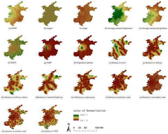
Figure 3. Driving factors affecting land use and land cover change in Beijing plain area.

3. Results

3.1. Spatiotemporal Changes in Carbon Sequestration

This study reported that the NPP in the central urban area had low values, but the surrounding areas had high values. In terms of temporal trend, the NPP initially showed decreasing trend followed by an increasing trend in the southern plain area. The central urban area showed a downward trend. Similarly, an overall decreasing trend in NPP was observed in the northern plain area, despite an upward trend since 2014. From 1999 to 2004, the NPP in the southeastern plain area showed a downward trend, followed by an upward trend. Generally speaking, with the development of the city, NPP in the Beijing plain area has changed (Figure 4).

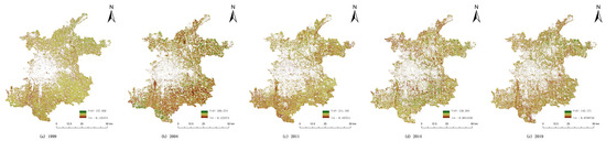
Figure 4. Monthly average NPP in plain areas of Beijing from 1999 to 2019.

3.2. Changes and Distribution Characteristics of Landscape Pattern Indices

This study analyzed land use changes in the Beijing plain areas from 1999 to 2019, focusing on five indicators (i.e., CONTAG, ED, SHEI, PRD, and LPI) that correlate well with NPP and reflect landscape fragmentation and diversity. Overall, the SHEI, ED, and PRD indices showed a decreasing trend, while the LPI and CONTAG showed an increasing trend. A decrease in the SHEI index in the suburban areas indicates that urbanization squeezed the advantage patches in the construction land, but the outer advantage patches became dominant. An increase in the CONTAG index indicates better connectivity between advantage patches. An increase in the PRD index was primarily reflected in the central urban area, where green space was decreased, but the richness and density of landscape patches increased. The growth of LPI indicates that the proportion of the largest patch in a certain patch type increased, reflecting the increase in advantage type and richness. The ED index showed a decreasing trend in the suburban areas but an increasing trend in the main urban areas, suggesting increased landscape fragmentation and complexity of the shapes. Overall, from 1999 to 2019, the landscape patterns within the urban construction land area showed a gradual trend toward fragmentation, dispersion, and homogenization, increasing the ecosystem vulnerability. However, the landscape patterns in suburban areas tended to be stable.

3.3. Correlation between Street Scale Carbon Sequestration and Landscape Pattern Indices

The relationships between landscape pattern indices and carbon sequestration at landscape and category levels were determined by creating scatter plots and calculating Pearson correlation coefficients (see Figure 5 and Figure 6, and Table 3). The significant relationships (p < 0.01) between landscape pattern indices and NPP (i.e., a surrogate for carbon sequestration) were observed; however, the relationships were complex, with some showing positive but others showing negative relationships. Results showed that the CA had a significant positive impact on NPP. We also studied the correlation between landscape pattern and NPP per unit area, compared it with spatial level, and subsequently built the multiple linear regression models.

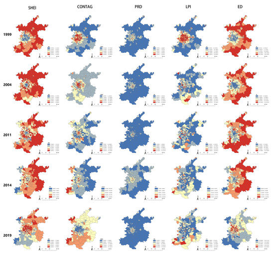
Figure 5. Changes in landscape pattern indices for the plain areas of Beijing from 1999 to 2019.

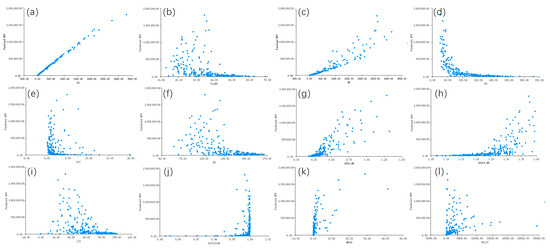
Figure 6. Scatter plots showing correlation between cultivated land landscape pattern indices and NPP. Note: (a) CA, (b) PLAND, (c) NP, (d) PD, (e) LPI, (f) ED, (g) AREA_MN, (h) SHAPE_MN, (i) IJI, (j) DIVISION, (k) MESH, (l) SPLIT.

Table 3. Correlation between landscape pattern and carbon sink.

Pearson Correlation	Landscape Indexes	CA	PLAND	NP	PD	LPI	ED	AREA_MN	SHAPE_MN	IJI	DIVISION	MESH	SPLIT
Category	NPP of grassland	0.942 **	0.534 **	0.859 **	−0.606 **	0.348 **	−0.224 **	0.808 **	0.699 **	0.203 *	−0.330 **	0.783 **	−0.352 **
	NPP of farmland	0.901 **	−0.437 **	0.935 **	−0.637 **	−0.079	−0.530 **	0.852 **	0.652 **	−0.483 **	0.194 *	0.633 **	0.244 **
	NPP of forestland	0.936 **	0.318 **	0.866 **	−0.458 **	−0.143 *	0.162 *	0.649 **	0.658 **	−0.621 **	0.076 *	0.435 **	0.001
	NPP per unit area of grassland		0.538 **	0.578 **	−0.690 **	0.439 **	−0.061	0.547 **	0.694 **	0.406 **	−0.386 **	0.367 **	−0.428 **
	NPP per unit area of farmland		−0.112	−0.357 **	0.170 **	−0.253 **	−0.222 **	−0.417 **	−0.132	−0.117	−0.248 **	0.102	−0.110
	NPP per unit area of forestland		0.373 **	0.535 **	−0.671 **	−0.014	0.189 **	0.642 **	0.739 **	−0.643 **	0.017	0.374 **	−0.112
Pearson correlation	landscape indexes	TA	LPI	ED	CONTAG	PRD	SHDI	SHEI
Landscape	NPP of landscape	0.923 **	0.176 *	−0.379 **	0.427 **	−0.281 **	−0.110 *	−0.110 *
	NPP per unit area of landscape		0.257 **	−0.108	0.150 *	−0.413 **	0.251 **	0.251 **

Note: ** indicates significant correlation at the 0.01 level (two-tailed), * indicates significant correlation at the 0.05 level (two-tailed).

At the category level, we found forests, croplands, and grasslands highly correlated with landscape pattern indices (p < 0.05) (Table 3, Figure 6, Figure 7 and Figure 8). Specifically, in terms of area and edge metrics, CA and AREA_MN showed significant correlations with NPP. PLAND had a significant negative correlation with croplands. In grasslands, LPI had a significant positive correlation with NPP, while in croplands, ED had a strong negative correlation with NPP. These results indicate that the larger the landscape area, the higher the NPP. For instance, grasslands with large patches and better connectivity can have higher NPP, and low fragmentation of boundaries can increase carbon sequestration in croplands.

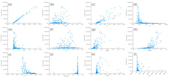
Figure 7. Scatter plots showing correlation between forest landscape pattern indices and NPP. Note: (a) CA, (b) PLAND, (c) NP, (d) PD, (e) LPI, (f) ED, (g) AREA_MN, (h) SHAPE_MN, (i) IJI, (j) DIVISION, (k) MESH, (l) SPLIT.

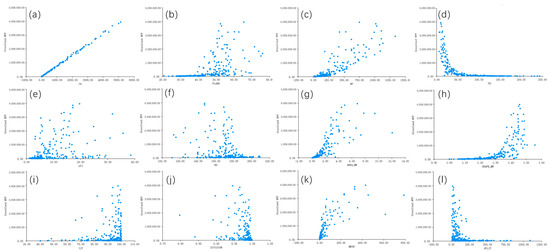
Figure 8. Scatter plots showing correlation between grassland landscape pattern indices and NPP. Note: (a) CA, (b) PLAND, (c) NP, (d) PD, (e) LPI, (f) ED, (g) AREA_MN, (h) SHAPE_MN, (i) IJI, (j) DIVISION, (k) MESH, (l) SPLIT.

Regarding density metrics, there was a strong positive correlation between NPP and NP and a negative correlation between NPP and PD, indicating that the higher number of green space patches with low fragmentation results in higher NPP. The shape metrics showed a strong positive correlation with NPP, suggesting that the complex patch shape may support higher NPP. For aggregation metrics, DIVISION and SPLIT showed a strong negative correlation with NPP in grassland. In contrast, the IJI showed a positive correlation with NPP. In forest and cropland, IJI showed a negative correlation with NPP. Finally, MESH showed a strong positive correlation with NPP in all categories. These results suggest that low fragmentation and aggregated large patches likely contribute to higher carbon sequestration. In croplands, high density and connectivity among cropland patches lead to higher NPP. Nevertheless, a higher proportion of green space in the landscape contributes to higher NPP. In grassland, after removing the effect of CA, the correlation between IJI and LPI with NPP increased, while the correlation between ED and NPP decreased.

In the cropland, after removing the effect of CA, the correlation between LPI and DIVISION strengthened, while the correlations of other indices were weakened. In the forest, the correlation between PD and SHAPE slightly increased after removing the effect of CA, while the other correlations did not change significantly. At landscape level, there was a significant correlation between landscape indices and NPP (Table 3, Figure 9). TA, LPI, and CONYAG were positively correlated with NPP. Landscape area was one of the main factors affecting NPP; landscapes with larger core patches and better connectivity had higher NPP. In contrast, the ED, PRD, SHDI, and SHEI were negatively correlated with NPP. These results suggest that landscape patches with low boundary density, more aggregation, and less fragmentation may have higher NPP. After excluding the influence of TA, the correlation between ED and CONYAG decreased, whereas the other correlations increased.

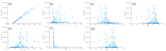
Figure 9. Scatter plots showing correlation between landscape pattern indices and NPP at landscape level. Note: (a) TA, (b) LPI, (c) ED, (d) SHEI, (e) CONTAG, (f) FRD, (g) SHDI.

3.4. Multiple Linear Regression Models

There was positive and negative correlation between the landscape pattern indices and NPP at street scale. Stepwise multiple linear regression models were developed, based on changes in correlation coefficients after removing CA, to determine the effects of landscape patterns on carbon sequestration efficiency at the category level. Across the green space categories (i.e., forest, grassland, and cropland), the regression models were developed using 11 landscape pattern indices as independent variables and street-scale NPP and unit area NPP as dependent variables. A total of 237 data sets were analyzed. When necessary, the data were log transformed to achieve homogeneity of variance before the analysis.

3.4.1. Linear Regression Model for Forestland

Stepwise multiple regression with an automatic selection process identified a final model with six variables (PLAND, NP, AREA_MN, ln(NP), ln(AREA_MN), and ln(DIVISION)) explaining 92.20% variation in street-scale NPP (adjusted R² = 0.922) (Table 4). The F-test results showed the overall significance of the regression model (F = 449.708, p = 0.000) (Table 4). The selected variables had significant positive impact on street-scale NPP. The regression model was built as follows:

NPP = −379,231.030 + 8577.350PLAND + 1246.084NP + 589,790.797AREA_MN − 69,921.814ln(NP) − 234,213.437ln(AREA_MN) + 8,165,904.152ln(DIVISION).

Table 4. Stepwise multiple linear regression showing model fit for street-scale NPP in forestland.

Stepwise Regression Analysis Results (n = 237)
	Nonstandardized coefficient		Standardization coefficient	t	p	VIF
	B	Standard error	Beta
constant	−379,231.030	86,544.267	-	−4.382	0.000 **	-
PLAND	8577.350	1511.447	0.178	5.675	0.000 **	2.896
NP	1246.084	50.846	0.828	24.507	0.000 **	3.342
AREA_MN	589,790.797	38,018.109	0.785	15.513	0.000 **	7.501
ln(NP)	−69,921.814	13,272.527	−0.212	−5.268	0.000 **	4.751
ln(AREA_MN)	−234,213.437	33,983.898	−0.368	−6.892	0.000 **	8.362
ln(DIVISION)	8,165,904.152	570,699.077	0.386	14.309	0.000 **	2.127
R2	0.922
Adjusted R2	0.920
F	F (6229) = 449.708, p = 0.000
Durbin–Watson	1.746

** p < 0.01.

With respect to unit area NPP, the final model identified four variables, LPI, PD, PLAND, and ln(pland), explaining 76.6% of the variance (adjusted R² = 0.766) in average NPP (Table 5). The F-test results showed that the overall regression model was statistically significant (F = 189.550, p = 0.000), and these variables had a negative impact on unit area NPP. The model was built as follows:

NPP per unit area = 801.811 − 4.265LPI − 3.973PD − 2.972PLAND + 160.754ln(pland).

Table 5. Stepwise multiple linear regression showing model fit for per unit area NPP in forestland.

Stepwise Regression Analysis Results (n = 237)
	Nonstandardized coefficient		Standardization coefficient	t	p	VIF
	B	Standard error	Beta
constant	801.811	32.264	-	21.969	0.000 **	-
LPI	−4.265	0.964	−0.216	−4.423	0.000 **	2.351
PD	−3.973	0.180	−0.768	−22.098	0.000 **	1.196
PLAND	−2.972	1.319	−0.279	−2.252	0.025 *	15.167
ln(pland)	160.754	19.561	0.892	8.218	0.000 **	11.655
R2	0.766
Adjusted R2	0.762
F	F (4232) = 189.550, p = 0.000
Durbin–Watson	2.230

* p < 0.05, ** p < 0.01.

3.4.2. Linear Regression Model for Farmland

Stepwise multiple linear regression models followed by automatic selection identified five variables (NP, SPLIT, LPI, SHAPE_MN, and PLAND), explaining 92.10% variance in NPP (R² = 0.921) at street-scale NPP (Table 6). The F-test showed that the overall regression was statistically significant (F = 535.964, p = 0.000 < 0.05) (Table 6), indicating that the selected variables significantly explained the variation in NPP. The regression model was constructed as follows: NPP = −684,006.439 + 472.015NP − 17.013SPLIT + 6745.262LPI + 429,015.388SHAPE_MN + 2486.141 × PLAND.

Table 6. Stepwise multiple linear regression showing model fit for street-scale NPP in farmland.

Stepwise Regression Analysis Results (n = 237)
	Nonstandardized coefficient		Standardization coefficient	t	p	VIF
	B	Standard error	Beta
constant	−684,006.439	157,573.327	-	−4.341	0.000 **	-
NP	472.015	12.764	1.008	36.980	0.000 **	2.165
SPLIT	−17.013	2.402	−0.167	−7.083	0.000 **	1.615
LPI	6745.262	2936.626	0.050	2.297	0.023 *	1.372
SHAPE_MN	429,015.388	119,347.657	0.094	3.595	0.000 **	1.992
PLAND	2486.141	829.146	0.088	2.998	0.003 **	2.504
R2	0.921
Adjusted R2	0.919
F	F (5231) = 535.964, p = 0.000
Durbin–Watson	1.692

* p < 0.05, ** p < 0.01.

Regarding the individual contribution, NP, LPI, SHAPE_MN, and PLAND showed a significant positive effect on NPP, while SPLIT had a significant negative effect.

Concerning per unit area NPP, the regression model identified seven variables, PD, PLAND, AREA_MN, IJI, ln(IJI), MESH, and ln(MESH), explaining 44.60% of the total variation in NPP per unit area (Table 7). The F-test showed that the overall regression was statistically significant (F = 26.189, p = 0.000) (Table 7), indicating that selected variables effectively explained the variation in NPP. The regression model was built as follows:

NPP per unit area = 519.558 − 0.461PD + 1.228PLAND − 105.531AREA_MN − 1.910IJI + 68.269ln(IJI) + 1.463MESH − 14.049 × ln(MESH).

Table 7. Multiple linear regression showing model fit with respect to per unit area NPP in farmland.

Stepwise Regression Analysis Results (n = 237)
	Nonstandardized coefficient		Standardization coefficient	t	p	VIF
	B	Standard error	Beta
constant	519.558	47.694	-	10.893	0.000 **	-
PD	−0.461	0.104	−0.929	−4.437	0.000 **	8.033
PLAND	1.228	0.450	0.439	2.729	0.007 **	5.626
AREA_MN	−105.531	21.804	−0.668	−4.840	0.000 **	7.846
IJI	−1.910	0.328	−1.281	−5.822	0.000 **	9.909
ln(IJI)	68.269	15.297	0.910	4.463	0.000 **	7.102
MESH	1.463	0.602	0.183	2.428	0.016 *	2.332
ln(MESH)	−14.049	3.619	−0.536	−3.882	0.000 **	7.847
R2	0.446
Adjusted R2	0.429
F	F (7228) = 26.189, p = 0.000
Durbin–Watson	2.085

* p < 0.05, ** p < 0.01.

Regression analyses also showed that PLAND and MESH had significant positive impacts on per unit area NPP. In contrast, PD, AREA_MN, and IJI had a significant negative impact.

3.4.3. Linear Regression Models for Grassland

For the grassland category, the regression model identified four variables, PLAND, NP, AREA_MN, and MESH, explaining 93.80% of the total variance in street-scale NPP (R² = 0.938) (Table 8). The F-test showed that the overall regression was statistically significant (F = 883.913, p = 0.000) (Table 8), indicating that the model effectively explained the NPP. The model was built as follows:

Table 8. Stepwise multiple linear regression showing model fit for street-scale NPP in grassland.

Stepwise Regression Analysis Results (n = 237)
	Nonstandardized coefficient		Standardization coefficient	t	p	VIF
	B	Standard error	Beta
constant	11,040.534	76,135.006	-	2.772	0.006 **	-
PLAND	−12,948.604	1981.646	−0.169	−6.534	0.000 **	2.511
NP	1821.443	60.967	0.589	29.876	0.000 **	1.466
AREA_MN	208,839.111	18,852.946	0.428	11.077	0.000 **	5.626
MESH	1999.723	263.014	0.225	7.603	0.000 **	3.304
R2	0.938
Adjusted R2	0.937
F	F (4232) = 883.913, p = 0.000
Durbin–Watson	1.427

** p < 0.01.

NPP = 11,040.534 − 12,948.604PLAND + 1821.443NP + 208,839.111AREA_MN + 1999.723MESH. Results also showed that NP, AREA_MN, and MESH had a significant positive impact on NPP, whereas PLAND had a significant negative impact.

Regarding per unit area NPP, six variables, NP, LPI, AREA_MN, SHAPE_MN, IJI, and MESH, explained 61.30% of the total variance in per unit area NPP (R² = 0.613) (Table 9). The F-test showed that the overall regression was statistically significant (F = 60.847, p = 0.000) (Table 9), indicating that the model effectively explained the variation in per unit area NPP. The model was built as follows:

NPP per unit area = 535.841 + 0.049NP + 2.082LPI + 5.502AREA_MN + 51.105SHAPE_MN + 1.133IJI − 0.126MESH.

Table 9. Stepwise multiple linear regression showing model fit for per unit area NPP in grassland.

Stepwise Regression Analysis Results (n = 237)
	Nonstandardized coefficient		Standardization coefficient	t	p	VIF
	B	Standard error	Beta
constant	535.841	32.047	-	16.72	0.000 **	-
NP	0.049	0.010	0.328	4.683	0.000 **	2.923
LPI	2.082	0.327	0.376	6.371	0.000 **	2.070
AREA_MN	5.502	2.395	0.236	2.297	0.023 *	6.260
SHAPE_MN	51.105	29.347	0.162	1.741	0.083	5.140
IJI	1.133	0.166	0.311	6.809	0.000 **	1.241
MESH	−0.126	0.036	−0.296	−3.470	0.001 **	4.343
R2	0.613
Adjusted R2	0.603
F	F (6230) = 60.847, p = 0.000
Durbin–Watson	1.859

* p < 0.05, ** p < 0.01.

Regression results showed significant positive effects of NP, LPI, AREA_MN, and IJI on per unit area NPP. In contrast, MESH showed a significant negative impact.

3.5. Accuracy Test of Linear Regression Models

The performance of the category-level models in explaining NPP was tested by performing a linear regression between the predicted and the actual NPP for 2014. Results showed a strong correlation between the predicted and actual NPP (e.g., Table 10, Figure 10). The adjusted R² values of the regression models for the predicted and actual values of the three predictive models were between 0.849 and 0.992, and the average RMSE values were between 0.016 and 0.028. These results indicated that the prediction accuracy of the category-level prediction models was high, and the linear relationship between the predicted and the actual values was distinct, with slopes close to 1.

Table 10. Accuracy test of multivariate linear regression model (t/C).

Model	R	R2	Adjusted R2	RMSE	Durbin–Watson
Model for forestland	0.849	0.848	0.028	1.556	y = −0.197 + 1.109x
Model for farmland	0.902	0.902	0.013	1.893	y = −0.0385 + 0.725x
Model for grassland	0.896	0.896	0.021	1.924	y = 0.0998 + 0.961x

Note: The accuracy test was conducted by comparing the predicted and actual values of 237 streets in 2014. R² is the coefficient of determination, and RMSE is the root mean square error.

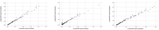
Figure 10. Scatter plot showing the predicted and actual NPP values for different categories.

3.6. Scenario Setting and Analysis of the FLUS Model

3.6.1. Land Use Analysis Based on Different Scenarios

Using 2014 land use data from the Beijing plain area, the FLUS model was developed to simulate the land use pattern in 2019. The simulation results were then verified with the actual land use data from 2019 using a kappa index. The kappa coefficient of the FLUS model was 0.86, which is greater than 0.75, indicating a high simulation accuracy for land use changes in the Beijing plain area.

This study set different conversion costs and domain coefficients using simulation results and four development scenarios. The BD scenario continued the current development trend, and its conversion costs and domain coefficients were determined based on existing research. Under the rapidly developing FD scenario, urbanization further accelerated. The study strengthened the expansion of construction land to other land use under this scenario and changed the conversion cost and domain coefficient accordingly. The LD scenario develops slowly. The study sets its GDP growth and urbanization development degree at 80.00% of the BD scenario to adjust the corresponding transformation cost and domain factors. For the SD scenario, the study restricted the transfer of forestland to other land use types. It promoted the transfer of unused land to forestland and grassland to adjust the conversion cost and domain coefficient. Using these scenarios for 2019 land use data, the FLUS model was used to simulate the spatiotemporal changes in land use distribution for 2034 (Figure 11).

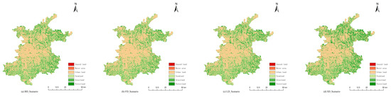
Figure 11. Simulated land use map of the Beijing plain area for 2034.

Simulation results showed decreasing trends in unused land, grassland, and water areas but an increasing trend in cultivated land under all four scenarios (Table 10). Under the SD scenario, unused land decreased the most, while grassland decreased the least. Under the FD scenario, the water area decreased the most. Under the BD, LD, and SD scenarios, the cultivated land area increased the most. However, under the FD scenario, construction land increased significantly. Under the BD and LD scenarios, construction land remained unchanged and slightly increased from 2019, respectively, for the BD and LD scenarios. Under the SD scenario, construction land was slightly reduced as the controlled measures were applied. Regarding forestland, a decreasing trend was observed under the BD, FD, and LD scenarios. The most dramatic changes were observed under the FD scenario as construction land expanded rapidly. In contrast, under the SD scenario, forestland, grassland, and water areas were well protected and showed increasing trends. For example, in the northern and southern parts of the study area, the forestland cover increased under the SD scenario compared to other scenarios (Table 11, Table 12, Table 13 and Table 14).

Table 11. Conversion of land use types in the Beijing plain area from 2019 to 2034 under the BD scenario (km²).

2019–2034 BD	Unused Land	Water Area	Urban Land	Farmland	Grassland	Forestland	Total
Unused land	1.7433	0.8361	0.1845	3.1959	0.0045	0	5.9643
Water area	0	52.3413	0	12.7575	0.0504	0	65.1492
Urban land	0	0	2474.7435	0	0	0	2474.7440
Farmland	0	0	0.0009	968.3910	0.0072	0	968.3991
Grassland	0	0	4.8177	252.2511	1885.9230	15.2595	2158.2510
Forestland	0	0	0.4041	245.1402	26.8236	458.4330	730.8009
Total	1.7433	53.1774	2480.1507	1481.7360	1912.8090	473.6925	6403.3080

Table 12. Conversion of land use types in the Beijing plain area from 2019 to 2034 under the FD scenario (km²).

2019–2034 FD	Unused Land	Water Area	Urban Land	Farmland	Grassland	Forestland	Total
Unused land	1.6371	0.1575	1.4265	2.7288	0.0135	0.0009	5.9643
Water area	0	50.9931	11.5236	2.6325	0	0	65.1492
Urban land	0	0	2474.7435	0	0	0	2474.744
Farmland	0	0	70.3503	889.8570	8.1477	0.0441	968.3991
Grassland	0	0.0576	63.3420	333.8343	1708.4710	52.5465	2158.2510
Forestland	0	0	7.2639	230.4126	172.6542	320.4702	730.8009
Total	1.6371	51.2082	2628.6498	1459.4650	1889.2860	373.0617	6403.3080

Table 13. Conversion of land use types in the Beijing plain area from 2019 to 2034 under the LD scenario (km²).

2019–2034 LD	Unused Land	Water Area	Urban Land	Farmland	Grassland	Forestland	Total
Unused land	1.6542	1.1295	0.0405	3.1383	0.0018	0	5.9643
Water area	0	51.363	0	13.7268	0.0504	0.0090	65.1492
Urban land	0	0	2474.7435	0	0	0	2474.7440
Farmland	0	0.4959	4.3119	945.4329	18.1440	0.0144	968.3991
Grassland	0	0.0756	0.9720	268.9110	1868.0660	20.2266	2158.2510
Forestland	0	0.1134	0.0837	250.5735	26.5851	453.4452	730.8009
Total	1.6542	53.1774	2480.1516	1481.7830	1912.8470	473.6952	6403.3080

Table 14. Conversion of land use types in the Beijing plain area from 2019 to 2034 under the SD scenario (km²).

2019–2034 SD	Unused Land	Water Area	Urban Land	Farmland	Grassland	Forestland	Total
Unused land	1.3374	0.2313	4.2921	0.1008	0.0027	0	5.9643
Water area	0	51.921	0	13.1562	0.0657	0.0063	65.1492
Urban land	0	0.1656	2460.4893	5.9184	7.9074	0.2628	2474.7440
Farmland	0	0.7596	0	944.8389	22.8006	0	968.3991
Grassland	0	0.0999	0	258.7941	1882.0640	17.2935	2158.2510
Forestland	0	0	0	0	0	730.8009	730.8009
Total	1.3374	53.1774	2464.7814	1222.8080	1912.8404	748.3635	6403.3080

3.6.2. Landscape Pattern Index Analysis

Applying the four development scenarios, this study simulated the land use change and spatial distribution patterns in the Beijing plain area for 2034. However, some landscape indices showed regional differences due to the complex topographical structure and climatic conditions. The SHEI index showed that the difference between the BD and SD scenarios was greater than between the FD and LD scenarios, indicating that the SD and BD scenarios could generate more dominant landscape patches. The CONTAG index showed that the difference in the FD scenario was greater than in the BD, SD, and LD scenarios in 2034, suggesting that rapid development may reduce the connectivity of advantageous patches, leading to aggregation patterns of multiple land types. The PRD index highlighted the differences in the main urban area under different development scenarios, with a higher landscape density under the BD and SD scenarios. The LPI index showed no significant differences across the BD, SD, and FD scenarios. However, it was relatively lower in the FD scenario, indicating a decrease in the proportion of the largest patches in the landscape. The ED index showed significant differences in the FD scenario, indicating that patches were fragmented, boundaries were disrupted, and the landscape became fragmented. Across the four scenarios, the landscape fragmentation in the BD and SD scenarios was lower than that in the FD and LD scenarios, and the fragmentation in the central urban area was higher than that in the suburbs (Figure 12).

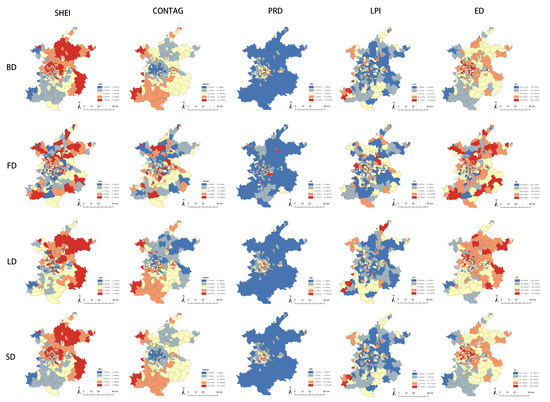
Figure 12. Changes in landscape pattern in the Beijing plain area under four development scenarios (BD, FD, SD, and LD).

3.7. Carbon Sink Simulation Prediction

Multiple linear regression models were developed to predict the carbon sink capacity of green spaces (i.e., land use types) under each development scenario (e.g., Table 15, Figure 13a). Additionally, the per unit area NPP prediction model was used to make predictions (e.g., Table 16, Figure 13b). Results showed that the carbon sink prediction trends for both models were consistent (e.g., Table 15 and Table 16).

Table 15. Monthly NPP prediction for the Beijing plain area from 2014 to 2034 based on the category-level NPP regression model (g/C).

Year	Scenario	Forestland	Farmland	Grassland
2014		54,250,654.55	34,040,262.67	107,358,964.70
2019		58,163,638.07	47,998,134.52	119,078,547.80
2034	BD	39,841,449.45	59,542,375.34	108,855,603.40
	FD	33,587,139.56	56,469,129.76	97,947,988.55
	LD	38,126,008.13	60,138,195.03	109,207,321.10
	SD	62,982,188.67	50,657,066.10	110,479,376.70

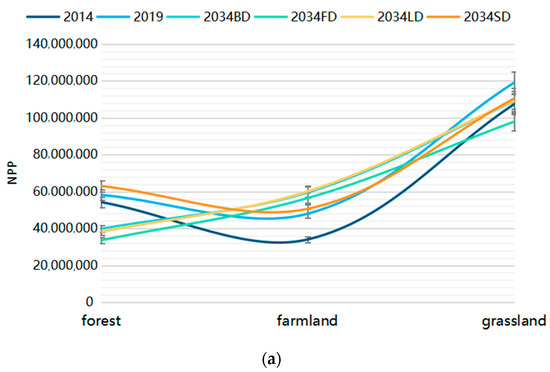
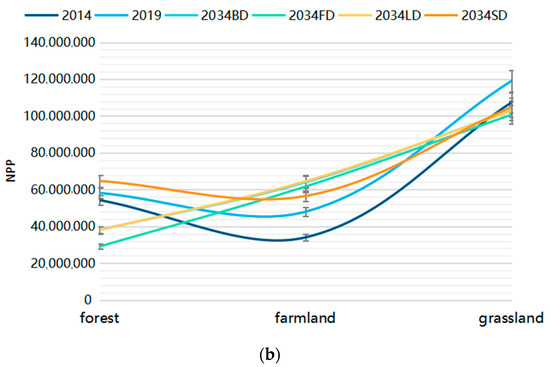
Figure 13. (a) Monthly NPP prediction for the Beijing plain area from 2014 to 2034 based on the category-level NPP regression model. (b) Monthly NPP prediction for the Beijing plain area from 2014 to 2034 based on the unit area-level NPP regression model.

Table 16. Monthly NPP prediction for the Beijing plain area from 2014 to 2034 based on the unit area-level NPP regression model (g/C).

Year	Scenario	Forestland	Farmland	Grassland
2014		54,250,654.55	34,040,262.67	107,358,964.70
2019		58,163,638.07	47,998,134.52	119,078,547.80
2034	BD	38,075,182.27	64,051,665.18	103,062,021.40
	FD	29,073,077.89	61,673,465.98	100,692,794.50
	LD	37,957,412.14	64,534,348.02	102,734,456.10
	SD	64,692,688.54	56,529,609.02	104,809,356.50

Considering the four development scenarios, the NPP was the highest under SD, followed by BD, LD, and FD. Regarding land use types, grassland had the highest NPP, followed by farmland and forestland. Overall, in the forestland, NPP showed an increasing trend from 2014 to 2019, but under the BD, LD, and FD scenarios, NPP showed a decreasing trend for 2034. The decrease was most pronounced under the FD scenario, with a decline of more than 40.00%. However, under the SD scenario, NPP showed an increasing trend. A comparative analysis showed that the NPP values under the BD, FD, and LD scenarios exceeded the NPP per unit area. The NPP prediction under the BD, FD, and LD scenarios was greatly affected by NP, AREA_MN, and DIVISION, while LPI and PD influenced the per unit area NPP prediction.

Farmland showed a sustained upward trend under all four scenarios, with the largest increase observed under the LD scenario. The model comparison showed that the NPP model predictions under all four scenarios were less than the NPP model per unit area. The former was primarily influenced by NP, SPLIT, LPI, and SHAPE_MN, while PD, AREA_MN, IJI, and MESH influenced the latter.

For the grassland, NPP showed an upward trend from 2014 to 2019. However, under the FD scenario and for 2034, NPP suffered the greatest decline. In contrast, under the SD scenario, NPP had the greatest increase. Under the BD, SD, and LD scenarios, the NPP model predictions were higher than the NPP model per unit area. A comparative analysis showed that PLAND influenced the NPP model prediction under the BD, SD, and LD scenarios, while the LPI, SHAPE_MN, and IJI influenced the outcome of the NPP model per unit area. Results from both models implied that carbon sequestration efficiency was optimal under the SD scenario.

4. Discussion

Under different development scenarios, this study compared NPP at street scale within the plain areas of Beijing in 2019 (Figure 14 and Figure 15). Results showed a significant difference in NPP between the FD and the SD scenarios. Future NPP under the FD scenario across most streets showed a downward trend, while the opposite results were observed under the SD scenario. Compared with 2019, in 2034, the differences in NPP between the BD and LD scenarios were insignificant. Their NPP values were intermediate between the FD and SD scenarios. These results suggest that the SD scenario may increase carbon sequestration and help toward achieving carbon neutrality goals. However, under the SD scenario, the NPP in the new urban land developments showed a downward trend [5]. The new urban land developments are important for manufacturing and agriculture. The assessment of green space patterns and NPP in Beiqijia, Baishan, and Xiaotangshan towns suggests that high landscape diversity, connectivity, number of dominant patches, and low landscape fragmentation likely explain the relatively high NPP in these towns. Therefore, new urban land developments should promote the layout and development of modern agriculture and strengthen the patch density by connecting cultivated land. In addition, attention should be given to protect forest and grassland, regulate construction land, and build a mosaic of landscape patches that reduces the degree of green space fragmentation.

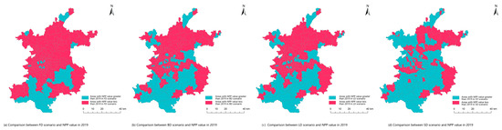
Figure 14. NPP increase and decrease in the Beijing plain area under four development scenarios (BD, FD, SD, and LD).

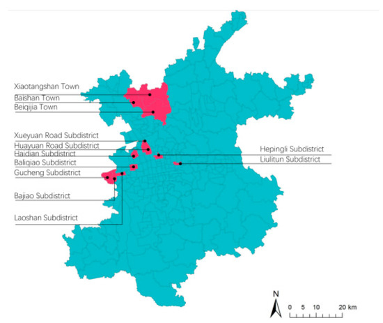
Figure 15. Typical street index map of the Beijing plain area.

The main urban area [5], with construction land as a primary land use type, had higher NPP under the SD scenario. Indeed, some of the streets, Haidian, Xuexue, and Huayuan roads, support more pointlike and striplike rich forest and grassland with higher landscape diversity, connectivity, and less fragmentation under the SD scenario, providing a conducive environment for higher NPP. Therefore, streets within the main urban area should be prioritized to increase green spaces, strengthen forest and grassland protection, and control construction land expansion. Additionally, it is possible to further integrate urban green spaces, such as the Olympic Forest Park, to create ecofriendly green spaces, enhance connectivity to the urban green network, and increase green space area.

However, the NPP of some neighborhoods showed declining trends under all four scenarios. Slowing the trend when the decline is seen under all four scenarios is particularly important. For example, an internal development imbalance has been observed in the urban functional expansion area [36]. In addition, streets in the northeast part of the city (e.g., Hepingli, Liulitun, and Balizhuang) experienced rapid urbanization, including a continuous reduction in advantageous landscape patches and increased fragmentation, resulting in NPP loss. However, slowing construction intensity and further integration of green core areas to build advantageous landscapes, create friendly green spaces, and enhance connectivity is necessary to reduce NPP loss. Similarly, the streets on the southwest side of the city (Rugucheng, Bajiao, and Laoshan) are also experiencing NPP loss due to increasing fragmentation despite better landscape connectivity. Particularly for the southwest side, implementing sustainable development practices, such as strengthening the construction of large central green spaces, protecting forests, maintaining the sustainable expansion of cultivated land, and reducing unused land, may reduce the intensity of NPP loss.

In contrast to previous research, this study investigated the impact of future land use changes and landscape patterns under different development scenarios on NPP. Different from previous studies that used NPP per unit area of different land use types in historical years as the reference value [24] to predict the spatiotemporal changes in NPP under multiple scenarios, this study is based on the correlation between landscape pattern indices at street scale and NPP. Multiple linear regression equations of total NPP and landscape pattern indices and per unit area NPP and landscape pattern indices were established. The regression models were then used to predict future changes in NPP under future landscape patterns and different development scenarios. The study also compared the effects of street-scale landscape patterns on overall NPP and per unit area NPP. The methodological approaches utilized in this study improved the accuracy and effectiveness of NPP prediction. These approaches also helped better explain the response of NPP to landscape patterns. Additionally, it will help policymakers formulate more targeted strategies for landscape pattern optimization, which have the potential to significantly enhance the carbon sequestration effectiveness of green spaces in the plain areas of Beijing and make a significant contribution to achieving carbon neutrality.

5. Conclusions

This paper uses a multimodel fusion research framework to explore the mechanism driving the landscape pattern of carbon sink at street level in the Beijing plain area from 1999 to 2019. The study further analyzed the response of carbon sequestration to landscape pattern changes and established a predictive model. Overall, the NPP of the region showed a downward trend. The landscape patterns in the Beijing plain area trended toward fragmentation, dispersion, and less diversity, increasing the ecosystem fragility. The predicted NPP under different development scenarios in 2034 showed that the NPP increased only in the forest category under the SD scenario. However, cultivated land increased under all four development scenarios. Interestingly, the NPP decreased in grassland under the SD scenario. Overall, improved carbon sink performance was reported across all categories under the SD scenario, suggesting that optimizing the street-level green space pattern in the Beijing plain area can drive NPP and carbon sequestration. Although evaluating the carbon sink performance of various land use types based solely on landscape patterns has limitations, the findings of this research still have important implications for optimizing the green space patterns in megacities to increase carbon sinks. Moreover, future research efforts should focus on studying the synergistic effects of combining landscape pattern optimization with other ecological restoration measures to maximize the carbon sink performance and overall sustainability of megacity urban green spaces.

References

- Mao, D.H.; Luo, L.; Wang, Z.M.; Zhang, C.H.; Ren, C.Y. Variations in net primary productivity and its relationships with warming climate in the permafrost zone of the Tibetan Plateau. J. Geogr. Sci. 2015, 25, 967–977. [Google Scholar] [CrossRef]
- Wei, W.D.; Hao, S.J.; Yao, M.T.; Chen, W.; Wang, S.S.; Wang, Z.Y.; Wang, Y.; Zhang, P.F. Unbalanced economic benefits and the electricity-related carbon emissions embodied in China’s interprovincial trade. J. Environ. Manag. 2020, 263, 110390. [Google Scholar] [CrossRef] [PubMed]
- Cramer, W.; Guiot, J.; Fader, M.; Garrabou, J.; Gattuso, J.P.; Iglesias, A.; Lange, M.A.; Lionello, P.; Llasat, M.C.; Paz, S.; et al. Climate change and interconnected risks to sustainable development in the Mediterranean. Nat. Clim. Chang. 2018, 8, 972–980. [Google Scholar] [CrossRef]
- Song, W.; Deng, X. Effects of Urbanization-Induced Cultivated Land Loss on Ecosystem Services in the North China Plain. Energies 2015, 8, 5678–5693. [Google Scholar] [CrossRef]
- Guo, L.; Liu, R.; Shoaib, M.; Men, C.; Wang, Q.; Miao, Y.; Jiao, L.; Wang, Y.; Zhang, Y. Impacts of landscape change on net primary productivity by integrating remote sensing data and ecosystem model in a rapidly urbanizing region in China. J. Clean. Prod. 2021, 325, 129314. [Google Scholar] [CrossRef]
- Yue, C.; Ciais, P.; Houghton, R.A.; Nassikas, A.A. Contribution of land use to the interannual variability of the land carbon cycle. Nat. Commun. 2020, 11, 3170. [Google Scholar] [CrossRef]
- Cao, M.K.; Prince, S.D.; Small, J.; Goetz, S.J. Remotely sensed interannual variations and trends in terestrial net primary productivity 1981–2000. Ecosystems 2004, 7, 233–242. [Google Scholar] [CrossRef]
- Wei, X.; Yang, J.; Luo, P.; Lin, L.; Lin, K.; Guan, J. Assessment of the variation and influencing factors of vegetation NPP and carbon sink capacity under different natural conditions. Ecol. Indic. 2022, 138, 108834. [Google Scholar] [CrossRef]
- Wang, Z.; Xu, L.H.; Shi, Y.J.; Ma, Q.W.; Wu, Y.Q.; Lu, Z.W.; Mao, L.W.; Pang, E.Q.; Zhang, Q. Impact of Land Use Change on Vegetation Carbon Storage during Rapid Urbanization: A Case Study of Hangzhou, China. Chin. Geogr. Sci. 2021, 31, 209–222. [Google Scholar] [CrossRef]
- Gao, Q.; Guo, Y.; Xu, H.; Ganjurjav, H.; Li, Y.; Wan, Y.; Qin, X.; Ma, X.; Liu, S. Climate change and its impacts on vegetation distribution and net primary productivity of the alpine ecosystem in the Qinghai-Tibetan Plateau. Sci. Total Environ. 2016, 554, 34–41. [Google Scholar] [CrossRef]
- Yang, H.F.; Zhong, X.N.; Deng, S.Q.; Xu, H. Assessment of the impact of LUCC on NPP and its influencing factors in the Yangtze River basin, China. Catena 2021, 206, 105542. [Google Scholar] [CrossRef]
- Wang, H.; Li, X.B.; Long, H.L.; Gai, Y.Q.; Wei, D.D. Monitoring the effects of land use and cover changes on net primary production: A case study in China’s Yongding River basin. For. Ecol. Manag. 2009, 258, 2654–2665. [Google Scholar] [CrossRef]
- Dong, G.T.; Bai, J.; Yang, S.T.; Wu, L.N.; Cai, M.Y.; Zhang, Y.C.; Luo, Y.; Wang, Z.W. The impact of land use and land cover change on net primary productivity on China’s Sanjiang Plain. Environ. Earth Sci. 2015, 74, 2907–2917. [Google Scholar] [CrossRef]
- Pei, F.S.; Li, X.; Liu, X.P.; Lao, C.H.; Xia, G.R. Exploring the response of net primary productivity variations to urban expansion and climate change: A scenario analysis for Guangdong Province in China. J. Environ. Manag. 2015, 150, 92–102. [Google Scholar] [CrossRef]
- Fu, Y.C.; Lu, X.Y.; Zhao, Y.L.; Zeng, X.T.; Xia, L.L. Assessment Impacts of Weather and Land Use/Land Cover (LULC) Change on Urban Vegetation Net Primary Productivity (NPP): A Case Study in Guangzhou, China. Remote Sens. 2013, 5, 4125–4144. [Google Scholar] [CrossRef]
- D’Eon, R.G.; Glenn, S.M. The influence of forest harvesting on landscape spatial patterns and old-growth-forest fragmentation in southeast British Columbia. Landsc. Ecol. 2005, 20, 19–33. [Google Scholar] [CrossRef]
- Asplund, M.E.; Dahl, M.; Ismail, R.O.; Arias-Ortiz, A.; Deyanova, D.; Franco, J.N.; Hammar, L.; Hoamby, A.I.; Linderholm, H.W.; Lyimo, L.D.; et al. Dynamics and fate of blue carbon in a mangrove-seagrass seascape: Influence of landscape configuration and land-use change. Landsc. Ecol. 2021, 36, 1489–1509. [Google Scholar] [CrossRef]
- Zhou, Y.Y.; Yue, D.X.; Guo, J.J.; Chen, G.G.; Wang, D. Spatial correlations between landscape patterns and net primary productivity: A case study of the Shule River Basin, China. Ecol. Indic. 2021, 130, 108067. [Google Scholar] [CrossRef]
- Gimeno, T.E.; Escudero, A.; Delgado, A.; Valladares, F. Previous Land Use Alters the Effect of Climate Change and Facilitation on Expanding Woodlands of Spanish Juniper. Ecosystems 2012, 15, 564–579. [Google Scholar] [CrossRef]
- Zhang, Y.L.; Qi, W.; Zhou, C.P.; Ding, M.J.; Liu, L.S.; Gao, J.G.; Bai, W.Q.; Wang, Z.F.; Zheng, D. Spatial and temporal variability in the net primary production of alpine grassland on the Tibetan Plateau since 1982. J. Geogr. Sci. 2014, 24, 269–287. [Google Scholar] [CrossRef]
- Yan, Y.C.; Liu, X.P.; Wang, F.Y.; Li, X.; Ou, J.P.; Wen, Y.Y.; Liang, X. Assessing the impacts of urban sprawl on net primary productivity using fusion of Landsat and MODIS data. Sci. Total Environ. 2018, 613, 1417–1429. [Google Scholar] [CrossRef] [PubMed]
- Liu, X.P.; Liang, X.; Li, X.; Xu, X.C.; Ou, J.P.; Chen, Y.M.; Li, S.Y.; Wang, S.J.; Pei, F.S. A future land use simulation model (FLUS) for simulating multiple land use scenarios by coupling human and natural effects. Landsc. Urban Plann. 2017, 168, 94–116. [Google Scholar] [CrossRef]
- Xiang, S.J.; Wang, Y.; Deng, H.; Yang, C.M.; Wang, Z.F.; Gao, M. Response and multi-scenario prediction of carbon storage to land use/cover change in the main urban area of Chongqing, China. Ecol. Indic. 2022, 142, 109205. [Google Scholar] [CrossRef]
- Jiang, X.W.; Bai, J.J. Predicting and assessing changes in NPP based on multi-scenario land use and cover simulations on the Loess Plateau. J. Geogr. Sci. 2021, 31, 977–996. [Google Scholar] [CrossRef]
- Zhu, W.; Pan, Y.; Yang, X.; Song, G. Comprehensive analysis of the impact of climatic changes on Chinese terrestrial net primary productivity. Chin. Sci. Bull. 2007, 52, 3253–3260. [Google Scholar] [CrossRef]
- Peng, J.; Shen, H.; Wu, W.; Liu, Y.; Wang, Y. Net primary productivity (NPP) dynamics and associated urbanization driving forces in metropolitan areas: A case study in Beijing City, China. Landsc. Ecol. 2016, 31, 1077–1092. [Google Scholar] [CrossRef]
- Uuemaa, E.; Mander, U.; Marja, R. Trends in the use of landscape spatial metrics as landscape indicators: A review. Ecol. Indic. 2013, 28, 100–106. [Google Scholar] [CrossRef]
- Ma, G.; Li, Q.; Yang, S.; Zhang, R.; Zhang, L.; Xiao, J.; Sun, G. Analysis of Landscape Pattern Evolution and Driving Forces Based on Land-Use Changes: A Case Study of Yilong Lake Watershed on Yunnan-Guizhou Plateau. Land 2022, 11, 1276. [Google Scholar] [CrossRef]
- Wang, H.R.; Zhang, M.D.; Wang, C.Y.; Wang, K.Y.; Wang, C.; Li, Y.; Bai, X.L.; Zhou, Y.K. Spatial and Temporal Changes of Landscape Patterns and Their Effects on Ecosystem Services in the Huaihe River Basin, China. Land 2022, 11, 513. [Google Scholar] [CrossRef]
- de Mello, K.; Taniwaki, R.H.; de Paula, F.R.; Valente, R.A.; Randhir, T.O.; Macedo, D.R.; Leal, C.G.; Rodrigues, C.B.; Hughes, R.M. Multiscale land use impacts on water quality: Assessment, planning, and future perspectives in Brazil. J. Environ. Manag. 2020, 270, 110879. [Google Scholar] [CrossRef]
- Khodakhah, H.; Aghelpour, P.; Hamedi, Z. Comparing linear and non-linear data-driven approaches in monthly river flow prediction, based on the models SARIMA, LSSVM, ANFIS, and GMDH. Environ. Sci. Pollut. Res. 2022, 29, 21935–21954. [Google Scholar] [CrossRef]
- Hamada, Y.; Zumpf, C.R.; Cacho, J.F.; Lee, D.; Lin, C.-H.; Boe, A.; Heaton, E.; Mitchell, R.; Negri, M.C. Remote Sensing-Based Estimation of Advanced Perennial Grass Biomass Yields for Bioenergy. Land 2021, 10, 1221. [Google Scholar] [CrossRef]
- O’Neill, B.C.; Kriegler, E.; Ebi, K.L.; Kemp-Benedict, E.; Riahi, K.; Rothman, D.S.; van Ruijven, B.J.; van Vuuren, D.P.; Birkmann, J.; Kok, K.; et al. The roads ahead: Narratives for shared socioeconomic pathways describing world futures in the 21st century. Glob. Environ. Chang.-Hum. Policy Dimens. 2017, 42, 169–180. [Google Scholar] [CrossRef]
- Wang, Z.Y.; Li, X.; Mao, Y.T.; Li, L.; Wang, X.R.; Lin, Q. Dynamic simulation of land use change and assessment of carbon storage based on climate change scenarios at the city level: A case study of Bortala, China. Ecol. Indic. 2022, 134, 108499. [Google Scholar] [CrossRef]
- Hishe, S.; Bewket, W.; Nyssen, J.; Lyimo, J. Analysing past land use land cover change and CA-Markov-based future modelling in the Middle Suluh Valley, Northern Ethiopia. Geocarto Int. 2020, 35, 225–255. [Google Scholar] [CrossRef]
- Wu, Q.; Tan, J.; Guo, F.; Li, H.; Chen, S. Multi-Scale Relationship between Land Surface Temperature and Landscape Pattern Based on Wavelet Coherence: The Case of Metropolitan Beijing, China. Remote Sens. 2019, 11, 3021. [Google Scholar] [CrossRef]
Disclaimer/Publisher’s Note: The statements, opinions and data contained in all publications are solely those of the individual author(s) and contributor(s) and not of MDPI and/or the editor(s). MDPI and/or the editor(s) disclaim responsibility for any injury to people or property resulting from any ideas, methods, instructions or products referred to in the content. |
© 2023 by the authors. Licensee MDPI, Basel, Switzerland. This article is an open access article distributed under the terms and conditions of the Creative Commons Attribution (CC BY) license (https://creativecommons.org/licenses/by/4.0/).