Comprehensive Evaluation of Land Use Planning Alternatives Based on GIS-ANP

Abstract

Planning alternatives evaluation is often influenced by the evaluator’s background knowledge and preferences, and its objectivity is hard to guarantee. A comprehensive evaluation method combining Geographic Information System (GIS) with system analysis technology is proposed in this paper. Using a land use issue in America as an example, GIS was combined with Fuzzy Logic, and the Analytic Network Process (ANP) method was used to evaluate three planning alternatives. The evaluation value of each qualitative index was obtained by Fuzzy Comprehensive Evaluation, and the quantitative index value was calculated by GIS algorithms. A weighted hypermatrix of ANP network was constructed to reveal the overall relative importance weight of alternatives. The results indicate that, in this case study, the factor weight rankings that influenced the selection of the land use alternative are Ecological factors (above 40%), socioeconomic factors (30%), Physical and Chemical factors (10–17%), and cumulative related factors (10%). In the long run, choices of planning alternatives will greatly affect the natural environment, the physical and chemical environment, and the social economy. The results indicate planners have to pay attention to a wide range of both qualitative and quantitative factors as much as possible in land use decisions. This study illustrates how the GIS-ANP method combine qualitative and quantitative factors in planning for a comprehensive analysis, thus improving the objectivity of evaluating land use planning alternatives and determining the importance of influencing factors. Future work aims to optimize the evaluation index system of planning, and measure index values in a more precise way.

1. Introduction

Land use planning is the inevitable requirement of urban development, and the comprehensive evaluation of planning alternatives plays a decisive role in determining the final urban layout.

The theoretical framework of planning evaluation proposed by the academic community has gradually become integrated and systematic, from initial analysis and evaluation only for planning alternatives [1] to the inclusion of citizen input into the planning process (directly or through representatives who participate in decisions that affect their lives, determining whether if and how plan will be applied) [2], and gradually developing a unified planning alternative evaluation and its standard (six principles used to evaluate comprehensive plans, including harmony with nature, equity, liveable built environments, etc.) [3]. The indicator system used in the evaluation of planning alternatives has also changed from a single measurement system, such as the Human Development Index (HDI) [4], the Physical Quality of Life Index (PQLI) [5], the Ecological Footprint (EF) [6], and the Barometer of Sustainability (BS) [7], to a greater focus on the common development of environmental systems and societal capacity, such as the Environmental Sustainability Index (ESI) [8], and the Sustainable Society Index (SSI) [9]. Environmental systems indicators are related to natural resources, such as the capacity of natural capital to sustain the supply of biotic and abiotic natural resources or to maintain ecosystem health and function as well as environmental sustainability that requires maintaining environmental functions [10]. Societal indicators, on the other hand, focus more on human and social aspects like human health and welfare, personal development and health including Education and Gender Equality; they also relate to economy like Gross Domestic Product (GDP), employment, and livelihoods.

Land use planning is a complex system, considering the complexity and diversity of indicator systems used in the alternatives evaluation mentioned above, let alone incorporating influencing factors that are composed of multiple elements and element groups with cross relationships, such as traffic, water systems, and ecology. In addition, economic and social indicators such as income, employment rate, and sustainable development are also critical factors in evaluating planning alternatives.

There are three common comprehensive evaluation modes of urban planning: the Parallel mode based on subsystem decomposition [11,12], the Vertical mode based on sustainable development as well as development and coordination ability [13,14], and the Pressure-State-Response (P-S-R) mode based on system dynamics [15]. The division of parallel and vertical evaluation systems is relatively simple, but it is difficult to determine the cross relationships among influencing factors and factor groups in planning; the P-S-R model can analyze the causal relationship between system factors, but it fails to classify indicators. Meanwhile, in the process of application, most of the index weighting methods are not sufficiently objective or not geographically related. For example, index weighting methods like Delphi, Fuzzy Comprehensive Evaluation, and Analytic Hierarchy Process (AHP) can be highly subjective [16], while objective index weighting methods such as the Entropy Method, Principal Component Analysis (PCA), Cluster Analysis, and Artificial Neural Network have little geographical relevance. It can be seen that common comprehensive evaluation modes have trouble determining the cross relationships among influencing factors while ensuring objectivity and geographical relevance at the same time.

Given the above, this study applies a comprehensive method for evaluating planning alternatives to the joint weighting of ANP and GIS spatial computing. Thus, the overall goal is to ensure the objectivity of the selected evaluation indicators incorporating a high degree of geographical relevance, to improve the credibility of the evaluation results. Through combination of a subjective evaluation index and an objective one, as well as a comprehensive analysis carried out by the system analysis method supported by computer technology, the proposed method is expected to increase the objectivity of land use planning alternative evaluation and, moreover, achieve the unity of subjectivity and objectivity of planning alternatives.

There are five parts to the paper: the first part, just presented, gives a brief introduction to the background of the problem; the second addresses the description of the research area and the evaluation index system method; then, the comprehensive evaluation method of GIS-ANP is presented, followed by the evaluation results. The last section includes the discussion and conclusions of the research.

2. Geographical Conditions of the Study Area

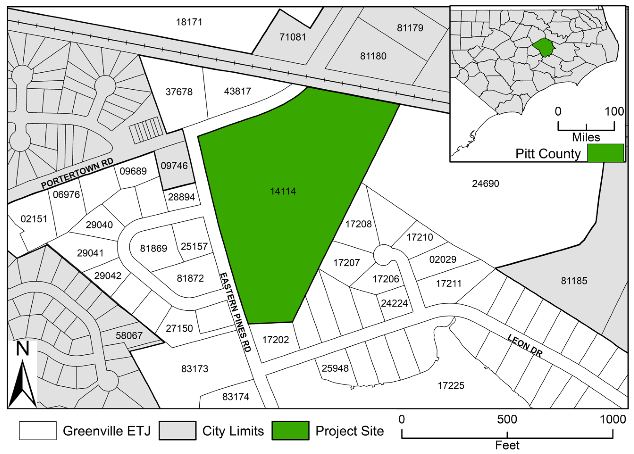
2.1. Location and Planning Alternatives

The study area is located in the urban fringe of Greenville in Pitt County, North Carolina. It is within the extra-territorial jurisdiction (ETJ) of Greenville and does not fall within the official city limits (Figure 1). Greenville represents a growing urban centre in eastern North Carolina with approximately 93,400 residents. The City of Greenville experiences a poverty rate of 31.4%, 8.2 percentage points greater than Pitt County as a whole, and the majority of residents rent their homes indicating that access to affordable housing should be considered in the evaluation process [17,18]. The surrounding area is serviced by municipal water and is located to the south of a large commercial development as well as several smaller retail and restaurant properties. Retail spending in Greenville was approximately USD 18,215 per capita in 2019, USD 4500 greater than the Pitt County average, indicating that commercial and retail development would likely be beneficial [17,18]. The surrounding residential properties are predominantly single-family residential and residential-agricultural zoning. The primary school that serves the study site is currently overcrowded, and additional enrolment would further strain the school resources [19].

The study plot is a 14.221 acre cleared vacant lot zoned as RA20 (Residential-Agricultural). The plot is bordered by a freight railway to the north and two major roadways to the west. The parcels north of the railway are commercial properties including retail and restaurant properties. South of the railway the area is predominantly single-family residential properties with a small number of multi-family units. The proposed development will subdivide the plot into 9.183 acres of R6 (High Density Residential) housing with the remaining 5.038 acres being converted to GC (General Commercial) zoning. The commercial portion is anticipated to include retail and restaurant businesses as well as human services, such as medical and legal offices, to provide additional service to the growing population in this area. The proposed rezoning is similar to land uses (mainly residential and supplemented by agricultural, without commercial use) surrounding the site, but questions remain about the impacts of further development in this area. The specific location (No. 14114) is shown in the green shaded area of Figure 1.

Three initial planning alternatives were proposed as described below, the first being the proposed action aimed to improve the local economy, the second an alternative aimed at reducing density and thus impacts, and the third to consider impacts of no change.

Alternative 1: A1–High Density Residential and Commercial

The A1 action as presented above includes rezoning to a combination of General Commercial and High Density Residential. The site will then be developed to include approximately 110 multi-family residential units, one 1500 sq. ft. freestanding convenience store, 3000 sq. ft. of fast-food restaurant space, 4000 sq. ft. of office space, and 27,060 sq. ft. of mini-storage space [20].

Alternative 2: A2–Low Density Residential

Under this alternative, the site will remain zoned as RA20 Agricultural and Low-Density Residential land. The site would be developed as freestanding single-family homes, consistent with the surrounding subdivisions. The average lot size for surrounding properties is 0.58 acres, allowing approximately 24 single family lots of comparable size to be created on the site.

Alternative 3: A3–No Action

Under this alternative, the site will remain zoned as RA20 Agricultural and Low-Density Residential land. The site will be kept in its current undeveloped state with the current naturally occurring vegetation. No housing or commercial properties will be developed on the lot.

The proposed options are consistent with those proposed by the Greenville Planning and Zoning Commission and meet the requirements of the National Environmental Policy Act (NEPA). The proposed rezoning and development are not required to be NEPA-compliant because there are no federal funds or agencies involved; however, the methods used in this study are designed to be broadly applicable to land use planning decisionmakers. For this reason, the analysis considers a No Action alternative and other NEPA-related provisions to ensure it can be used in other circumstances. The factors evaluated in the GIS-ANP model were assigned based on the NEPA scoping and evaluation criteria and the results were evaluated using the requirements of a NEPA-compliant Environmental Impact Assessment.

2.2. Geographical Conditions

The study area is located within the Hardee Creek Drainage Basin, a tributary to the Tar River. Both Hardee Creek and the Tar River are considered Nutrient Sensitive Waterways (NSW) and are listed as Class C waterways which are protected for the purpose of fishing, habitat preservation, and secondary recreation such as boating [21]. In addition, the Tar River is classified as impaired by the Environmental Protection Agency (US EPA) due to elevated nutrient levels [22]. Hardee Creek is not impaired; however, the NSW designation indicates that additional nutrient discharge into the stream could adversely impact water quality and habitat. From a geomorphological point of view, the plot is composed of highly permeable soil and small depressions (Figure 2), which indicate that local groundwater recharge to the surficial aquifer may occur in the proposed site.

Taking a more detailed view, using the D8 algorithm for hydrological models in ArcGIS, the flow direction is determined by calculating the maximum distance weight drop between the central grid and the adjacent grid. The established simulation streamline (Figure 2) shows that the surrounding area likely drains through the study area. This will reduce the immediate runoff of stormwater into Hardee Creek. The vegetation present on the site will facilitate both the uptake of nitrogen and phosphorus pollution and the capture of sediment and other particulate pollutants by the grass and other vegetation present [23]. The soil present on site also facilitates infiltration into groundwater, a process that both filters stormwater before discharge into streams and allows for a gradual discharge compared to runoff from impervious surfaces [24]. As a result, rezoning of this area may affect the vegetation of the plot and increase the impermeable surface area, thus changing surface runoff and groundwater infiltration. In serious cases, it will lead to soil erosion and flash flooding. An increase in the number of residents after construction and completion may also aggravate water pollution and river erosion, thus affecting the growth of downstream aquatic animals and plants.

Transportation in and around the proposed project site is achieved mainly via road and railway networks. As shown in Figure 3 below, the closest railway (red line) is just to the north of the site: CSX Transportation, a Class I freight railroad operating in the eastern United States and the Canadian provinces of Ontario and Quebec. The traffic on roadways surrounding the research area is sometimes in a minor jammed condition during the morning and evening peak traffic periods. The proposed zoning is estimated to increase vehicle trips per day from the site by 4688 once building is complete [25]. The traffic on Portertown Road is anticipated to increase 12% in each direction and 38% on Eastern Pines Road [25].

3. Research Methods

The main purpose of the study method is to create a comprehensive evaluation ranking of land use planning alternatives under long-term and short-term standards, by analyzing the influencing indicators of alternatives. In addition, the overall relationship among all influencing indicators is also one of the purposes of the research method.

To fill the research gap, this method aims to rank the planning alternatives through determining the cross relationships among influencing factors, while ensuring objectivity and geographical relevance at the same time. To do this, an evaluation indicator system including geographical and objective factors was proposed, and GIS was used to further increase the objectivity of the research. The cross relationships among these factors were calculated through constructing unweighted and weighted hypermatrices; these hypermatrices are the calculation processes of ANP used to find the relative importance weight of all influencing factors. The construction of the unweighted and weighted matrices assists in objectively weighting the relative significance of each factor within its own group and each factor group within an alternative respectively. The determination of the hypermatrix then allows the expert reviewers to directly compare these characteristics across the alternatives. This method allows planners to evaluate the proposed alternatives without providing unfair consideration towards one factor or potential outcome.

In summary, GIS and ANP are combined as the method to conduct the research. GIS is used to help evaluate the changing degrees of quantitative influencing factors under different planning alternatives and plays a role in assisting determining factor values. ANP is adopted as the main analysis system, calculating experts’ evaluation results of all influencing indicators with the support of GIS.

Detailed calculation will be provided in this section below. The overall workflow of the methodology is shown in Figure 4.

Since the main purpose of this paper is to rank the planning alternatives and thus determine the best one, an evaluation index system was established based on planning theory, NEPA evaluation criteria, and related literature, incorporating both quantitative influencing factors and qualitative ones.

In order to correctly determine the reasonable weight of each influencing factor and its interaction relationship, through analyzing the data collected, a fuzzy comprehensive evaluation method and GIS were used to obtain the values of the qualitative and quantitative factors, respectively. Further, values of all influencing factors were combined to determine the final index value.

While determining the values of evaluation indexes, based on the index system, an ANP network (an analytic network system with hierarchical structure, used to compare the constituent factors in a system and then obtain their relative importance based on specified criteria) was constructed at the same time.

Finally, using ANP as the main tool, through analyzing the values of the influencing factors in the evaluation index system, the value of each planning alternative was obtained. Because the ANP evaluation results can be improved by optimizing the evaluation index system, the ANP structure, and the evaluation index calculation, iteration, and revisions were undertaken several times to acquire the most reasonable results.

3.1. Evaluation Index System of Land Use Planning

There are many factors involved in land use planning evaluation: short-term measurable indicators such as vegetation, surface runoff, groundwater infiltration, air and water pollution, and noise, and long-term and cumulative impact factors such as population change, development mode, transportation, and job opportunities. Drawing on the existing urban planning evaluation index system [12] and the current situation of Greenville, a comprehensive evaluation index system combining qualitative and quantitative indicators is established, as shown in

Table 1. Comprehensive evaluation index system of the study plot planning alternatives.

Alternative(s):

○ A1: High Density Residential/Commercial ○ A2: Low Density Residential ○ A3: No Action

Factor Groups/Factors:

Alternatives (A): Proposed action, including A1, A2, A3. Cumulative (C): Cumulative Impacts ○ C1: future development patterns ○ C2: violation of Tar River TMDL ○ C3: degradation of Hardee Creek ○ C4: contribution to local climate change ○ C5: environmental/social justice for existing community Ecological (E): Ecological Impacts ○ E1: change of habitat on site ○ E2: on site impact of endangered species ○ E3: impervious surface ○ E4: downstream aquatic habitat ○ E5: adjacent habitat Physical/Chemical (P): Physical and Chemical Impacts ○ P1: Soil erosion ○ P2: groundwater infiltration ○ P3: surface water runoff ○ P4: nutrient runoff surface water ○ P5: bacterial loading surface water ○ P6: nutrient loading groundwater ○ P7: bacterial loading groundwater ○ P8: flash flooding ○ P9: airborne particulate matter pollution ○ P10: SOx, NOx, and other respiratory irritants ○ P11: greenhouse gas emissions Socioeconomic (S): Socioeconomic Impacts ○ S1: changes to population density ○ S2: changes to homeowner property values ○ S3: traffic ○ S4: noise pollution from traffic and commercial activity ○ S5: job opportunities ○ S6: land acquisition for roadway expansion

. The index system includes 4 influencing factor groups (cumulative, ecological, physical/chemical, socioeconomic) and 27 specific influencing factors that are considered to have an impact with respect to the rezoning.

3.2. Determination of Index Value

3.2.1. Evaluation Set and Standard

The interacting evaluation set includes all the influencing factors listed in Table 1. Considering that the influence of factors is directional (positive, negative, or unknown), the evaluation set of both qualitative and quantitative indicators adopts a −2~2 scale. The definitions are shown in

Table 2. Scale of index evaluation set.

Index Value	Definition
2	Major Positive: Effects would be readily apparent with substantial consequences that would improve the corresponding resources or reduce the adverse impact on the resources.
1	Minor Positive: Effects would result in a detectable change, with slightly measurable effects that would improve the corresponding resources or reduce the adverse impact on the resources.
0	No anticipated effect: No discernable or measurable effect.
−1	Minor Negative: Effects would result in a detectable change that would impair the corresponding resources or increase the adverse impact on the resources. This change would be measurable but will not exceed existing standards or monitoring thresholds.
−2	Major Negative: Effects would be readily apparent with substantial consequences that would impair the corresponding resources or increase the adverse impact on the resources.

.

3.2.2. Determination of Quantitative Index Values

Data, such as plot elevation, location, surrounding traffic conditions, population density, and river distribution, are closely related to geospatial location. GIS technology can be used to establish the geographic data set, and we can obtain the geographic feature data (like the longitude and latitude coordinates) quickly with the help of its spatial analysis function. Fusing this geographic feature data with the data that are hard to obtain quantitatively, the objectivity of evaluating planning alternatives can be improved.

Among the evaluation indexes shown in Table 1, only factors including P1, P3, P8, S1, and S3 are treated as quantitative indices given the data available at the scale of this project. Their values are first calculated directly by corresponding GIS equations or through GIS software using ArcMap. The best available atmospheric, environmental, and socioeconomic GIS data were used to perform these calculations and provide a thorough representation of the local conditions at the site. The soil survey, elevation, and hydrology for the study area were obtained from the United States Geologic Survey repository, and tax parcels from the North Carolina OneMap repository were used to evaluate zoning and land use for each parcel. The street centerline and railroad data from the North Carolina Department of Transportation were used to represent the transportation within the study area. The United States Census Bureau’s American Community Survey data for 2019 were used to determine demographic and economic data for the City of Greenville and Pitt County. Atmospheric data were obtained from the National Oceanic and Atmospheric Administration and the National Weather Service. Detailed equations and explanations of GIS calculation are shown below.

• Soil erosion

Average soil loss is calculated according to the RUSLE model [26] as shown in Equation (1) below.

A=R·K·LS·C·P

(1)

A is the estimated average soil loss in tons per acre per year.

R is the rainfall-runoff erosivity factor; its unit is MJ·mm/(ha·h) per year and is calculated by the Equation (2) below. P is the average annual precipitation (mm):

R = 0.0483 × P^1.61

(2)

For the study site, P is 1245 mm, since each alternative has no significant influence on P, and R remains the same value for all alternatives.

K is the soil erodibility factor. Since the erodibility varies with the soil’s physical and biochemical features, this value changes according to the land use of the area. The K value for the study area varies from 0.02 to 0.30, depending on the soil type and structure influenced by alternatives.

LS is the slope length and steepness factor, and it is a combined factor of slope length and slope steepness. Since the study area is a relatively flat parcel and the proposed alternatives do not result in significant changes in land slope or steepness, the value of this factor remains the same for each alternative.

C is the cover-management factor (dimensionless); this factor quantifies the cumulative effects on land degradation based on land cover type. The values for the study area range from 0.23 to 1 because the main land types are grasslands, croplands, and urban and built-up areas. Also, the factor value varies with the land use alternative.

Last, P is the support practice factor (the ratio of soil loss with a specific support practice to the corresponding loss with upslope and downslope tillage). Based on the land-supporting practices in North Carolina, the P factor almost always has a value of 1 unless supporting practices can be documented to meet practice standard criteria.

• Surface water runoff

Surface water runoff is calculated by Equation (3) [24]:

$$Q_m={10}^{-3}\times C\times Q\times A$$

(3)

$Q_m$ is the annual water volume generated by rainfall, the unit is m³; C is the runoff coefficient of a catchment area. The runoff coefficient of hardened ground (road pavement, building roof, etc.) is 0.80, and that of green ground (vegetation surface) is 0.18; Q is the average annual rainfall in the catchment area (mm), which is 1245 mm in the study area; A is the surface area of the catchment (m²); the total area of the study plot is 14.221 acres, and A value varies with the proportion of hardened and green ground that change with the alternative. Finally, ${10}^{-3}$ is a coefficient to convert the unit of Q from millimeters to meters.

It can be seen from Figure 2 that the confluence of the two elevations on the study site is conducive to preserving rainwater during precipitation, and the surrounding areas will also drain through the plot. Different planning alternatives will result in different hardened ground area proportions of the site and therefore will affect the surface runoff amount differently.

• Flash flooding

The study plot is far away from the Tar River and its tributaries; thus, the probability of flood is low. Therefore, only flash flooding is considered in this paper.

For our purposes, a flash flood is a flood caused by heavy or excessive rainfall in a short period of time, generally less than 6 h. The flash flood flowing velocity ($V_s$) can be calculated with the Manning Equation [27]:

$$V_s=\frac{1}{n_c}{R}_c^{2/3}{J}_c^{1/2}$$

(4)

where $R_c$ is the hydraulic radius of the flash flood and is usually replaced by the average water depth, this value is 4.4 feet for the study plot currently but may vary with the alternatives; $J_c$ is the hydraulic slope with the value of 0.01 in the study plot; and $n_c$ is the roughness coefficient, which is 0.027 for the plot.

• Population density

The method of Ordinary Kriging (OR) [28] was used to estimate the population density of the study and adjacent plots. Using known population data in the study area, ordinary kriging interpolation estimates population density across the study area based on the distance between the control point and the estimated point. The method was selected because it emphasizes the spatial relationship between control points around the estimates to create a smooth population density surface rather than exactly representing the source data. The calculation formula is:

$$\widehat{Z}\left(s_0\right)=\sum _{i=1}^n{w}_{i}Z\left(s_i\right)$$

(5)

$Z\left(s_i\right)$ is the measured population of the i-th position; $w_i$ is the weight of the measured value at the i-th position; $s_0$ is the position to be interpolated; and n is the number of known sample points.

Based on the calculation results from ArcMap, the current population density for the study area (Alternative 3) is 1651–2036 people per square mile, and this value will increase to 2036–2565 under Alternative 2 and 2565–3293 under Alternative 1.

• Traffic

The amount of traffic is calculated by the traffic load measurement (Equation (6)) [29]:

$$g_{i,t}=\frac{d_{i,t}}{d_{{cr}_i}}$$

(6)

$g_{i,t}$ is the load degree of section i at time t; $d_{i,t}$ is the actual density of the section at time t; $d_{{cr}_i}$ is the critical density of the road section. $d_{i,t}$ and $d_{{cr}_i}$can be obtained by the GIS spatial measurement.

The traffic at present around the study plot is slightly congested during peak hours ($g_{i,t}$ = 1.5) but can pass stably during off peak hours ($g_{i,t}$ = 0.5). This factor value ranges from 1.5 to 0.5, based on the alternative selected.

After calculating these quantitative indices, a fuzzy comprehensive evaluation method was applied. Experts evaluated the calculated quantitative index values from GIS, and then based on those results, scored each quantitative index according to the scale in Table 2. For this case study, a small team of students in a graduate class on environmental impact analysis at East Carolina University was established to undertake the exercise. They played the role of experts and made judgments based on their knowledge of planning and geography.

3.2.3. Determination of Qualitative Index Values

Similar to the quantitative index value, according to the scale in Table 2, the value of each qualitative index (influencing factors aside of the quantitative one in Table 1) was evaluated and scored by experts directly.

3.2.4. Determination of Final Index Value

Scores of the quantitative and qualitative indexes of all experts were averaged to determine the final index value. Values represent the magnitude and significance of each index. Positive values denote a beneficial influence while negative values denote an environmental or economic cost.

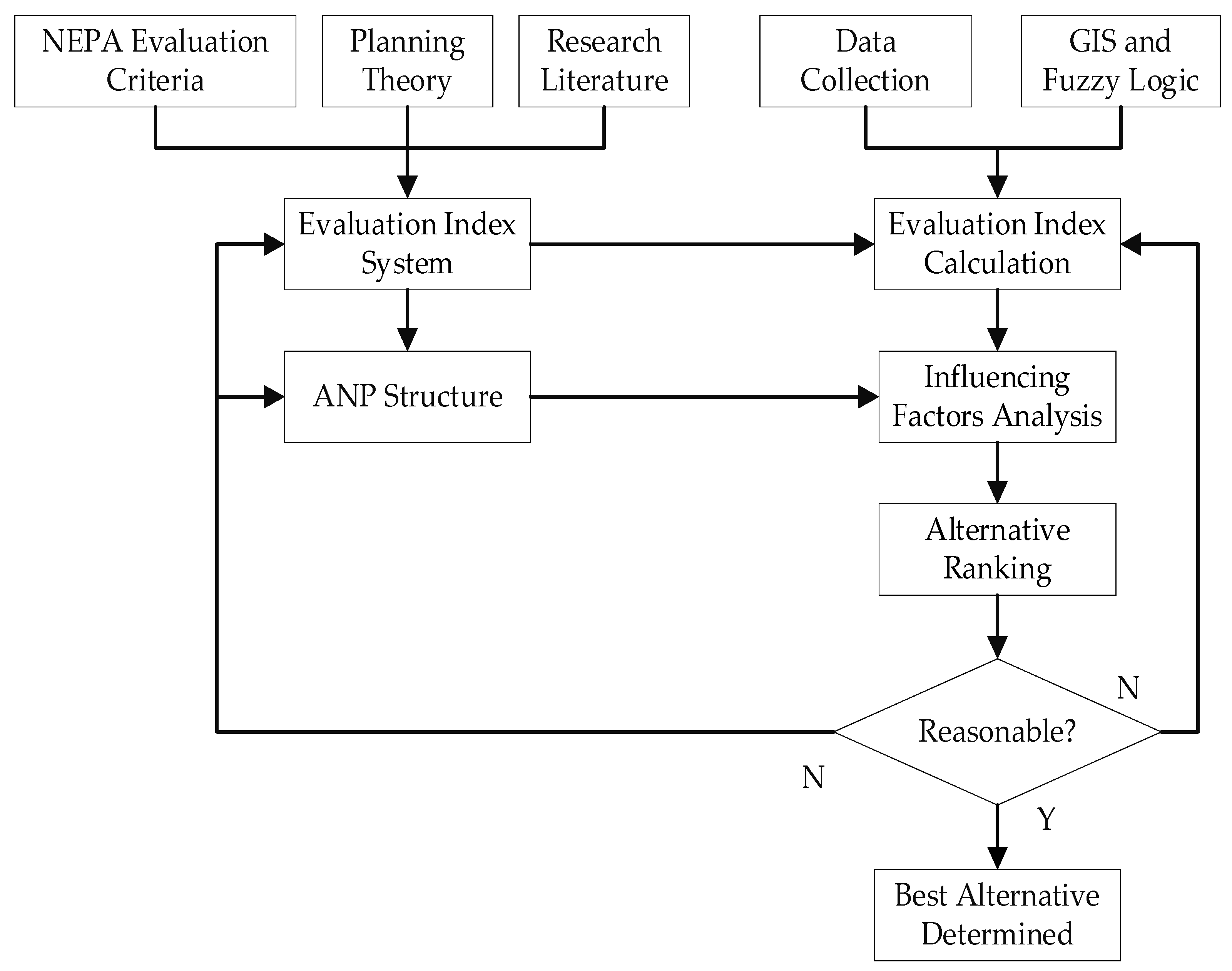
3.3. Comprehensive Evaluation Method of GIS-ANP

ANP was proposed on the basis of AHP [16]; its basic function is to compare the constituent factors and factor groups of a system according to the criteria for each alternative, and then obtain the relative importance of constituent factors and factor groups to finally obtain the priority of alternatives after processing. The structure of ANP is shown in Figure 5 below.

ANP consists of three parts and the connecting lines represent the relationships between components of the model, including internal and external dependencies and feedback relationships.

(1)

Control Layer: This part includes the research target of the system and the criteria that affect the decision-making to achieve the target (the target is the final goal of the model, which is to obtain the ranking of planning alternatives). All criteria are considered to be independent of each other and only governed by the target, and the value of the constituent factor in ANP will change with the attribution criteria. The weight of each criterion in the Control Layer can be obtained by establishing a weighted matrix.

(2)

Network Layer: This part is composed of all the factor groups dominated by the Control Layer. The Network Layer is an interactive network structure, which reflects the relationships among the factors and among the factor groups in the network under the corresponding Target and Criteria. C_i in the Network Layer is the cluster which represents the constituent factor group, and $e_{ij}$ in each C_i is the node which represents the constituent factor.

(3)

Alternative Layer: This part consists of all alternatives involved in the system. The Alternative Layer will interact with the Network Layer and often participate in the calculation as a factor group in the Network Layer.

Because it allows the coexistence of qualitative and quantitative indicators, ANP is very suitable for complex systems with internal dependence and feedback. Compared with the AHP method, ANP is closer to real decision-making problems.

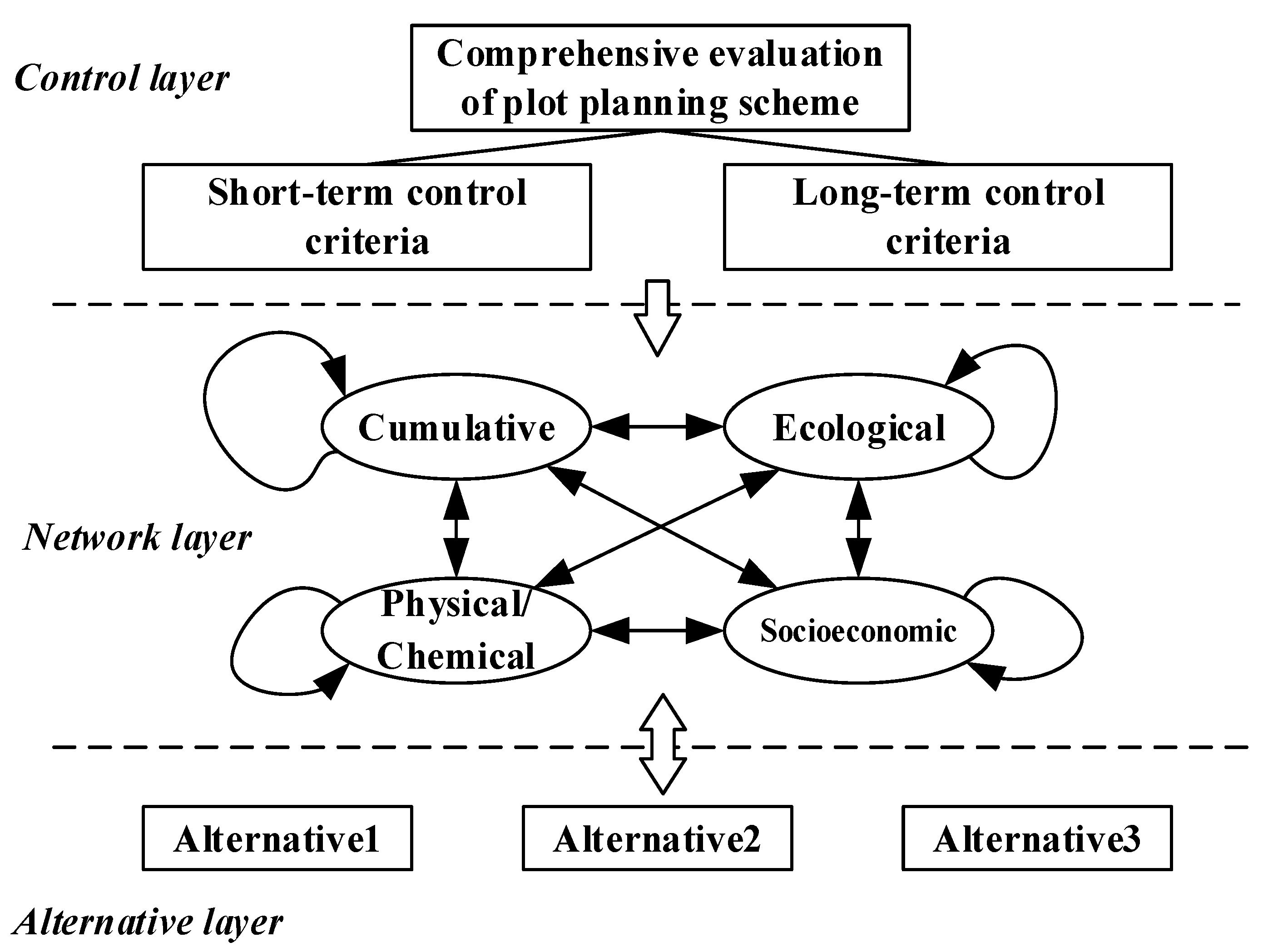
3.3.1. ANP Network Construction for the Case Study Area

The influencing factors of land use planning are divided into two parts. The first part is the control layer, including the general objectives and control criteria: in this study, short-term criteria focus on economic, transportation, and productivity improvement while long-term criteria focus on sustainable development. The second part is the network layer, which is a network structure composed of interacting influencing factors. The third layer of the network consists of alternatives that will interact with the network layer. The ANP model for land use planning evaluation is shown in Figure 6.

3.3.2. Indicator Standardization

Since the index set (see Table 2) includes two kinds of factors in different directions, benefit (positive) and cost (negative), the quantitative meaning of each index is also different. Therefore, it is necessary to standardize the original index value when constructing the comparison matrix.

Let $x_j\left(i\right)$ (i = 1,2, … m; j = 1,2, … n) be the j-th factor value of the i-th factor group;

If it is a positive indicator, the normalized value is:

$$x_j^{,}\left(i\right)=\frac{x_j\left(i\right)-{min}_i{h}_j\left(i\right)}{{max}_i{h}_j\left(i\right)-{min}_i{h}_j\left(i\right)}$$

(7)

If it is a negative indicator, the normalized value is:

$$x_j^{,}\left(i\right)=\frac{{max}_i{h}_j\left(i\right)-x_j\left(i\right)}{{max}_i{h}_j\left(i\right)-{min}_i{h}_j\left(i\right)}$$

(8)

3.3.3. Determination of Relative Importance Weights

Unweighted Hypermatrix Construction

The function of the unweighted hypermatrix is to find the relative importance of influencing factors within the clusters in each alternative. The unweighted hypermatrix was constructed according to the following steps.

(1) For every alternative, influencing factors in each cluster C_i were compared in pairs to obtain the judgment matrix $A_i$ of factor importance.

$$A_i=\left(a_{kj}\right)$$

$A_i$ can also be expressed as:

Ci	$e_{i1}{ e_{i2} \dots e}_{i{n}_i}$
$$\begin{gathered} e_{i1} \\ {e}_{i2} \\ \dots \\ {e}_{i{n}_i} \end{gathered}$$	$$\begin{gathered} a_{11}{ a_{12} \dots a}_{1n_i} \\ {a}_{21}{ a_{22} \dots a}_{2n_i} \\ \hspace{1em}\hspace{1em}\hspace{1em}\dots \\ {a}_{n_{i}1}{ a_{n_{i}2} \dots a}_{n_i{n}_i} \end{gathered}$$

Since there are five factor groups (Alternatives (A), Cumulative (C), Ecological (E), Physical/Chemical (P), and Socioeconomic (S)) for each alternative (see Table 1), five judgment matrices were created for every alternative in this step.

(2) Based on the judgment matrix, the relative importance weight $W_{i_k}$ of each influencing factor was calculated using the Geometric Mean method (Equation (9)) in the unit of factor group. The Geometric Mean method refers to a central tendency measure that evaluates the average of a series by multiplying all the numbers and then finding the root of the product.

$$W_{i_k}={\left(\prod _{j=1}^{n_i}{a}_{kj}\right)}^{1/n_i}, k=1, 2,\dots ,n_i$$

(9)

where n is the number of factors while $n_i$ is the i-th factor in the factor group C_i, and the definition of $a_{kj}$ is the same as above.

(3) Normalizing $W_{i_k}$ to make the relative importance weight $W_{i_k}$ comparable:

$$w_{i_k}^0{=W}_{i_k}/\sum _{k=1}^{n_i}{W}_{i_k}$$

(10)

where $w_{i_k}^0$ is the normalized relative importance weight of each influencing factor.

(4) Finally, all $w_{i_k}^0$ in factor groups were summarized and arranged based on the corresponding relationship of clusters to obtain the unweighted hypermatrix $W_s$.

$$W_s=\begin{array}{cc}W& \begin{array}{ccc}\begin{array}{cc}{C}_1\hspace{1em}& \hspace{1em}{C}_2\end{array}& \dots & C_N\\ \begin{array}{cc}{e}_{11}\dots e_{{1n}_1}& e_{21}\dots e_{2n_2}\end{array}& \dots & e_{N1}\dots e_{N{n}_N}\end{array}\\ \begin{array}{cc}{C}_1& \begin{array}{c}{e}_{11}\\ ⋮\\ e_{{1n}_1}\end{array}\\ C_2& \begin{array}{c}{e}_{21}\\ ⋮\\ e_{{2n}_2}\end{array}\\ \begin{array}{c}⋮\\ C_N\end{array}& \begin{array}{c}⋮\\ \begin{array}{c}{e}_{N1}\\ ⋮\\ e_{{Nn}_N}\end{array}\end{array}\end{array}& \left[\begin{array}{c}\hspace{1em}\hspace{1em}\hspace{1em}\hspace{1em}\hspace{1em}\hspace{1em}\hspace{1em}\hspace{1em}\hspace{1em}\hspace{1em}\hspace{1em}\hspace{1em}\hspace{1em}\hspace{1em}\hspace{1em}.\\ \begin{array}{c}\hspace{1em}{W}_{11}\hspace{1em}\hspace{1em}{W}_{12}\hspace{1em}\hspace{1em}\dots \hspace{1em}\hspace{1em}{W}_{1N}\hspace{1em}\\ \\ \\ \hspace{1em}{W}_{21}\hspace{1em}\hspace{1em}{W}_{22}\hspace{1em}\hspace{1em}\dots \hspace{1em}\hspace{1em}{W}_{2N}\hspace{1em}\\ \\ \dots \\ \\ \hspace{1em}{W}_{N1}\hspace{1em}\hspace{1em}{W}_{N2}\hspace{1em}\hspace{1em}\dots \hspace{1em}\hspace{1em}{W}_{NN}\hspace{1em}\\ \end{array}\\ \hspace{1em}\hspace{1em}\hspace{1em}\hspace{1em}.\end{array}\right]\end{array}$$

(11)

Weighted Matrix Construction

After the unweighted hypermatrices were constructed, the weighted matrix was then constructed to find the relative importance weight among influencing factor groups.

$$A_s=\left[\begin{array}{cc}\begin{array}{cc}{a}_{11}& a_{12}\\ a_{21}& a_{22}\end{array}& \begin{array}{cc}\cdots & a_{1N}\\ \cdots & a_{2N}\end{array}\\ \begin{array}{cc}⋮& ⋮\\ a_{N1}& a_{N2}\end{array}& \begin{array}{cc}⋮& ⋮\\ \cdots & a_{NN}\end{array}\end{array}\right]$$

(12)

Since the weighted matrix $A_s$ only represents the normalized relative importance weight among influencing factor groups, two weighted matrices $A_s$ were constructed for both short-term and long-term criteria in this project.

Weighted Hypermatrix Construction

Based on the two kinds of matrices above, the weighted hypermatrix $W_s^w$ that represents the overall relative importance weight of alternatives was constructed by multiplying the unweighted hypermatrix $W_s$ and the weighted matrix $A_s$.

$$W_s^w=A_s{W}_s$$

(13)

Because there are many relationships such as feedback and dependence between influencing factors, the importance order of factors cannot be obtained through direct comparison. Therefore, it is necessary to repeatedly iterate and stabilize the weighted hypermatrix $W_s^w$ to obtain its most stable state: the limit super matrix $w_s^l$ (14):

$$w_s^l=\underset{m\to \infty }{\lim }{{(W}_s^w)}^m$$

(14)

3.3.4. Alternatives Ranking

Values of these constructed limit super matrices $w_s^l$ were compared to obtain the ranking of each proposed planning alternative.

4. GIS-ANP Comprehensive Evaluation Results

According to the above GIS-ANP comprehensive evaluation method and the final index value, all evaluation indexes under short-term and long-term criteria were calculated. The Super Decisions software was used for the ANP calculation. The ANP structure has been iterated and revised several times to acquire the optimal results. There are many design data and large tables in the whole process, which are not all listed here, but can be obtained from the lead author. The results contain three parts: results of influencing factors analysis, main influencing factors of alternatives, and finally, the ranking of the planning alternatives.

4.1. Results of Influencing Factors Analysis

Table 3. Cluster matrix view of the SD mod for short-term and long-term decision.

	Alternatives (A)		Cumulative (C)		Ecological (E)		Physical/ Chemical (P)		Socioeconomic (S)
	S-T	L-T	S-T	L-T	S-T	L-T	S-T	L-T	S-T	L-T
Alternatives (A)	/	/	0.1356	0.0000	0.0000	0.6270	0.0000	0.6254	0.0959	0.6274
Cumulative (C)	0.1026	0.0972	0.1143	0.0972	0.1045	0.0503	0.1210	0.0762	0.1717	0.0769
Ecological (E)	0.4621	0.4018	0.4699	0.4018	0.4717	0.1237	0.5385	0.1441	0.4102	0.1258
Physical/Chemical (P)	0.1344	0.1640	0.0000	0.1640	0.1498	0.1237	0.1210	0.1005	0.0831	0.0548
Socioeconomic (S)	0.3008	0.3370	0.2801	0.3370	0.2741	0.0754	0.2196	0.0538	0.2392	0.1152
Overall	1.0000	1.0000	1.0000	1.0000	1.0000	1.0000	1.0000	1.0000	1.0000	1.0000

below shows the ANP Super Decisions Module (SD mod), a group matrix of the Super Decisions software which shows the overall relationship among all influencing factor groups. All factors were considered affecting each other and themselves.

Values for each column in the table show the overall amount of influence among all factors to another one and the sum is 1. The values in the table represent the proportion of each factor’s influence in the total amount, and the bold number marks the highest proportion of influence among all influences in this study. For instance, in the short-term (S-T), Cumulative (C) has an influence of 0.1143 to itself, and Ecological (E) has an influence of 0.4699 to Cumulative (C); this indicates that when evaluating all the influencing factors of Cumulative (C), Ecological (E) has the highest influence, about four times greater than Cumulative (C) itself. As a result, in the short-term, Ecological (E) is the most influential factor for Cumulative (C) among all factors taken in the research. As for values of 0.0000, they represent the minimum and most insignificant influence (less than 0.00005) among all factors, indicating that the factor is the least to be considered when measuring its influence.

• Short-term

It can be seen from Table 3 that the most important influencing factor group in the short-term is Ecological (E). It has the highest proportion (above 40%) of influence among all factor groups: 46.21% to Alternatives (A), 46.99% to Cumulative (C), 47.17% to Ecological (E), 53.85% to Physical/Chemical (P), and 41.02% to Socioeconomic (S).

On the other hand, however, there are factor groups that have little influence among all groups, like Physical/Chemical (P) and Cumulative (C), which have only 13.44% and 10.26% to Alternatives (A), less than 0.001% and 11.43% to Cumulative (C), 14.98% and 10.45% to Ecological (E), 12.10% to Physical/Chemical (P), and 8.31% and 17.17% to Socioeconomic (S).

• Long-term

The results are not the same when it comes to the long-term effect. Although Ecological (E) still has the highest proportion of influence (40.18%) to factor groups Alternatives (A) and Cumulative (C), factor group Alternatives (A) has the highest proportion of influence to three groups (62.70% to Ecological (E), 62.54% to Physical/Chemical (P), and 62.74% to Socioeconomic (S)). However, it is worth noting that, as an important factor in evaluating long-term impacts, the influence of Cumulative (C) is exceptionally low (all less than 10%) compared to all other factors for this location.

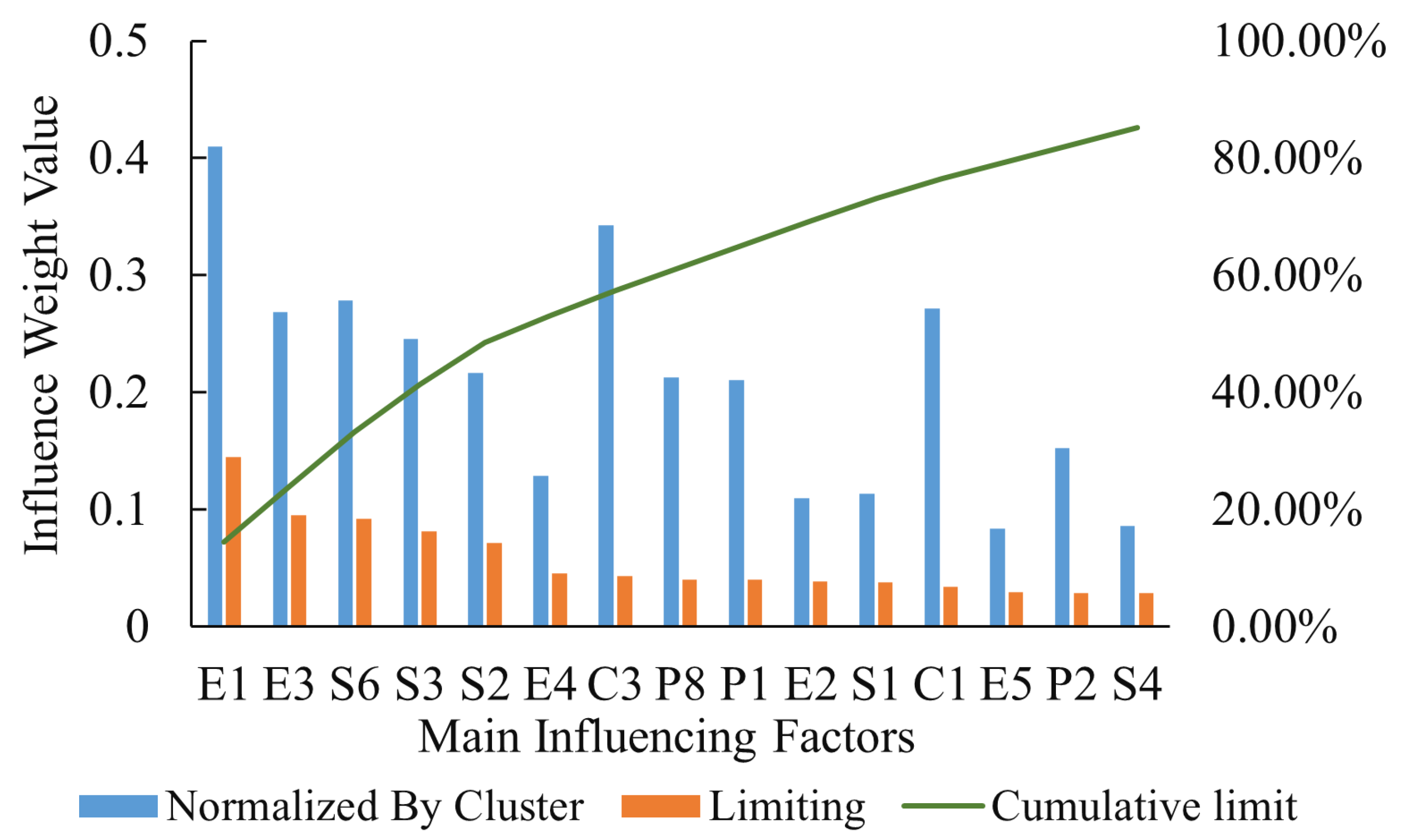
4.2. Main Influencing Factors for Land Use Planning Decision

4.2.1. Influencing Factor Groups for Planning Alternative

Under the short-term and long-term decision criteria, the weight distribution of the four influencing groups to Alternatives is shown in Figure 7 below. It can be seen from the figure that the weight ranking results of the four groups are the same regardless of long-term or short-term. Ecological (E) is the most important influencing factor group (more than 40%), followed by Socioeconomic factors (above 30%), Physical and Chemical factors (10–17%), and Cumulative related factors (10%).

One thing worth noting is that, in the long-term decision, the weight proportion of Socioeconomic and Physical/Chemical increased, albeit a little, indicating their greater importance in planning with long-term goals than short-term ones.

4.2.2. Main Influencing Factors for Planning Alternatives

According to all calculated factor weights (priorities) of ANP, the influencing factors of short-term and long-term decisions, excluding the weight proportions of the selection alternative itself, are shown in Figure 8 and Figure 9. In these figures, the blue bar (Normalized By Cluster) represents the importance of the influencing factor in its group, whereas the brown bar (Limiting) represents the weighted importance of that factor overall. For instance, factor C3 has a factor weight normalized by cluster of 36% (blue bar value), which means it has a 36% influence in its Cluster Cumulative (C); on the other hand, C3 has a limiting factor weight of 16.88% (brown bar value), which means it has a 16.88% influence overall.

As can be seen from Figure 8, the first three indicators (limiting factors) that affect short-term decisions are C3 (16.88%), C2 (12.75%), and C1 (9.16%), followed by E5 (8.16%) and E4 (7.96%). Further, from the perspective of long-term development, the most important factors in planning are E1(14.49%), E3 (9.50%), S6 (9.20%), S3 (8.13%), and S2 (7.16%) (Figure 9).

4.3. Planning Alternatives Ranking

Based on the above results of influencing factors, alternatives rankings were calculated. For the two criteria of short-term environmental/economic impact and long-term sustainable development of the control layer, the overall weight values and ranking of short-term and long-term alternatives calculated by ANP are shown in

Table 4. Alternative Rankings under the “short-term interest” control criteria.

Alternatives	Total	Normal	Ranking
A1	0.0305	0.3681	2
A2	0.0316	0.3816	1
A3	0.0208	0.2503	3

and

Table 5. Alternative Rankings under the “long-term development” control criteria.

Alternatives	Total	Normal	Ranking
A1	0.1451	0.3401	2
A2	0.2568	0.6020	1
A3	0.0247	0.0579	3

respectively. “Total” is the relative importance weight calculated by the software, “Normal” is the normalized weight, and “Ranking” is the total ranking of the alternative.

According to the evaluation results in Table 3, the normalized relative importance weight of A2 is 0.3816 while that of A1 is 0.3681. A2 and A1 rank first and second respectively and the difference between them is small, but there is a significant difference compared to A3 (0.2503), which is in last place. The results indicate that on the premise of not violating the environmental protection rules, there is little difference between alternative A1 and A2 considering the short-term interests, but both are better than A3.

However, from the perspective of long-term environmental protection and sustainable development, the normalized relative importance weight of A2 (0.6020) is far better than that of A1 (0.3401), as shown in Table 4. Similarly like the short-term, A1 and A2 are also better than A3. Therefore, it is not recommended to maintain the plot in its original state (A3), neither in the short-term nor long-term.

5. Discussion

5.1. Findings and Implications

(1)

Relationships among influencing factors

Through the ANP network, this research has revealed relationships among influencing factors. The greatest impact among factor groups in the short-term is the Ecological (E) factor group, which means that, regardless of which alternative is selected, changes in ecological factors caused by the implementation of a planning alternative may also cause significant changes in other factors at the same time. For example, during construction, factors in the Ecological (E) group (like the change of habitat on site) may lead to changes in surface water runoff (Physical/Chemical) or changes in city traffic (Socioeconomic), far more than other factor groups.

These results suggest that planners in this case should pay more attention to ecological related factors than any other and need to fully consider the potential impact on all aspects of the region. This aligns with the findings of other studies that demonstrated that influencing factors involved interact with each other [30].

As for long-term, the choice of Alternative (A) will have a more profound and lasting impact on aspects of Ecological, Physical/Chemical, and Socioeconomic systems. This is not surprising, as the impact of different planning alternatives is comprehensive and sustained. Therefore, it is necessary to regularly monitor planned land use, especially for long-term impacts, which has been discussed by others [31]. At the same time, factor group Cumulative (C) has an exceptionally low influence for the study area, perhaps because there are not many cumulative impacts associated with at this location or may also because the cumulative influencing factors selected in this study are not closely related to the area.

The long-term results indicate the need for planners to be aware of the profound and lasting impacts on the ecological and socio-economic conditions of the area that their decisions may have, even if it is not obvious in the early stages of planning implementation [32]. Land use alternatives may not necessarily have a significant effect on sustainable development of an area [33].

It is not surprising that the influence weight priorities of factors in the Physical/Chemical factor group are not high because some factors in this group are temporary construction-related impacts. In addition, due to the small plot area size, impacts to flash flooding and air quality are limited. This finding suggests that not all indicators in the suggested evaluation index system are worth considering for some planning alternatives, because their changes will have an insignificant influence on other factors. Therefore, while considering the evaluation indicators involved in the land use planning, it is necessary to take the local situation into consideration, rather than relying solely on a general and common evaluation index system, as shown in another case study [34].

(2)

Influencing factors and alternative

The results of this study have revealed that, regardless of short-term or long-term considerations, the most important factors that will influence the choice of the best land-use alternative are the Ecological factors, followed by Socioeconomic factors, Physical/Chemical, and finally, Cumulative related factors. As for the single factor, the first three indicators (limiting factors) that affect short-term decisions are degradation of Hardee Creek (C3), violation of Tar River TMDL (C2), and future development patterns (C1). Therefore, a primary consideration for planning of this area is not to erode the river channel and pollute the downstream water body, and at the same time it is hoped to be consistent with the future development direction of the city. In the long-term, given the most important factors detailed previously, particular consideration should be given to the impact of the project on water and soil conservation, the change in traffic conditions, the cost of land acquisition, and the impact on citizens’ property after completion.

These results align with those of others [35] indicating that planners need to be aware that to achieve long-term goals, the influencing factors they should focus on may not necessarily be consistent with those of short-term goals. As a result, targeted plans need to be developed for different planning purposes.

Indeed, when considering the selection of planning alternatives, long-term impacts are likely to be more important than the short-term ones. Therefore, it will be of great benefit if planners can include predictions or calculations of potential future development trends of the region during the planning alternative design [36]. With the passage of time, while the plot development brings social effects, it also increases the physical and chemical changes of the plot and its adjacent areas, and over development may eventually lead to irreversible situations.

(3)

Alternative ranking

According to the GIS-ANP network analysis results, Alternative 2 (Low Density Residential) is the best planning alternative for this location, followed by Alternative 1 (High Density Residential and Commercial), with Alternative 3 (No Action, Remained Residential and Agricultural) ranking last. Although in the short term, there is not a significant difference between the impacts of low density residential and that of high density residential and commercial, impacts of low density residential is better in the long run considering sustainable development. This points up the need to consider the applicability of alternatives under different evaluation criteria (long-term and short-term criteria in this study). There are significant differences in the advantages and applicable conditions of each alternative as they will have various effects at different time scales [37].

5.2. Study Limitations

As with all studies of this type, there are several limitations. First, only three alternatives were considered in this study. Although each represents a different situation, there is still a significant similarity between them, because they all include residential land use. This similarity may result in smaller differences in the final rankings, as we can see from Table 4 (values of A2 and A1 are very close). Additionally, the quantity of three alternatives also has limited ability to reflect the selecting and discriminating power of the method.

Second, although the evaluation index system used in this study was established based on many references found in planning theory, NEPA evaluation criteria, and related literature, there is much opportunity for it to be optimized and improved. The background references provide common and general planning indicators, without referring to specific environmental or social conditions of the study location.

Further, in this study, GIS was used to determine the quantitative index values, but the GIS data acquired for this study were not always at the appropriate scale. The small size of this study area limits the availability of detailed socioeconomic and demographic data. The study area and surrounding properties represent an area smaller than a census block, the smallest available unit for which demographic and economic data are published in the American Community Survey. The information for Pitt County and the City of Greenville was used as representative for the area because this is the best available information at this scale. Using a survey instrument in the immediate area would provide a more accurate representation of the demographics and economic characteristics of the study area but this was beyond the scope of this study.

Finally, there are limitations to the determination of qualitative and final index values, since the task of determining these values was conducted by graduate students at East Carolina University, as mentioned before. Their knowledge and abilities in planning may not be as refined as experts in the field, which may cause flaws in the value determination. At the same time, using experts to evaluate all index values is a key component of the overall method. Although GIS is used to assist in determining quantitative indicator values, the process of value determination still depends on the knowledge and experience of experts in the relevant fields of planning and geography, as some indicators are directly valued by experts. Therefore, ensuring the qualification of the experts involved in the research is also one of the main challenges in using this method. Furthermore, it is important to note that the calculation results also have a certain degree of subjectivity, thus affecting the precision of the results, but not their utility or importance.

5.3. Future Work

The methodology and results of this project provide a solid foundation for future research. In addition to focusing on overcoming the limitations mentioned above, testing of the methods at different locations with different social and environmental contexts will help to refine the input data and the models used.

Further, some indicators such as Ecosystem Services [38], Urban Resilience [39], and overtourism [40] are increasingly seen to be important considerations in evaluating the impacts of various development alternatives and thus in evaluating urban or land planning. Therefore, future research needs to include these indicators (and others as appropriate) in evaluation systems, to further increase the objectivity of analysis results.

6. Conclusions

Land use planning is not a simple real-estate project; it is related to the overall urban development pattern, as well as economic, social and natural environment changes. Therefore, a method that provides a comprehensive evaluation result is necessary. In this paper, GIS spatial measurement is adopted to obtain objective index data of influencing factors, combined with an ANP analysis which takes both qualitative and quantitative factor groups and factors into consideration, to evaluate land use planning alternatives comprehensively. This study illustrates how the GIS-ANP method can combine qualitative and quantitative factors involved in land use planning for a comprehensive analysis, thus further revealing the relationships between influencing factors and planning alternatives, allowing for determination of the most suitable land use alternative. As a comprehensive method that intersects system science and GIS, the evaluation result is more objective, and the decision-making suggestions are also of strong geographical relevance. Therefore, its application in the field of land use planning alternative evaluation or other planning related evaluation holds great promise. However, for the methods proposed, what is critical is that the most reasonable evaluation results can be obtained only by putting forward an evaluation index system of planning, and correctly measuring all index values. This prerequisite requirement may become one of the obstacles to the wider application of the methods proposed in this paper.

References

1. Lichfield, N.; Kettle, P.; Whitbread, M. Evaluation in the Planning Process, 1st ed.; Pergamon Press: Oxford, UK, 1975. [Google Scholar]
2. Chabot, M.; Duhaime, G. Land-use planning and participation: The case of inuit public housing (nunavik, canada). Habitat Int. 1998, 22, 429–447. [Google Scholar] [CrossRef]
3. Berke, P.R.; Conroy, M.M. Are we planning for sustainable development? J. Am. Plan. Assoc. 2000, 66, 21–33. [Google Scholar] [CrossRef]
4. Morris, M. Measuring the Condition of the World’s Poor: The Physical Quality of Life Index, 42nd ed.; Pergamon Press for the Overseas Development Council: Ottawa, ON, Canada, 1979; Available online: https://unesdoc.unesco.org/ark:/48223/pf0000037164 (accessed on 20 December 2022).
5. Morris, M.D. Measuring the Condition of the World’s Poor: The Physical Quality of Life Index; The Population and Development Council: New York, NY, USA, 1981; Available online: https://www.jstor.org/stable/1972820; (accessed on 20 December 2022). [Google Scholar] [CrossRef]
6. Wackernagel, M.; Rees, W. Our Ecological Footprint: Reducing Human Impact on the Earth; New Society Publishers: Gabriola Island, BC, Canada, 1998. [Google Scholar]
7. Prescott-Allen, R. Barometer of Sustainability: Measuring and Communicating Wellbeing and Sustainable Development; IUCN: Gland, Switzerland, 1997. [Google Scholar]
8. Esty, D.C.; Levy, M.; Srebotnjak, T.; De Sherbinin, A. Environmental sustainability index: Benchmarking national environmental stewardship. New Haven Yale Cent. Environ. Law Policy 2005, 47, 60. [Google Scholar]
9. Van de Kerk, G.; Manuel, A.R. A comprehensive index for a sustainable society: The SSI—The sustainable society index. Ecol. Econ. 2008, 66, 228–242. [Google Scholar] [CrossRef]
10. Usubiaga-Liano, A.; Ekins, P. Monitoring the environmental sustainability of countries through the strong environmental sustainability index. Ecol. Indic. 2021, 132, 108281. [Google Scholar] [CrossRef]
11. Ali-Toudert, F.; Ji, L.; Fährmann, L.; Czempik, S. Comprehensive assessment method for sustainable urban development (CAMSUD)—A new multi-criteria system for planning, evaluation and decision-making. Prog. Plan. 2020, 140, 100430. [Google Scholar] [CrossRef]
12. Li, Q.; Roy, M.; Mostafavi, A.; Berke, P. A plan evaluation framework for examining stakeholder policy preferences in resilience planning and management of urban systems. Environ. Sci. Policy 2021, 124, 125–134. [Google Scholar] [CrossRef]
13. Domingo, D.; Palka, G.; Hersperger, A.M. Effect of zoning plans on urban land-use change: A multi-scenario simulation for supporting sustainable urban growth. Sustain. Cities Soc. 2021, 69, 102833. [Google Scholar] [CrossRef]
14. Puchol-Salort, P.; O’Keeffe, J.; van Reeuwijk, M.; Mijic, A. An urban planning sustainability framework: Systems approach to blue green urban design. Sustain. Cities Soc. 2021, 66, 102677. [Google Scholar] [CrossRef]
15. Maurya, S.P.; Singh, P.K.; Ohri, A.; Singh, R. Identification of indicators for sustainable urban water development planning. Ecol. Indic. 2020, 108, 105691. [Google Scholar] [CrossRef]
16. Saaty, T.L. Time dependent decision-making; dynamic priorities in the AHP/ANP: Generalizing from points to functions and from real to complex variables. Math. Comput. Model. 2007, 46, 860–891. [Google Scholar] [CrossRef]
17. U.S. Census Bureau. Quick Facts Greenville, North Carolina. 2019. Available online: https://www.census.gov/quickfacts/greenvillecitynorthcarolina (accessed on 16 November 2020).
18. U.S. Census Bureau. Quick Facts Pitt County, North Carolina. 2019. Available online: https://www.census.gov/quickfacts/pittcountynorthcarolina (accessed on 16 November 2020).
19. Pitt County Board of Commissioners. Annual Capital Budgeting Workshop. 22 January 2018. Available online: https://www.pittcountync.gov/AgendaCenter/ViewFile/Minutes/_01222018-542 (accessed on 16 November 2020).
20. Greenville Planning and Zoning Commision. Agenda Planning and Zoning Commission. 18 August 2020. Available online: https://www.ci.greenville.tx.us/432/Planning-Zoning-Commission (accessed on 16 November 2020).
21. North Carolina Department of Environment and Natural Resources. Nutrient Sensitive Water Strategy. 2014. Available online: https://ncdenr.maps.arcgis.com/apps/webappviewer/index.html?id=6e125ad7628f494694e259c80dd64265 (accessed on 16 November 2020).
22. U.S. Environmental Protection Agency. TMDL Case Study: Tar-Pamilco Basin, North Carolina. 1993. Available online: https://nepis.epa.gov/Exe/ZyNET.exe/20004PRE.TXT?ZyActionD=ZyDocument&Client=EPA&Index=1991+Thru+1994&Docs=&Query=&Time=&EndTime=&SearchMethod=1&TocRestrict=n&Toc=&TocEntry=&QField=&QFieldYear=&QFieldMonth=&QFieldDay=&IntQFieldOp=0&ExtQFieldOp=0&XmlQuery=&File=D%3A%5Czyfiles%5CIndex%20Data%5C91thru94%5CTxt%5C00000008%5C20004PRE.txt&User=ANONYMOUS&Password=anonymous&SortMethod=h%7C-&MaximumDocuments=1&FuzzyDe-gree=0&ImageQuality=r75g8/r75g8/x150y150g16/i425&Display=hpfr&DefSeekPage=x&SearchBack=ZyActionL&Back=ZyActionS&BackDesc=Results%20page&MaximumPages=1&ZyEntry=1&SeekPage=x&ZyPURL (accessed on 16 November 2020).
23. Schoonover, J.E.; Lockaby, B.G. Land cover impacts on stream nutrients and fecal coliform in the lower piedmont of west georgia. J. Hydrol. 2006, 331, 371–382. [Google Scholar] [CrossRef]
24. Chithra, S.V.; Nair, M.H.; Amarnath, A.; Anjana, N.S. Impacts of impervious surfaces on the environment. Int. J. Eng. Sci. Invent. 2015, 4, 27–31. [Google Scholar]
25. North Carolina Planning and Zoning Commission. Agenda: City of Greenville. 2020. Available online: https://d3n9y02raazwpg.cloudfront.net/greenville/a8db001e-5363-11eb-920e-0050569183fa-fa05477a-065e-4ca2-a3ab-6395dc97ae5a-1623455699.pdf (accessed on 16 November 2020).
26. Prasannakumar, V.; Vijith, H.; Abinod, S.; Geetha, N. Estimation of soil erosion risk within a small mountainous sub-watershed in kerala, india, using revised universal soil loss equation (RUSLE) and geo-information technology. Geosci. Front. 2012, 3, 209–215. [Google Scholar] [CrossRef] [Green Version]
27. Xia, S.; Gao, W.; Cheng, J.; Wang, M.; Cheng, G. Calculation method of peak flow in urban rivers based on rainfall process theory and its application. China Water Wastewater 2017, 33, 43–47. [Google Scholar]
28. Le, N.D.; Zidek, J.V. Statistical Analysis of Environmental Space-Time Processes, 1st ed.; Springer Science + Business Media: New York, NY, USA, 2006; Available online: https://link.springer.com/book/10.1007/0-387-35429-8 (accessed on 28 December 2022).
29. Liao, Y.; Sun, X.; Jia, L.; Dong, H.; Zhang, Q. Evaluating traffic status of urban expressway in beijing based on road vehicle capacity. Logist. Technol. 2012, 31, 87–89. [Google Scholar]
30. Marull, J.; Padró, R.; La Rota-Aguilera, M.J.; Pino, J.; Giocoli, A.; Cirera, J.; Velasco-Fernández, R. Modelling land use planning: Socioecological integrated analysis of metropolitan green infrastructures. Land Use Policy 2023, 126, 106558. [Google Scholar] [CrossRef]
31. Wiwoho, B.S.; Phinn, S.; McIntyre, N. Characterizing watersheds to support land-use planning in indonesia: A case study of brantas tropical watershed. Ecohydrol. Hydrobiol. 2023, in press. [CrossRef]
32. Duggan, I.C. Urban planning provides potential for lake restoration through catchment re-vegetation. Urban For. Urban Green. 2012, 11, 95–99. [Google Scholar] [CrossRef]
33. Kosow, H.; Wassermann, S.; Bartke, S.; Goede, P.; Grimski, D.; Imbert, I.; Protzer, J. Addressing goal conflicts: New policy mixes for commercial land use management. Land 2022, 11, 795. [Google Scholar] [CrossRef]
34. Öztürk, M.; Bolat, İ.; Gökyer, E. Land use suitability classification for the actual agricultural areas within the bartın stream watershed of turkey. Period. Eng. Nat. Sci. 2017, 5, 30–36. [Google Scholar] [CrossRef]
35. Metternicht, G. Land use planning. Glob. Land Outlook (Work. Pap.) 2017, 2, 25–31. [Google Scholar]
36. García-Ayllón, S. La manga case study: Consequences from short-term urban planning in a tourism mass destiny of the spanish mediterranean coast. Cities 2015, 43, 141–151. [Google Scholar] [CrossRef]
37. Zhang, Y.; Wang, M.; Zhang, D.; Lu, Z.; Bakhshipour, A.E.; Liu, M.; Tan, S.K. Multi-stage planning of LID-GREI urban drainage systems in response to land-use changes. Sci. Total Environ. 2023, 859, 160214. [Google Scholar] [CrossRef] [PubMed]
38. Zepp, H.; Inostroza, L. Who pays the bill? assessing ecosystem services losses in an urban planning context. Land 2021, 10, 369. [Google Scholar] [CrossRef]
39. Feng, X.; Xiu, C.; Li, J.; Zhong, Y. Measuring the evolution of urban resilience based on the Exposure–Connectedness–Potential (ECP) approach: A case study of shenyang city, china. Land 2021, 10, 1305. [Google Scholar] [CrossRef]
40. Buitrago, E.M.; Yñiguez, R. Measuring overtourism: A necessary tool for landscape planning. Land 2021, 10, 889. [Google Scholar] [CrossRef]
Figure 1. Map of the rezoning site location relative to the City of Greenville municipal boundaries. The locator map (top right) indicates Pitt County in the context of eastern North Carolina.
Land 12 01489 g001
Figure 2. Map of the soil types and the modeled flow direction for precipitation for the site. Flow direction arrows represent 75-foot cells across the study area. The elevation contours can be used to estimate groundwater head in surficial aquifers.
Land 12 01489 g002
Figure 3. Transportation in the Project Area.
Land 12 01489 g003
Figure 4. Workflow for research methodology.
Land 12 01489 g004
Figure 5. ANP structure.
Land 12 01489 g005
Figure 6. ANP network structure of land use planning evaluation.
Land 12 01489 g006
Figure 7. Priority of clusters for short-term and long-term decision.
Land 12 01489 g007
Figure 8. Priority of factor weight for short-term decision.
Land 12 01489 g008
Figure 9. Priority of factor weight for long-term decision.
Land 12 01489 g009