
The Relationship between Rural Spatial Form and Carbon Emission—A Case Study of Suburban Integrated Villages in Hunan Province, China

Abstract
:1. Introduction
2. Relevant Theoretical Background
2.1. Hierarchy of Spatial Form and Indicators
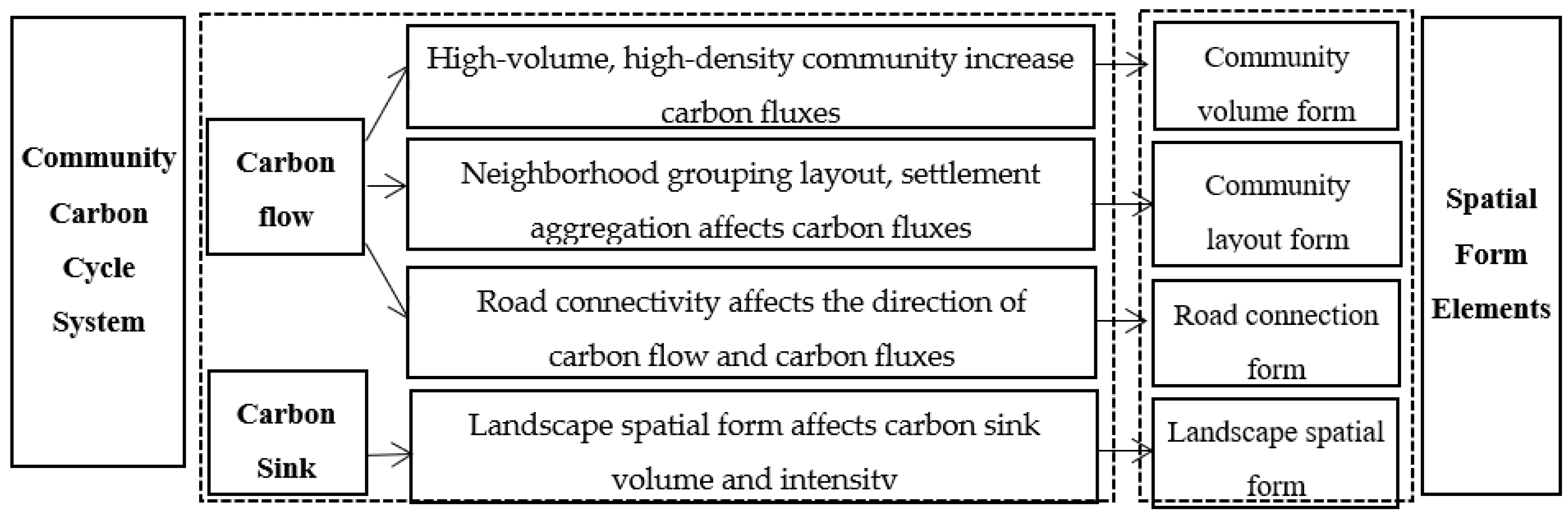
2.2. Correlation between Spatial Form and Carbon Emissions
- (1)
- The overall spacial form of rural communities, such as the total community area, building land area, building density, and other elements, affects the overall level of community carbon emissions in terms of total amount, increasing carbon fluxes [40].
- (2)
- Secondly, the spatial morphology of neighborhood building groups, such as the aggregation and connectivity of settlements, affects the carbon fluxes of the building system [26].
- (3)
- The spatial morphology of roads affects transport carbon input/output fluxes and carbon circulation intensity, as the distances of residences from work and public spaces significantly influences transport use and thus transport carbon fluxes [41].
3. Research Methods
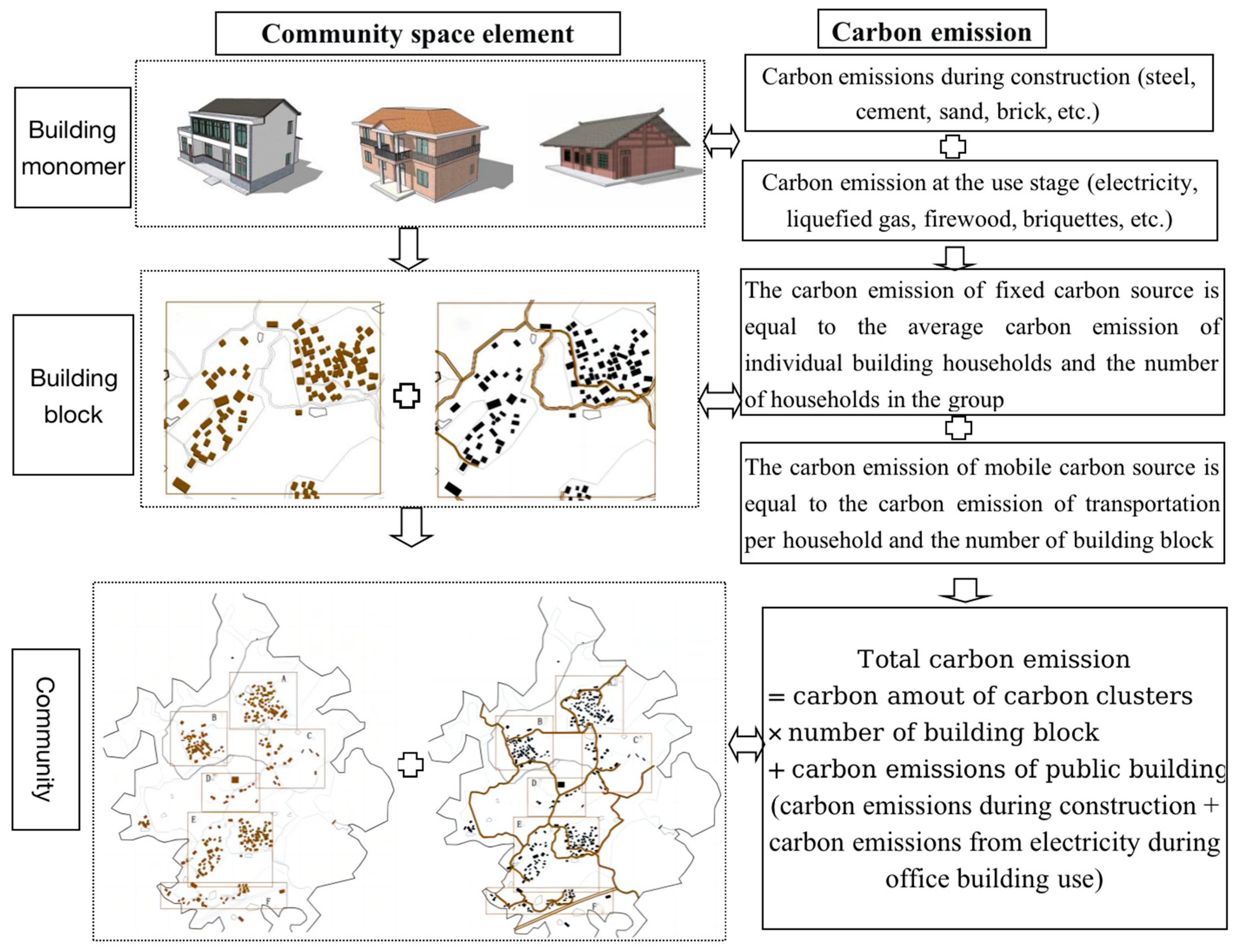
3.1. Measuring Carbon Emissions of the Rural Community
3.2. Quantification of Spatial Form Indicators
3.3. Correlation Analysis
- (1)
- Partial Correlation Analysis
- (2)
- Measuring the Contributions of Driving Factors
- (3)
- Regression Fitting
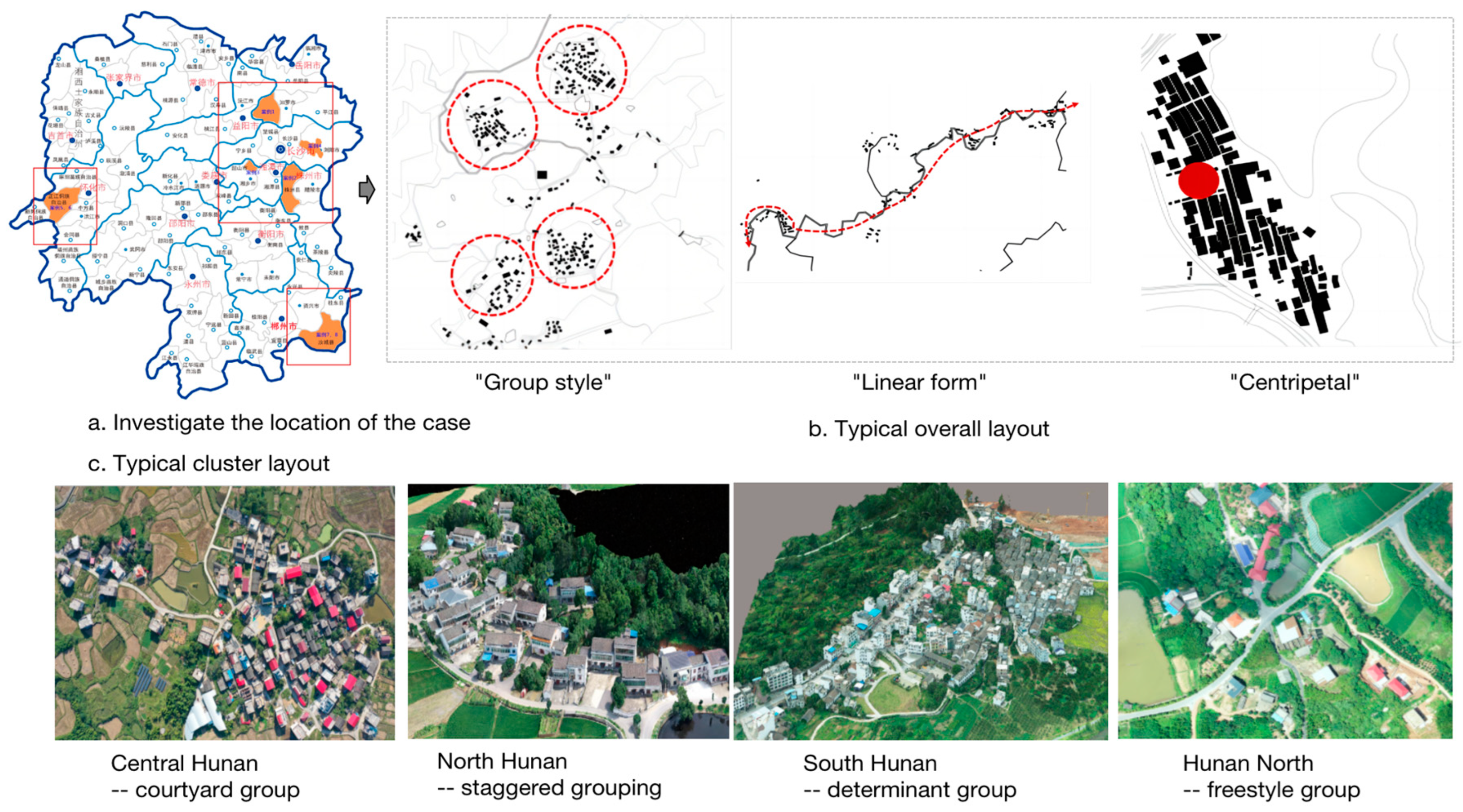
4. Results—The Case of Hunan’s Suburban Integrated Villages
4.1. Indicators of Spatial Form in the Case Villages
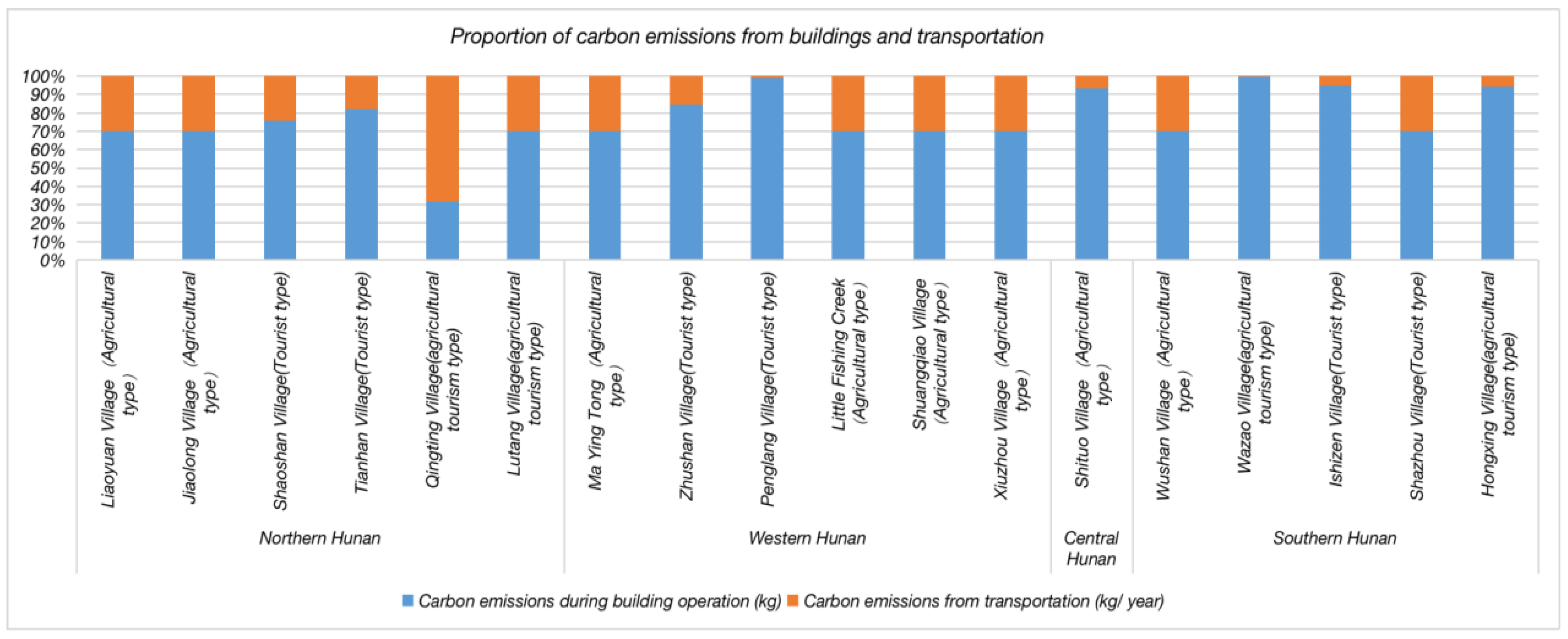
4.2. Identifying Carbon Emissions in the Sample Villages
4.2.1. Carbon Emissions from Buildings
- (1)
- Construction Phase Carbon Emissions

| Material Name | Use Parts | Usage | Unit | Obsolescence Rate | Carbon Emission Factor | Carbon Emissions | |
|---|---|---|---|---|---|---|---|
| Brick building | Clay bricks | Exterior wall, interior wall, footer, foundation | 151 | m3 | 5% | 323.4 kgCO2 e/m3 | 51,275.07 |
| Caliber galvanized steel pipe | Roof | 0.12 | t | 7% | 2190 kgCO2 e/t | 281.20 | |
| C30 concrete | Ring beam, floor slab, mat | 138.7 | m3 | 1.5% | 295 kgCO2 e/m3 | 44,153.21 | |
| Ordinary silicate cement | Masonry mortar, plastering mortar | 28.06 | t | 5% | 735 kgCO2 e/t | 20,173.55 | |
| Lime | Foundation bedding | 6.58 | t | 5% | 1190 kgCO2 e/t | 7659.44 | |
| Steel reinforcement | Ring beam, floor slab | 4.10 | t | 7% | 2310 kgCO2 e/t | 10,776.61 | |
| Gravel | Foundation bedding | 25.87 | t | 5% | 2.18 kgCO2 e/t | 59.22 | |
| Sand | Foundation, mortar | 112.28 | t | 5% | 2.51 kgCO2 e/t | 295.91 | |
| Aluminum–plastic co-extruded windows | Exterior Windows | 76.26 | m2 | 0 | 129 kgCO2 e/m2 | 9837.54 | |
| Tile | Exterior wall surface | 2.6 | t | 5% | 1.4 tCO2 e/t | 12,201.00 | |
| Coatings | Exterior wall surface | 1.29 | t | 5% | 1.2 tCO2 e/t | 764.40 | |
| Total carbon emissions (kg) | 157,477.14 | ||||||
| Type | Material Name | Use Parts | Usage | Unit | Obsolescence Rate | Carbon Emission Factor 1 | Carbon Emissions |
|---|---|---|---|---|---|---|---|
| Wood knot structure | Wood | Wall, roof frame | 100 | m3 | 10% | 283.55 kgCO2 e/m3 | 31,190.50 |
| Column cornerstone (column base) | Foundation bedding | 20 | m3 | 5% | 5.08 kgCO2 e/t | 1.60 | |
| Steel nails | Wood fixing | 10 | kg | 0 | 2375 kgCO2 e/t | 23.75 | |
| Green tiles | Roofing | 3200 | Block | 0 | 0.27 kgCO2 e/kg | 216 | |
| Total carbon emissions (kg) | 31,431.85 | ||||||
- (2)
- Carbon Emissions in the Use Phase
4.2.2. Transportation Carbon Emissions
4.2.3. Total Carbon Emissions of the Rural Community
4.3. Correlation between Spatial Form and Carbon Emissions
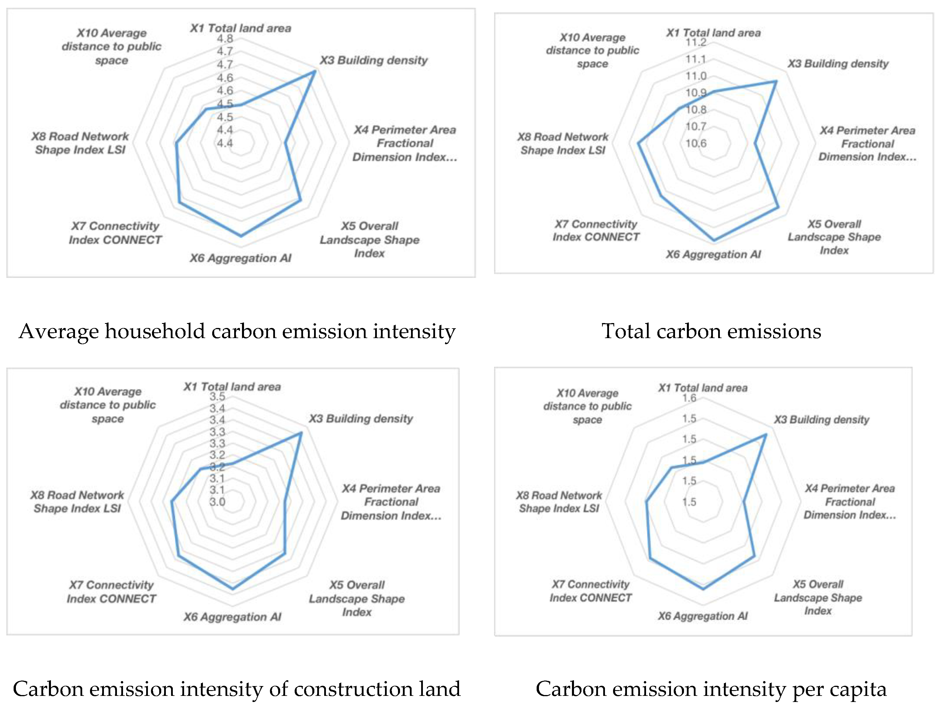
4.3.1. Correlation between Overall Community Spatial Patterns and Carbon Emissions
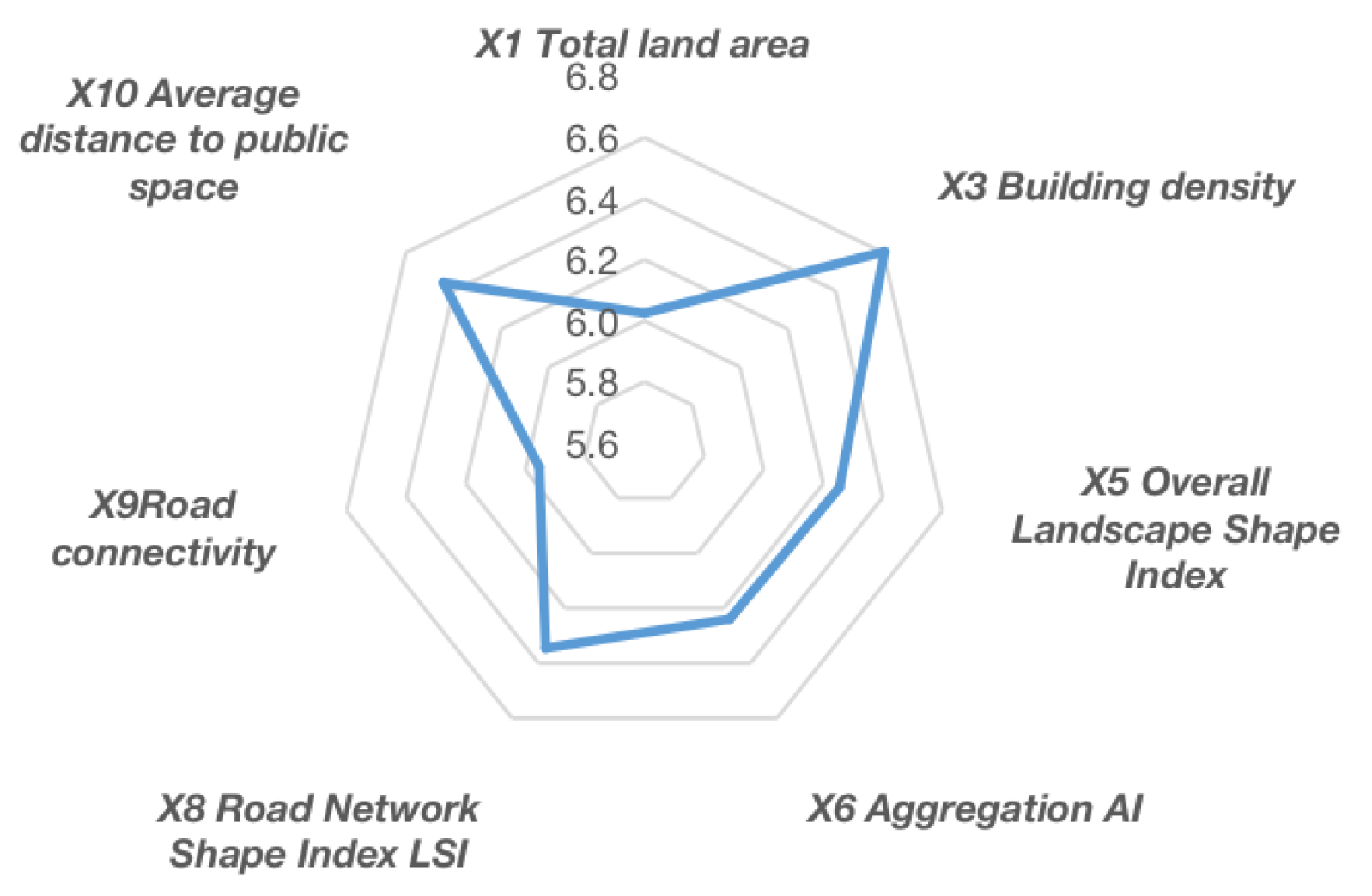
4.3.2. Relationship between Rural Community Spatial Form and Carbon Emissions from Transport
4.3.3. Relationship between the Spatial Form of Neighborhood Building Groups and Carbon Emissions
- (1)
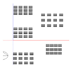
- Controlling the Density of Building Groups
- (2)
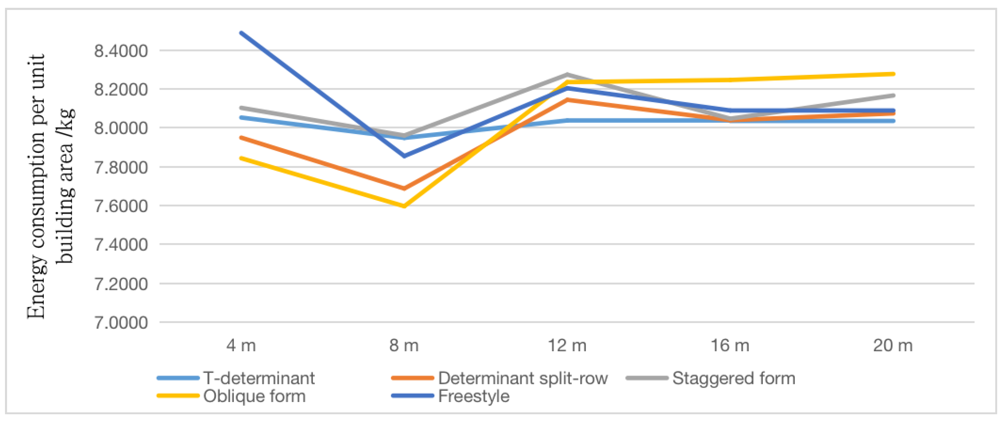
- Controlling Building Spacing
- (1)
- The spatial layout of neighborhood buildings has a more significant impact on rural community carbon emissions when the scale of the community is certain.
- (2)
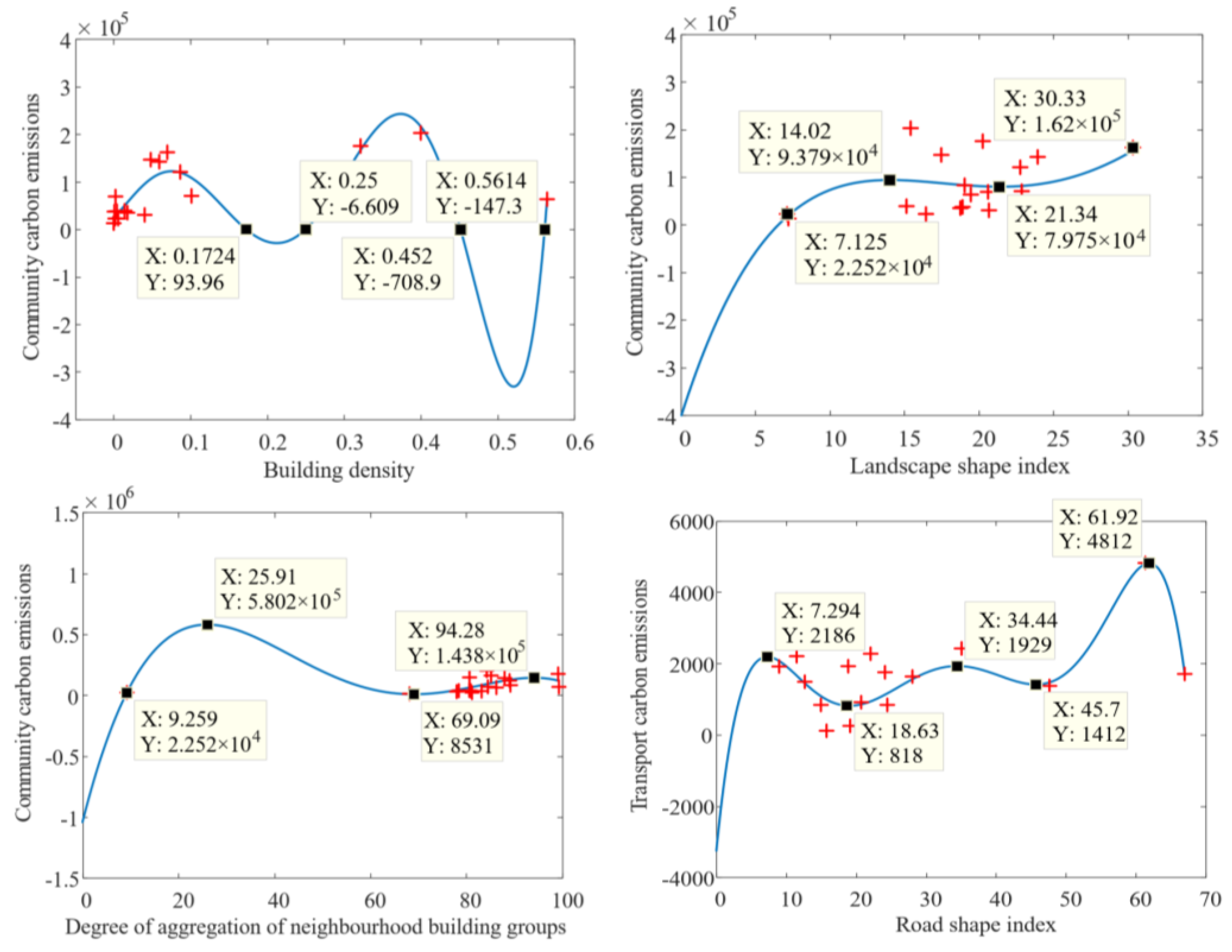
- Building density has the greatest impact on rural carbon emissions among the spatial form indicators.
- (3)
- There is a negative correlation between the form of neighborhood building groups and carbon emissions within a certain range.
4.4. Reference Values for Spatial Form Indicators
5. Discussion
6. Conclusions
Author Contributions
Funding
Institutional Review Board Statement
Informed Consent Statement
Data Availability Statement
Conflicts of Interest
| 1 | There are two views on the calculation of the carbon emission factor of wood: one believes that wood can fix carbon dioxide in the air during the growth process and considers the carbon emission factor of wood to be negative; the other believes that carbon sequestration during wood growth should not be considered in the system boundary of building carbon emission analysis. In this paper, we refer to the latter viewpoint and only consider the wood cutting and processing process to calculate the carbon emission coefficient of wood. |
References
- Liang, X.; Jin, X.; He, J.; Wang, X.; Xu, C.; Qiao, G.; Zhang, X.; Zhou, Y. Impacts of land management practice strategy on regional ecosystems: Enlightenment from ecological redline adjustment in Jiangsu, China. Land Use Policy 2022, 119, 106137. [Google Scholar]
- Lu, M.; Wei, L.; Ge, D.; Sun, D.; Zhang, Z.; Lu, Y. Spatial optimization strategy of suburban villages under the guidance of multi-regulation integration. Chin. Foreign Archit. 2021, 246, 82–88. [Google Scholar]
- Huang, Z.; Liu, Y.; Gao, J.; Peng, Z. Approach for Village Carbon Emissions Index and Planning Strategies Generation Based on Two-Stage Optimization Models. Land 2022, 11, 648. [Google Scholar]
- Ahmadi, L. The Impact of Sprawl on Transportation Energy Consumption and Transportation Carbon Footprint in Large U.S. Cities. Ph.D. Thesis, The University of Texas at Arlington, Arlington, TX, USA, 2012; pp. 58–64. [Google Scholar]
- Meen Chel, J.; Kang, M.; Kim, S. Does polycentric development produce less transportation carbon emissions? Evidence from urban form identified by night-time lights across US metropolitan areas. Atmos. Environ. Urban Clim. 2022, 44, 101223. [Google Scholar]
- Van der Borght, R.; Barbera, M.P. How urban spatial expansion influences CO2 emissions in Latin American countries. Cities 2023, 139, 104389. [Google Scholar]
- Zagow, M. Does mixed-use development in the metropolis lead to less carbon emissions? Urban Clim. 2020, 34, 100682. [Google Scholar]
- Zhu, K.; Tu, M.; Li, Y. Did Polycentric and Compact Structure Reduce Carbon Emissions? A Spatial Panel Data Analysis of 286 Chinese Cities from 2002 to 2019. Land 2022, 11, 2–15. [Google Scholar]
- Sha, W.; Chen, Y.; Wu, J.; Wang, Z. Will polycentric cities cause more CO2 emissions? A case study of 232 Chinese cities. J. Environ. Sci. 2020, 96, 33–43. [Google Scholar] [CrossRef]
- Lan, T.; Shao, G.F.; Xu, Z.B. Considerable role of urban functional form in low-carbon city development. J. Clean. Prod. 2023, 392, 136256. [Google Scholar]
- Zuo, S.; Dai, S.; Ren, Y. More fragmentized urban form more CO2 emissions? A comprehensive relationship from the combination analysis across different scales. J. Clean. Prod. 2020, 244, 118659. [Google Scholar]
- Fang, C.; Wang, S.; Li, G. Changing Urban Forms and Carbon Dioxide Emissions in China: A Case Study of 30 Provincial Capital Cities. Appl. Energy 2015, 158, 519–531. [Google Scholar]
- Echenique, M.H.; Hargreaves, A.J.; Mitchell, G.; Namdeo, A. Growing Cities Sustainably: Does Urban Form Really Matter? J. Am. Plan. Assoc. 2012, 78, 121–137. [Google Scholar]
- Wang, S.-H.; Huang, S.-L.; Huang, P.-J. Can spatial planning really mitigate carbon dioxide emissions in urban areas? A case study in Taipei, Taiwan. Landsc. Urban Plan. 2018, 169, 22–36. [Google Scholar]
- Ding, G.; Guo, J.; Pueppke, S.G.; Yi, J.; Ou, M.; Ou, W.; Tao, Y. The influence of urban form compactness on CO2 emissions and its threshold effect: Evidence from cities in China. J. Environ. Manag. 2022, 322, 116032. [Google Scholar]
- Christen, A.; Coops, N.C.; Crawford, B.R.; Kellett, R.; Liss, K.N.; Olchovski, I.; Tooke, T.R.; van der Laan, M.; Voogt, J.A. Validation of Modeled Carbon-Dioxide Emiss. Urban Neighborhood Direct Eddy-Covariance Measurements. Atmos. Environ. 2011, 45, 6057–6069. [Google Scholar] [CrossRef]
- Falahatkar, S.; Rezaei, F. Towards Low Carbon Cities: Spatio-Temporal Dynamics of Urban Form and Carbon Dioxide Emissions. Remote Sens. Appl. Soc. Environ. 2020, 18, 100317. [Google Scholar]
- Makido, Y.; Dhakal, S.; Yamagata, Y. Relationship between Urban Form and CO2 Emissions: Evidence from Fifty Japanese Cities. Urban Climate 2012, 2, 55–67. [Google Scholar]
- Palme, M.; Inostroza, L.; Villacreses, G.; Lobato-Cordero, A.; Carrasco, C. From Urban Climate to Energy Consumption. Enhancing building performance simulation by including the urban heat island effect. Energy Build. 2017, 145, 107–120. [Google Scholar]
- Qin, B.; Shao, R. The impact of urban form on residents’ direct carbon emissions—A community-based case study. Urban Plan. 2012, 36, 33–38. [Google Scholar]
- Yao, S. A study on the spatial scale of community based on low carbon perspective. J. Chang. Univ. 2012, 9, 145–146. [Google Scholar]
- Chen, F.; Zhu, D.J. A theoretical approach to low carbon city research and an empirical analysis of Shanghai. Urban Dev. Res. 2009, 16, 71–79. [Google Scholar]
- Jiang, H.Y.; Xiao, R.B.; Wu, J. Influence patterns of urban household carbon emissions and implications for the planning and design of low-carbon residential communities—Guangzhou as an example. Mod. Urban Res. 2013, 2, 101–106. [Google Scholar]
- Jin, C.; Fan, L.L.; Lu, Y.Q. Research on the layout of agrotourism based on accessibility techniques—Jiangsu Province as an example. J. Nat. Resour. 2010, 25, 1506–1518. [Google Scholar]
- Man, Z.; Zhao, R.Q.; Yuan, Y.C.; Feng, D.X.; Yang, Q.L.; Wang, S.; Yang, W.J. Influence of land mix around urban residential areas on carbon emissions of residents’ commuting traffic: An example of a typical residential area in Jiangning District, Nanjing. Hum. Geogr. 2018, 33, 70–75. [Google Scholar]
- Zhu, Z.Y.; Miao, J.J.; Cui, W. Analysis of carbon emission efficiency of intensive use of urban construction land. Geogr. Res. Dev. 2016, 35, 98–103. [Google Scholar]
- Zhang, M.; Chen, Y.R.; Zhou, H. A study on the relationship between the level of intensive land use and land use carbon emission based on panel data—Example of data from 1996 to 2010 in central cities of Hubei Province. Yangtze River Basin Resour. Environ. 2015, 24, 1464–1470. [Google Scholar]
- Qin, B.; Han, S.S. Planning parameters and household carbon emission: Evidence from high- and low-carbon neighborhoods in Beijing. Habitat Int. 2013, 37, 52–60. [Google Scholar]
- Stefano, P.; Riccardo, A.; Riccardo, M. Planning low carbon urban-rural ecosystems: An integrated transport land-use model. J. Clean. Prod. 2019, 235, 96–111. [Google Scholar]
- Zhu, X.; Zhang, T.; Gao, W.; Mei, D. Analysis on spatial pattern and driving factors of carbon emission in urban–rural fringe mixed-use communities: Cases study in east Asia. Sustainability 2020, 12, 3101. [Google Scholar]
- Wen, B.; Yang, Q.; Peng, F.; Liang, L.; Wu, S.; Xu, F. Evolutionary mechanism of vernacular architecture in the context of urbanization: Evidence from southern Hebei, China. Habitat Int. 2023, 137, 102814. [Google Scholar]
- Wen, B.; Peng, F.; Yang, Q.; Lu, T.; Bai, B.; Wu, S.; Xu, F. Monitoring the green evolution of vernacular buildings based on deep learning and multi-temporal remote sensing images. Build. Simul. 2022, 16, 151–168. [Google Scholar]
- Fan, L.Y. Research on Low Carbon Rural Space Design Strategies and Evaluation Methods Based on the Yangtze River Delta Region. Ph.D. Thesis, Zhejiang University, Zhejiang, China, 2017. [Google Scholar]
- Wu, Y.Y. Research on Low Carbon Adaptive Camping Method and Practice of Rural Community Spatial Form. Ph.D. Thesis, Zhejiang University, Zhejiang, China, 2016. [Google Scholar]
- Wang, J. Research and Practice of Rural Residential Space form in Northern Zhejiang under Low Carbon Orientation. Master’s Thesis, Zhejiang University, Hangzhou, China, 2015. [Google Scholar]
- Bin, S. Research on Low-Carbon Camping System of Urban-Rural Integrated Village Communities. Ph.D. Thesis, Zhejiang University of Technology, Zhejiang, China, 2020; pp. 46–55. [Google Scholar]
- Wu, L.Y. Generalized Architecture; Tsinghua University Press: Beijing, China, 1989. [Google Scholar]
- Zhang, X.L. The operation mechanism of Beijing urban design guidelines. Planner 2013, 29, 27–32. [Google Scholar]
- Yao, Y.H.; Lu, J.; Liu, M.R.; Lv, M.; Ji, Y. The practice of urban design in key areas of Guangzhou City under the background of fine management. Planner 2010, 26, 35–40. [Google Scholar]
- Wang, G.X.; Wu, J. The impact of urban scale and spatial structure on carbon emissions. Urban Dev. Res. 2012, 19, 89–95. [Google Scholar]
- Li, Y.H.; Fu, X.; Ma, Q.W. A preliminary investigation of low carbon rural landscape optimization strategy based on green infrastructure evaluation. West. J. Habitat Environ. 2015, 30, 11–14. [Google Scholar]
- IPCC Updates Methodology for Greenhouse Gas Inventories. Available online: https://bit.ly/2PYwytS (accessed on 23 March 2022).
- Peng, W.F.; Zhou, J.M.; Xu, X.L.; Luo, H.L.; Zhao, J.F.; Yang, C.J. Carbon emissions and carbon footprint effects and spatial and temporal patterns in Sichuan Province based on land use change. J. Ecol. 2016, 36, 7244–7259. [Google Scholar]
- GBT 51366-2019; Carbon Emission Calculation Standard for Buildings. China Construction Industry Press: Beijing, China, 2019; pp. 15–86.
- Yang, Q.M. Quantitative Evaluation of the Whole Life Cycle Environmental Impact of Building Products. Ph.D. Thesis, Tianjin University, Tianjin, China, 2009; pp. 42–46. [Google Scholar]
- Liu, Z.R.; Xu, H.P. A study on carbon emission of wood-frame buildings in the materialization stage based on type comparison. In Proceedings of the 2020 International Conference on Green Building and Building Energy Efficiency, Suzhou, China, 26–27 August 2020. [Google Scholar]
- Zhang, X.C. Research on the Calculation of Building Carbon Emission Analysis and Low Carbon Building Structure Evaluation Method. Ph.D. Thesis, Harbin Institute of Technology, Heilongjiang, China, 2018; pp. 56–60. [Google Scholar]
- Bribian, I.Z.; Capilla, A.V.; Uson, A.A. Life cycle assessment of building materials: Comparative analysis of energy and environmental impacts and evaluation of the eco-efficiency improvement potential. Build. Environ. 2011, 46, 1133–1140. [Google Scholar]
- Zhao, C.L.; Yang, B.Z. The design of pedestrian space and the choice of pedestrian transportation mode: An analysis of Jan Gehl’s theory of urban public space design. China Gard. 2012, 28, 39–42. [Google Scholar]
- Wen, B.; Yang, Q.; Xu, F.; Zhou, J.; Zhang, R. Phenomenon of courtyards being roofed and its significance for building energy efficiency. Energy Build. 2023, 295, 113282. [Google Scholar]
- Yin, C.; Xiao, J.; Zhang, T. Effectiveness of Chinese Regulatory Planning in Mitigating and Adapting to Climate Change: Comparative Analysis Based on Q Methodology. Sustainability 2021, 13, 9701. [Google Scholar]
- Yang, L.Y.; Zhang, H.H.; Luo, W.L. The Relationship between Spatial Characteristics of Urban-Rural Settlements and Carbon Emissions in Guangdong Province. Environ. Res. Public Health 2023, 20, 2659. [Google Scholar]
- Zheng, D.; Wu, H.; Lin, C.; Weng, T. Research on the integration of urban carbon reduction unit construction and planning technology based on carbon accounting. Urban Plan. J. 2021, 264, 43–50. [Google Scholar]


| Scale | Morphology | Tier 1 Indicators | Secondary Indicators | Data Collection Method |
|---|---|---|---|---|
| The overall rural community scale | Volume form | Size indicators | X1 Total land area (ha) | Land use data |
| X2 Construction land area (ha) | Land use data | |||
| Compactness of land use | X3 Building density | Calculation | ||
| Layout form | Shape complexity | X4 Perimeter area fractional dimension index (PAFRAC) | Fragstats | |
| Layout pattern | X5 Overall landscape shape index (OLSI) | Fragstats | ||
| Neighborhood building groups scale | Combination form | Settlement Aggregation | X6 Aggregation (AI) | Fragstats |
| Settlement Connectivity | X7 Connectivity index (CONNECT) | Fragstats | ||
| Connection Form | Road shape index | X8 Road network shape index (RLSI) | Fragstats | |
| Connectivity index | X9 Road patch proximity index (CONTIG) | Fragstats | ||
| Public space Accessibility | X10 Average distance to public space | Field research |
| Energy Category | Standard Coal Conversion Factor (kg Standard Coal/kg) | Carbon Emission Factor (kg/kg Standard Coal) | Energy Category | Standard Coal Conversion Factor (kg Standard Coal/kg) | Carbon Emission Factor (kg/kg Standard Coal) |
|---|---|---|---|---|---|
| Gasoline | 1.4714 | 0.5538 | Natural Gas | 1.3300 | 0.4483 |
| Liquefied Petroleum Gas | 1.7143 | 0.0030 | Power | 0.1229 kg standard coal/kWh | 0.4987 kg/KWh |
| Honeycomb Coal | 0.6302 kgC/kg | Firewood | 2.7 g/kg | ||
| The Kaiser–Meyer–Olkin Metric of Sampling Adequacy | 0.465 | |
| Bartlett’s sphericity test | Approximate cardinality | 76.009 |
| df | 28 | |
| Sig. | 0.000 | |
| Ingredients | Initial Eigenvalue | Extraction of Squares and Loading | ||||
|---|---|---|---|---|---|---|
| Total | % of Variance | Cumulative % | Total | % of Variance | Cumulative % | |
| 1 | 2.462 | 30.778 | 30.778 | 2.462 | 30.778 | 30.778 |
| 2 | 2.361 | 29.507 | 60.285 | 2.361 | 29.507 | 60.285 |
| 3 | 1.623 | 20.285 | 80.57 | 1.623 | 20.285 | 80.57 |
| 4 | 0.81 | 10.121 | 90.692 | |||
| 5 | 0.405 | 5.068 | 95.76 | |||
| 6 | 0.165 | 2.068 | 97.827 | |||
| 7 | 0.11 | 1.379 | 99.206 | |||
| 8 | 0.063 | 0.794 | 100 | |||
| Component | |||
|---|---|---|---|
| 1 | 2 | 3 | |
| Z-score (LNX)1 | 0.137 | 0.259 | 0.359 |
| Z-score (LNX)3 | 0.079 | −0.204 | −0.383 |
| Z-score (LNX)4 | −0.27 | 0.27 | −0.129 |
| Z-score (LNX)5 | 0.376 | 0.08 | −0.016 |
| Z-score (LNX)6 | 0.294 | 0.087 | −0.32 |
| Z-score (LNX)7 | 0.179 | −0.35 | 0.155 |
| Z-score (LNX)8 | 0.206 | 0.318 | −0.07 |
| Z-score (LN)10 | 0.075 | −0.069 | 0.438 |
| Liaoyuan Village | Jinhua Village | Wangxing Village | Traffic Village | |
|---|---|---|---|---|
| Northern Hunan Region | 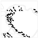 |  | 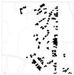 |  |
| Zhushan Village | Penglang Village | Songshan Village | Hegun Village | |
| Xiangxi Region | 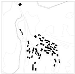 | 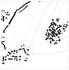 | 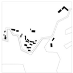 | 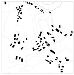 |
| Shimen Village | Gwangyang Village | Yongfu Village | Shidu Village | |
| Central Hunan Region |  | 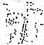 | 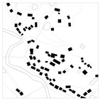 | 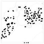 |
| Hantian Village | Shazhou Village | Xiushui Village | Wazao Village | |
| Southern Hunan Region | 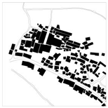 | 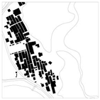 | 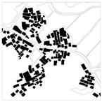 |  |
| Total Land Area | Construction Land Area | Building Density | PAFRAC | OLSI | AI | CONNECT | RLSI | CONTIG | Average Distance | |
|---|---|---|---|---|---|---|---|---|---|---|
| Liaoyuan Village | 811.40 | 45.81 | 0.06 | 1.65 | 20.61 | 99.32 | 2.42 | 67.00 | 0.45 | 308.10 |
| Jiao Long Village | 748.05 | 188.36 | 0.20 | 1.30 | 19.04 | 89.21 | 65.22 | 20.71 | 0.60 | 398.69 |
| Shaoshan Village | 16.83 | 2.70 | 0.16 | 1.26 | 15.42 | 84.29 | 100.00 | 11.49 | 0.66 | 314.72 |
| Tianhan Village | 1185.95 | 150.50 | 0.17 | 1.12 | 17.47 | 80.68 | 98.59 | 35.08 | 0.20 | 417.41 |
| Qingting Village | 350.00 | 36.36 | 0.10 | 1.25 | 22.77 | 89.04 | 93.49 | 24.45 | 0.50 | 428.51 |
| Lutang Village | 860.14 | 193.46 | 0.22 | 1.63 | 20.26 | 99.16 | 1.23 | 61.37 | 0.40 | 345.52 |
| Ma Ying Tong | 400.00 | 19.00 | 0.05 | 1.72 | 18.90 | 80.95 | 0.00 | 28.05 | 0.53 | 271.19 |
| Zhushan Village | 476.76 | 18.62 | 0.04 | 1.12 | 16.44 | 81.21 | 100.00 | 18.85 | 0.46 | 671.79 |
| Penglang Village | 1376.88 | 22.53 | 0.02 | 1.12 | 20.67 | 78.00 | 99.47 | 15.76 | 0.57 | 365.49 |
| Little Fishing Creek | 2100.00 | 9.00 | 0.00 | 1.72 | 15.14 | 80.64 | 0.00 | 24.13 | 0.53 | 239.13 |
| Shuangqiao Village | 1610.43 | 46.39 | 0.02 | 1.27 | 25.85 | 78.45 | 0.78 | 47.65 | 0.48 | 390.12 |
| Xiuzhou Village | 551.68 | 17.00 | 0.03 | 1.57 | 7.13 | 9.26 | 20.39 | 8.98 | 0.22 | 467.52 |
| Shituo Village | 244.57 | 23.42 | 0.10 | 1.09 | 18.75 | 83.20 | 99.63 | 19.13 | 0.66 | 380.85 |
| Wushan Village | 1036.55 | 39.80 | 0.04 | 1.09 | 22.87 | 84.50 | 100.00 | 22.06 | 0.60 | 341.71 |
| Wazao Village | 324.95 | 54.82 | 0.17 | 1.09 | 19.45 | 86.27 | 98.05 | 21.25 | 0.65 | 248.27 |
| Ishizen Village | 1384.53 | 69.17 | 0.05 | 1.09 | 30.33 | 85.18 | 96.94 | 28.11 | 0.54 | 309.60 |
| Shazhou Village | 92.62 | 10.77 | 0.12 | 1.60 | 7.21 | 68.17 | 0.00 | 12.65 | 0.60 | 187.78 |
| Hongxing Village | 369.29 | 66.77 | 0.18 | 1.08 | 23.94 | 87.99 | 99.77 | 14.96 | 0.64 | 188.51 |
| Building Type | Construction Phase | Operation Phase/Year | Total | Carbon Emission Intensity |
|---|---|---|---|---|
| Brick and mortar building | 157,477.14 kg | 4492.17 kg | 161,969.31 kg | 489.69 kg/m2 |
| Wooden architecture | 31,431.85 kg | 2652.37 kg | 34,084.22 kg | 324.61 kg/m2 |
| Liaoyuan Village | Jiao Long Community | Shaoshan Village | Tianhan Village | Green Pavilion Village | Lutang Village | |
|---|---|---|---|---|---|---|
| Distance traveled/km | 2880.00 | 2160.00 | 8400.20 | 5564.20 | 389.33 | 1945.20 |
| Carbon emissions | 1241.74 | 931.31 | 2204.42 | 2423.15 | 839.32 | 838.69 |
| Ma Ying Tong Village | Zhushan Village | Penglang Village | Little Fishery Creek Village | Shuangqiao Village | Xiuzhou Village | |
| Distance traveled/km | 432.00 | 8929.17 | 521.43 | 520.80 | 1167.36 | 393.60 |
| Carbon emissions | 186.26 | 1924.95 | 112.41 | 224.55 | 503.32 | 169.70 |
| Wushan Village | Wazao Village | Ishizen Village | Shazhou Village | Hongxing Village | Shituo Village | |
| Distance traveled/km | 677.76 | 935.10 | 3615.24 | 743.04 | 4505.14 | 1160.22 |
| Carbon emissions | 292.22 | 60.48 | 338.73 | 320.37 | 839.03 | 250.12 |
| Calculation of Carbon Emissions | Construction Phase | Operation Phase | Total Carbon Emissions/t | |||||
|---|---|---|---|---|---|---|---|---|
| Number of Households | Building Area/m2 | Carbon Emission Intensity/kg | Energy Carbon Emission/kg | Transportation Carbon Emission/kg | ||||
| Northern Hunan Region | 1 | Liaoyuan Village | 775 | 168.06 | 489.69 | 2787.06 | 1201.67 | 66,871.68 |
| 2 | Jiao Long Village | 765 | 212.31 | 489.69 | 1650.66 | 711.7 | 80,306.24 | |
| 3 | Shaoshan Village | 1355 | 283.56 | 489.69 | 4467.58 | 2204.42 | 197,191.10 | |
| 4 | Tianhan Village | 736 | 375 | 489.69 | 7145.50 | 2423.15 | 141,097.95 | |
| 5 | Qingting Village | 840 | 280 | 489.69 | 2746.43 | 839.32 | 116,820.63 | |
| 6 | Lutang Village | 1040 | 308.09 | 489.69 | 7027.94 | 4819.72 | 164,355.68 | |
| Western Hunan Region | 7 | Ma Ying Tong | 601 | 164.46 | 324.61 | 2836.51 | 1635.13 | 34,524.36 |
| 8 | Zhushan Village | 302 | 180 | 324.61 | 7844.09 | 1924.95 | 20,596.05 | |
| 9 | Penglang Village | 386 | 200.21 | 324.61 | 6368.33 | 112.41 | 27,587.77 | |
| 10 | Little Fishing Creek | 700 | 144.36 | 324.61 | 2941.28 | 1754.41 | 35,749.09 | |
| 11 | Shuangqiao Village | 672 | 150.66 | 324.61 | 2537.42 | 1369.39 | 35,305.00 | |
| 12 | Xiuzhou Village | 347 | 170 | 324.61 | 3227.43 | 1916.64 | 20,751.52 | |
| Central Hunan | 13 | Shito Village | 377 | 179.19 | 489.69 | 2239.94 | 250.12 | 33,408.60 |
| Southern Hunan Region | 14 | Wushan Village | 729 | 179.19 | 489.69 | 3818.60 | 2273.09 | 67,951.97 |
| 15 | Wazao Village | 394 | 304.29 | 489.69 | 6345.81 | 60.48 | 60,490.42 | |
| 16 | Ishizen Village | 1098 | 283.33 | 489.69 | 4705.72 | 338.73 | 157,879.57 | |
| 17 | Shazhou Village | 142 | 172.19 | 489.69 | 2429.67 | 1487.81 | 12,467.17 | |
| 18 | Hongxing Village | 585 | 460 | 489.69 | 9739.01 | 839.03 | 135,940.59 | |
| Equation (1) | Compound Correlation Coefficient | 0.781 |
| R-Square | 0.61 | |
| Adjustment of R-Square | 0.526 | |
| Estimated Standard Error | 0.318 |
| Number of Households | 8 | 12 | 16 | 20 | 24 |
|---|---|---|---|---|---|
| Layout |  |  |  |  |  |
| Carbon emissions per unit of floor space | 7.8682 | 7.8707 | 7.8720 | 7.8732 | 7.8732 |
| Rows | 4 × 2 | 3 × 3 | 4 × 3 | 3 × 5 | 4 × 4 | 4 × 5 | 5 × 5 | 5 × 6 |
|---|---|---|---|---|---|---|---|---|
| Building density | 8.28% | 9.31% | 12.41% | 15.52% | 16.55% | 20.69% | 25.86% | 31.04% |
| T-Shaped | Lineage | Wrong Column | Oblique Column | Freestyle |
|---|---|---|---|---|
 |  |  |  | 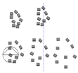 |
Disclaimer/Publisher’s Note: The statements, opinions and data contained in all publications are solely those of the individual author(s) and contributor(s) and not of MDPI and/or the editor(s). MDPI and/or the editor(s) disclaim responsibility for any injury to people or property resulting from any ideas, methods, instructions or products referred to in the content. |
© 2023 by the authors. Licensee MDPI, Basel, Switzerland. This article is an open access article distributed under the terms and conditions of the Creative Commons Attribution (CC BY) license (https://creativecommons.org/licenses/by/4.0/).
Share and Cite
Song, L.; Xu, F.; Sheng, M.; Wen, B. The Relationship between Rural Spatial Form and Carbon Emission—A Case Study of Suburban Integrated Villages in Hunan Province, China. Land 2023, 12, 1585. https://doi.org/10.3390/land12081585
Song L, Xu F, Sheng M, Wen B. The Relationship between Rural Spatial Form and Carbon Emission—A Case Study of Suburban Integrated Villages in Hunan Province, China. Land. 2023; 12(8):1585. https://doi.org/10.3390/land12081585
Chicago/Turabian StyleSong, Limei, Feng Xu, Ming Sheng, and Baohua Wen. 2023. "The Relationship between Rural Spatial Form and Carbon Emission—A Case Study of Suburban Integrated Villages in Hunan Province, China" Land 12, no. 8: 1585. https://doi.org/10.3390/land12081585