
Water Quality Determination Using Soil and Vegetation Communities in the Wetlands of the Andes of Ecuador
 , , , , , and
Abstract
:1. Introduction
2. Materials and Methods
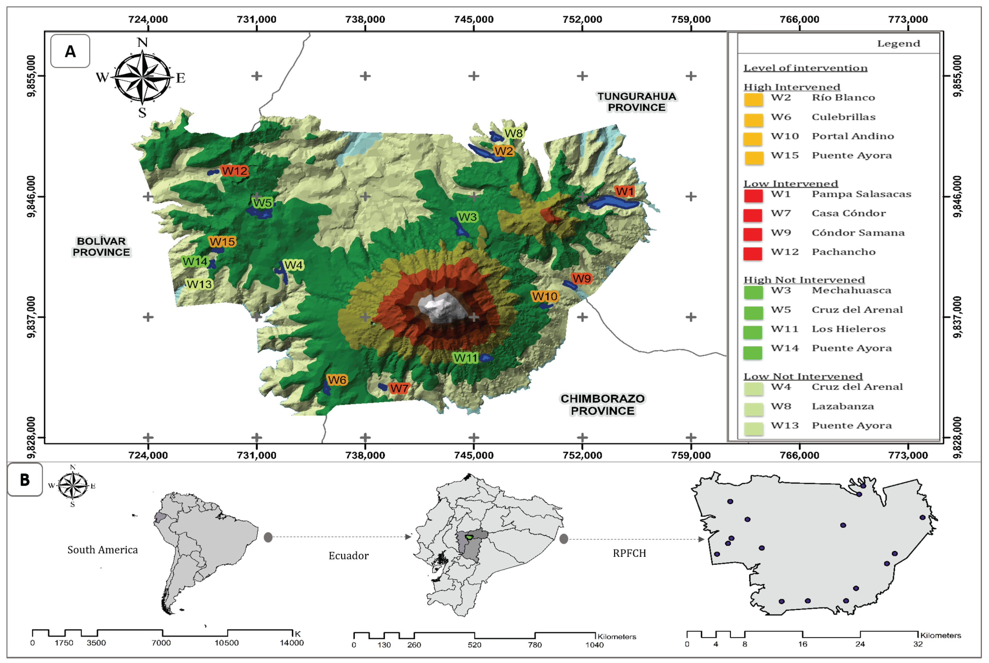
2.1. Study Area
2.2. Floristic Sampling and Inventory
2.3. Measurement of Selected Physicochemical Variables: Collection and Analysis of Water Samples
2.4. Soil Sampling and Analysis
2.5. Data Analysis
3. Results
3.1. Floristic Inventory
3.2. Physicochemical Analysis of Water
3.3. Soil Analysis
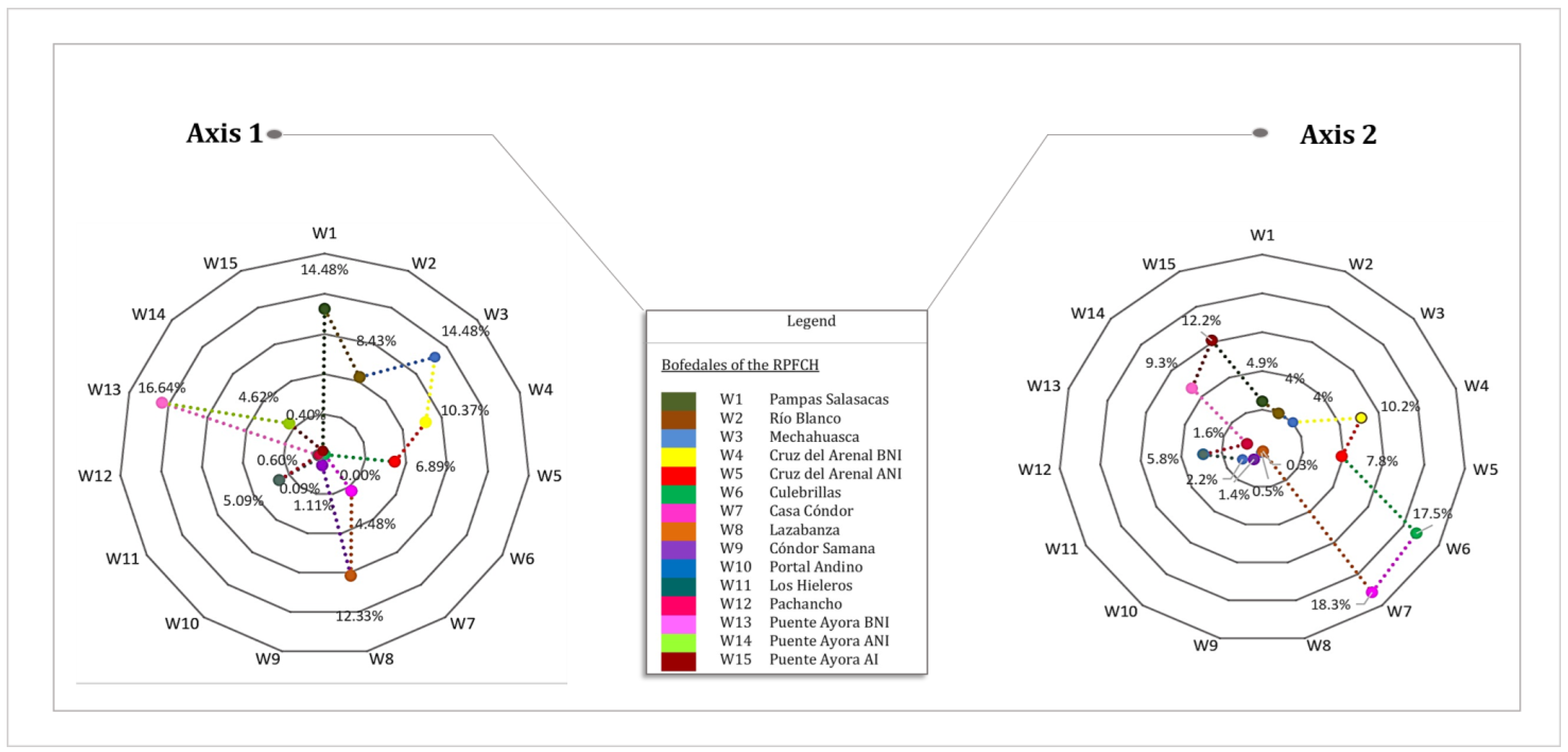
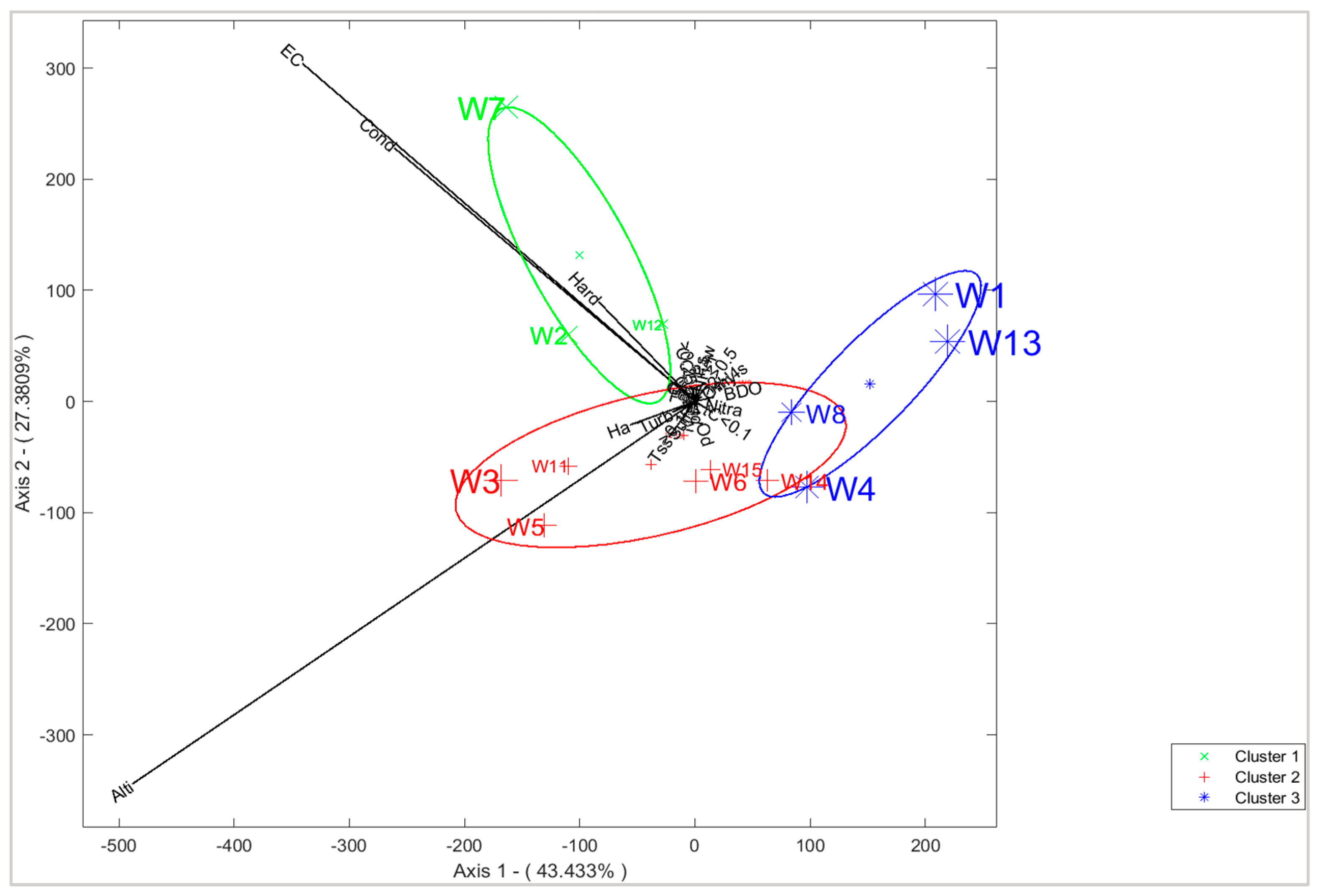
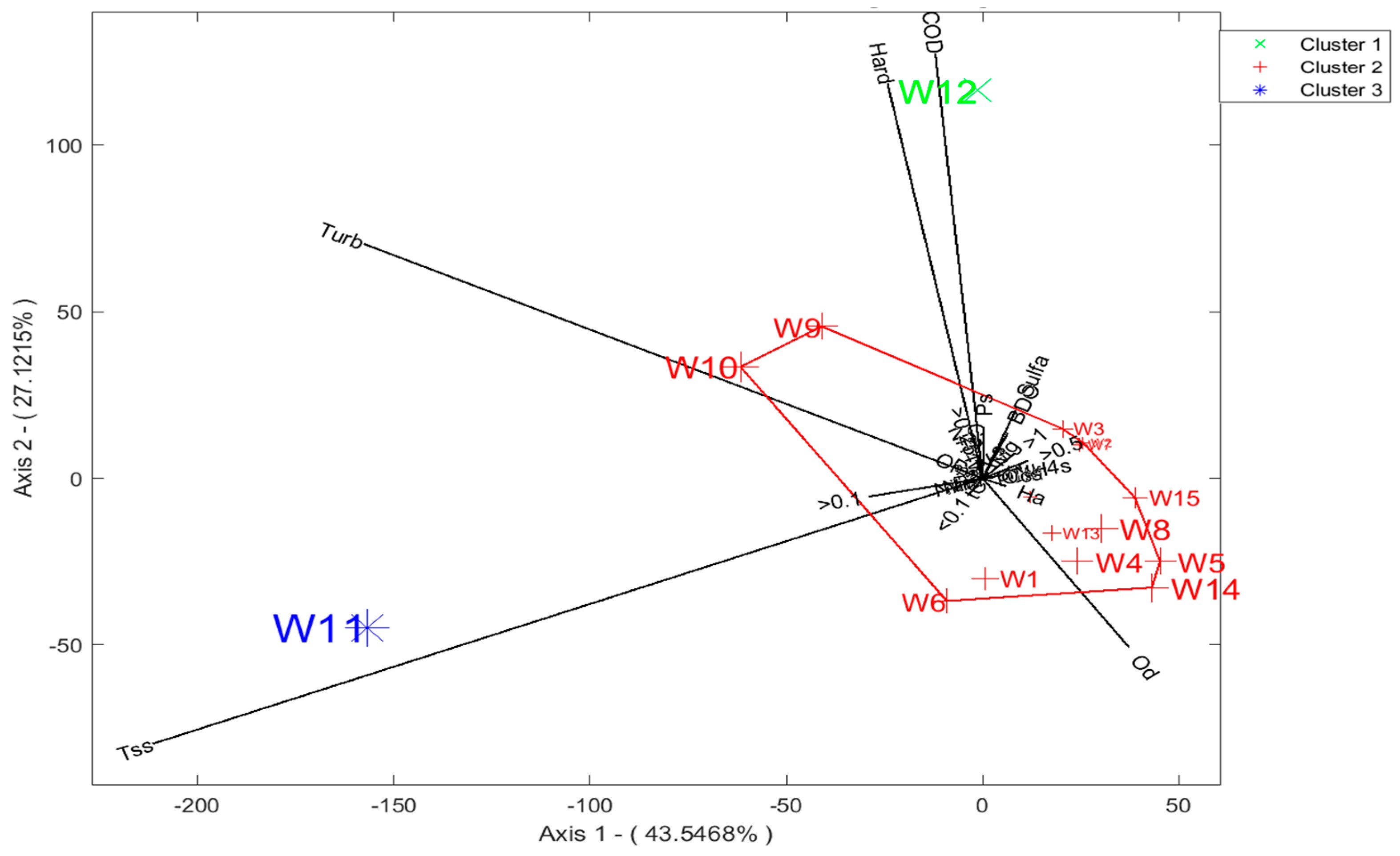
3.4. Characterization of Sites with Soil and Water Variables
4. Discussion
5. Conclusions
Author Contributions
Funding
Data Availability Statement
Acknowledgments
Conflicts of Interest
Appendix A

| Bofedal | Province | Latitude | Longitude | Altitude (m.a.s.l.) | Total Area (ha) | Ecological Classification |
|---|---|---|---|---|---|---|
| Los Hieleros ANI | Chimborazo | 745,741 | 9,833,916 | 4442 | 25.67 | Subnival evergreen moorland grassland and shrubland |
| Culebrillas IA | Chimborazo | 735,446 | 9,831,848 | 4160 | 13.31 | Páramo flooded grassland |
| Casa Cóndor BI | Chimborazo | 739,244 | 9,831,672 | 4008 | 9.40 | Páramo flooded grassland |
| Lazabanza BNI | Tungurahua | 746,734 | 9,850,338 | 4039 | 26.46 | Subnival moorland humid grassland |
| Cóndor Samana BI | Tungurahua | 751,109 | 9,839,489 | 3825 | 21.36 | Páramo upper montane moist upper montane grassland |
| Pampas Salasacas BI | Tungurahua | 754,972 | 9,845,283 | 3854 | 154.40 | Páramo upper montane moist upper montane grassland |
| Río Blanco AI | Tungurahua | 746,179 | 9,849,003 | 4016 | 65.44 | Evergreen shrubland and moorland grassland |
| Mechahuasca ANI | Tungurahua | 743,954 | 9,844,037 | 4240 | 35.48 | Páramo Grassland |
| Portal Andino AI | Chimborazo | 750,019 | 9,837,891 | 4120 | 7.62 | Subnival evergreen grassland and shrubland of the moorland |
| Cruz del Arenal ANI | Bolívar | 731,162 | 9,844,778 | 4240 | 57.75 | Subnival evergreen grassland and shrubland of the moorland |
| Puente Ayora ANI | Bolívar | 728,478 | 9,841,941 | 4105 | 12.19 | Subnival evergreen grassland and shrubland of the moorland |
| Puente Ayora BNI | Bolívar | 726,486 | 9,839,401 | 3842 | 0.29 | Evergreen shrubland and moorland grassland |
| Puente Ayora AI | Bolívar | 728,013 | 9,841,127 | 4120 | 12.84 | Subnival evergreen grassland and shrubland of the moorland |
| Pachancho BI | Bolívar | 728,315 | 9,847,854 | 4040 | 8.78 | Subnival evergreen grassland and shrubland of the moorland |
| Cruz del Arenal BNI | Bolívar | 732,671 | 9,840,421 | 4120 | 18.78 | Páramo upper montane moist upper montane grassland |
References
- Beller, E.E.; McClenachan, L.; Zavaleta, E.S.; Larsen, L.G. Past forward: Recommendations from historical ecology for ecosystem management. Glob. Ecol. Conserv. 2020, 21, e00836. [Google Scholar] [CrossRef]
- Allan, J.D. Landscapes and Riverscapes: The Influence of Land Use on Stream Ecosystems. Annu. Rev. Ecol. Evol. Syst. 2004, 35, 257–284. [Google Scholar] [CrossRef] [Green Version]
- Sánchez, O. Perspectivas Sobre Conservación de Ecosistemas Acuáticos en México; Instituto Nacional de Ecología: Mexico City, Mexico, 2007. [Google Scholar]
- Withey, P.; van Kooten, G.C. The effect of climate change on optimal wetlands and waterfowl management in Western Canada. Ecol. Econ. 2011, 70, 798–805. [Google Scholar] [CrossRef]
- Xia, S.; Liu, Y.; Chen, B.; Jia, Y.; Zhang, H.; Liu, G.; Yu, X. Effect of water level fluctuations on wintering goose abundance in Poyang Lake wetlands of China. Chin. Geogr. Sci. 2017, 27, 248–258. [Google Scholar] [CrossRef] [Green Version]
- Finlayson, C.M.; Davidson, N.C.; Spiers, A.G.; Stevenson, N.J. Global wetland inventory—Current status and future priorities. Mar. Freshw. Res. 1999, 50, 717–727. [Google Scholar] [CrossRef]
- Costanza, R.; de Groot, R.; Sutton, P.; van der Ploeg, S.; Anderson, S.J.; Kubiszewski, I.; Farber, S.; Turner, R.K. Changes in the global value of ecosystem services. Glob. Environ. Chang. 2014, 26, 152–158. [Google Scholar] [CrossRef]
- Global Wetland Outlook. (s.f.). Global Wetland Outlook. Recuperado 9 de junio de 2023. Available online: https://www.global-wetland-outlook.ramsar.org (accessed on 8 February 2022).
- Blanco, D. Los Turbales de la Patagonia. Bases Para su Inventario y la Conservación de su Biodiversidad; En Hemeroteca CEDOC CIREN; Wetlands International—América del Sur: Buenos Aires, Argentina, 2004; Available online: https://bibliotecadigital.ciren.cl/handle/20.500.13082/26803 (accessed on 8 February 2022).
- Moreno-Mateos, D.; Power, M.E.; Comín, F.A.; Yockteng, R. Structural and Functional Loss in Restored Wetland Ecosystems. PLoS Biol. 2012, 10, e1001247. [Google Scholar] [CrossRef] [PubMed] [Green Version]
- Costanza, R.; d’Arge, R.; de Groot, R.; Farber, S.; Grasso, M.; Hannon, B.; Limburg, K.; Naeem, S.; O’Neill, R.V.; Paruelo, J.; et al. The value of the world’s ecosystem services and natural capital. Nature 1997, 387, 6630. [Google Scholar] [CrossRef]
- Junk, W.J.; An, S.; Finlayson, C.M.; Gopal, B.; Květ, J.; Mitchell, S.A.; Mitsch, W.J.; Robarts, R.D. Current state of knowledge regarding the world’s wetlands and their future under global climate change: A synthesis. Aquat. Sci. 2013, 75, 151–167. [Google Scholar] [CrossRef] [Green Version]
- Barbier, E.; Acreman, M.; Knowler, D. Valoración Económica de los Humedales; Oficina de la Convención de Ramsar: Gland, Switzerland, 1997; Available online: https://portals.iucn.org/library/sites/library/files/documents/Ramsar-021-Es.pdf (accessed on 8 February 2022).
- Bragazza, L.; Rydin, H.; Gerdol, R. Multiple gradients in mire vegetation: A comparison of a Swedish and an Italian bog. Plant Ecol. 2005, 177, 223–236. [Google Scholar] [CrossRef]
- Sottocornola, M.; Laine, A.; Kiely, G.; Byrne, K.A.; Tuittila, E.-S. Vegetation and environmental variation in an Atlantic blanket bog in South-western Ireland. Plant Ecol. 2009, 203, 69–81. [Google Scholar] [CrossRef]
- Glina, B.; Piernik, A.; Hulisz, P.; Mendyk, Ł.; Tomaszewska, K.; Podlaska, M.; Bogacz, A.; Spychalski, W. Water or soil—What is the dominant driver controlling the vegetation pattern of degraded shallow mountain peatlands? Land Degrad. Dev. 2019, 30, 1437–1448. [Google Scholar] [CrossRef]
- Gallant, A.L. The Challenges of Remote Monitoring of Wetlands. Remote Sens. 2015, 7, 10938–10950. [Google Scholar] [CrossRef] [Green Version]
- Buytaert, W.; Célleri, R.; de Bièvre, B.; Cisneros, F. Hidrología del Páramo Andino: Propiedades. Importancia y Vulnerabilidad. 2023. Available online: https://www.researchgate.net/publication/228459137_HIDROLOGIA_DEL_PARAMO_ANDINO_PROPIEDADES_IMPORTANCIA_Y_VULNERABILIDAD (accessed on 8 February 2022).
- Flachier, A.; Chinchero, M.; Lima, P.; Villarroel, M. Caracterización Ecológica de las Turberas y Bofedales del Sistema de Humedales Amaluza. In Nudo de Sabanilla, Provincia de Loja, Ecuador; Ministerio del Ambiente: Lima, Peru, 2009; Available online: https://docplayer.es/57884650-Caracterizacion-ecologica-de-las-turberas-y-bofedales-del-sistema-de-humedales-amaluza-nudo-de-sabanilla-provincia-de-loja-ecuador.html (accessed on 15 July 2022).
- Jara, C.; Delegido, J.; Ayala, J.; Lozano, P.; Armas, A.; Flores, V. Estudio de bofedales en los Andes ecuatorianos a través de la comparación de imágenes Landsat-8 y Sentinel-2. Rev. Teledetec. 2019, 53, 45. [Google Scholar] [CrossRef] [Green Version]
- Conferencia de las Partes. Estrategia Regional de Conservación y Uso Sostenible de los Humedales Altoandinos. In Proceedings of the 9a Reunión de la Conferencia de las Partes Contratantes en la Convención sobre los Humedales, Kampala, Uganda, 8–15 November 2005; Available online: https://www.ramsar.org/sites/default/files/documents/pdf/cop9/cop9_doc26_s.pdf (accessed on 15 July 2022).
- Guo, Z.; Cui, G.; Zhang, M.; Li, X. Analysis of the contribution to conservation and effectiveness of the wetland reserve network in China based on wildlife diversity. Glob. Ecol. Conserv. 2019, 20, e00684. [Google Scholar] [CrossRef]
- Geldmann, J.; Coad, L.; Barnes, M.; Craigie, I.D.; Hockings, M.; Knights, K.; Leverington, F.; Cuadros, I.C.; Zamora, C.; Woodley, S.; et al. Changes in protected area management effectiveness over time: A global analysis. Biol. Conserv. 2015, 191, 692–699. [Google Scholar] [CrossRef] [Green Version]
- UNEP; WCMC; UICN. The Lag Effect in the World Database on Protected Areas. Protected Planet. 2018. Available online: https://www.protectedplanet.net/en/news-and-stories/the-lag-effect-in-the-world-database-on-protected-areas (accessed on 25 July 2022).
- Ministerio del Ambiente del Ecuador. Áreas Protegidas—Ministerio del Ambiente. Agua y Transición Ecológica. Áreas Protegidas. 2014. Available online: https://www.ambiente.gob.ec/areas-protegidas-3/ (accessed on 13 August 2022).
- McLaren, B.E.; MacNearney, D.; Siavichay, C.A. Livestock and the functional habitat of vicuñas in Ecuador: A new puzzle. Ecosphere 2018, 9, e02066. [Google Scholar] [CrossRef] [Green Version]
- Hill, B.H.; Jicha, T.M.; Lehto, L.L.P.; Elonen, C.M.; Sebestyen, S.D.; Kolka, R.K. Comparisons of soil nitrogen mass balances for an ombrotrophic bog and a minerotrophic fen in northern Minnesota. Sci. Total Environ. 2016, 550, 880–892. [Google Scholar] [CrossRef]
- Nicia, P.; Bejger, R.; Zadrożny, P.; Sterzyńska, M. The impact of restoration processes on the selected soil properties and organic matter transformation of mountain fens under Caltho-Alnetum community in the Babiogórski National Park in Outer Flysch Carpathians. Poland. J. Soils Sediments 2018, 18, 2770–2776. [Google Scholar] [CrossRef] [Green Version]
- Griffiths, N.A.; Sebestyen, S.D.; Oleheiser, K.C. Variation in peatland porewater chemistry over time and space along a bog to fen gradient. Sci. Total Environ. 2019, 697, 134152. [Google Scholar] [CrossRef]
- White, D.A.; Weiss, T.E.; Trapani, J.M.; Thien, L.B. Productivity and Decomposition of the Dominant Salt Marsh Plants in Louisiana. Ecology 1978, 59, 751–759. [Google Scholar] [CrossRef]
- Simas, T.; Ferreira, J. Nutrient enrichment and the role of salt marshes in the Tagus estuary (Portugal). Estuar. Coast. Shelf Sci. 2007, 75, 393–407. [Google Scholar] [CrossRef]
- Van Donk, E.; van de Bund, W.J. Impact of submerged macrophytes including charophytes on phyto- and zooplankton communities: Allelopathy versus other mechanisms. Aquat. Bot. 2002, 72, 261–274. [Google Scholar] [CrossRef]
- Wetzel, R.; Hough, R. Productivity and Role of Aquatic Macrophytes in Lakes: An Assessment; COO-1599-54; CONF-720620-1; Michigan State University: Lansing, MI, USA, 1972. Available online: https://www.osti.gov/servlets/purl/4639975 (accessed on 17 August 2022).
- Zhang, Y.; Jeppesen, E.; Liu, X.; Qin, B.; Shi, K.; Zhou, Y.; Thomaz, S.M.; Deng, J. Global loss of aquatic vegetation in lakes. Earth-Sci. Rev. 2017, 173, 259–265. [Google Scholar] [CrossRef]
- Gong, H.; Gao, J. Soil and climatic drivers of plant SLA (specific leaf area). Glob. Ecol. Conserv. 2019, 20, e00696. [Google Scholar] [CrossRef]
- Carreño-Rocabado, G.; Peña-Claros, M.; Bongers, F.; Díaz, S.; Quétier, F.; Chuviña, J.; Poorter, L. Land-use intensification effects on functional properties in tropical plant communities. Ecol. Appl. 2016, 26, 174–189. [Google Scholar] [CrossRef] [Green Version]
- Chillo, V.; Vázquez, D.P.; Amoroso, M.M.; Bennett, E.M. Land-use intensity indirectly affects ecosystem services mainly through plant functional identity in a temperate forest. Funct. Ecol. 2018, 32, 1390–1399. [Google Scholar] [CrossRef] [Green Version]
- Peco, B.; Navarro, E.; Carmona, C.P.; Medina, N.G.; Marques, M.J. Effects of grazing abandonment on soil multifunctionality: The role of plant functional traits. Agric. Ecosyst. Environ. 2017, 249, 215–225. [Google Scholar] [CrossRef]
- Díaz, S.; Lavorel, S.; de Bello, F.; Quétier, F.; Grigulis, K.; Robson, T.M. Incorporating plant functional diversity effects in ecosystem service assessments. Proc. Natl. Acad. Sci. USA 2007, 104, 20684–20689. [Google Scholar] [CrossRef]
- Wen, Z.; Zheng, H.; Smith, J.R.; Zhao, H.; Liu, L.; Ouyang, Z. Functional diversity overrides community-weighted mean traits in linking land-use intensity to hydrological ecosystem services. Sci. Total Environ. 2019, 682, 583–590. [Google Scholar] [CrossRef]
- Klaus, V.H.; Kleinebecker, T.; Busch, V.; Fischer, M.; Hölzel, N.; Nowak, S.; Prati, D.; Schäfer, D.; Schöning, I.; Schrumpf, M.; et al. Land use intensity. rather than plant species richness. affects the leaching risk of multiple nutrients from permanent grasslands. Glob. Chang. Biol. 2018, 24, 2828–2840. [Google Scholar] [CrossRef] [Green Version]
- Fischer, C.; Leimer, S.; Roscher, C.; Ravenek, J.; de Kroon, H.; Kreutziger, Y.; Baade, J.; Beßler, H.; Eisenhauer, N.; Weigelt, A.; et al. Plant species richness and functional groups have different effects on soil water content in a decade-long grassland experiment. J. Ecol. 2019, 107, 127–141. [Google Scholar] [CrossRef] [Green Version]
- Villegas, J.C. Análisis del Conocimiento en la Relación Agua-Suelo-Vegetación Para el Departamento de Antioquia. Rev. EIA 2004, 1, 73–79. [Google Scholar]
- Matteucci, S.; Colma, A. Metodología Para el Estudio de la Vegetación; En Serbiula (Sistema Librum 2.0); Universidad Nacional Experimental Francisco de Miranda: Falcón, Venezuela, 1982. [Google Scholar]
- American Public Health Association (APHA). Standard Methods for the Examination of Water and Wastewater; American Public Health Association: Washington, DC, USA, 1999. [Google Scholar]
- Red de Laboratorios de Suelos del Ecuador (RELASE). Manual para Análisis de Suelo; 2001. Available online: https://www.agrocalidad.gob.ec/wp-content/uploads/2021/08/FICHA-INIAP-2021-1.pdf (accessed on 13 August 2022).
- R Core Team. (2020) R: A Language and Environment for Statistical Computing. R Foundation for Statistical Computing, Vienna, Austria. Available online: https://www.r-project.org/ (accessed on 13 August 2022).
- Wold, S.; Esbensen, K.; Geladi, P. Principal component analysis. Chemom. Intell. Lab. Syst. 1987, 2, 37–52. [Google Scholar] [CrossRef]
- Husson, F.; Josse, J.; Le, S.; Mazet, J. FactoMineR: Multivariate Exploratory Data Analysis and Data Mining, Version 2.8; RStudio: Boston, MA, USA, 2023; Available online: https://cran.r-project.org/web/packages/FactoMineR/index.html (accessed on 13 August 2022).
- Wickham, H. Ggplot2. Rev. Comput. Stat. 2011, 3, 180–185. [Google Scholar] [CrossRef]
- Muriithi, F.K.; Yu, D. Understanding the Impact of Intensive Horticulture Land-Use Practices on Surface Water Quality in Central Kenya. Environments 2015, 2, 521–545. [Google Scholar] [CrossRef] [Green Version]
- Jabbar, F.K.; Grote, K. Statistical assessment of nonpoint source pollution in agricultural watersheds in the Lower Grand River watershed. MO. USA. Environ. Sci. Pollut. Res. 2019, 26, 1487–1506. [Google Scholar] [CrossRef] [Green Version]
- Galindo-Villardón, P. Contribuciones a la Representación Simultánea de Datos Multidimensionales. Ph.D. Thesis, Universidad de Salamanca, Salamanca, Spain, 1985; p. 1. Available online: https://dialnet.unirioja.es/servlet/tesis?codigo=287930 (accessed on 12 August 2022).
- Eckart, C.; Young, G. The approximation of one matrix by another of lower rank. Psychometrika 1936, 1, 211–218. [Google Scholar] [CrossRef]
- Galindo-Villardón, P. Una alternativa de representación simultánea. HJ-Biplot 1986, 10, 13–23. [Google Scholar]
- León-Yánez, S.; Valencia, R.; Pitman, N.; Endara, L.; Ulloa, C.; Navarrete, H. Libro Rojo de las Plantas Endémicas del Ecuador; Pontificia Universidad Católica del Ecuador. Quito. 2011. Available online: https://bioweb.bio/floraweb/librorojo/home (accessed on 12 August 2022).
- Heinselman, M.L. Landscape Evolution. Peatland Types. and the Environment in the Lake Agassiz Peatlands Natural Area. Minnesota. Ecol. Monogr. 1970, 40, 235–261. [Google Scholar] [CrossRef]
- Verhoeven, J.T.A.; Maltby, E.; Schmitz, M.B. Nitrogen and Phosphorus Mineralization in Fens and Bogs. J. Ecol. 1990, 78, 713–726. [Google Scholar] [CrossRef] [Green Version]
- Miserere, L.; Montacchini, F.; Buffa, G. Ecology of some mire and bog plant communities in the Western Italian Alps. J. Limnol. 2003, 62, 88. [Google Scholar] [CrossRef] [Green Version]
- Smith, J.M.B.; Cleef, A.M. Composition and Origins of the World’s Tropicalpine Floras. J. Biogeogr. 1988, 15, 631–645. [Google Scholar] [CrossRef]
- Sklenář, P.; Dušková, E.; Balslev, H. Tropical and Temperate: Evolutionary History of Páramo Flora. Bot. Rev. 2011, 77, 71–108. [Google Scholar] [CrossRef]
- Madriñán, S.; Cortés, A.J.; Richardson, J.E. Páramo is the world’s fastest evolving and coolest biodiversity hotspot. Front. Genet. 2013, 4, 192. Available online: https://www.frontiersin.org/articles/10.3389/fgene.2013.00192 (accessed on 24 August 2022). [CrossRef] [Green Version]
- Fonkén, M.S.M. An introduction to the bofedales of the Peruvian High Andes. Mires Peat 2014, 15, 1–13. [Google Scholar]
- Passuni, E.O.; Fonkén, M.S.M. Relationships between aquatic invertebrates. water quality and vegetation in an Andean peatland system. Mires Peat 2015, 15, 1–4. [Google Scholar]
- Troll, C. The cordilleras of the Tropical Americas. aspects of climatic. phytogeographical and agrarian ecology. Colloq. Geogr. 1968, 9, 15–56. Available online: https://cir.nii.ac.jp/crid/1572543025020420352 (accessed on 24 August 2022).
- Baruch, Z. Ordination and classification of vegetation along an altitudinal gradient in the Venezuelan páramos. Vegetatio 1984, 55, 115–126. [Google Scholar] [CrossRef]
- Vásquez, D.L.A.; Balslev, H.; Sklenář, P. Human impact on tropical-alpine plant diversity in the northern Andes. Biodivers. Conserv. 2015, 24, 2673–2683. [Google Scholar] [CrossRef]
- Scheffer, M. Ecology of Shallow Lakes; Springer: Heidelberg, The Netherlands, 2004. [Google Scholar] [CrossRef]
- Jeppesen, E.; Søndergaard, M.; Søndergaard, M.; Christoffersen, K. The Structuring Role of Submerged Macrophytes in Lakes; Springer Science & Business Media: Berlin/Heidelberg, Germany, 2012. [Google Scholar]
- Wood, K.A.; O’Hare, M.T.; McDonald, C.; Searle, K.R.; Daunt, F.; Stillman, R.A. Herbivore regulation of plant abundance in aquatic ecosystems. Biol. Rev. 2017, 92, 1128–1141. [Google Scholar] [CrossRef] [Green Version]
- Declerck, S.; Vandekerkhove, J.; Johansson, L.; Muylaert, K.; Conde-Porcuna, J.M.; Van der Gucht, K.; Pérez-Martínez, C.; Lauridsen, T.; Schwenk, K.; Zwart, G.; et al. Multi-Group Biodiversity in Shallow Lakes Along Gradients of Phosphorus and Water Plant Cover. Ecology 2005, 86, 1905–1915. [Google Scholar] [CrossRef] [Green Version]
- Fayiah, M.; Dong, S.; Li, Y.; Xu, Y.; Gao, X.; Li, S.; Shen, H.; Xiao, J.; Yang, Y.; Wessell, K. The relationships between plant diversity. plant cover. plant biomass and soil fertility vary with grassland type on Qinghai-Tibetan Plateau. Agric. Ecosyst. Environ. 2019, 286, 106659. [Google Scholar] [CrossRef]
- Yang, X.; Shao, M.; Li, T.; Gan, M.; Chen, M. Community characteristics and distribution patterns of soil fauna after vegetation restoration in the northern Loess Plateau. Ecol. Indic. 2021, 122, 107236. [Google Scholar] [CrossRef]
- Yu, D.; Zhou, L.; Zhou, W.; Ding, H.; Wang, Q.; Wang, Y.; Wu, X.; Dai, L. Forest Management in Northeast China: History, Problems. and Challenges. Environ. Manag. 2011, 48, 1122–1135. [Google Scholar] [CrossRef]
- Fang, X.; Wang, Q.; Zhou, W.; Zhao, W.; Wei, Y.; Niu, L.; Dai, L. Land use effects on soil organic carbon. microbial biomass and microbial activity in Changbai Mountains of Northeast China. Chin. Geogr. Sci. 2014, 24, 297–306. [Google Scholar] [CrossRef] [Green Version]
- Castro, M.; Almeida, J.; Ferrer, J.; Diaz, D. Indicadores de la Calidad de Agua: Evolución y tendencias a nivel global. Ing. Ambient. 2014, 10, 111–124. [Google Scholar] [CrossRef] [Green Version]
- Calvo-Díaz, M.; Sardinas, O.; Cana, R. Evaluacion de las concentraciones de oligoelementos y dureza total del agua. In Instituto Nacional de Higiene. Epidemiologia y Microbiologia. Agua y Salud; 2002; pp. 115–129. Available online: https://pesquisa.bvsalud.org/portal/resource/pt/lil-228662 (accessed on 24 August 2022).
- Perdomo, C.H.; Casanova, O.N.; Ciganda, V.S. Contaminación de aguas subterráneas con nitratos y coliformes en el litoral sudoeste del Uruguay. Agrocienc. Sitio Repar. 2001, 5, 10–22. [Google Scholar]
- Melvin, S.; Baker, J.; Hickman, J.; Moncrief, J.; Wollenhaupt, N. Water quality. In Mindwest Plan Service. Conservation Tillage Systems and Management; Iowa State University: Ames, IA, USA, 1992; pp. 48–55. [Google Scholar]
- Coronel, J.S.; Declerck, S.; Maldonado, M.; Ollevier, F.; Brendonck, L. Temporary shallow pools in high-Andes ‘bofedal’ peatlands. Arch. Sci. 2004, 57, 85–96. [Google Scholar]
- Picone, L.I.; Andreoli, Y.E.; Costa, J.L.; Crespo, L.; Nannini, J.; Tambascio, W. Evaluación de nitratos y bacterias coliformes en pozos de la Cuenca Alta del Arroyo Pantanoso (BS. AS.). Rev. Investig. Agropecu. 2003, 32, 99–110. Available online: https://dialnet.unirioja.es/servlet/articulo?codigo=3995875 (accessed on 24 August 2022).
- McLaughlin, J.W.; Webster, K.L. Alkalinity and acidity cycling and fluxes in an intermediate fen peatland in northern Ontario. Biogeochemistry 2010, 99, 143–155. [Google Scholar] [CrossRef]
- Yabe, K.; Nakatani, N.; Yazaki, T. Cause of decade’s stagnation of plant communities through16-years successional trajectory toward fens at a created wetland in northern Japan. Glob. Ecol. Conserv. 2021, 25, e01424. [Google Scholar] [CrossRef]
- Leibold, M.A.; Norberg, J. Biodiversity in metacommunities: Plankton as complex adaptive systems? Limnol. Oceanogr. 2004, 49, 1278–1289. [Google Scholar] [CrossRef] [Green Version]
| Parameters | Units | Method |
|---|---|---|
| Fecal Coliforms | NMP/100 mL | SM 9221 E |
| Ammonium (NH4) | mg/L | SM 4500-NH3 EPA 350.2/350.3 |
| Calcium (Ca) | mg/L | SM 3111 B |
| Electrical conductivity | uS/cm | HACH 8160 |
| Biological oxygen demand (B.O.D.) | (mg/L) | SM 5210 B |
| Chemical oxygen demand (C.O.D.) | mg/L | SM 5220 D |
| Hardness | mg/L | SM 2340 C |
| Phosphorus (P) | mg/L | SM 4500-P |
| Magnesium (Mg) | mg/L | SM 3111 B |
| Nitrates (NO3−) | mg/L | SM 4500 NO3-E |
| Nitrites (NO2−) | mg/L | HACH 8507 |
| Sulfates (SO42−) | mg/L | SM 4500 SO42− |
| Dissolved oxygen | % | SM 4500–O G |
| Turbidity | NTU | SM 2130 B |
| Totally suspended solids | mg/L | Gravimetric 2540-D |
| Order | Family | Cientific Name | Origen | Number of Individuals |
|---|---|---|---|---|
| Apiales | Apiaceae | Azorella pedunculata (Spreng.) Mathias & Constance. 1995 | Native | 11,988 |
| Eryngium humile Cav. (1800) | Native | 1085 | ||
| Oreomyrrhis andicola (Kunth) Endl. ex Hook. f. (1846) | Native | 156 | ||
| Azorella biloba (Schltdl.) Wedd. (1860) | Native | 351 | ||
| Azorella aretioides (Spreng.) Willd. ex DC. (1830) | Native | 88 | ||
| Alismatales | Hydrocharitaceae | Elodea canadensis Michx. (1803) * | Native | 1405 |
| Potamogetonaceae | Potamogeton filiformis Pers. (1805) * | Native | 148 | |
| Asterales | Asteraceae | Baccharis caespitosa (Ruiz & Pav.) Pers. (1807) | Native | 1421 |
| Bidens andicola Kunth. 1820 | Native | 115 | ||
| Achyrocline alata (Kunth) DC. (1837) | Native | 64 | ||
| Gamochaeta americana (Mill.) Wedd. (1855) | Native | 8 | ||
| Gnaphalium spicatum (Forssk.) Vahl. 1788 | Native | 19 | ||
| Hypochaeris sessiliflora Kunth. 1820 | Native | 2022 | ||
| Monticalia arbutifolia (Kunth) C. Jeffrey. 1992 | Native | 79 | ||
| Oritrophium peruvianum (Lam.) Cuatrec. (1961) | Native | 5 | ||
| Werneria nubigena Kunth. 1820 | Native | 71 | ||
| Xenophyllum humile (Kunth) V.A. Funk. 1997 | Native | 131 | ||
| Erigeron ecuadoriensis Hieron. (1896) | Native | 18 | ||
| Erigeron L. (1753) | N/D | 10,360 | ||
| Culcitium Bonpl. (1808) | N/D | 5 | ||
| Gnaphalium purpureum L.(1753) | Native | 84 | ||
| Gnaphalium chimboracense Hieron. ex Sodiro. (1900) | Native | 4 | ||
| Brassicales | Brassicaceae | Rorippa pinnata (Sessé y Moc.) Rollins. 1960 * | Native | 5609 |
| Bartramiales | Bartramiaceae | Breutelia chrysea (Müll. Hal.) A. Jaeger | Native | 4307 |
| Bartramia potosica Mont. (1838) | Native | 40,579 | ||
| Bryales | Bryaceae | Rhodobryum (Schimp.) Limpr. (1892) | N/DI | 255 |
| Mniaceae | Plagiomnium rhynchophorum (Harv.) T.J. Kop. (1971) | Native | 491 | |
| Cyatheales | Cyateaceae | Alsophila R. Br. (1810) | N/D | 39 |
| Dipsacales | Valerianaceae | Valeriana microphylla Kunth. 1818 | Native | 178 |
| Valeriana rigida Ruiz & Pav. (1798) | Native | 23 | ||
| Ephedrales | Ephedraceae | Ephedra rupestris Benth. (1846) | Native | 129 |
| Equisetales | Equisetaceae | Equisetum bogotense Kunth. 1815 | Native | 177 |
| Ericales | Ericaceae | Disterigma empetrifolium (Kunth) Drude. 1889 | Native | 483 |
| Pernettya prostrata (Cav.) Sleumer. 1935 | Native | 122 | ||
| Vaccinium floribundum Kunth. 1819 | Native | 89 | ||
| Caryophyllales | Caryophyllaceae | Drymaria ovata Humb. & Bonpl. ex Schult. (1819) | Native | 48 |
| Polygonaceae | Rumex acetosella L. (1753) | Introduced | 26 | |
| Fabales | Fabaceae | Lupinus microphyllus Desr. (1792) | Native | 24 |
| Lupino pubescens Benth. (1845) | Native | 18 | ||
| Trifolium repens L. (1753) | Introduced | 125 | ||
| Gentianales | Gentianaceae | Gentiana cerastioides Kunth. 1819 | Native | 2716 |
| Gentiana sedifolia Kunth. 1819 | Native | 487 | ||
| Gentianella corymbosa (Kunth) Weaver & Ruedenberg. 1975 | Native | 9 | ||
| Halenia pulchella Gilg. 1916 | Endemic | 22 | ||
| Rubiaceae | Galium hypocarpium (L.) Fosberg. 1966 | Native | 620 | |
| Galium pumilio Standl. (1929) | Native | 783 | ||
| Nertera granadensis (Mutis ex L. f.) Druce. 1916 | Native | 244 | ||
| Geraniales | Geraniaceae | Geranium diffusum Kunth. 1821 | Native | 2800 |
| Hookeriales | Pilotrichaceae | Cyclodictyon roridum (Hampe) Kuntze. 1891 | Native | 28,598 |
| Malpighiales | Hypericaceae | Hypericum laricifolium Juss. (1804) | Native | 9 |
| Hypnales | Thuidiacea | Thuidium peruvianum Mitt. (1869) | Native | 36,412 |
| Brachytheciaceae | Brachythecium austroglareosum (Müll. Hal.) Kindb. (1891) | Native | 290 | |
| Lamiales | Orobanchaceae | Bartsia laticrenata Benth. (1989) | Native | 4 |
| Castilleja fissifolia Sessé & Moc. (1995) | Native | 1 | ||
| Plantaginaceae | Sibthorpia repens (L.) Kuntze. 1898 | Native | 40 | |
| Plantago australis Lam. (1791) | Native | 8 | ||
| Plantago rigida Kunth. 1817 | Native | 7482 | ||
| Lycopodiales | Lycopodiaceae | Huperzia crassa (Humb. & Bonpl. ex Willd.) Rothm. (1944) | Native | 36 |
| Marchantiales | Marchantiaceae | Marchantia L. (1753) | N/D | 10 |
| Malvales | Malvaceae | Nototriche hartwegii A.W. Hill. 1909 | Endemic | 1008 |
| Myrtales | Onagraceae | Epilobium denticulatum Ruiz & Pav. (1802) | Native | 49 |
| Polypodiales | Dryopteridaceae | Elaphoglossum engelii (H. Karst.) Christ. 1899 | Native | 4185 |
| Polystichum orbiculatum (Desv.) J. Rémy & Fée. 1853 | Native | 8 | ||
| Polypodiaceae | Melpomene moniliformis (Lag. ex Sw.) A.R. Sm. & R.C. Moran. 1992 | Native | 30 | |
| Poales | Juncaeae | Distichia musczoides Nees. & Meyen. (1843) | Native | 9 |
| Cyperaceae | Carex bonplandii Kunth. 1837 | Native | 2584 | |
| Eleocharis albibracteata Nees & Meyen ex Kunth. 1837 * | Native | 2971 | ||
| Eleocharis albibracteata Nees & Meyen ex Kunth. 1837 | Native | 696 | ||
| Poaceae | Agrostis foliata Hook. f. (1844) | Native | 22 | |
| Agrostis breviculmis Hitchc. (1905) | Native | 25,418 | ||
| Bromus pitensis Kunth. 1816 | Native | 5406 | ||
| Cortaderia sericantha (Steud.) Hitchc. (1927) | Native | 31 | ||
| Eragrostis nigricans (Kunth) Steud. (1840) | Native | 481 | ||
| Muhlenbergia angustata (J. Presl) Kunth. 1833 | Native | 4 | ||
| Phalaris minor Retz. (1783) | Introduced | 4545 | ||
| Pottiales | Pottiaceae | Leptodontium longicaule (Müll.Hal.) Hampe ex Lindb. (1869) | Native | 1576 |
| Leptodontium ulocalyx (Müll. Hal.) Mitt.(1869) | Native | 30,634 | ||
| Leptodontium wallisii (Müll. Hal.) Kindb. (1888) | Native | 1900 | ||
| Porellales | Lejeuneaceae | Lejeunea Lib. (1820) | Native | 11 |
| Ranunculales | Ranunculaceae | Ranunculus flagelliformis Sm. (1815) * | Native | 1075 |
| Ranunculus peruvianus Pers. (1806) * | Native | 14 | ||
| Rosales | Rosaceae | Lachemilla andina (L.M. Perry) Rothm. (1937) | Native | 531 |
| Lachemilla galioides (Benth.) Rothm. (1938) | Native | 27 | ||
| Lachemilla orbiculata (Ruiz & Pav.) Rydb. (1908) | Native | 4086 | ||
| Saxifragales | Haloragaceae | Myriophyllum quitense Kunth.1823 * | Native | 514 |
| Physicochemical Parameters: | W1 | W2 | W3 | W4 | W5 | W6 | W7 | W8 | W9 | W10 | W11 | W12 | W13 | W14 | W15 | Water Quality Criteria According to TULSMA for: | ||
|---|---|---|---|---|---|---|---|---|---|---|---|---|---|---|---|---|---|---|
| Human and Domestic Consumption | Wildlife Preservation | Agricultural Irrigation | ||||||||||||||||
| pH | 9.70 | 9.90 | 7.70 | 10.20 | 9.70 | 11.20 | 7.90 | 10.70 | 11.30 | 8.90 | 8.80 | 9.10 | 8.70 | 8.50 | 8.60 | 6–9 | 6.5–9 | 6.9 |
| Temp (°C) | 0.00 | 3.60 | 1.80 | 0.00 | 0.00 | 3.70 | 1.80 | 0.00 | 1.90 | 1.90 | 1.90 | 0.00 | 0.00 | 0.00 | 0.00 | Natural condition | Natural condition | Natural condition |
| F. Col. NMP/100 mL | 1.99 | 1.04 | 0.89 | 1.00 | 1.41 | 0.76 | 0.93 | 1.01 | 1.22 | 1.22 | 1.22 | 2.11 | 0.92 | 0.00 | 1.20 | - | - | - |
| NH4 (mg/L) | 5.30 | 7.38 | 8.34 | 2.25 | 2.67 | 2.91 | 8.37 | 4.42 | 10.45 | 10.45 | 2.40 | 7.66 | 2.79 | 6.15 | 3.87 | 0.05 | - | - |
| Ca (mg/L) | 139.20 | 345.10 | 224.33 | 85.63 | 90.40 | 115.10 | 312.33 | 97.83 | 270.00 | 270.00 | 98.00 | 287.67 | 85.73 | 63.40 | 107.73 | - | - | - |
| Cond. (uS/cm) | 5.37 | 1.86 | 6.09 | 15.90 | 7.80 | 0.09 | 2.64 | 3.42 | 3.87 | 3.87 | 3.87 | 25.50 | 31.50 | 0.74 | 11.70 | - | - | 700 |
| B.O.D. (mg/L) | 9.00 | 12.00 | 37.00 | 25.00 | 15.00 | 7.00 | 4.00 | 19.00 | 27.00 | 27.00 | 27.00 | 156.00 | 41.00 | 3.05 | 35.00 | <2 | 20 | - |
| C.O.D. (mg/L) | 46.00 | 111.00 | 86.00 | 26.00 | 30.00 | 43.00 | 111.00 | 41.00 | 96.00 | 96.00 | 43.00 | 110.00 | 22.00 | 23.41 | 28.00 | <4 | 40 | - |
| Hardness (mg CaCO3/l) | 0.00 | 0.00 | 0.00 | 0.42 | 0.49 | 0.548 | 0.675 | 0.00 | 0.636 | 0.636 | 0.636 | 0.62 | 0.00 | 0.07 | 0.00 | 400 | - | - |
| P (mg/L) | 1.90 | 2.50 | 2.30 | 1.80 | 1.90 | 1.60 | 2.30 | 1.60 | 2.00 | 2.00 | 0.51 | 3.20 | 1.30 | 1.96 | 2.20 | - | - | - |
| Mg (mg/L) | 0.50 | 0.40 | 0.00 | 0.00 | 0.30 | 0.50 | 0.00 | 0.60 | 0.60 | 0.60 | 0.30 | 0.30 | 0.80 | 0.30 | 0.50 | - | - | - |
| NO3− (mg/L) | 0.00 | 0.002 | 0.000 | 0.004 | 0.002 | 0.019 | 0.000 | 0.000 | 0.010 | 0.010 | 0.01 | 0.00 | 0.00 | 0.00 | 0.00 | 10 | 13 | - |
| NO2− (mg/L) | 1.00 | 4.00 | 2.00 | 4.00 | 2.00 | 1.00 | 2.00 | 3.00 | 2.00 | 2.00 | 3.00 | 29.00 | 1.00 | 3.30 | 41.00 | 1 | 0.2 | 0.5 |
| SO42− (mg/L) | 77.40 | 89.60 | 59.50 | 90.30 | 97.00 | 77.10 | 76.10 | 70.10 | 42.10 | 42.10 | 70.00 | 53.40 | 74.80 | 101.20 | 67.50 | >6 | >6 | >3 |
| Diss. O. (%) | 7.55 | 5.06 | 0.99 | 4.44 | 0.39 | 9.62 | 2.75 | 4.21 | 106.60 | 102.60 | 106.60 | 59.00 | 7.51 | 6.00 | 2.00 | >80% | >80% | - |
| Tur. (NTU) | 60.00 | 22.00 | 25.00 | 29.00 | 7.00 | 66.00 | 19.00 | 19.00 | 36.00 | 66.00 | 215.00 | 4.00 | 36.00 | 2.00 | 7.00 | - | 1000 | - |
| T.S.S. (mg/L) | 9.70 | 9.90 | 7.70 | 10.20 | 9.70 | 11.20 | 7.90 | 10.70 | 11.30 | 8.90 | 8.80 | 9.10 | 8.70 | 8.50 | 8.60 | 400 | - | 250 |
| Bofe | pH | Elec. Cond (uS) | Organic Matter (%) | NH4 (mg/kg) | P (mg/kg) | K (mg/kg) | Texture | Organic Carbon (%) | Gran > 2.0 (mm) | Gran > 1 (mm) | Gran > 0.5 (mm) | Gran > 0.25 (mm) | Gran > 0.1 (mm) | Gran < 0.1 (mm) |
|---|---|---|---|---|---|---|---|---|---|---|---|---|---|---|
| W1 | 5.10 L.Ac. | 177.5 Non-saline | 1.4% | 23.78 B | 35.24 A | 0.47 B | Loamy sand | 0.81% | 0.36 gr | 13.64 gr | 22.73 gr | 29.03 gr | 25.66 gr | 18.58 gr |
| W2 | 5.32 L.Ac. | 285.0 Non saline | 2.9% | 9.11 B | 29.68 M | 1.12 A | Sandy loam | 1.68% | 1.10 gr | 21.52 gr | 23.84 gr | 17.83 gr | 20.33 gr | 15.38 gr |
| W3 | 5.37 L.Ac. | 292.0 Non saline | 2.6% | 27.95 B | 25.96 M | 0.57 M | Loamy sand | 1.50% | 0.13 gr | 4.40 gr | 14.62 gr | 25.89 gr | 36.88 gr | 18.08 gr |
| W4 | 5.97 L.Ac. | 136.7 Non saline | 1.1% | 7.26 B | 38.02 A | 0.36 B | Loamy sand | 0.63% | 0.73 gr | 12.44 gr | 14.14 gr | 17.17 gr | 37.75 gr | 17.77 gr |
| W5 | 5.65 L.Ac. | 324.0 Non saline | 5.0% | 15.60 B | 27.12 M | 0.65 A | Loamy sand | 2.90% | 0.76 gr | 9.54 gr | 8.79 gr | 7.05 gr | 8.01 gr | 9.90 gr |
| W6 | 5.76 L.Ac. | 217.0 Non saline | 1.3% | 8.92 B | 30.37 A | 0.67 A | Loamy sand | 0.75% | 0.10 gr | 1.82 gr | 1.91 gr | 9.13 gr | 67.25 gr | 19.79 gr |
| W7 | 5.32 L.Ac. | 603.0 Non saline | 3.4% | 15.68 B | 41.04 A | 1.25 A | Loamy sand | 1.97% | 0.95 gr | 15.12 gr | 14.82 gr | 17.94 gr | 33.27 gr | 17.90 gr |
| W8 | 5.07 L.Ac. | 214.0 Non saline | 4.5% | 24.21 B | 26.43 M | 0.86 A | Loamy sand | 2.61% | 0.45 gr | 2.44 gr | 8.6 gr | 14.65 gr | 42.72 gr | 31.14 gr |
| W9 | 5.36 L.Ac. | 149.1 Non saline | 3.4% | 21.89 B | 37.09 A | 0.61 M | Loamy sand | 1.97% | 0.35 gr | 8.25 gr | 29.59 gr | 8.67 gr | 18.29 gr | 34.85 gr |
| W10 | 5.32 L.Ac. | 140.6 Non saline | 1.3% | 12.70 B | 25.73 M | 0.58 M | Loamy sand | 0.75% | 1.72 gr | 16.68 gr | 19.40 gr | 15.35 gr | 23.76 gr | 23.09 gr |
| W11 | 5.20 L.Ac. | 231.0 Non saline | 1.3% | 10.85 B | 32.00 A | 0.78 A | Loamy sand | 0.75% | 1.04 gr | 8.19 gr | 8.88 gr | 17.92 gr | 40.75 gr | 23.22 gr |
| W12 | 5.66 L.Ac. | 252.0 Non saline | 2.5% | 11.47 B | 49.62 A | 1.21 A | Loamy sand | 1.45% | 1.02 gr | 0.7 gr | 3.79 gr | 11.49 gr | 47.69 gr | 35.31 gr |
| W13 | 5.44 L.Ac. | 164.0 Non saline | 3.7% | 21.78 B | 30.84 A | 0.78 A | Sandy loam | 2.14% | 0.30 gr | 9.95 gr | 11.75 gr | 13.76 gr | 35.37 gr | 28.87 gr |
| W14 | 5.46 L.Ac. | 197.7 Non saline | 3.1% | 12.26 B | 32.92 A | 0.95 A | Sandy loam | 1.79% | 2.61 gr | 19.60 gr | 16.92 gr | 7.97 gr | 22.08 gr | 30.82 gr |
| W15 | 5.47 L.Ac. | 223.0 Non saline | 3.4% | 15.50 B | 33.16 A | 0.81 A | Sandy loam | 1.97% | 0.21 gr | 2.80 gr | 5.61 gr | 8.51 gr | 33.56 gr | 49.31 gr |
| Axes | Eigenvalues (Inertia) | Explained Variance (%) | Cumulative Variance (%) |
|---|---|---|---|
| 1 | 302,578.13 | 43.43 | 43.43 |
| 2 | 190,750.44 | 27.38 | 70.81 |
| 3 | 129,685.88 | 18.61 | 89.42 |
| 4 | 38,703.43 | 5.57 | 94.99 |
| 5 | 17,163.43 | 2.46 | 97.45 |
| Variables | Axis 1 | Percentage Contribution Axis 1 (%) | Axis 2 | Percentage Contribution Axis 2 (%) |
|---|---|---|---|---|
| Altitude | 667 | 19.2% | 332 | 9.5% |
| Ha | 376 | 10.8% | 139 | 4.0% |
| Tc | 101 | 2.9% | 44 | 1.3% |
| B.O.D | 160 | 4.6% | 9 | 0.3% |
| C.O.D | 0 | 0.0% | 8 | 0.2% |
| NH4 | 4 | 0.1% | 68 | 1.9% |
| P | 149 | 4.3% | 12 | 0.3% |
| NO3− | 251 | 7.2% | 10 | 0.3% |
| NO2− | 8 | 0.2% | 113 | 3.2% |
| Sulfates | 1 | 0.0% | 2 | 0.1% |
| Ca | 79 | 2.3% | 158 | 4.5% |
| Mg | 55 | 1.6% | 103 | 2.9% |
| Electrical conductivity | 339 | 9.8% | 259 | 7.4% |
| Hard | 271 | 7.8% | 311 | 8.9% |
| Diss.O | 2 | 0.1% | 20 | 0.6% |
| Turbidity | 11 | 0.3% | 3 | 0.1% |
| T.S.S | 9 | 0.3% | 19 | 0.5% |
| pH | 1 | 0.0% | 133 | 3.8% |
| EC | 435 | 12.5% | 347 | 9.9% |
| Organic Matter | 14 | 0.4% | 6 | 0.2% |
| NH4 | 41 | 1.2% | 23 | 0.7% |
| P | 5 | 0.1% | 263 | 7.5% |
| K | 134 | 3.9% | 319 | 9.1% |
| OCs | 14 | 0.4% | 6 | 0.2% |
| Organic Carbon | 24 | 0.7% | 13 | 0.4% |
| Gran > 2 | 62 | 1.8% | 78 | 2.2% |
| Gran > 1 | 57 | 1.6% | 356 | 10.1% |
| Gran > 0.5 | 90 | 2.6% | 178 | 5.1% |
| Gran > 0.25 | 3 | 0.1% | 121 | 3.4% |
| Gran > 0.1 | 14 | 0.4% | 21 | 0.6% |
| Gran < 0.1 | 94 | 2.7% | 39 | 1.1% |
| Total | 3471 | 100.0% | 3513 | 100.0% |
Disclaimer/Publisher’s Note: The statements, opinions and data contained in all publications are solely those of the individual author(s) and contributor(s) and not of MDPI and/or the editor(s). MDPI and/or the editor(s) disclaim responsibility for any injury to people or property resulting from any ideas, methods, instructions or products referred to in the content. |
© 2023 by the authors. Licensee MDPI, Basel, Switzerland. This article is an open access article distributed under the terms and conditions of the Creative Commons Attribution (CC BY) license (https://creativecommons.org/licenses/by/4.0/).
Share and Cite
Carrasco Baquero, J.C.; Caballero Serrano, V.L.; Romero Cañizares, F.; Carrasco López, D.C.; León Gualán, D.A.; Vieira Lanero, R.; Cobo-Gradín, F. Water Quality Determination Using Soil and Vegetation Communities in the Wetlands of the Andes of Ecuador. Land 2023, 12, 1586. https://doi.org/10.3390/land12081586
Carrasco Baquero JC, Caballero Serrano VL, Romero Cañizares F, Carrasco López DC, León Gualán DA, Vieira Lanero R, Cobo-Gradín F. Water Quality Determination Using Soil and Vegetation Communities in the Wetlands of the Andes of Ecuador. Land. 2023; 12(8):1586. https://doi.org/10.3390/land12081586
Chicago/Turabian StyleCarrasco Baquero, Juan Carlos, Verónica Lucía Caballero Serrano, Fernando Romero Cañizares, Daisy Carolina Carrasco López, David Alejandro León Gualán, Rufino Vieira Lanero, and Fernando Cobo-Gradín. 2023. "Water Quality Determination Using Soil and Vegetation Communities in the Wetlands of the Andes of Ecuador" Land 12, no. 8: 1586. https://doi.org/10.3390/land12081586