Research on Vegetation Ecological Security in Arid Region Mountain Front River Valleys Based on Ecological Water Consumption and Water Demand

Abstract

The central region of the Eurasian continent is widely affected by arid conditions, but the valleys in front of the mountains nurture ecosystems consisting of forests, shrubs, and grasslands. Preserving the ecological balance in these arid valley areas is an essential aspect of water resource planning and management. This study utilizes calculations of vegetation’s ecological water consumption and water requirements to quantitatively simulate groundwater levels. These simulated levels are then compared with the threshold depth suitable for vegetation, ultimately leading to the development of an ecological security assessment method for valley areas. The results show the following: (1) During 30 years, the water demand of river valley vegetation increased slowly, and the overall stability is about 4.82 × 10⁸ m³. Among them, the ecological water demand of grassland is the largest. The water demand from June to August is about 68% of the whole year. (2) The results indicate that over a period of 30 years, the groundwater levels in the valley area have shown a gradual decline. The rate of decline in groundwater levels is approximately twice as fast in areas farther away from the river compared to areas closer to the river. The decline in groundwater levels typically begins in May each year. During the period of valley flooding in June, there is a temporary rise in water levels, followed by a continued decline afterwards. (3) The study area has a significant proportion of groundwater suitable areas, accounting for approximately 65% on average annually. Over the course of 30 years, the area experiencing groundwater deficiency has increased from 31% to 37%. (4) Over the past 30 years, the ratio of annual vegetation water consumption to water demand in the river valley has been slowly decreasing, and the vegetation growth status has changed from good growth to normal growth. (5) In the past 30 years, the area of ecological quality areas has decreased significantly, and most of them have been transformed into general areas. The area of ecologically fragile areas is increasing, and the area of fencing protected areas is slowly declining.

1. Introduction

As an essential resource for plant and animal growth and human survival, water brings immense wealth to society, but it also brings problems [1]. Over the past half a century, the problem of water scarcity has become increasingly acute, limiting the development of industry and agriculture. This poses an additional challenge to already water-stressed arid regions [2]. Arid and semiarid regions are widely distributed, concentrated mainly in the arid belt of Asia and Africa. These regions account for about 45% of the world’s land area [3]. Northwest China is a region characterized by concentrated and contiguous arid areas. It is also a typical arid region in the central part of the Eurasian continent. The average annual rainfall in this region is about 200–250 mm. However, there is a gradual upward trend in temperature. In some areas, the annual potential evapotranspiration can reach nearly 1000 mm [4,5]. As a result, the river valleys along the mountain front, characterized by relatively moist and fertile soils, have become suitable places for the growth of plants and animals [6]. With economic and social development and population growth, the problem of water scarcity in arid river valleys has become increasingly important. This has led to the degradation of vegetation and desertification, exacerbating the ecological water demand of vegetation, which is not adequately met. It has disrupted the stability of the ecosystems in the river valleys in the foothills, which poses a threat to the ecological security of these foothill valleys. Solving the imbalance between water supply and demand has become the greatest challenge in this region [7,8].

In water-scarce arid regions, it is particularly important to implement effective management measures for limited water resources. The ecological water demand of vegetation in arid river valleys serves as a crucial basis for water resource management [9]. In arid regions where precipitation is scarce, it is often insufficient to meet the water needs of vegetation. As a result, vegetation growth is heavily dependent on groundwater recharge in the watershed [10]. In recent years, research on groundwater has become increasingly mature, with researchers focusing primarily on issues such as groundwater overexploitation [11,12], groundwater pollution [13,14], the effects of climate change, and the influence of water engineering projects [15,16]. Research methods have also evolved from qualitative to quantitative and now to modeling for numerical simulation of groundwater. Nowadays, there are many models on groundwater numerical simulation; the common methods are boundary element method, finite difference method, finite element method, and so on. Although the boundary element method and finite difference method are flexible in structural design, the discrete method is too simple to satisfy the complex groundwater simulation [17]. The finite element method can automatically generate mesh grids based on various boundary conditions. The accuracy of the model mesh allows for faster computational speed and simulation of complex, transient groundwater flow, thereby improving the accuracy of the simulations. In addition, the powerful GIS data interface and sophisticated graphical post-processing capabilities provide great convenience in analysis and interpretation [18,19,20].

The study area is located in the arid region of northwestern China. As an important water resource in the arid region, it has nurtured vast mountain front river valleys that make significant contributions to local production, livelihoods, and ecology [21,22]. As the frontline of the implementation of the Belt and Road Initiative, in recent years, the social and economic development has been rapid, but the increasing demand for water resources has led to the continuous decline of the groundwater level, which has brought water ecological security problems to the valley oases [23]. This has caught the attention of government officials, who have taken steps to manage water resources in time and space. They have constructed a series of water engineering projects, while experts and scholars have conducted extensive research using various methods. Therefore, the study of the mountain front river valley region of this river has great research significance due to its typical nature in addressing these challenges. We collected meteorological, hydrological, vegetation and soil data in the study area. Using formulas such as Penman–Monteith and Averyanov, as well as numerical groundwater models, we conducted an analysis of the study area. The objectives are as follows: (1) Calculate the ecological water demand and consumption of different vegetation types in the study area; (2) determine the appropriate ecological water table depth in the study area; (3) validate and simulate the impact of engineering projects on groundwater levels; (4) propose scientifically sound measures based on the current status of ecological security in the study area.

2. Materials and Methods

2.1. Study Area

The research area is located in the middle and lower reaches of a river in the arid region of northwest China. The main stream of the river converges with a tributary at this point, and a significant amount of water resources form wetlands in the low-lying areas in the western part of the research area. The annual precipitation in this area is low, about 225 mm, making it a typical temperate continental arid climate [24]. The study area receives relatively abundant water resources from glacial meltwater and groundwater recharge. Surface soils in the area are predominantly loess and sandy loam (Figure 1).

The terrain within the river valley is relatively flat, with an elevation of about 470–570 m. Vegetation is relatively abundant but unevenly distributed. The forested areas are composed of deciduous trees and understory shrubs, mainly including poplar, birch, willow shrubs, and wild hawthorn, among others. The grasslands consist mainly of reeds, bitter vetch, and Artemisia species vegetation. There are extensive agricultural fields near the villages and towns, with corn being the predominant crop in the cultivated areas [25].

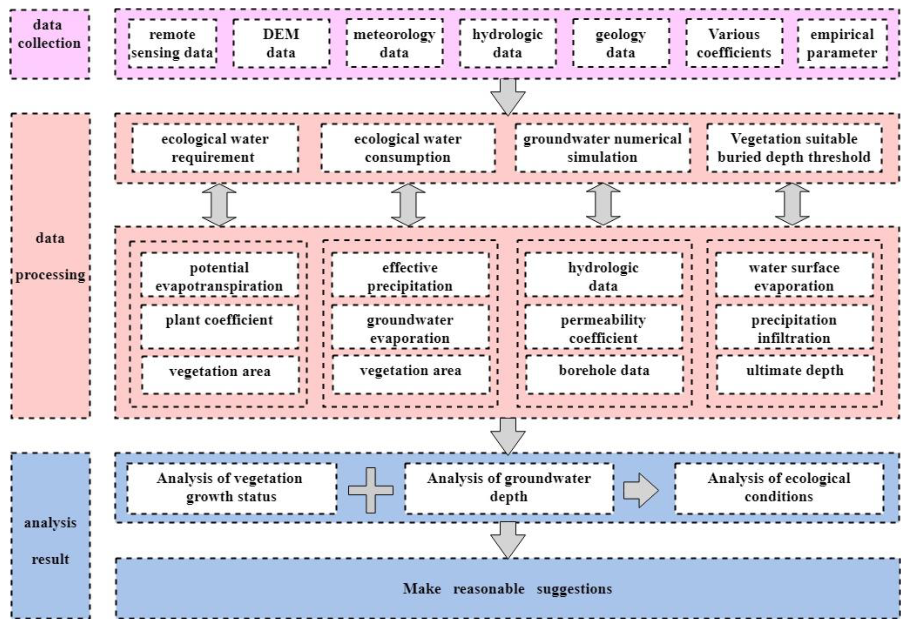
2.2. Research Methods

2.2.1. Crop Evapotranspiration Determination

We calculate crop evapotranspiration using the Penman–Monteith equation recommended by FAO [26]:

$${\mathrm{E}\mathrm{T}}_0=\frac{0.408∆\left({\mathrm{R}}_{\mathrm{n}}-\mathrm{G}\right)+\mathsf{\gamma }\frac{900}{\mathrm{T}+273}{\mathrm{U}}_2\left({\mathrm{e}}_{\mathrm{s}}-{\mathrm{e}}_{\mathrm{a}}\right)}{∆+\mathsf{\gamma }\left(1+0.34{\mathrm{U}}_2\right)}$$

(1)

In Formula (1): ${ET}_0$ is potential evapotranspiration (mm), $R_n$ is the net radiation of crop surface (MJ·m⁻²·d⁻¹), $G$ is the soil heat flux (MJ·m⁻²·d⁻¹), $e_s-e_a$ are saturated vapor pressure and actual vapor pressure, respectively (kpa), $∆$ is the slope of the saturation water vapor pressure curve, $T$ is the average daily temperature (°C), $\gamma$ is the hygroscopic constant, $\gamma$ = 0.066 kpa/°C, $U_2$ is the wind speed at a height of 2 m (m·s⁻¹), and the specific calculation formula of $R_n$ is as follows:

$${\mathrm{R}}_{\mathrm{n}}={\mathrm{R}}_{\mathrm{n}\mathrm{s}}-{\mathrm{R}}_{\mathrm{n}\mathrm{l}}$$

(2)

$$∆=\frac{4098\left[0.6108\mathrm{e}\mathrm{x}\mathrm{p}\left(\frac{17.27\mathrm{T}}{\mathrm{T}+237.3}\right)\right]}{{\left(\mathrm{T}+237.3\right)}^2}$$

(3)

In Equation (2): $R_{ns}$ is net shortwave radiation (MJ·m⁻²·d⁻¹), determined by solar radiation and the number of hours of oral irradiation. $R_{nl}$ is net longwave radiation (MJ·m⁻²·d⁻¹), and it is determined by a combination of the number of hours of oral illumination, the maximum temperature at the mouth, the minimum temperature at the mouth, the altitude, and the actual water vapor pressure. Soil heat flux G has a small value at the mouth-by-mouth scale and is neglected to be 0. The calculation formula at the monthly scale is as follows:

$$\mathrm{G}=0.07({\mathrm{T}}_{\mathrm{i}}-{\mathrm{T}}_{\mathrm{i}-1})$$

(4)

In Equation (4): $T_i$ is the average temperature of month i, and $T_{i-1}$ is the average temperature of month i − 1.

$$\mathsf{\gamma }=0.00163\frac{{\mathrm{p}}_{\mathrm{a}}}{\mathsf{\beta }}$$

(5)

$${\mathrm{e}}_{\mathrm{s}}=\frac{\mathrm{e}{(\mathrm{T}}_{\mathrm{m}\mathrm{a}\mathrm{x}})+\mathrm{e}({\mathrm{T}}_{\mathrm{m}\mathrm{i}\mathrm{n}})}{2}$$

(6)

$$\mathrm{e}{(\mathrm{T}}_{\mathrm{m}\mathrm{a}\mathrm{x}})=0.6108\times \mathrm{e}\mathrm{x}\mathrm{p}\left(\frac{17.27{\mathrm{T}}_{\mathrm{m}\mathrm{a}\mathrm{x}}}{{\mathrm{T}}_{\mathrm{m}\mathrm{a}\mathrm{x}}+237.3}\right)$$

(7)

$${\mathrm{e}}_{\mathrm{a}}={\mathrm{e}}_{\mathrm{s}}\frac{\mathrm{R}{\mathrm{H}}_{\mathrm{m}\mathrm{e}\mathrm{a}\mathrm{n}}}{100}$$

(8)

$${\mathrm{u}}_2={\mathrm{u}}_{\mathrm{s}}\frac{4.87}{\mathrm{l}\mathrm{n}(67.8\mathrm{s}-5.42)}$$

(9)

In the formula above: $p_a$ is the atmospheric pressure (kPa), $\beta$ is the latent heat of vaporization (MJ·kg⁻¹), $T_{max}$ is the average monthly maximum temperature (°C), $T_{min}$ is the average monthly minimum temperature (°C), $R{H}_{mean}$ is the monthly average relative humidity (%), and $u_s$ is the wind speed at a height of sm (m·s⁻¹).

2.2.2. Ecological Water Requirement Calculation of Vegetation

The EWD of vegetation in the study area was calculated using the Penman–Monteith formula recommended by the Food and Agriculture Organization of the United Nations (FAO). This method is a crop development rate assuming ideal soil fertility, moisture, and other conditions [27]. The equation for calculating the evapotranspiration of various types of vegetation is

$$ET=K\times {ET}_0$$

(10)

In Equation (10): $ET$ is vegetation evapotranspiration (mm), $K$ is the crop coefficient, and ${ET}_0$ is crop evapotranspiration.

$$\mathrm{W}={\sum }_{\mathrm{i}}\mathrm{E}\mathrm{T}\times {\mathrm{A}}_{\mathrm{i}}$$

(11)

In Equation (11): $W$ is the ecological water requirement of vegetation (m³) and $A_i$ is the area of vegetation (m²).

2.2.3. Determination of Vegetation Ecological Suitable Water Level Threshold

We choose the diving evaporation model applicable to arid zone conditions, which reflects the relationship between vegetation cover and groundwater burial depth [9]. The calculation formula is

$${\mathrm{H}}_{\mathrm{r}}={\mathrm{H}}_{\mathrm{m}\mathrm{a}\mathrm{x}}\left[1-\sqrt[\mathrm{b}]{({\mathrm{E}}_{\mathrm{r}}-{\mathrm{P}}_{\mathrm{e}})/({\mathrm{E}}_0\times \mathrm{a})}\right]$$

(12)

$$P_e=c\times P$$

(13)

In Equation (13): $H_r$ is the appropriate ecological water level, $H_{max}$ is the buried depth of groundwater, $P_e$ is effective precipitation, $P$ is precipitation, c is rainfall infiltration coefficient, $a$ is the vegetation cover coefficient, taken as 1.174, $b$ is the soil coefficient, taken as 3.63, and $E_0$ is the average evaporation per unit time.

2.2.4. Groundwater Numerical Simulation

We simulate the study area using a finite cell grid, and the model can be described by the differential equation [28]:

$$\left\{\begin{array}{c}\frac{\partial }{{\partial }_{\mathrm{x}}}\left({\mathrm{K}}_{\mathrm{x}}\frac{{\partial }_{\mathrm{h}}}{{\partial }_{\mathrm{x}}}\right)+\frac{\partial }{{\partial }_{\mathrm{y}}}\left({\mathrm{K}}_{\mathrm{y}}\frac{{\partial }_{\mathrm{h}}}{{\partial }_{\mathrm{y}}}\right)+\frac{\partial }{{\partial }_{\mathrm{z}}}+\mathsf{\epsilon }=\mathsf{\mu }\frac{{\partial }_{\mathrm{h}}}{{\partial }_{\mathrm{t}}} \mathrm{x},\mathrm{y}\in \Omega \\ {\mathrm{K}}_{\mathrm{x}}{\left(\frac{{\partial }_{\mathrm{h}}}{{\partial }_{\mathrm{x}}}\right)}^2+{\mathrm{K}}_{\mathrm{y}}{\left(\frac{{\partial }_{\mathrm{h}}}{{\partial }_{\mathrm{y}}}\right)}^2+\mathrm{p}=\mathsf{\mu }\frac{{\partial }_{\mathrm{h}}}{{\partial }_{\mathrm{t}}} \mathrm{x},\mathrm{y}\in \Omega \\ \mathrm{h}\left(\mathrm{x},\mathrm{y}\right){|\mathsf{\Gamma }}_1={\mathrm{h}}_1\left(\mathrm{x},\mathrm{y}\right) \mathrm{x},\mathrm{y}\in {\mathsf{\Gamma }}_1\\ {\mathrm{K}}_{\mathrm{x}}\frac{{\partial }_{\mathrm{h}}}{{\partial }_{\tilde{\mathrm{n}}}}|{\mathsf{\Gamma }}_2=\mathrm{q}\left(\mathrm{x},\mathrm{y}\right) \mathrm{x},\mathrm{y}\in {\mathsf{\Gamma }}_2\end{array}\right.$$

(14)

In Equation (14): Ω is the seepage area, $h$ is the aquifer water level (m), $K$ is the permeability coefficient (m/d), Kn is the boundary surface vertical permeability coefficient (m/d), $\mu$ is the gravity feed degree of the submerged aquifer,$\epsilon$ is the source sink term of aquifer (1/d), $p$ is diving evaporation and rainfall (1/d), ${\Gamma }_1$ is the seepage zone water level boundary, ${\Gamma }_2$ is the seepage zone flow boundary, $\tilde{n}$ is the vertical direction of the boundary surface, $q\left(x,y,z\right)$ is the single wide flow on the class II boundary (m²/dm), the inflow is positive, the outflow is negative, and the impermeability boundary is zero.

2.2.5. Ecological Water Consumption Calculation of Vegetation

Vegetation water consumption refers to the actual water consumption of vegetation, which mainly includes groundwater diving evaporation and soil water storage of precipitation. We calculated the diving evaporation and ecological water consumption intensity according to Avyanov’s diving evaporation model.

$$W_h={\sum }_i{ET}_h{\times A}_i$$

(15)

$${ET}_h=P_e+E_g$$

(16)

$$E_g=\mathrm{a}{(1-\mathrm{H}/H_{max})}^b\times E_0$$

(17)

In the formula above: ${ET}_h$ is the ecological water consumption quota of vegetation, $E_g$ is the groundwater diving evaporation intensity, and $E_0$ is the evaporation intensity of the water surface, expressed by the evaporation amount of E601 evaporator.

2.3. Data Source

According to the study, we collected and organized meteorological, hydrogeological, and elevation data, combined with remote sensing and field survey data for analysis (Figure 2). Precipitation temperature and other weather data were obtained from https://data.cma.cn/data/detail/dataCode/B.0011.0001C.html, accessed on 21 March 2023. Elevation data from https://www.resdc.cn/data.aspx?DATAID=217, accessed on 24 March 2023. Remote sensing data from https://earthexplorer.usgs.gov/, accessed on 21 February 2023. Soil data from https://www.resdc.cn/data.aspx?DATAID=260, accessed on 27 February 2023. Drill hole data from https://zk.cgsi.cn/, accessed on 11 April 2023. Water resource data from http://slt.xinjiang.gov.cn/slt/szygb/list.shtml, accessed on 19 January 2023. And other data come from past scientific surveys and previous studies.

3. Results

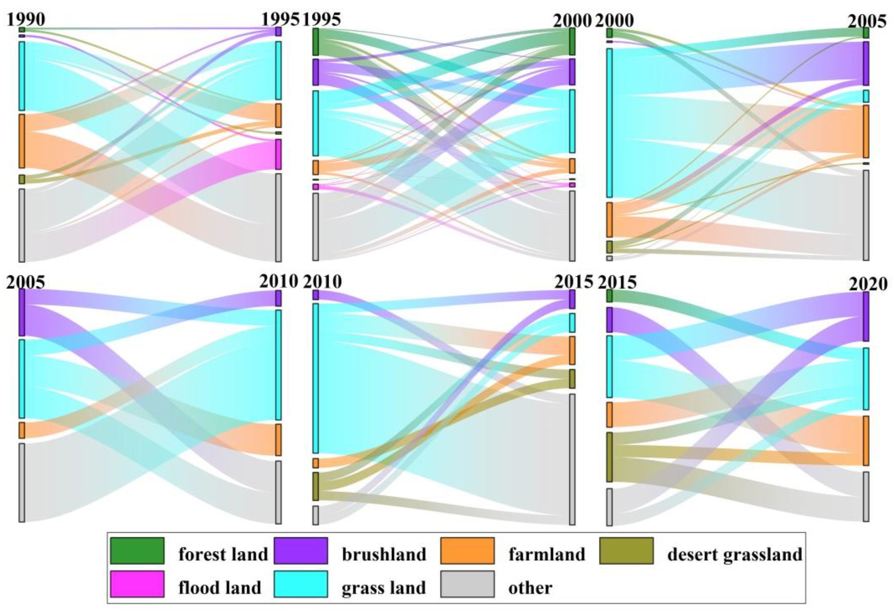
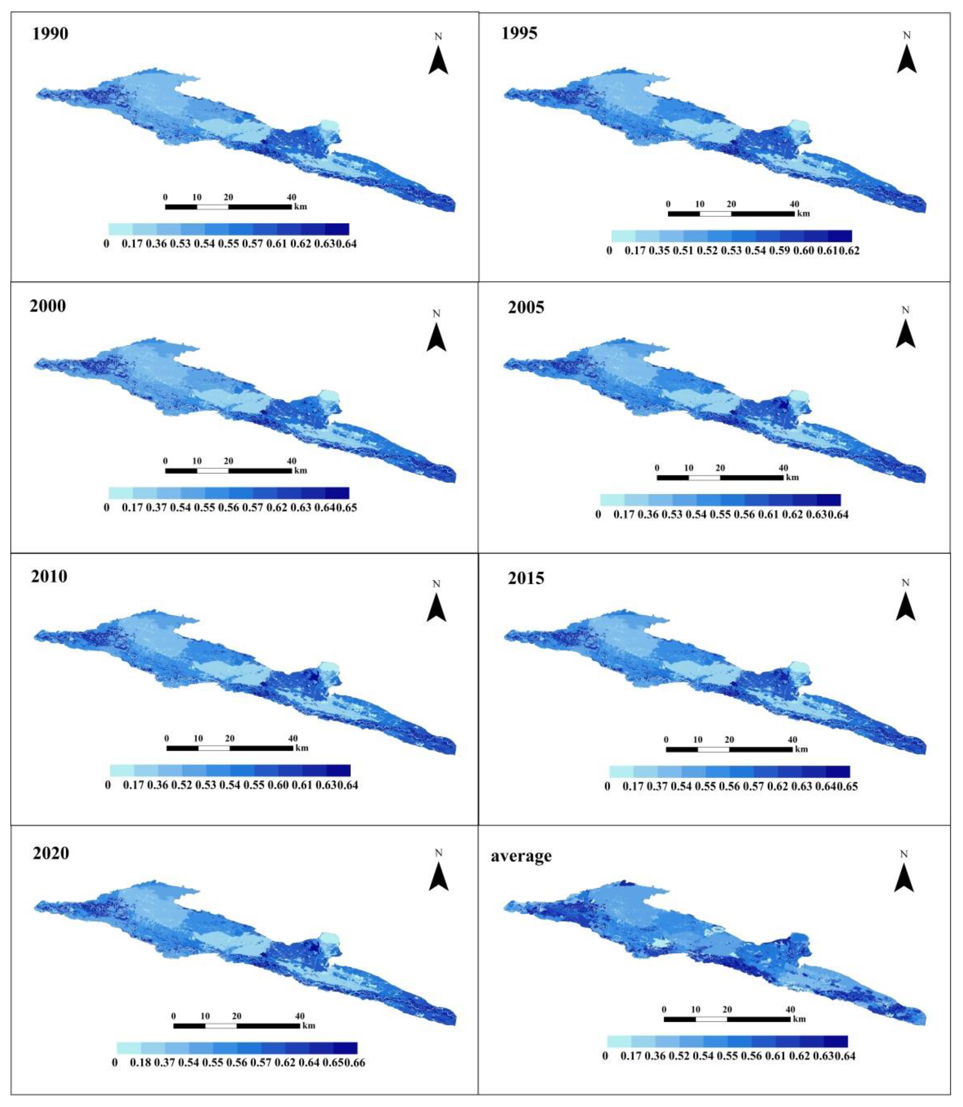
3.1. Vegetation Coefficient and Vegetation Distribution

The study area is located in a typical arid region of China, where precipitation is scarce but evapotranspiration is high, about six times the amount of precipitation. Between 1990 and 2020, precipitation showed a trend of dynamic equilibrium, and the potential evapotranspiration showed a trend of slow increase, especially after 1995. This also affects the changes in the ecological water demand of vegetation (Figure 3).

The vegetation coefficient is the ratio between the potential water demand of the vegetation and the potential evapotranspiration. It can vary depending on the type of vegetation, different growth stages of the same vegetation, and the month of the year. The vegetation growth cycle can be divided into four stages: initial, development, mid-season, and late season. For the month selection, we can focus on the main growing period of vegetation in arid regions, which typically spans from April to October. Due to the sparse vegetation in arid regions, the vegetation coefficient is primarily influenced by leaf area index (LAI) and coverage [29,30]. Based on the recommendations of FAO, we determined the vegetation coefficients for different vegetation types and different months in the research area (

Table 1. Different monthly coefficients of various vegetation types.

Month	Forest Land	Brushland	Grassland	Desert Grassland	Farmland	Flood Land
4	0.5	0.3	0.4	0.1	0.4	0.2
5	0.7	0.4	0.6	0.2	0.6	0.3
6	0.9	0.5	0.8	0.25	0.8	0.35
7	1.1	0.6	0.9	0.3	0.9	0.4
8	0.8	0.5	0.8	0.25	0.8	0.35
9	0.6	0.4	0.6	0.2	0.6	0.3
10	0.5	0.3	0.4	0.1	0.4	0.2

).

In the study area, the vegetation is mainly distributed along the river banks and consists mainly of forests and grasslands, with a mixture of forested areas and grassland patches. The forests are composed of deciduous trees and understory shrubs, including poplar, birch, willow shrubs, and wild hawthorn, among others. The grasslands consist mainly of reeds, bitter vetch, and Artemisia species vegetation. In the cultivated areas, corn is the predominant crop.

We used an object-oriented remote sensing classification method to interpret the Landsat TM remote sensing data in the study area. The Normalized Difference Vegetation Index (NDVI) and Mahalanobis distance methods were used to detect and classify different vegetation patches within the study area [31]; land use in the study area was classified into six categories: woodland, shrubland, grassland, desert grassland, cultivated land, and riparian land (Figure 4). The vegetation in the area is mainly composed of grasslands, which occupy about half of the total study area. Most of the grasslands are distributed in the wetlands downstream of the river valley, while the rest are found around the forested areas [32]. The second largest land cover category is shrubland, followed by cropland. Cultivated land is primarily distributed in the upstream areas of the study area, where human development occurred earlier. Scrubland is also distributed in the central part of the research area, acting as a transitional zone between forests and grasslands. Forested land occupies only 11.36% of the total research area, with the majority distributed along the banks of the river.

In the last 30 years, the forest area in the river valley area has increased, mainly concentrated in the period from 1995 to 2005, but the rate of increase is slow, and the new area accounts for only about 4% of the total forest area. Shrubland has also experienced slow growth, primarily concentrated between 1995 and 2000, with an additional area of approximately 7.29 × 10⁷ m². The area of grassland and desert grassland decreased, mainly to cropland and other land. The area of beach land increased slightly, but remained stable overall. Cultivated land increased more, accounting for about 13% of the total cultivated land, mainly concentrated in the period from 1990 to 2005 (Figure 5).

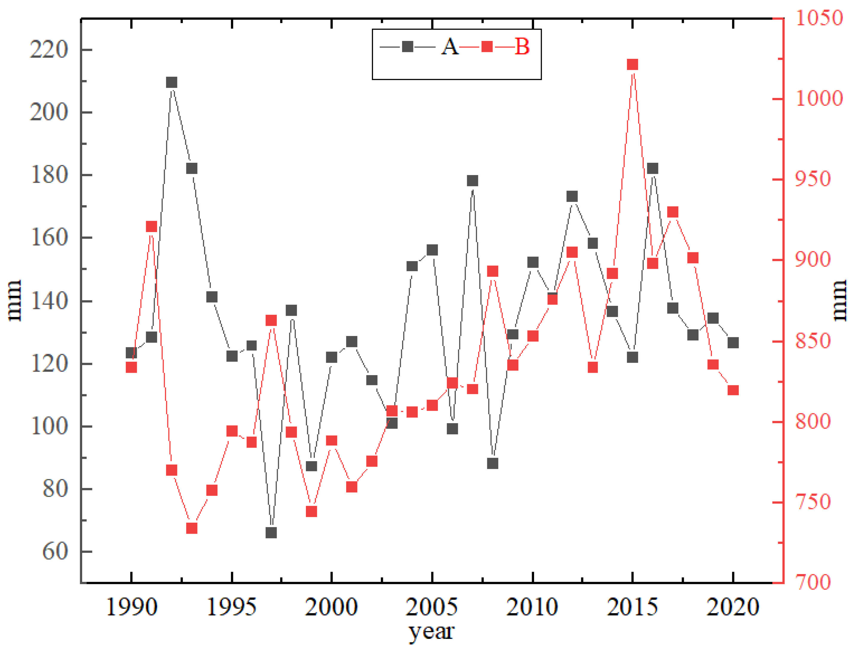
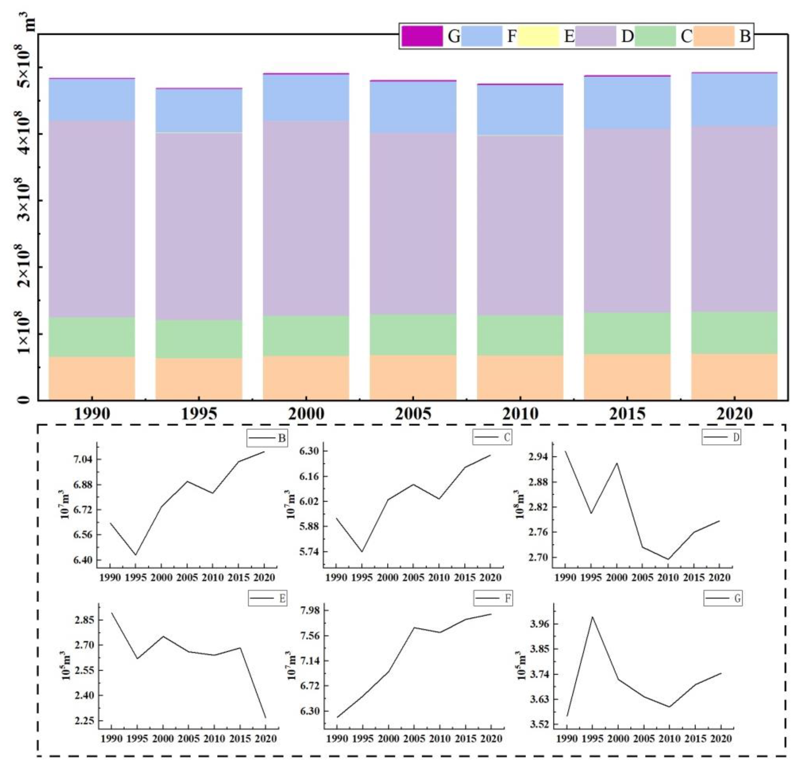
3.2. Ecological Water Requirement Analysis of Vegetation

According to the above vegetation ecological water demand formula, we calculate the water demand quota of all kinds of vegetation in the study area from 1990 to 2020, five years by five years. The results show that among all types of vegetation, the water demand rate of forest land is the largest, followed by grassland and cultivated land, and the ecological water demand rate of desert grassland and river beach land is smaller (

Table 2. The average monthly water requirement quota of all kinds of vegetation for many years (mm).

Annual Average	Forest Land	Brushland	Grassland	Desert Grassland	Farmland	Flood Land
4	42.89	26.12	33.65	8.21	34.56	17.49
5	92.45	53.54	77.65	25.24	79.57	40.27
6	145.77	81.92	126.88	38.66	130.05	57.68
7	154.31	85.40	123.69	39.87	126.43	56.49
8	92.93	58.92	90.99	27.47	93.078	40.88
9	44.52	30.08	43.63	14.13	44.71	22.55
10	18.80	11.44	14.75	3.61	15.13	7.58

). During the period from April to October, the ecological water demand quota in July is the largest, followed by June and August, and the smallest is in October.

In the last 30 years, the ecological water demand of all types of vegetation in the valley area has changed little and appears to be relatively stable overall, influenced mainly by potential evapotranspiration [33,34]. The areas with high ecological water demand quota are mainly concentrated in the upstream and downstream wetlands of the study area, as well as the areas through which rivers flow. The areas with low water demand ratio are mainly concentrated in desert grassland and desert shrubland in the middle of the study area, and the change of water demand ratio is mainly cultivated land and grassland (Figure 6).

According to the above vegetation area and crop ecological water demand quota, the ecological water demand of the study area from April to October in the past 30 years was calculated. The results showed that the water requirement of vegetation in the valley did not change much, and it slowly increased after 1995, and the overall stability was about 4.82 × 10⁸ m³. The water demand in the lower reaches of the wetland and the upper reaches of the grassland in the study area is more concentrated, and the ecological water demand in the middle reaches is less. In 2000, the water demand of the downstream wetland remained stable after the change, and the water demand in the middle reaches changed the most. Among the different vegetation types, grassland ecosystems have the highest water demand, accounting for about half of the total water demand. This is followed by croplands and forests, while desert grasslands and riparian zones have the lowest water demand. Over the past 30 years, forested areas, shrublands, and cultivated land have shown a fluctuating upward trend in water demand, while grasslands, desert grasslands, and riparian zones have exhibited a declining trend. Among them, grasslands and cultivated land have experienced the most significant changes (Figure 7). The highest ecological water demand occurs in July each year, while the lowest water demand is observed in April and October.

3.3. Vegetation Suitable Buried Depth Threshold

The appropriate ecological burial depth refers to the ideal groundwater level at which various types of vegetation can meet their growth requirements. It is influenced by multiple factors. We determine the suitable underground water depth for each type of vegetation based on the ratio between actual water demand and potential evapotranspiration. According to previous research, vegetation can maintain normal growth when its water consumption reaches 70% of the water demand [35].

Before calculating the ecological burial depth, it is necessary to obtain the monthly effective precipitation over the past 30 years in the study area based on precipitation data. In arid regions, effective precipitation is particularly important. Generally, it is considered that when rainfall exceeds 50 mm, the precipitation coefficient is set to 0.8. For rainfall between 5–50 mm, the precipitation coefficient is set to 1. When rainfall is less than 5 mm, the precipitation coefficient is set to 0 [36]. We use the Averyanov evapotranspiration model to inversely determine the appropriate ecological burial depth for vegetation. According to previous research, in vegetated areas, the maximum groundwater burial depth is generally between 3.5–6 m. Let us assume a maximum burial depth of 6 m. For the Averyanov model, we can use a value of 1.174 for parameter a and 3.63 for parameter b [9,37]. To estimate the water surface evaporation intensity, we can use the annual evaporation measured in millimeters from the 20 cm evaporation pan at the hydrological station. Let us consider the average evaporation value over a period of 30 years (

Table 3. Average evaporation for many years (mm).

Month	4	5	6	7	8	9	10
Evaporation capacity	99.64	156.61	159.82	154.21	139.08	112	59.17

).

The results indicate that forested areas have the smallest threshold for suitable burial depth among various types of vegetation in the study area, with an average annual burial depth of 2.06 m. Grasslands and cultivated land come next, with a relatively small difference between them. Desert grassland has the largest suitable burial depth, with an average annual depth of around 3.9 m (Figure 8). Over the course of a year, the suitable ecological burial depth is smaller in June and July, while it is larger in April and October. The main reason for this is the higher temperatures and greater evaporation during June and July, coupled with scarce precipitation in arid regions. Vegetation requires more water from the groundwater to support its growth during these months. Therefore, the ideal underground water level should be relatively shallow during this period to ensure sufficient water availability for the plants.

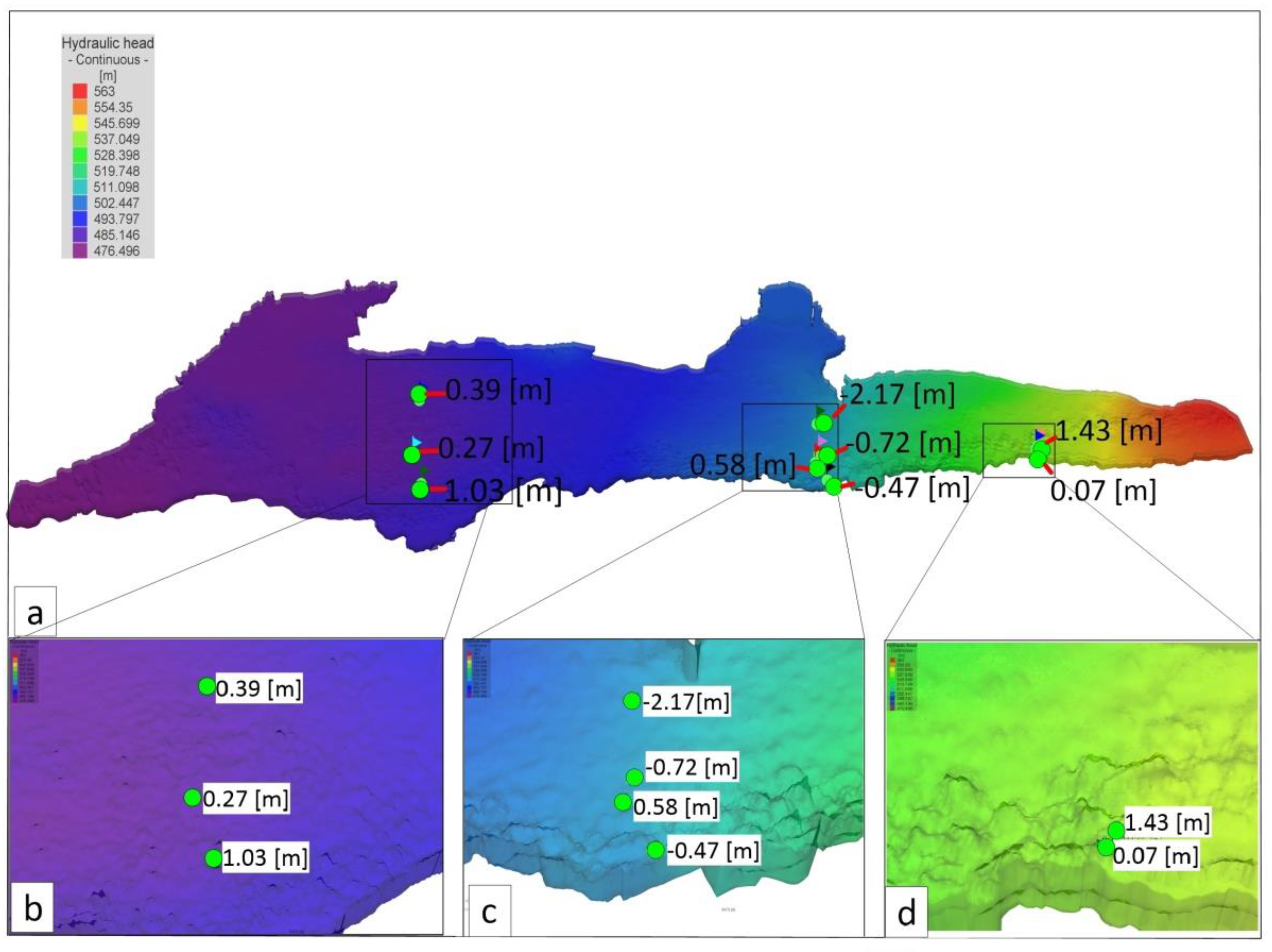
3.4. Groundwater Numerical Simulation

Based on the geological conditions and hydrological data of the study area, as well as considering meteorological factors, elevation, and corresponding parameters, we conducted groundwater simulation. The study area was divided into 7.83 × 10⁵ triangular mesh grids using a three-dimensional approach. The density of grid cells was increased by 15 times near river areas to capture the dynamics of water flow more accurately. This process resulted in the construction of a comprehensive three-dimensional numerical model for groundwater in the study area (Figure 9). We designated the period from January 2014 to January 2015 as the validation period for the model. During this time, we imported data from nine groundwater monitoring wells within the study area. To assess the accuracy of the model, a tolerance of 2 m was set for comparing the simulated water levels with the observed values from these wells. The results indicate that the water levels in eight out of the nine monitoring wells are within the defined error range, while one well is slightly beyond the tolerance. The current model is well fitted and can predict the impact of the construction of water projects in the upstream area on groundwater changes.

Based on the successful model validation during the verification period, we can proceed to simulate the groundwater levels and their changes according to the water resource planning for the study area. By using the model, we obtained the simulated groundwater level conditions within the study area from 1990 to 2020, providing insight into the groundwater dynamics over this timeframe (Figure 10. The research indicates that over the past 30 years, the groundwater levels in the river valley area have shown a slow declining trend, with a cumulative decrease of approximately 27 cm. From 1990 to 2000, the groundwater levels remained relatively stable overall and showed a slight increasing trend. However, after the construction of water conservancy projects such as dams and regional water transfers in the upstream area in 2000, the groundwater level in the study area declined more significantly, with an average annual decline of 1.3 cm. Among these trends, the influence of rivers on groundwater recharge is evident. Areas near the river experience a slower decline in groundwater levels compared to areas farther from the river. The rate of groundwater level decline in areas away from the river is about twice that of areas near the river. From January to April, the groundwater levels remain relatively stable. However, starting from May, a decline in groundwater levels becomes noticeable. During the inundation and irrigation of the river valley in June, artificial flooding was created using hydraulic works and the water level appeared to rise. However, as temperatures increase and evaporation rates rise, the groundwater levels continue to decline, exhibiting an overall fluctuating downward trend.

According to the groundwater level from 1990 to 2020, combined with the DEM data of the study area, the groundwater depth in the study area was obtained (Figure 11). The results show that the groundwater level in the study area has been slowly decreasing and the depth of groundwater is becoming deeper and deeper since 30 years due to the local hydraulic projects. This trend is particularly evident in the central and upstream areas of the river valley, which are farther away from the river. In contrast, the downstream wetland areas have the shallowest groundwater depths. The changes in groundwater depth are mainly concentrated in the middle section of the river valley. In two-thirds of the study area, there is an increase in groundwater depth, but the magnitude of the increase is relatively small. This increase is primarily concentrated in the middle section of the river valley and some upstream areas, with the majority of increases being less than 0.5 m. However, the downstream areas of the river valley experience a decrease in groundwater depth, with the decline ranging from 0 to 0.6 m.

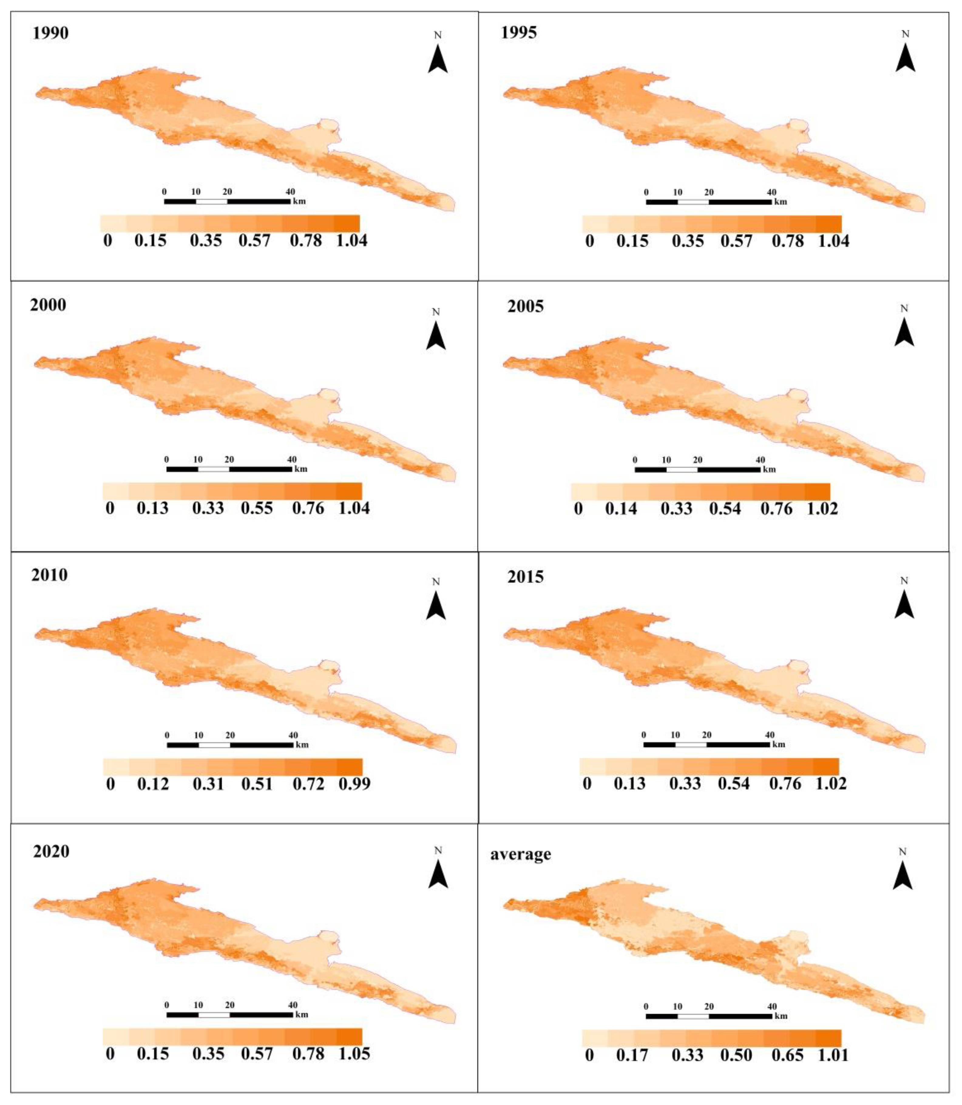
3.5. Ecological Water Consumption Analysis of Vegetation

Based on the Averyanov groundwater evaporation model, combined with the results of groundwater depth, we calculated the groundwater evaporation and ecological water consumption quota of the study area from 1990 to 2020 (Figure 12). According to previous studies and empirical parameters, the limit burial depth of the study area is 6 m, and the coefficients a and b are 1.174 and 3.63, respectively [38,39]. The results indicate that forested areas and riparian zones in the study area have the highest annual water consumption quotas, followed by grasslands and cultivated land. Shrublands and desert grasslands have relatively smaller water consumption quotas. The vegetation consumes the most water in June, followed by July and May, and the vegetation consumes the least water in October.

Among the vegetation in the study area, the ecological water consumption of grassland is the largest, followed by that of forest land and shrubland, and the water consumption of desert grassland is the smallest. The interannual variation of ecological water consumption is consistent with the ecological water consumption quota. The higher water consumption is mainly concentrated in the wetland in the lower reaches of the valley and the cultivated land and grassland in the upper reaches. The decline in groundwater levels over the past 30 years has also led to an overall slow downward trend in ecological water consumption by vegetation in the study area, reaching a minimum in 2010 (Figure 13). The water consumption in the downstream region remained relatively stable with minimal changes, while the central region experienced more pronounced variations in water consumption. In the river valley area, except for grasslands, all other types of vegetation showed a declining trend in ecological water consumption, with shrublands and desert grasslands showing particularly significant decreases. Forested areas experienced a slower decline, while grasslands exhibited dynamic fluctuations in water consumption.

3.6. Analysis of Ecological Conditions

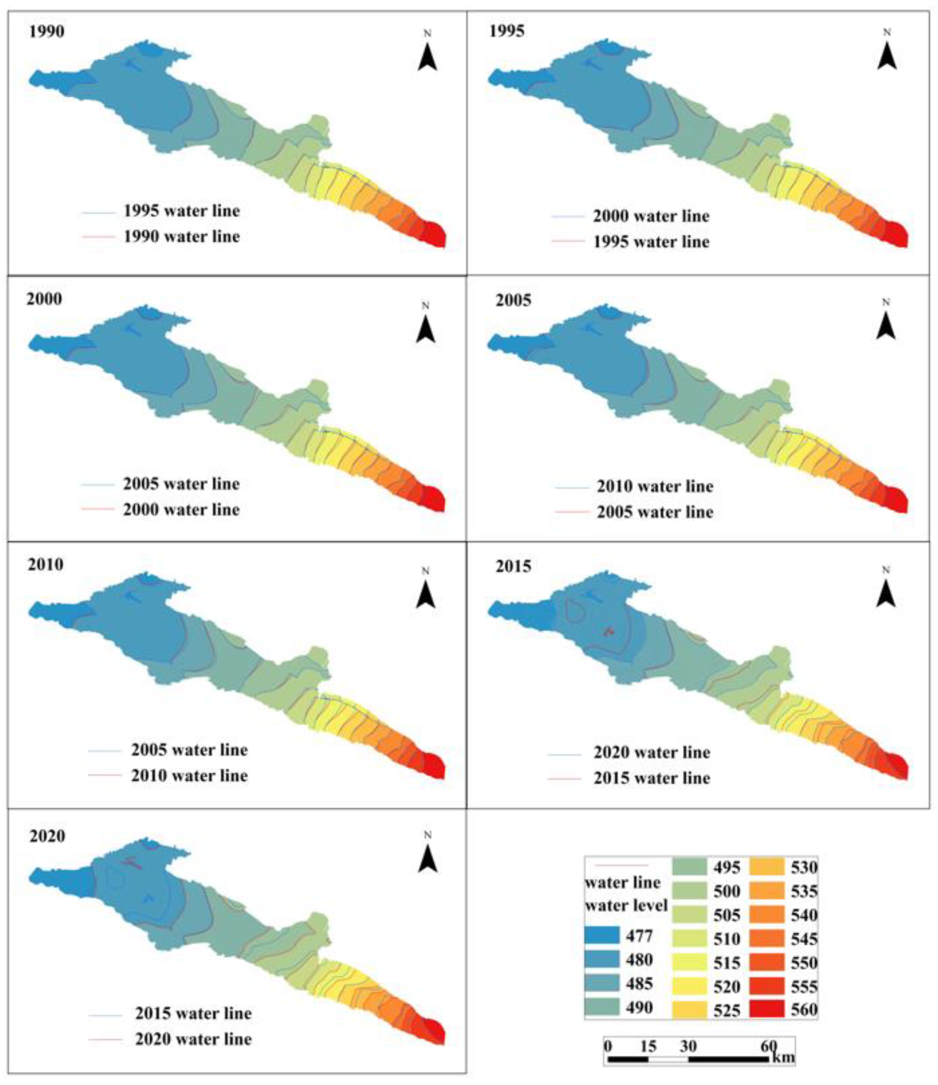
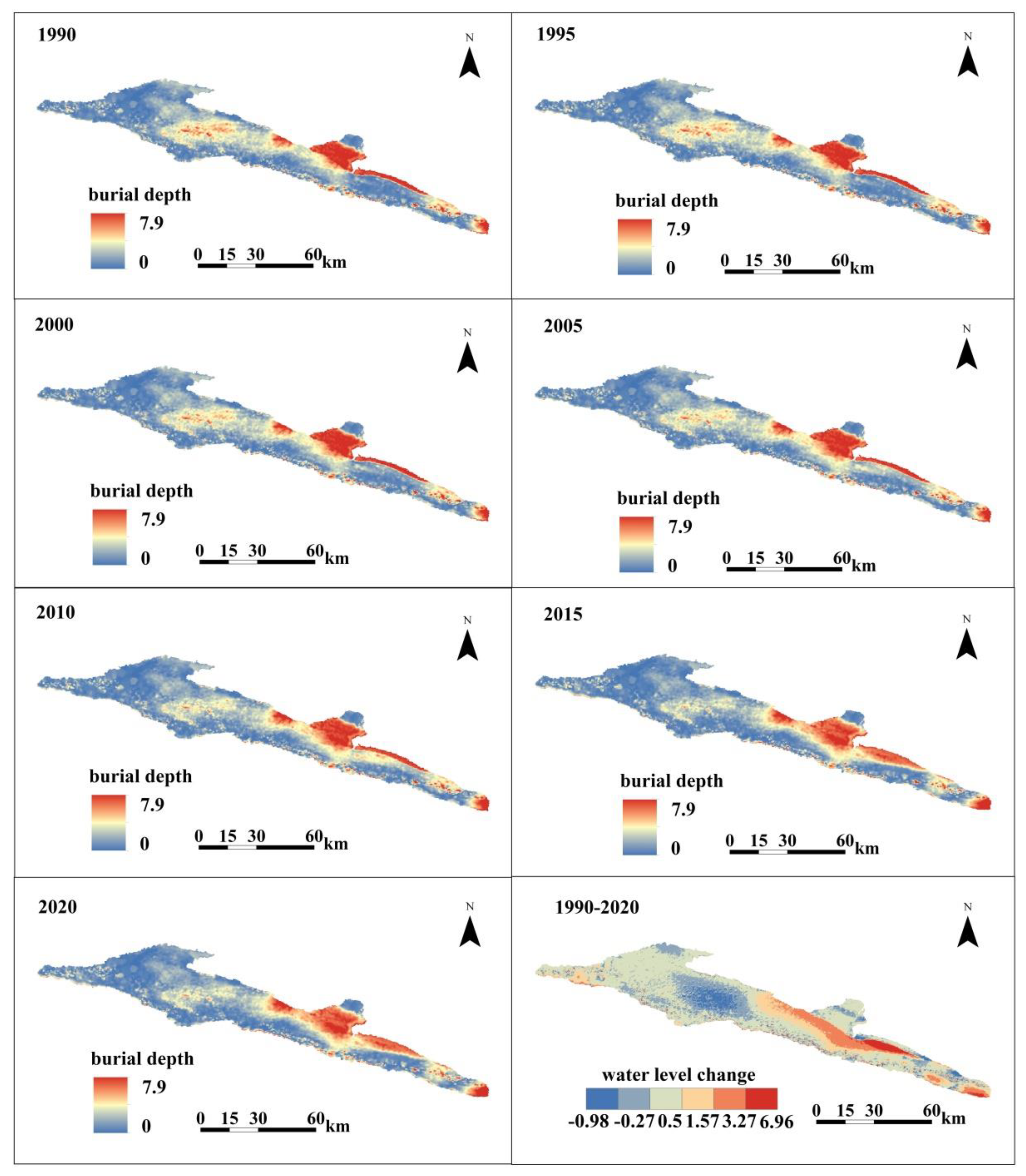
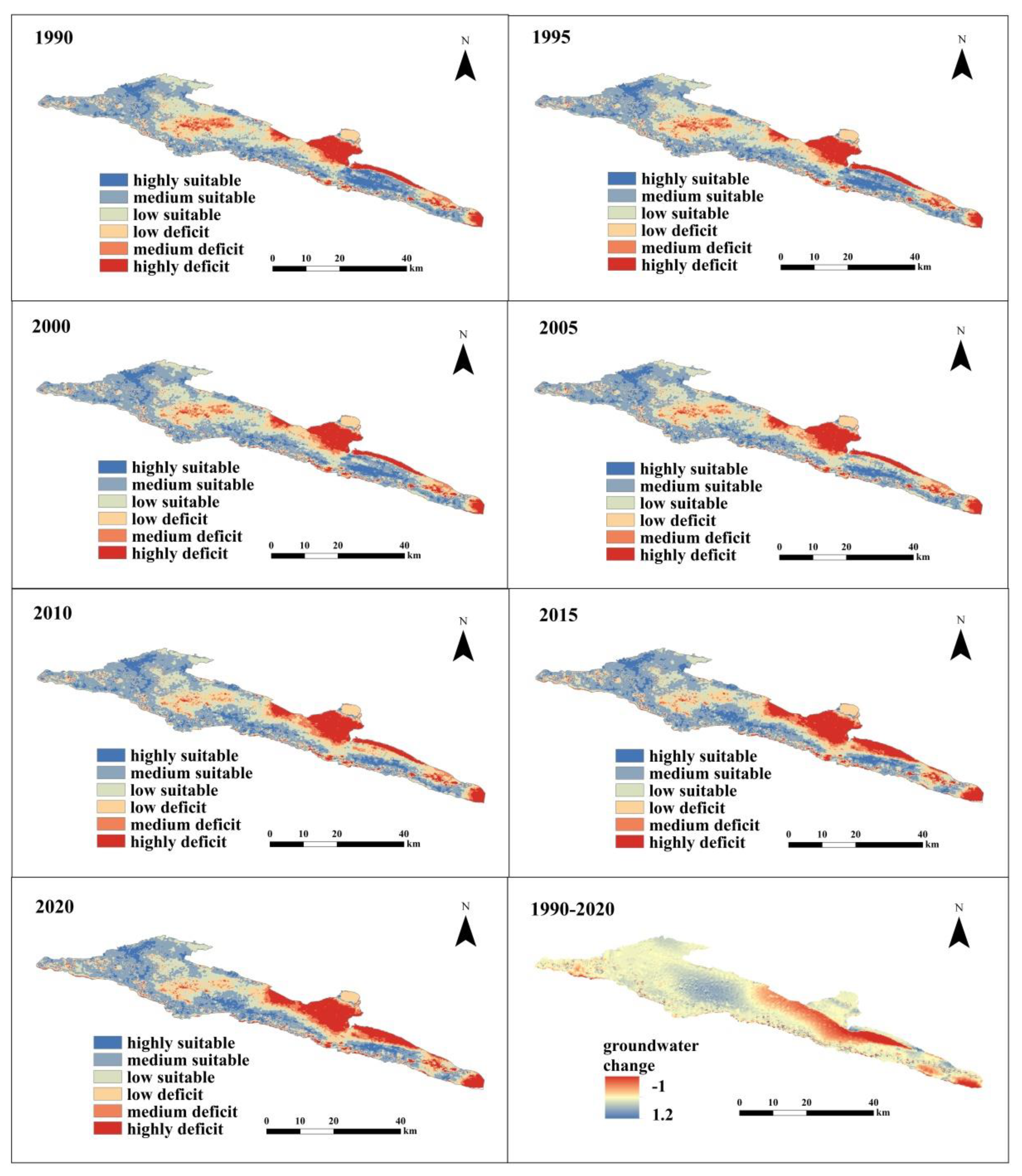
3.6.1. Analysis of Groundwater Condition

Groundwater is the main source of water for vegetation growth in arid areas. According to the measured and predicted groundwater level, combined with the suitable groundwater level depth of vegetation, we obtained the groundwater status data from 1990 to 2020 (Figure 14). Combined with previous studies to establish groundwater evaluation levels, the groundwater condition of the study area was divided into six levels, and groundwater ecological safety analysis was conducted for the study area (

Table 4. Groundwater status grade (m).

Grade	Highly Suitable	Medium Suitable	Low Suitable	Low Deficit	Medium Deficit	Highly Deficit
Burial depth	≤−2	−2–−1	−1–0	0–1	1–2	≥2

).

The results show that the area of groundwater suitable area in the study area accounts for a large proportion, with an average annual proportion of about 65%, of which the area of medium suitable area is the largest, with an average annual proportion of about 35%. The second is low suitable and low deficit areas, with an average annual proportion of 21% and 12%, respectively. The areas with high and medium ecological suitability of groundwater are mainly distributed on both sides of the river and the wetlands in the west of the valley. In these areas, the groundwater level is close to the surface elevation. The areas with low suitability are mainly concentrated near the waters. The deficit areas are primarily distributed in the central and northern highlands of the study area, with the highest deficit areas located in the northern region. In these areas, the elevation is relatively higher, and there is exposure of bedrock, resulting in deeper groundwater depths.

Over the past 30 years, groundwater conditions in the river valley area have gradually deteriorated. From 1990 to 2000, there were relatively small changes in the overall groundwater condition. However, since 2000, there have been more significant fluctuations in groundwater condition. From an overall perspective, the area of groundwater deficit has increased from 31% to 37%, while the corresponding suitable areas have decreased (Figure 15). From the perspective of different suitability levels, all categories of suitable areas have experienced varying degrees of reduction, with low suitability and high suitability areas experiencing the most significant declines. However, there has also been an increase in deficit areas at each level, with the highest deficit areas showing the largest increase in terms of area.

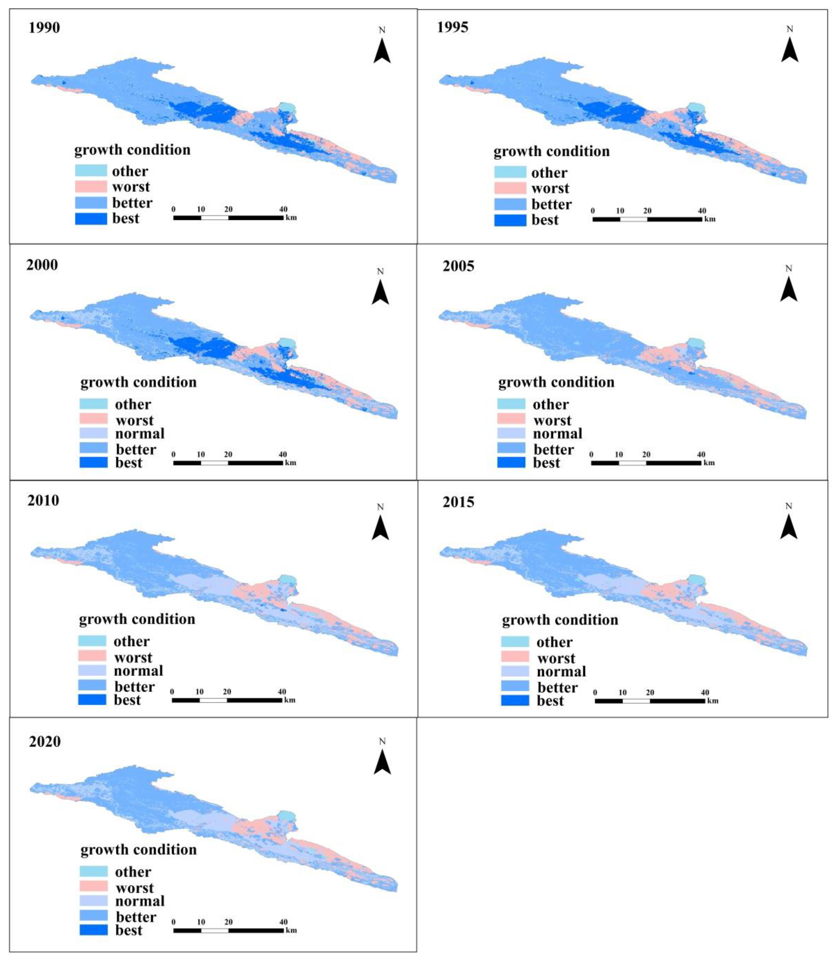
3.6.2. Analysis of Vegetation Growth Status

The growth status of vegetation is the most intuitive indicator of ecological security. Water resources severely limit vegetation growth in arid areas, and changes in groundwater also affect the water use of different types of vegetation. According to the actual situation of the study area, combined with previous studies, we use the ratio of vegetation ecological water consumption and ecological water demand to evaluate the growth of vegetation (

Table 5. Vegetation growth status grade.

Grade	Water Consumption to Water Demand Ratio (%)	Ecological Significance
Worst	<60	Survival constrained
Bad	60–70	Growth is curbed
Normal	70–80	Maintain normal growth
Better	80–90	Growth conditions are good
Best	90–100	The best condition for growth

) [40]. The vegetation growth status was divided into five grades, and the distribution of vegetation growth status in the study area from 1990 to 2020 was obtained (Figure 16).

The results indicate that the total annual vegetation consumption to demand ratio in the study area has gradually decreased from 80% in 1990 to 74% in 2020. The vegetation growth status has shifted from good to maintaining normal growth, with the largest decline observed between 2005 and 2010. Among the different vegetation types, the growth condition of tidelands and grasslands is relatively good and stable. Shrubland and desert grassland have undergone the most significant changes, from optimal growth in 1990 to maintaining normal growth conditions in 2020. Cultivated land is in the worst growth condition, with long-term water shortages affecting its growth. Forests have also moved from good growth to maintaining normal growth.

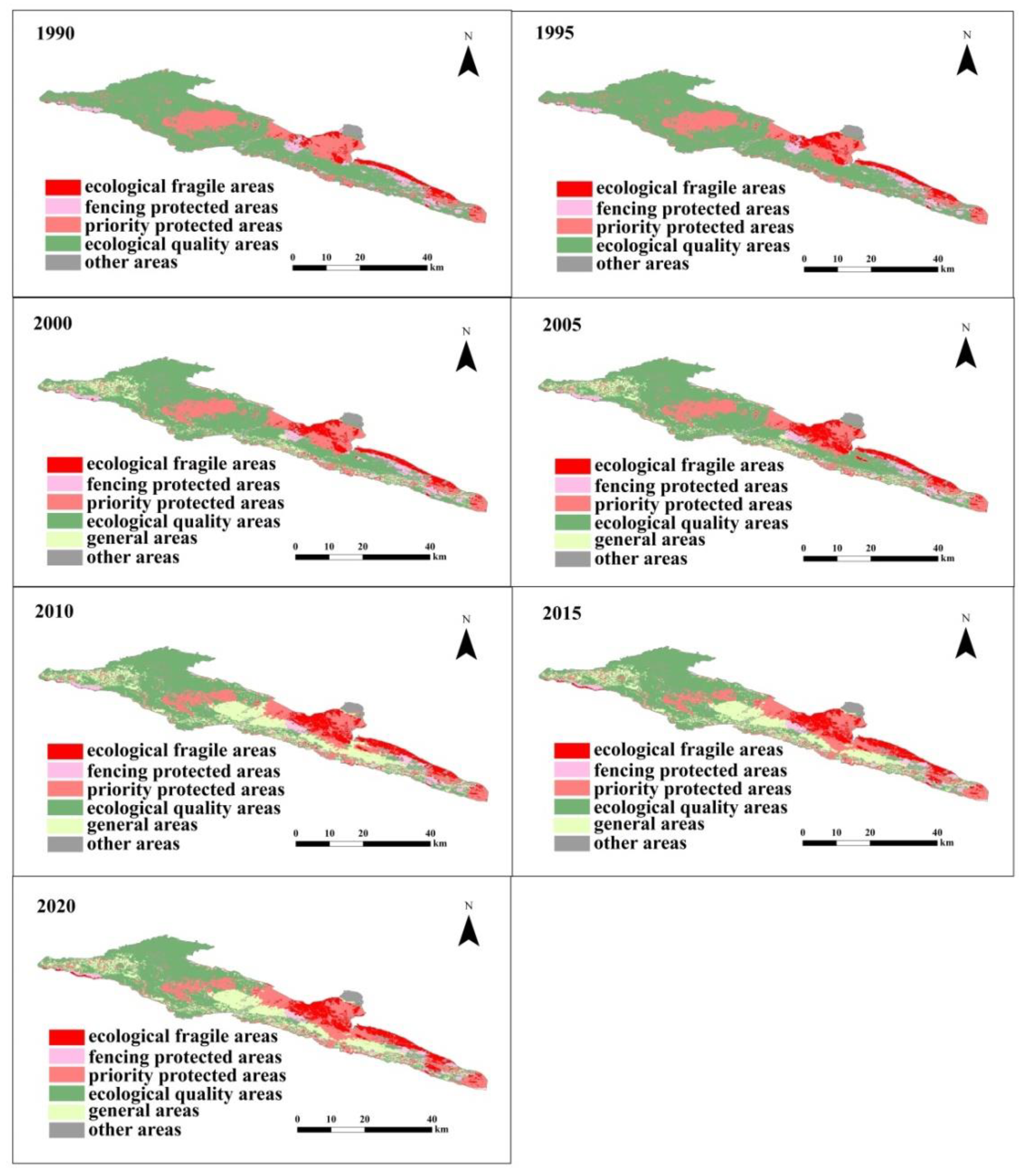
3.6.3. Analysis of Ecological Conditions

Based on the previous analysis of groundwater conditions and vegetation growth in the study area, we combine both factors to assess the ecological security status of the vegetation. We classify the area into six categories: ecological quality areas, ecologically fragile areas, fencing protected areas, priority protected areas, general areas, and other areas (Figure 17).

We classify the areas with suitable groundwater depths and good vegetation growth as ecological quality areas, located mainly downstream and near the middle reaches of the river valleys. We classify the areas with low groundwater depths and limited vegetation growth as ecologically fragile areas, located primarily in the middle reaches of river valleys and away from main watercourses. We classify the areas with suitable groundwater depths but poor vegetation growth as fencing protected areas, located primarily in areas adjacent to overdeveloped rivers. We classify the areas with poor groundwater depths but good vegetation growth as priority conservation areas, located primarily in the northern parts of river valleys and in areas downstream with higher elevations. We classify areas with suitable groundwater depths and normal vegetation growth as general areas, primarily located near rivers. We classify rivers, lakes, and other similar features as other areas.

Over the past 30 years, the area of ecological quality areas has decreased significantly. It has decreased from about 60% of the study area in 1990 to 40% in 2020. The decline has been particularly pronounced since 2010, with the majority of these areas transitioning to general areas. The area of ecologically fragile areas has increased steadily, from 5% to 10%. The area of priority protected areas has remained relatively stable. The area of fencing protected areas has been slowly decreasing, with its proportion decreasing from 5.8% to 3.8%.

4. Discussion

4.1. Estimation of Water Deficiency of Vegetation

The quantitative study of vegetation water requirements has always been of great concern to experts and scholars, especially in arid and semiarid regions. This is also closely related to the ecological issues in mountain-front valleys [10]. The methods for calculating vegetation water requirements may vary, and among them, the approach of determining vegetation ecological quotas based on the Penman formula is more popularly adopted [41,42,43,44]. By applying the Penman formula, we made estimations of vegetation water requirements in the study area. The results, in terms of water demand quotas, are found to be consistent with previous research conducted in this field [45,46]. In the study area, vegetation water requirements are primarily concentrated from April to October each year. Among these months, the water demand during the growing season in June to August is particularly high, accounting for approximately 68% of the total annual water requirements.

Estimation of water scarcity is an important basis for water resources management. The water shortage of vegetation is affected by many factors, such as precipitation, water diversion, and climate. In the past, most of the studies on water scarcity were based on the vegetation water demand minus the effective precipitation, and then the vegetation water scarcity was obtained, which was only a potential water scarcity [47]. Based on the simulated groundwater depth conditions in the study area, we obtained the actual water consumption of vegetation both above and below the ground. By considering the vegetation growth situation, we determined that when the ratio of water consumption to demand reaches 90%, it indicates that all vegetation is growing well. Finally, the required water consumption is subtracted from the actual water consumption to obtain the actual water shortage of vegetation. In the past 30 years, with the decline of groundwater level, the annual vegetation water shortage in the study area has gradually increased from 5.31 × 10⁷ m³ to 7.78 × 10⁷ m³. However, due to the lack of meteorological observation stations in the study area and the lack of hydrogeological data, it will inevitably affect the estimation of ecological water demand.

4.2. Influence of Groundwater Level Change

With the increase of water for industrial production and urban life, the exploitation of groundwater is also increasing, and the construction of water conservancy projects in the upstream areas and the transfer of water from rivers to the outside will lead to the decline of the groundwater level. The factors such as water transfer from rivers will lead to the decline of the groundwater level [48]. The lowering of the groundwater level not only brings the ecological crisis of water resources to the valley, but also directly affects the growth of local vegetation. The coverage and density of vegetation will decrease [49,50]. The simulation prediction shows that after the construction of the upstream water conservancy project, the depth of groundwater in the study area is slowly decreasing, especially since 2000, about 1.3 cm per year, which is similar to the results of the previous study [25,46]. Affected by the decline in groundwater level, the depth of groundwater is becoming deeper and deeper, especially in the central part of the valley far from the river, and the rate of groundwater decline is about twice as fast as that near the river. This also leads to the phenomenon of dry trees and grassland degradation in some areas of the valley [51]. In the next 15 years, the impacts of water projects will continue to intensify, with the area of unsuitable groundwater depth areas increasing by 5.85%. If the average groundwater depth of the valley decreases to 3 m, the area of the deficit area will be about 78% of the study area, which will bring more problems to urban development and ecological safety. Scholars will be concerned with the length of the model validation period, the number of observation wells, and their error range to improve the authenticity of the results and make more scientific proposals.

4.3. Response to Water Ecological Imbalance

Water scarcity is an important factor in the ecological security problems of pre-mountain valleys in arid regions, and open-source flow reduction is the major direction to alleviate the water–ecological imbalance. Inter-regional water transfer can greatly alleviate regional water resource problems, and seepage along the route also recharges groundwater. After we simulated the recharge of the depleted stream channel in the central part of the study area, the groundwater level in the area increased significantly, and the ecologically buried depth of the suitable area increased by 3.56%, which will also better promote the growth of vegetation. According to our analysis of monthly water demand and consumption, June–August is the time when vegetation grows and consumes the most water, and it is the best time for water replenishment, so we suggest that the management department replenish the vegetation in this time period every year, especially increasing the number and length of roaming irrigation for the vegetation [9].

Combining the vegetation growth condition and the groundwater condition in the study area, we analyzed the six different ecological conditions and propose reasonable measures. The vegetation growth in the priority reserve is good, but the groundwater condition is poor, and we suggest focusing on recharging the priority reserve to prevent further degradation of the vegetation. It is recommended that artificial planting be carried out in the closed protection zones, especially in the locally dominant species such as poplar and willow, in order to increase the area of green space, a measure that has also been carried out locally. Continuing to strengthen the protection of ecologically high-quality areas, increasing the area with good vegetation growth and suitable groundwater conditions, and improving the ecological conditions in ecologically fragile areas will improve the quality of habitats in the entire river valley area [52]. In addition, we need to improve the efficiency of water use, optimize the industrial structure, and implement drip or sprinkler irrigation measures in pastoral grasslands. We need to educate local production personnel about scientific water use and raise their awareness of water conservation, so as to promote ecologically sustainable development in arid river valley areas [21].

5. Conclusions

We extracted land cover types through remote sensing data and field survey, and then calculated the ecological water demand and ecological water consumption of vegetation. Combined with the analysis of groundwater numerical simulation water level, the ecological security of the study area was evaluated from the two aspects of river valley groundwater status and vegetation growth status. The main results are as follows:

(1) In the past 30 years, the water demand of vegetation in the valley has not changed much; it has been slowly increasing after decreasing in 1995, and the overall stability is about 4.82 × 10⁸ m³. The water demand of downstream wetlands and upstream grasslands in the study area is more concentrated. Among all kinds of vegetation, the ecological water demand of grassland is the largest, accounting for about half of the total water demand, followed by cultivated land and forest land, and the water demand of desert grassland and flood land is the smallest. Ecological water demand is highest in July, lowest in April and October, and accounts for about 68% of annual water demand from June to August.

(2) During the last 30 years, the construction of water conservancy projects in the upstream area has led to a slow downward trend in the groundwater level in the valley area, with a cumulative decline of about 27 cm. From 2000 to 2020, the decline is more obvious, with an average annual decline of 1.3 cm, and the rate of decline of groundwater level in areas far from rivers is about twice that of river areas. The groundwater level is basically unchanged from January to April each year, and begins to decline in May. During the flood irrigation in the valley in June, the water level increased. Then, with the increase in temperature and evaporation, the water level continued to decline, showing a fluctuating downward trend.

(3) The area of suitable groundwater area in the study area is relatively large, the average annual proportion is about 65%, the area of medium suitable area is the largest, and the average annual proportion is about 35%. The high and medium suitable areas of groundwater ecology are mainly distributed on both sides of the river and the wetland in the west of the valley, and the deficit areas are mainly distributed in the central and northern highlands of the study area. Over the past 30 years, as the groundwater has been buried deeper and deeper and the groundwater condition in the valley has gradually deteriorated, especially after 2000. Overall, the area of groundwater deficit increased from 31% to 37%, and the area of high deficit increased the most.

(4) From 1990 to 2020, the overall annual vegetation consumption demand ratio in the study area decreased slowly, and the vegetation growth status changed from good to normal growth, with the largest decline between 2005 and 2010. Among all vegetation types, the growth of beach land and grassland land was better and more stable. Shrubland and desert grassland changed the most, from the best growth in 1990 to maintaining normal growth in 2020. Forest land also changed from good growth to maintaining normal growth.

(5) We classify the area into six categories: ecological quality areas, ecologically fragile areas, fencing protected areas, priority protected areas, general areas, and other areas. In the past 30 years, the area of quality ecological areas has decreased significantly, from about 60% of the study area in 1990 to 40% in 2020, especially after 2010, most of which have been transformed into general areas. The area of ecologically fragile areas is increasing, from 5% to 10%. The area of priority protected areas has remained stable overall. The area of fencing protected areas is slowly decreasing, with the proportion decreasing from 5.8% to 3.8%.

References

1. Guo, Y.; Shen, Y.J. Agricultural water supply/demand changes under projected future climate change in the arid region of northwestern China. J. Hydrol. 2016, 540, 257–273. [Google Scholar] [CrossRef]
2. Li, F.; Li, Y.M.; Zhou, X.W.; Yin, Z.; Liu, T.; Xin, Q.C.A. Modeling and analyzing supply-demand relationships of water resources in Xinjiang from a perspective of ecosystem services. J. Arid Land 2022, 14, 115–138. [Google Scholar] [CrossRef]
3. Lal, R. Carbon Cycling in Global Drylands. Curr. Clim. Chang. Rep. 2019, 5, 221–232. [Google Scholar] [CrossRef]
4. Huang, J.P.; Ma, J.R.; Guan, X.D.; Li, Y.; He, Y.L. Progress in Semi-arid Climate Change Studies in China. Adv. Atmos. Sci. 2019, 36, 922–937. [Google Scholar] [CrossRef]
5. Dong, Q.; Wang, W.G.; Shao, Q.X.; Xing, W.Q.; Ding, Y.M.; Fu, J.Y. The response of reference evapotranspiration to climate change in Xinjiang, China: Historical changes, driving forces, and future projections. Int. J. Climatol. 2020, 40, 235–254. [Google Scholar] [CrossRef]
6. Cai, T.Y.; Zhang, X.H.; Xia, F.Q.; Zhang, Z.P.; Yin, J.J.; Wu, S.Q. The Process-Mode-Driving Force of Cropland Expansion in Arid Regions of China Based on the Land Use Remote Sensing Monitoring Data. Remote Sens. 2021, 13, 2949. [Google Scholar] [CrossRef]
7. Zhang, P.L.; Zou, Z.H.; Liu, G.; Feng, C.Y.; Liang, S.; Xu, M. Socioeconomic drivers of water use in China during 2002–2017. Resour. Conserv. Recycl. 2020, 154, 9. [Google Scholar] [CrossRef]
8. Yu, Y.; Pi, Y.Y.; Yu, X.; Ta, Z.J.; Sun, L.X.; Disse, M.; Zeng, F.J.; Li, Y.M.; Chen, X.; Yu, R.D. Climate change, water resources and sustainable development in the arid and semi-arid lands of Central Asia in the past 30 years. J. Arid Land 2019, 11, 1–14. [Google Scholar] [CrossRef]
9. Ye, Z.X.; Chen, Y.N.; Li, W.H. Ecological water demand of natural vegetation in the lower Tarim River. J. Geogr. Sci. 2010, 20, 261–272. [Google Scholar] [CrossRef]
10. Wang, D.; Zhang, S.H.; Wang, G.L.; Gu, J.J.; Wang, H.; Chen, X.T. Ecohydrological Variation and Multi-Objective Ecological Water Demand of the Irtysh River Basin. Water 2022, 14, 2876. [Google Scholar] [CrossRef]
11. Su, Y.J.; Yang, F.T.; Chen, Y.X.; Zhang, P.; Zhang, X. Optimization of Groundwater Exploitation in an Irrigation Area in the Arid Upper Peacock River, NW China: Implications for Sustainable Agriculture and Ecology. Sustainability 2021, 13, 8903. [Google Scholar] [CrossRef]
12. Rahmati, O.; Golkarian, A.; Biggs, T.; Keesstra, S.; Mohammadi, F.; Daliakopoulos, I.N. Land subsidence hazard modeling: Machine learning to identify predictors and the role of human activities. J. Environ. Manag. 2019, 236, 466–480. [Google Scholar] [CrossRef] [PubMed]
13. Rasheed, T.; Bilal, M.; Nabeel, F.; Adeel, M.; Iqbal, H.M.N. Environmentally-related contaminants of high concern: Potential sources and analytical modalities for detection, quantification, and treatment. Environ. Int. 2019, 122, 52–66. [Google Scholar] [CrossRef] [PubMed]
14. Koelmans, A.A.; Nor, N.H.M.; Hermsen, E.; Kooi, M.; Mintenig, S.M.; De France, J. Microplastics in freshwaters and drinking water: Critical review and assessment of data quality. Water Res. 2019, 155, 410–422. [Google Scholar] [CrossRef]
15. Cuthbert, M.O.; Gleeson, T.; Moosdorf, N.; Befus, K.M.; Schneider, A.; Hartmann, J.; Lehner, B. Global patterns and dynamics of climate-groundwater interactions. Nat. Clim. Chang. 2019, 9, 137. [Google Scholar] [CrossRef]
16. Chunn, D.; Faramarzi, M.; Smerdon, B.; Alessi, D.S. Application of an Integrated SWAT-MODFLOW Model to Evaluate Potential Impacts of Climate Change and Water Withdrawals on Groundwater-Surface Water Interactions in West-Central Alberta. Water 2019, 11, 110. [Google Scholar] [CrossRef]
17. Chen, Q.J. Groundwater simulation computer software system—FEFLOW. China Water Resour. 2003, 25–26. [Google Scholar]
18. Vrzel, J.; Ludwig, R.; Gampe, D.; Ogrinc, N. Hydrological system behaviour of an alluvial aquifer under climate change. Sci. Total Environ. 2019, 649, 1179–1188. [Google Scholar] [CrossRef]
19. Giordano, N.; Raymond, J. Alternative and sustainable heat production for drinking water needs in a subarctic climate (Nunavik, Canada): Borehole thermal energy storage to reduce fossil fuel dependency in off-grid communities. Appl. Energy 2019, 252, 20. [Google Scholar] [CrossRef]
20. Goncalves, R.D.; Teramoto, E.H.; Engelbrecht, B.Z.; Soto, M.A.A.; Chang, H.K.; van Genuchten, M.T. Quasi-Saturated Layer: Implications for Estimating Recharge and Groundwater Modeling. Groundwater 2020, 58, 432–440. [Google Scholar] [CrossRef]
21. Huang, Y.; Xiao, C.D.; Su, B. Importance and vulnerability of water towers across Northwest China. Adv. Clim. Chang. Res. 2021, 13, 63–72. [Google Scholar] [CrossRef]
22. Chen, Y.; Li, B.; Li, Z.; Li, W. Water resource formation and conversion and water security in arid region of Northwest China. J. Geogr. Sci. 2016, 26, 939–952. [Google Scholar] [CrossRef]
23. Wang, S.J.; Wei, Y.Q. Water resource system risk and adaptive management of the Chinese Heihe River Basin in Asian arid areas. Mitig. Adapt. Strateg. Glob. Chang. 2019, 24, 1271–1292. [Google Scholar] [CrossRef]
24. Yang, H.; Xu, G.Y.; Mao, H.X.; Wang, Y. Spatiotemporal Variation in Precipitation and Water Vapor Transport Over Central Asia in Winter and Summer Under Global Warming. Front. Earth Sci. 2020, 8, 14. [Google Scholar] [CrossRef]
25. Gao, N. Study on the Impact of Reservoir and Dam Development in Dry Areas on Regional Groundwater and Forest and Grass Zones Along Rivers. Master’s Thesis, Xi’an University of Technology, Xi’an, China, 2018. [Google Scholar]
26. Yang, Y.T.; Roderick, M.L.; Zhang, S.L.; McVicar, T.R.; Donohue, R.J. Hydrologic implications of vegetation response to elevated CO2 in climate projections. Nat. Clim. Chang. 2019, 9, 44. [Google Scholar] [CrossRef]
27. Allen, R.G. Crop evapotranspiration-Guidelines for computing crop water requirements. FAO Irrig. Drain. 56 1998, 300, D05109. [Google Scholar]
28. Feng, S.Y.; Huo, Z.L.; Kang, S.Z.; Tang, Z.J.; Wang, F.X. Groundwater simulation using a numerical model under different water resources management scenarios in an arid region of China. Environ. Earth Sci. 2011, 62, 961–971. [Google Scholar] [CrossRef]
29. Shen, Y.J.; Li, S.; Chen, Y.N.; Qi, Y.Q.; Zhang, S.W. Estimation of regional irrigation water requirement and water supply risk in the arid region of Northwestern China 1989–2010. Agric. Water Manag. 2013, 128, 55–64. [Google Scholar] [CrossRef]
30. Jiao, X.; Liu, G.Q.; Kuang, S.F.; Tu, X.N. Review on application of Penman-Monteith Equation to studying forest vegetation evapotranspiration. J. Hydraul. Eng. 2010, 41, 245–252. [Google Scholar] [CrossRef]
31. Kamal, M.; Phinn, S.; Johansen, K. Object-Based Approach for Multi-Scale Mangrove Composition Mapping Using Multi-Resolution Image Datasets. Remote Sens. 2015, 7, 4753–4783. [Google Scholar] [CrossRef]
32. Zhang, G.P.; Yan, J.J.; Zhu, X.T.; Ling, H.B.; Xu, H.L. Spatio-temporal variation in grassland degradation and its main drivers, based on biomass: Case study in the Altay Prefecture, China. Glob. Ecol. Conserv. 2019, 20, 15. [Google Scholar] [CrossRef]
33. Xu, L.H.; Shi, Z.J.; Wang, Y.H.; Zhang, S.L.; Chu, X.Z.; Yu, P.T.; Xiong, W.; Zuo, H.J.; Wang, Y.N. Spatiotemporal variation and driving forces of reference evapotranspiration in Jing River Basin, northwest China. Hydrol. Process. 2015, 29, 4846–4862. [Google Scholar] [CrossRef]
34. Wufu, A.; Rusuli, Y.; Kadeer, R.; Jiang, H. Spatio-temporal distribution and evolution trend of evapotranspiration in Xinjiang based on MOD16 data. Geogr. Res. 2017, 36, 1245–1256. [Google Scholar]
35. Wang, X.Q.; Zhang, Y.; Liu, C.M. Water quantity-quality combined evaluation method for rivers’’water requirements of the instream environment in dualistic water cycle: A case study of Liaohe River Basin. J. Geogr. Sci. 2007, 17, 304–316. [Google Scholar] [CrossRef]
36. Marek, G.; Gowda, P.; Marek, T.; Auvermann, B.; Evett, S.; Colaizzi, P.; Brauer, D. Estimating preseason irrigation losses by characterizing evaporation of effective precipitation under bare soil conditions using large weighing lysimeters. Agric. Water Manag. 2016, 169, 115–128. [Google Scholar] [CrossRef]
37. Jin, X.M.; Schaepman, M.E.; Clevers, J.; Su, Z.B.; Hu, G.C. Groundwater Depth and Vegetation in the Ejina Area, China. Arid Land Res. Manag. 2011, 25, 194–199. [Google Scholar] [CrossRef]
38. Fan, Z.L.; Chen, Y.N.; Li, H.P.; Ma, Y.J. Determination of Suitable Ecological Groundwater Depth in Arid Areas in Northwest Part of China. J. Arid. Land Resour. Environ. 2008, 22, 1–5. [Google Scholar] [CrossRef]
39. Mao, X.M.; Lei, Z.D.; Sang, S.H.; Yang, S.X. Method of Equivalent Phreatic Evaporation by Lowering Evaporation Surface for Estimation of the Phreatic Evaporation from Farmland Based on that from Bare Soil. J. Irrig. Drain. 1999, 2, 26–29. [Google Scholar] [CrossRef]
40. Zhang, Y.; Yang, Z.F. Calculation method of ecological water requirement for forestland and its application to Huang-Huai-Hai Region. Chin. J. Appl. Ecol. 2002, 13, 1566–1570. [Google Scholar]
41. Chi, D.K.; Wang, H.; Li, X.B.; Liu, H.H.; Li, X.H. Estimation of the ecological water requirement for natural vegetation in the Ergune River basin in Northeastern China from 2001 to 2014. Ecol. Indic. 2018, 92, 141–150. [Google Scholar] [CrossRef]
42. Li, F.W.; Yan, W.H.; Zhao, Y.; Jiang, R.G. The regulation and management of water resources in groundwater over-extraction area based on ET. Theor. Appl. Climatol. 2021, 146, 57–69. [Google Scholar] [CrossRef]
43. Zhu, Y.H.; Ren, L.L.; Skaggs, T.H.; Lu, H.S.; Yu, Z.B.; Wu, Y.Q.; Fang, X.Q. Simulation of Populus euphratica root uptake of groundwater in an arid woodland of the Ejina Basin, China. Hydrol. Process. 2009, 23, 2460–2469. [Google Scholar] [CrossRef]
44. Fan, J.L.; Wu, L.F.; Zhang, F.C.; Xiang, Y.Z.; Zheng, J. Climate change effects on reference crop evapotranspiration across different climatic zones of China during 1956–2015. J. Hydrol. 2016, 542, 923–937. [Google Scholar] [CrossRef]
45. Chu, B. Calculation and Forecast of Ecological Water Demand and Consumption for Floodplain Forest in Arid Area. Master’s Thesis, Tsinghua University, Beijing, China, 2009. [Google Scholar]
46. Shen, L.N. Analysis of the Impact of Water Conservancy Project Development on Groundwater in Dry Areas Based on Ecological Water Table. Master’s Thesis, Xi’an University of Technology, Xi’an, China, 2017. [Google Scholar]
47. Li, D.H. Ecological Water Demand Estimation and Security Risk Evaluation of Xinjiang Vegetation. Master’s Thesis, Eastern China Normal University, Shanghai, China, 2021. [Google Scholar]
48. Wang, W.R.; Chen, Y.N.; Chen, Y.P.; Wang, W.H.; Zhang, T.J.; Qin, J.X. Groundwater dynamic influenced by intense anthropogenic activities in a dried-up river oasis of Central Asia. Hydrol. Res. 2022, 53, 532–546. [Google Scholar] [CrossRef]
49. Liu, Q.; Gui, D.W.; Zhang, L.; Niu, J.; Dai, H.; Wei, G.H.; Hu, B.X. Simulation of regional groundwater levels in arid regions using interpretable machine learning models. Sci. Total Environ. 2022, 831, 16. [Google Scholar] [CrossRef] [PubMed]
50. Chen, Y.N.; Li, W.H.; Xu, C.C.; Ye, Z.X.; Chen, Y.P. Desert riparian vegetation and groundwater in the lower reaches of the Tarim River basin. Environ. Earth Sci. 2015, 73, 547–558. [Google Scholar] [CrossRef]
51. Liu, Y.; Qu, Y.; Cang, Y.D.; Ding, X.A. Ecological security assessment for megacities in the Yangtze River basin: Applying improved emergy-ecological footprint and DEA-SBM model. Ecol. Indic. 2022, 134, 12. [Google Scholar] [CrossRef]
52. Dong, X.; Yuan, Q.; Kou, Y.; Li, S.; Ren, P. Distribution and Ecological Network Construction of National Natural Protected Areas in the Upper Reaches of Yangtze River. Sustainability 2023, 15, 1012. [Google Scholar] [CrossRef]
Figure 1. Hydrological overview of the study area.
Land 12 01642 g001
Figure 2. This paper studies the technical process.
Land 12 01642 g002
Figure 3. April-October precipitation and potential evapotranspiration in the study area. A is precipitation and B is potential evapotranspiration.
Land 12 01642 g003
Figure 4. Vegetation distribution in the study area.
Land 12 01642 g004
Figure 5. Land use change in the study area.
Land 12 01642 g005
Figure 6. Ecological water quota (m).
Land 12 01642 g006
Figure 7. Annual water requirement change of vegetation. B: forestland, C: brushland, D: grassland, E: desert grassland, F: farmland, G: flood land.
Land 12 01642 g007
Figure 8. The suitable buried depth threshold of multi-year average vegetation in the study area.
Land 12 01642 g008
Figure 9. 3D groundwater simulation map of the study area. (a) is the whole research area; (b) is the western part of the study area; (c) is the middle of the research area; (d) is the eastern part of the study area.
Land 12 01642 g009
Figure 10. Simulation of groundwater level in the study area (m).
Land 12 01642 g010
Figure 11. Groundwater depth in the study area (m).
Land 12 01642 g011
Figure 12. Vegetation ecological water consumption quota in the study area (m).
Land 12 01642 g012
Figure 13. Annual water consumption change of vegetation. B: Forest land, C: brushland, D: grassland, E: farmland, F: desert grassland, G: flood land.
Land 12 01642 g013
Figure 14. The safety status of groundwater depth in the study area.
Land 12 01642 g014
Figure 15. Proportion of groundwater status at all levels. B: Highly suitable, C: medium suitable, D: low suitable, E: low deficit, F: medium deficit, G: highly deficit.
Land 12 01642 g015
Figure 16. Vegetation growth status in the study area.
Land 12 01642 g016
Figure 17. Ecological status of the study area.
Land 12 01642 g017