Abstract
A comprehensive understanding of soil salinity distribution in arid regions is essential for making informed decisions regarding agricultural suitability, water resource management, and land use planning. A methodology was developed to identify soil salinity in Sudan by utilizing optical and radar-based satellite data as well as variables obtained from digital elevation models that are known to indicate variations in soil salinity. The methodology includes the transfer of models to areas where similar conditions prevail. A geographically coordinated database was established, incorporating a variety of environmental variables based on Google Earth Engine (GEE) and Electrical Conductivity (EC) measurements from the saturation extract of soil samples collected at three different depths (0–30, 30–60, and 60–90 cm). Thereafter, Multinomial Logistic Regression (MNLR) and Gradient Boosting Algorithm (GBM), were utilized to spatially classify the salinity levels in the region. To determine the applicability of the model trained at the reference site to the target area, a Multivariate Environmental Similarity Surface (MESS) analysis was conducted. The producer’s accuracy, user’s accuracy, and Tau index parameters were used to evaluate the model’s accuracy, and spatial confusion indices were computed to assess uncertainty. At different soil depths, Tau index values for the reference area ranged from 0.38 to 0.77, whereas values for target area samples ranged from 0.66 to 0.88, decreasing as the depth increased. Clay normalized ratio (CLNR), Salinity Index 1, and SAR data were important variables in the modeling. It was found that the subsoils in the middle and northwest regions of both the reference and target areas had a higher salinity level compared to the topsoil. This study highlighted the effectiveness of model transfer as a means of identifying and evaluating the management of regions facing significant salinity-related challenges. This approach can be instrumental in identifying alternative areas suitable for agricultural activities at a regional level.
1. Introduction
The majority of salt-affected soils globally are located in arid and semi-arid climate zones [1]. Saline soils can be formed naturally by the effects of soil formation factors, and their formation can be accelerated as a result of anthropogenic factors [2]. Specifically, soil salinity is a major soil constraint that threatens soil fertility, agricultural sustainability, and food security in arid and semi-arid regions [3,4,5,6,7,8,9,10]. The acceleration of the process of soil salinization constitutes a significant threat to crop production and can reduce agricultural productivity at regional, national, and even local scales [11].
Since 2015, when the Sustainable Development Goals (SDGs) [12] were announced, half of the time needed to achieve the 2030 SDGs has now passed. Food security and sustainability of agriculture, especially in rain-fed or irrigated areas in arid regions, are under significant pressure from soil constraints such as salinity [2,13,14,15]. To assess the impact of salinization on agriculture, especially in the mentioned regions, there is a need for useful spatial information on the salinity levels in the topsoil and effective root zone that can be integrated into decision-support processes. As is well known, to achieve SDG’-2 and SDG’-15, it is essential to spatially accurately identify the variations of soil constraints to allow for the best management of soils [16,17,18]. Rapid and reliable determination of the current levels of soil salinity, its edaphological suitability for crop cultivation, or the constraints it presents can help identify salinity management strategies to reduce the vulnerability of crops to salt content.
Over the last quarter century, the science of pedometry has made significant advances by combining remote sensing, geographic information systems, and advanced statistical and mathematical spatial modeling applications for soil mapping [19,20]. Of course, this branch of science has been supported by the increasing number of satellites and sensors from public and private initiatives, as well as the increasingly open-access global availability of Earth Observation (EO) data. Indeed, the increasing digital representation of the spatial distribution of soil formation factors has led to initiatives that can be integrated into policymaking and decision-support systems [21,22,23].
Machine learning algorithms (MLAs) have been effectively used in the spatial mapping of a soil constraint such as soil salinity with a pedometric approach [24,25]. While salinity indicators determined quantitatively in the laboratory can be modeled with regression-based ML algorithms [26] in continuous data types, discrete data classified according to certain criteria (salinity classes in our study) can be effectively spatially modeled with classification-based ML algorithms. Kaplan et al. [27] emphasized that the European Space Agency’s (ESA) optical Sentinel 2 remote sensing data and MLAs can effectively map EC (dS/m) in hyper arid areas in continuous data types. ESA’s new generation Sentinel 1 synthetic aperture radar (SAR) data, which has a higher capacity to penetrate the soil surface [5], is emphasized as an important data source in determining the salinity level of soils [28,29,30,31,32].
Traditional approaches to the determination of soil salinity levels, especially fieldwork, are costly and time-consuming. Nowadays, EO data have been robustly demonstrated to be essential tools for accurately estimating soil salinity in different parts of the world [33,34]. These developments have been widely used in studies, especially in vegetation, soil, and salinity indices, which are very different in their effectiveness while offering great potential for regions of the world where vegetation cover is reduced or seasonally absent [24,27,32,35]. Another important aspect concerns developments in processing algorithms such as MLAs [5]. Supervised learning algorithms make it possible to model the relationships and dependencies between the target prediction output [36] and input data/features to predict salinity constraint output values in new areas by learning from the data from areas where salinity threats exist.
The pedometric approach and digital soil mapping (DSM) have enabled regional [2], continental [33], and global [1] applications of soil salinity mapping at various spatial and temporal scales. However, most of the DSM research in the specific area of salinity threats focuses on modeling soil properties at a specific site. Kaya et al. [2] spatially mapped the threat of soil salinity in an area with complex land uses in the Mediterranean region using a random forest (RF) and support vector regression (SVR) algorithm. Guo et al. [37] presented an unsupervised approach to generating salinity management zones in coastal Central China. Konyushkova et al. [38] successfully utilized remote sensing data to improve assessment and decision support for sustainable management of soil and water resources in salt-affected croplands. Golestani et al. [39] systematically compared decision tree (DT), artificial neural network (ANN), RF, and SVR algorithms to spatially map salinity during the winter and summer seasons in Sirjan Playa, Iran. Kabiraj et al. [40] used the RF algorithm for spatial mapping of salinity classes in the Gulf of Mannar, India, and Lekka et al. [41] effectively used the logistic regression algorithm to assess spatial patterns of soil salinity in agricultural fields in Lesvos Island, Greece.
The principle that similar soil-forming factors lead to similar soils has found an important place in the DSM on a global scale [42]. Regionally, indeed, areas with similar soil-forming factors develop similar soils over time [42]. In line with this assumption, there may be a possibility that a categorical or continuous soil model learned in one area may be transferable to a similar area. Of course, this possibility is based on the availability of digital data on existing soil formation factors in the area where the model was learned and in the transferred area. This application is organized in such a way that quantitative digital data are similarly measured for the target and the reference area. In the specific case of our study, this process is an opportunity to reduce the relatively high costs and time required to produce soil salinity maps in an arid region by focusing the transfer of models learned from a reference area to the target area.
Sudan is a country with agricultural areas, abundant water, two branches of the Nile River, and high agricultural potential [43]. Sudan, one of the largest countries in Africa, has over 80 million hectares of arable land, of which only 20 percent have been cultivated so far [44]. With direct diversion from rivers and groundwater, many industrial crops can be produced in Sudan [44]. However, it is necessary to manage the risk of soil salinization during the first 10–15 years of irrigated agricultural production in arid areas. In addition, the need to map existing saline areas and identify appropriate salinity management strategies is necessary to develop methods and approaches to identify, monitor, and assess the extent of salt-affected soils in Sudan, contributing to the development of strategies to help mitigate climate change impacts.
Transfer learning is the process of applying the model learned from a reference area to a target area [45]. The transfer learning approach has been demonstrated to be applicable in pedometrics, especially in studies on the prediction of soil properties by creating and using spectral reflectance libraries [45,46,47]. By integrating the transfer learning approach, relevant DSM studies were conducted, such as the parent material [48], organic carbon at the local scale [49], USDA Soil Taxonomy at the sub-group level [50], USDA Soil Taxonomy at the soil great group level [51], soil organic carbon in cropland soils [52], and soil particle fractions [53].
The spatial variability of soil salinity constraints is one of the most important causes of variability in crop production and is important information for spatial planning according to the sensitivity and tolerance level of the plant to be grown. Although there have been many field-based studies on the spatial prediction of salinity in drylands by integrating RS and ML [2,27,35,39], no studies on the transferability of the models have been carried out.
This study was the first to integrate “transfer learning” into mapping soil salinity levels in an arid region. Hence, we hypothesized that the utilization of transfer learning-based MLAs in conjunction with open-access EO data within this study can offer opportunities for mapping soil salinity within an arid region. The present research deals with the transferability of salinity class models derived from a reference area to a target area whose spatial similarity is quantified by a similarity index. In particular, the objectives of the study were: (i) to develop a classification model for the salinity of soils at three different depths in Eastern Sudan, (ii) to demonstrate the effectiveness of the Multivariate Environmental Similarity Surface (MESS) technique in applying the model learned from the reference site to the target site, and (iii) to evaluate the importance of the environmental variables used in the modeling within the soil scientist framework and to identify environmental variables that could be used in similar study areas.
2. Materials and Methods
Section 2.1 provided general information about the study area, and Section 2.2 provided detailed information about the soil sampling methodology and design. Section 2.3 presented information about the analyses performed on soil samples. Section 2.4 details the various environmental variables produced by the Google Earth Engine. Section 2.5 explains the modeling process and the transfer learning process. Section 2.6 details the importance of digital variables in modeling, accuracy, and uncertainty assessments of models.
2.1. Study Area
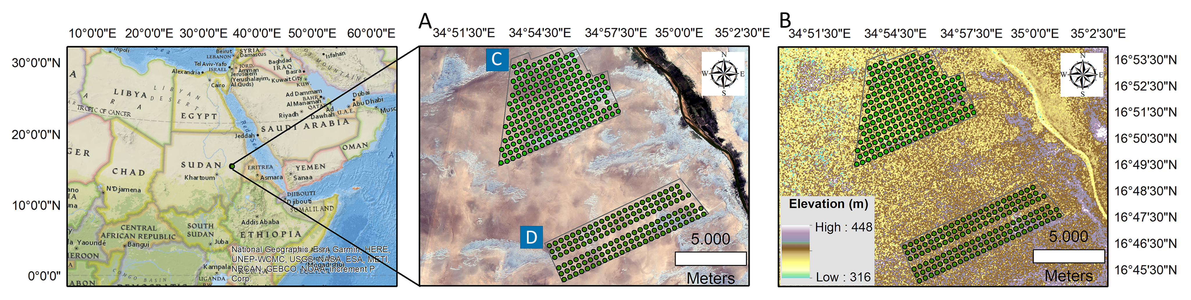
This study was conducted at the lower Atbara Nile, which extends about 270 km SE of Atbara town in River Nile State and nearly 288 km from Khartoum, the capital of Sudan. The study area is located between 16°44′ N and 16°55′ N Latitude and 34°50′ E and 35°2′ E Longitude and covers a total area of about 7600 ha (distributed as 4200 ha for the reference area and 3400 ha for the target area). The study area falls within the desert climatic zone of the country, with an average annual precipitation of 63.2 mm (mainly between July and August), an average annual temperature of 29.6 °C, and an average annual relative humidity of 28.3%. The soil is characterized by hyper-thermic and aridic soil temperature and moisture regimes, respectively. The soil is classified as Aridisols according to soil taxonomy [54,55].
2.2. Field Study and Sampling Strategy
A semi-detailed soil survey was used to perform this study using a scale of 1:45,000. We used a grid design to determine the targeted sample locations. The total auger locations for reference and target areas were 202 and 144 sites, respectively. We used a handheld GPS (Garmin Montana 680t) to determine the precise sites of the auger samples. Figure 1A shows the geographical location of the study area overlaid on the Sentinel 2 MSI natural color band combination map. Figure 1B presents the field distribution of auger samples on the DEM map. Soil samples were taken from a three-depth systematic sampling design [55] at 450 m intervals at both studied areas: 0–30 cm, 30–60 cm, and 60–90 cm, with approximately 0.5 to 1 kg of soil material gathered from each depth. The total number of samples collected was 1041 (608 from the reference area and 432 from the target area).
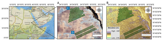
Figure 1.
Spatial distribution of soil sampling points overlaid on Sentinel 2 MSI natural color band combination map (A) and digital elevation model (DEM) (B), including reference area (C) and target area (D). The polygons define the study areas, while the green dots define the soil sampling points.
2.3. Sample Analysis
Soil samples were air dried at ambient room temperature (≈25 °C), ground, and passed through a 2 mm sieve to isolate soil material from rock fragments. Electrical conductivity (ECe) as an indicator of salinity was determined in the extracts of the soil paste [56] using a digital EC meter (Jenway, 4510, UK). According to the FAO salinity classification [34,57] electrical conductivity data (dS m−1) are classified into three classes: None (<2 dS m−1), Moderate (between 2 and 4 dS m−1), and Strong (> 4 dS m−1).
2.4. Environmental Covariates via Google Earth Engine
To estimate salinity variations along the soil depth direction in the study area, relevant environmental covariates were selected due to their influence on salinity levels. Salinity, vegetation, and soil indices based on Sentinel 2 MSI [58], as well as horizontal transmit and vertical receive (HV) and horizontal transmit and horizontal receive (HH) polarization mode backscattering coefficient data from PALSAR-2 [59], along with derived digital elevation model derivatives, were generated using the Google Earth Engine (GEE) data catalog and platform [60]. All digital covariates were extracted from GEE to be aligned on a 10 × 10 m grid and subsequently utilized for mapping purposes.
2.4.1. Synthetic Aperture Radar Data
Since no available images could be obtained in the frames of the Sentinel 1 SAR satellite for the study area, Global PALSAR-2/PALSAR Yearly Mosaic [61,62], version 2 data were transferred from the GEE data catalog to the GEE code editor section [60], taking into account the years closest to the soil sampling dates. The PALSAR/PALSAR-2 mosaic was acquired at 25 m resolution [61]. This dataset is a seamless global SAR image created by mosaicking SAR images from PALSAR/PALSAR-2. In this study, 2018, 2019, and 2020 image collections in HH and HV polarization were then cropped according to the study area scope using the “.filterBounds” script in the GEE code editor [60]. Finally, using the “.mean” script, the mean of their collections was calculated for the study area to reduce data volume and for faster analysis. Polarization data can be obtained as 16 bit digital numbers (DN) and converted to backscatter coefficient values in decibel units (dB) using the following equation [61,63]:
where −83.0 is the calibration factor (dB) for the PALSAR-2 mosaics.
γ0 = 10log10(DN2) − 83
This equation was executed in ArcGIS 10.8—Arctoolbox—Spatial Analyst Tools—Map Algebra—Raster Calculator [64].
2.4.2. Multispectral Satellite Data
Sentinel-2 MSI: MultiSpectral Instrument, Level-2A product was called from the GEE catalog, and 180 images were taken from the catalog by running the “.filter(‘CLOUDY_PIXEL_PERCENTAGE < 5’)” script within 1 year close to the soil sampling date. Using the study area shapefile and the “.filterBounds” script, the satellite image collection was clipped. Again, using the “.mean” script to reduce data volume and for faster analysis, mean synthesis images were calculated for Band 2, Band 3, Band 4, Band 8, Band 11, and Band 12 using all image collections among the respective dates. Salinity, vegetation, and soil indices in Table 1 were generated and used as environmental covariates.
2.4.3. Digital Elevation Model Data
NASADEM Merged DEM Global 1 arc second V001 data [65] was called from the GEE catalog and cut using the “.filterBounds” script according to the study area shapefile. In addition to the elevation data, the slope in degrees was used as an environmental covariate produced by the “ee.Terrain.slope” script.

Table 1.
Environmental covariates are used for predicting soil salinity levels.
Table 1.
Environmental covariates are used for predicting soil salinity levels.
| Remote Sensing (RS) (Sentinel 2) OPTICAL-Based Covariates | Equations [27,32,35,58,66] |
|---|---|
| Band 2 | Blue (Central Wavelength: 490 nm) |
| Band 3 | Green (Central Wavelength: 560 nm) |
| Band 4 | Red (Central Wavelength: 665 nm) |
| Band 8 | NIR (Central Wavelength: 842 nm) |
| Band 11 | SWIR1 (Central Wavelength: 1610 nm) |
| Band 12 | SWIR1 (Central Wavelength: 2190 nm) |
| Normalized Difference Vegetation Index (NDVI) | |
| Carbonate Normalized Ratio (CNR) | |
| Clay Normalized Ratio (CLNR) | |
| Ferrous Normalized Ratio (FNR) | |
| Iron Normalized Ratio (INR) | |
| Normalized Difference Moisture Index (NDMI) | |
| Rock Outcrop Normalized Ratio (RONR) | |
| Green-Red vegetation index (GRVI) | |
| Saturation index (SatInd) | |
| Green Normalized Difference Vegetation Index (GNDVI) | |
| Salinity Index 1 | |
| Salinity Index 2 | |
| Salinity Index 3 | |
| Salinity Index 4 | |
| Salinity Index 5 | |
| Salinity Index 6 | |
| Remote Sensing (RS) (PALSAR/PALSAR-2 mosaic) synthetic aperture RADAR-based covariates [59,61] | |
| AVG_HH_dB-polarization backscattering coefficient | For horizontal transmit and horizontal receive |
| AVG_HV_dB-polarization backscattering coefficient | For horizontal transmit and vertical receive |
| DEM-based primary covariates at NASA JPL [65] | |
| Elevation | m unit |
| Slope | Degree unit |
NIR: Near infrared, SWIR: Shortwave infrared.
2.5. Modelling Salinity Levels and Transferability of Models
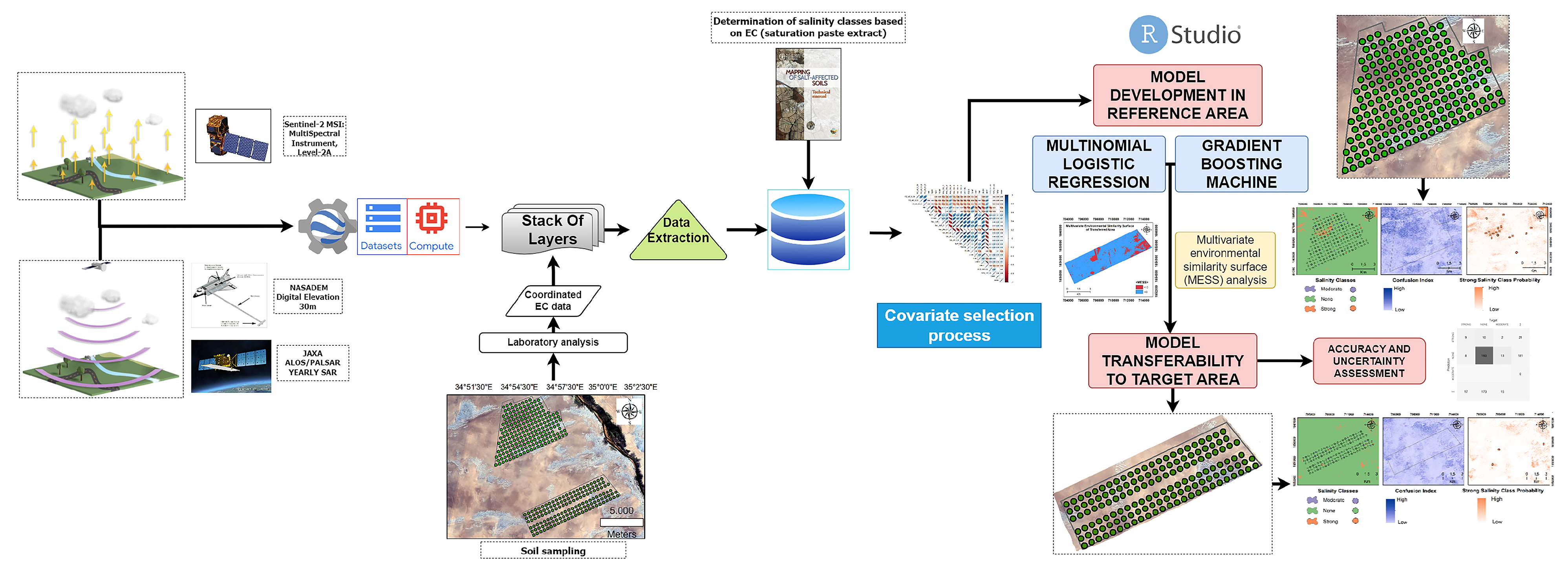
This study followed the DSM framework and involved several steps in the modeling process: (1) enabling and curating soil data; (2) obtaining environmental covariates from open sources; (3) extracting georeferenced sample points from the digital covariate data and preparing geodatabases [67]; (4) selecting environmental covariates through the use of “findCorrelation” functions to identify and eliminate highly correlated covariates; (5) performing classification-based modeling of salinity levels; and (6) transferring the models. The flowchart of the study is depicted in Figure 2.
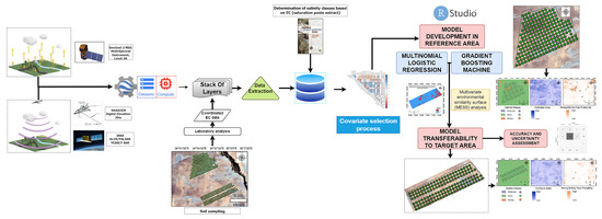
Figure 2.
Flowchart of the methodology.
The “findCorrelation” function in the “caret” package [68] was run to identify highly correlated covariates that could also compromise the performance of the model. Covariates with Spearman correlation coefficients above 0.8 were removed (Figure A1) [69,70].
To build a statistical model between environmental covariates and the predicted soil salinity classes, 2 different mathematically-based ML algorithms were systematically compared: Multinomial Logistic Regression [71,72] and Gradient Boosting Machine [73,74].
In the study, soil salinity classes are the outcome variables. In the process of data import in R core environment software [75], the categories of salinity classes were coded alphabetically as 1 (None), 2 (Moderate), and 3 (Strong). Specifically, two logit functions are needed in the three-outcome category model. The modeler can decide which outcome category to use as the reference, for which the class “1 (None)” was chosen in numerical order. Logit functions comparing the other 2 classes with the reference were created. All these processes were carried out with the “multinom” function in the “caret” package [68]. Due to the nature of the multinomial logistic regression algorithm, a pixel can belong to all three different soil salinity classes with given probabilities [76]. However, the salinity class with the highest probability is assigned to the pixel.
The Gradient Boosting Machine (GBM) is one of the most powerful MLAs for classification problems [77] involved in our study. Like tree-based learners in RF, GBM is an ensemble method based on decision trees [78]. However, unlike RF, this method generates trees serially, with each tree attempting to improve the prediction by correcting the errors of the previous one.
The hyperparameters of each ML algorithm were set using their respective packages “nnet” [72] and “gbm” [74] (Table 2). Using R Core Environment software (Version 4.2.1) [75] and RStudio IDE [79], soil salinity classes at 3 different depths in the reference study area and CLNR, FNR, NDVI, AVG_HH_dB, AVG_HV_dB, Elevation, Slope, and Salinity Index 1 were selected and estimated using these environmental covariates.
Table 2.
Parameters for the machine learning algorithms used and final environmental covariates included for predicting soil salinity levels.
Descriptive statistical parameters were computed for the values of the eight chosen digital covariates within both the reference and target regions. Furthermore, Multivariate Environmental Similarity Surfaces were calculated [80] to compare the compatibility of the values of environmental variables in the dataset in the reference area with those in the target area to be transferred. This method can be used to measure the similarity between the selected covariates at the location of the training samples and the target area to be transferred [81,82]. Values lower than zero indicate prediction locations in both feature and geographic areas that are not explained by the training samples [82]. The MESS map for the target region was generated using the “mess” function in the “dismo” package [80].
2.6. Importance of Used Covariates in Models, Accuracy, and Uncertainty Evaluations
The relative importance levels of different digital environmental variables in the prediction models of salinity classes were calculated using the “varImp” function in the caret package [68].
In digital soil mapping, user accuracy (UA) and producer accuracy (PA) are used to validate the performance of different algorithms in both reference and target areas [66]. The “cvms” R package [83] was used to estimate the performance measures of the classification models through the confusion matrix, while the Tau index, whose performance on unbalanced datasets is emphasized by Rossiter et al. [84], was calculated using the “tauW” function in the “aqp” package [85]. When the value of the Tau index approaches 1, it indicates a strong indication of perfect agreement. In the study, both algorithms calculate probability values for each salinity class on a pixel basis, and for uncertainty evaluation, the confusion index (CI) is calculated, which spatially measures the confusion between the most probable salinity class and the second most probable class [86,87].
3. Results
Section 3.1 provides descriptive statistics on continuous and categorical soil salinity data. While Section 3.2 presents the performance measures of two different algorithms, Section 3.3 contains findings on the transfer of models to the target area. Section 3.4 includes maps of soil salinity classes and confusion index maps produced by two different algorithms at three depths. Section 3.5 contains information about the importance of environmental variables used in models.
3.1. Results of Measured Electrical Conductivity and Assessment of Salinity Classes
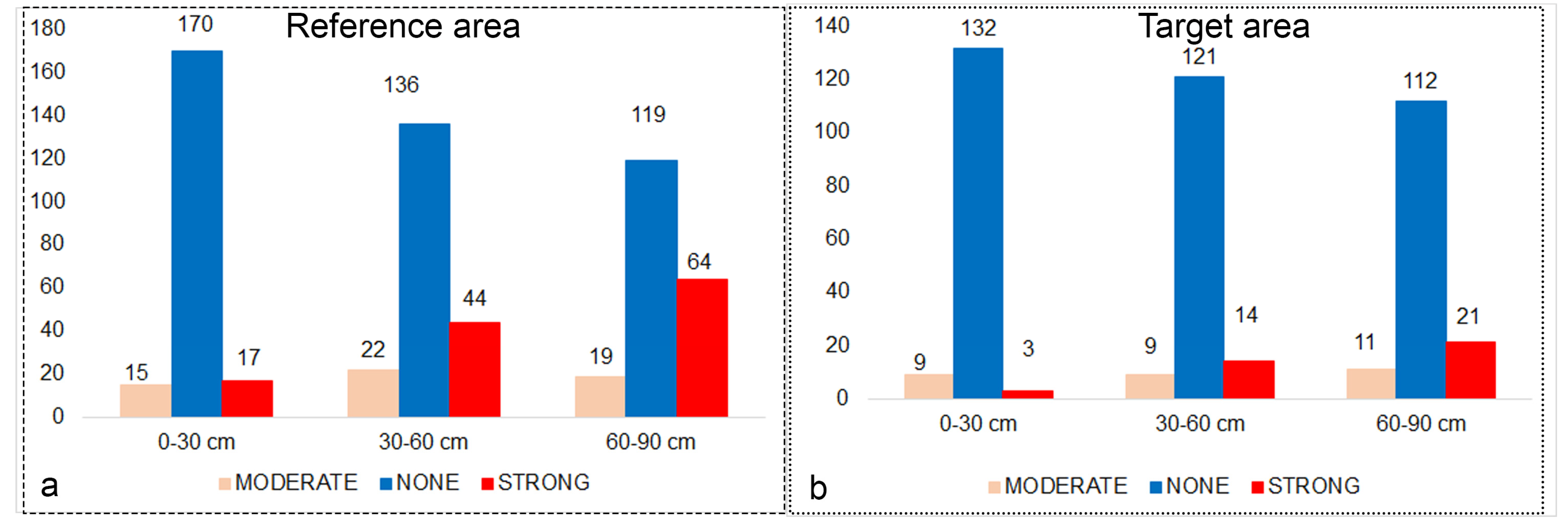
Descriptive statistics and histograms of the reference area and target area sample sets taken from three different depths are shown in Figure A2. The distribution of reference area and target area samples according to salinity classes was relatively unbalanced (Figure 3a,b). Both in the reference region and in the target region, the number of observations of the “strong” salinity class increased with depth, while the “None” salinity class decreased (Figure 3a,b).
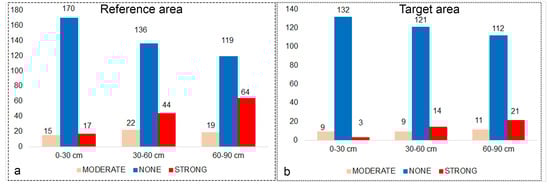
Figure 3.
Distribution of observations by salinity classes in the reference (a) and target (b) area. The y axis is the number of samples.
3.2. Performance of the Different Classification Algorithms
The validation statistics of soil salinity classes for each algorithm are presented in Table 3. The results of the confusion matrix from which the table was generated are presented in Figure A3. The highest Tau index values were obtained for both the reference area and the target area in the 0–30 cm samples, which can be considered surface samples (Table 3). The decrease in Tau index values followed a linear trend as the depth increased (Table 3). MNLR and GBM algorithms indeed provided very close performance measures when Tau index values were considered (Table 3).
Table 3.
Summary of machine learning algorithms performance criteria for reference area and transferred area.
In the surface samples (0–30 cm), the user’s accuracy values for the “none” class were above 90% for the target area (Table 3). However, in both models, the remaining two classes failed to be predicted. After a careful examination of the confusion matrix (Figure A3), the models assigned the “strong” and “moderate” classes to the “none” classes.
Considering the distribution of the number of classes at different depths (Figure 3), this may be due to the fact that these models do not have enough observations to learn the classes. As a matter of fact, the user’s accuracy values for the “strong” class could compute an increase in depth (30–60 cm and 60–90 cm). As the depth increased, the number of observations of the “strong” class also increased.
3.3. Transferability of Models according to Multivariate Environmental Similarity Surface
Since eight environmental variables were used in the modeling process, the selected variables in Table 2 were used for similarity analysis during the transfer of the models. Descriptive statistics of selected radar, optic-based, and terrain covariates at the sampling locations in the reference and target areas are shown in Table 4. The minimum values of the radar-based covariates are quite close for both areas (Table 4). A similar situation was found in the optical-based FNR, NDVI, and CLNR covariates (Table 4). In particular, the distributions of the land covariates are also basically similar across the regions, and the standard deviation values are quite close to each other (Table 4).
Table 4.
Descriptive statistics for environmental variables for both reference and target areas.
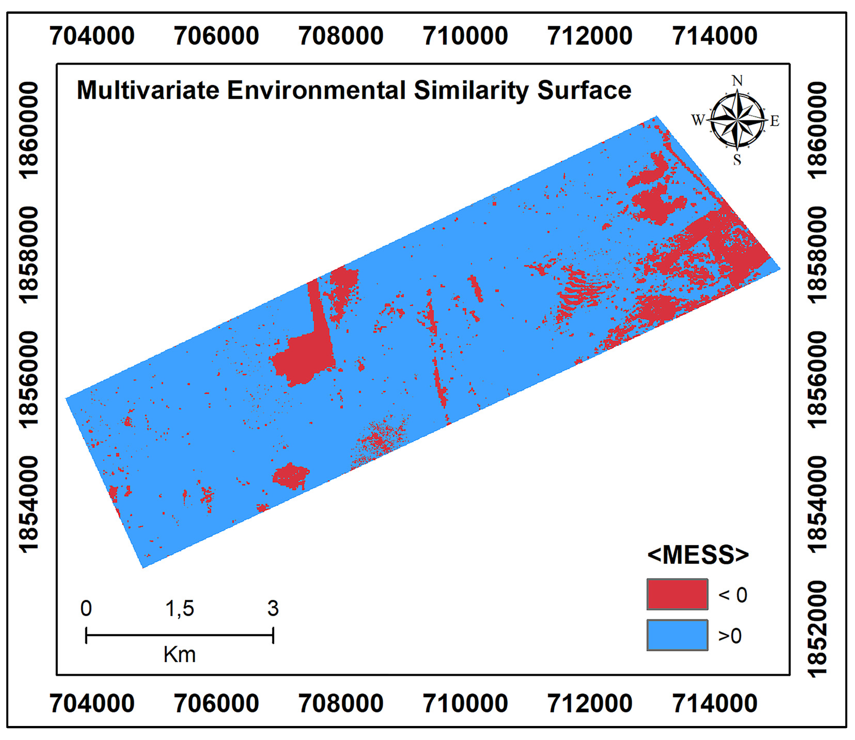
According to the environmental variable values of the observations in the reference area and the MESS results of the target region (Figure 4), the models can be effectively transferred for regions with values above 0. However, MESS values below 0 in the southeast of the target area are associated with the accumulation of wind-borne materials. Again, the partial excavation of the surface soil in the central part of the study area proves that this area does not have similar environmental variable values (smaller than 0) to the reference region.

Figure 4.
Multivariate Environmental Similarity Surfaces (MESS) for the target area, calculated with the selected covariates according to the reference area.
3.4. Spatial Prediction of Soil Salinity Levels in Reference and Target Areas
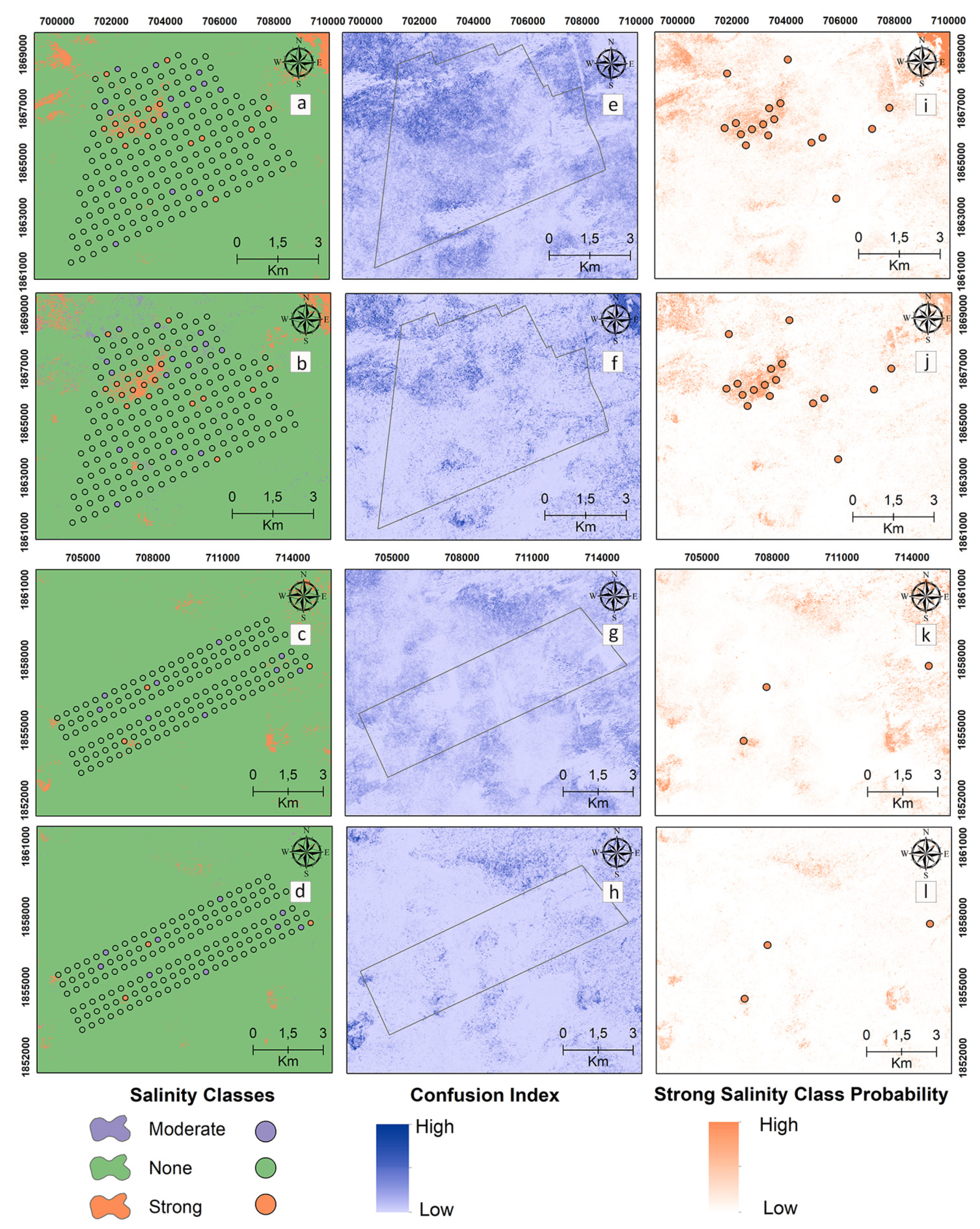
Digital maps of the salinity classes of the 0–30 cm samples are presented in Figure 5 for the reference and target areas by applying MNLR and GBM. The “strong” class was mapped with high probability by the models in the reference area (Figure 5i,j). In the surface samples, MNLR and GBM models produced maps with similar salinity class patterns for both reference and target areas (Figure 5i,j).
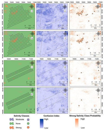
Figure 5.
Digital maps of salinity classes (0–30 cm). Generated by applying the MNLR (a) and GBM (b) models for the reference area as well as the MNLR (c) and GBM (d) models for the target area. For the reference area, confusion index maps for MNLR (e) and GBM (f) as well as MNLR (g) and GBM (h) for the target area. Probability map of the “Strong” salinity class in the reference area obtained by applying the MNLR model (i) and the GBM model (j) as well as the MNLR model (k) and the GBM model (l) for the target area.
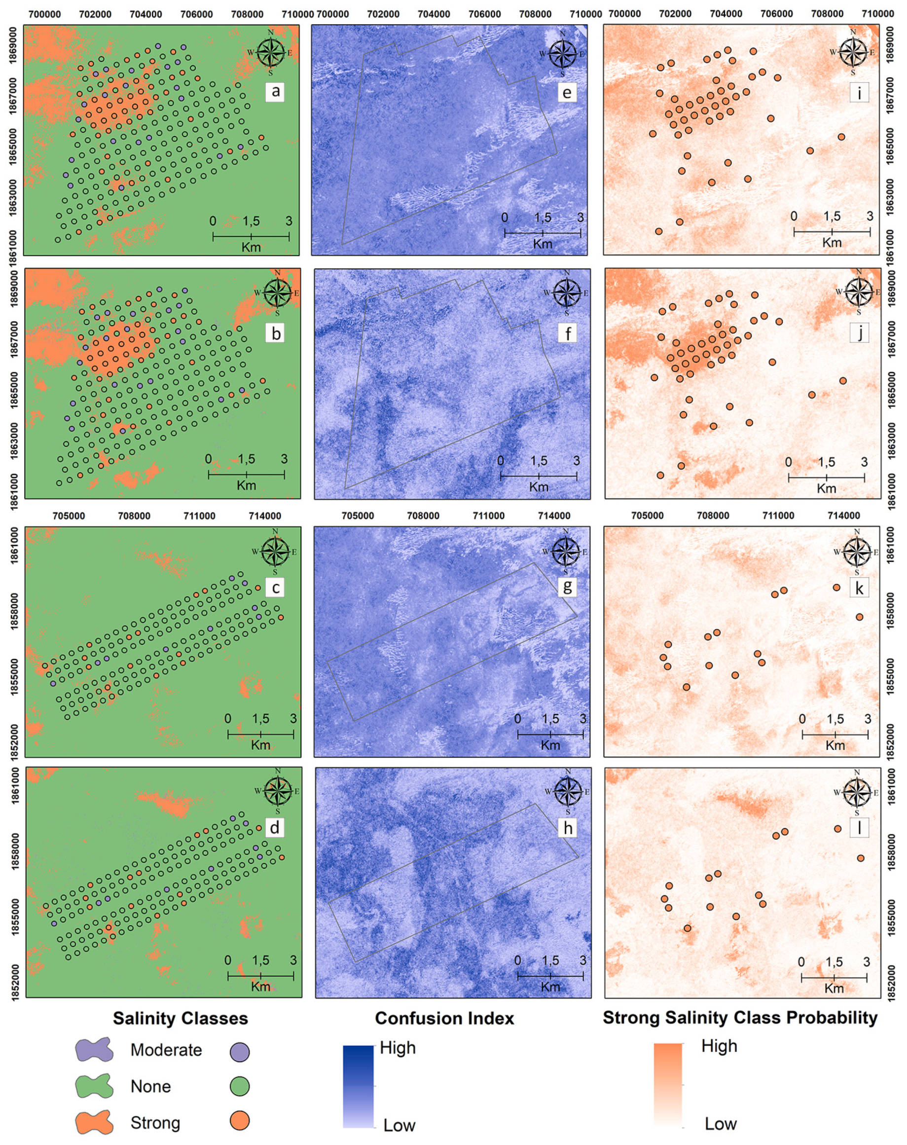
Digital maps of the salinity classes of the 30–60 cm samples are presented in Figure 6 for the reference and target areas by applying MNLR and GBM. Unlike the 0–30 cm maps, the presence of the “strong” salinity class increased in the northwest of the reference area (Figure 6a,b). The “strong” class was mapped with a higher probability by the GBM model in the reference area (Figure 6j). In the 30–60 cm samples, the MNLR and GBM models do not seem to be effective in spatially predicting the “strong” salinity class for the target area. The CI values, which show the difference between the probability values of the most probable and 2nd most probable classes, are higher at 30–60 cm compared to the surface samples (0–30 cm) (Figure 6e–h).
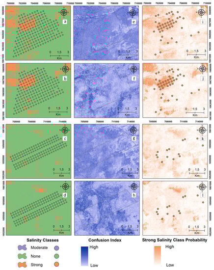
Figure 6.
Digital maps of salinity classes (30–60 cm). Generated by applying the MNLR (a) and GBM (b) models for the reference area as well as the MNLR (c) and GBM (d) models for the target area. For the reference area, confusion index maps for MNLR (e) and GBM (f) as well as MNLR (g) and GBM (h) for the target area. Probability map of the “Strong” salinity class in the reference area obtained by applying the MNLR model (i) and the GBM model (j) as well as the MNLR model (k) and the GBM model (l) for the target area.
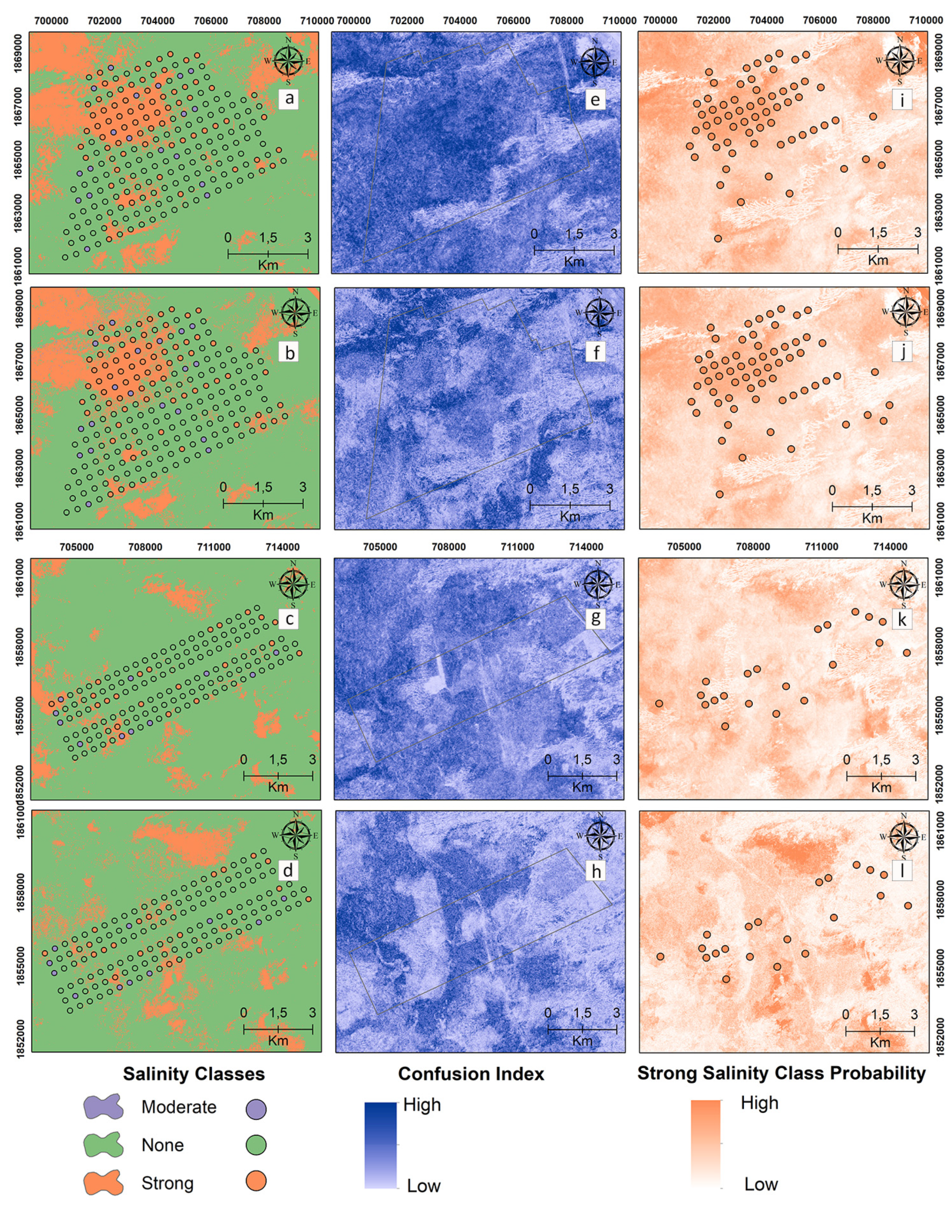
Digital maps of the salinity classes of the 60–90 cm samples are presented in Figure 7 for the reference and target areas by applying MNLR and GBM. Unlike the previous two depth maps, the presence of the “strong” salinity class increased northwest of the reference area at 60–90 cm, where the deepest sampling occurred (Figure 7a,b). In the 60–90 cm samples, the MNLR and GBM models were not effective in spatially predicting the “strong” salinity class for the target area. The CI values, which show the difference between the probability values of the most probable and 2nd most probable classes, are higher at 60–90 cm compared to the two depth maps (Figure 7e–h).
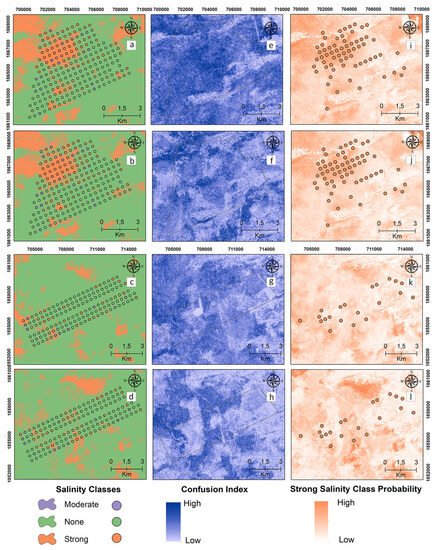
Figure 7.
Digital maps of salinity classes (60–90 cm). Generated by applying the MNLR (a) and GBM (b) models for the reference area as well as the MNLR (c) and GBM (d) models for the target area. For the reference area, confusion index maps for MNLR (e) and GBM (f) as well as MNLR (g) and GBM (h) for the target area. Probability map of the “Strong” salinity class in the reference area obtained by applying the MNLR model (i) and the GBM model (j) as well as the MNLR model (k) and the GBM model (l) for the target area.
Considering the three different depths of soil salinity classes in the digital maps (Figure 5, Figure 6 and Figure 7), the presence of a “strong” class increases with depth in the northwest of the reference area, both in the samples taken and in the predicted maps. The current salinity risk in the northwest region of the reference area was found to be high, and high-resolution (10 m) digital maps can play an effective role in defining the management zones for salinity.
3.5. Importance of Environmental Variables
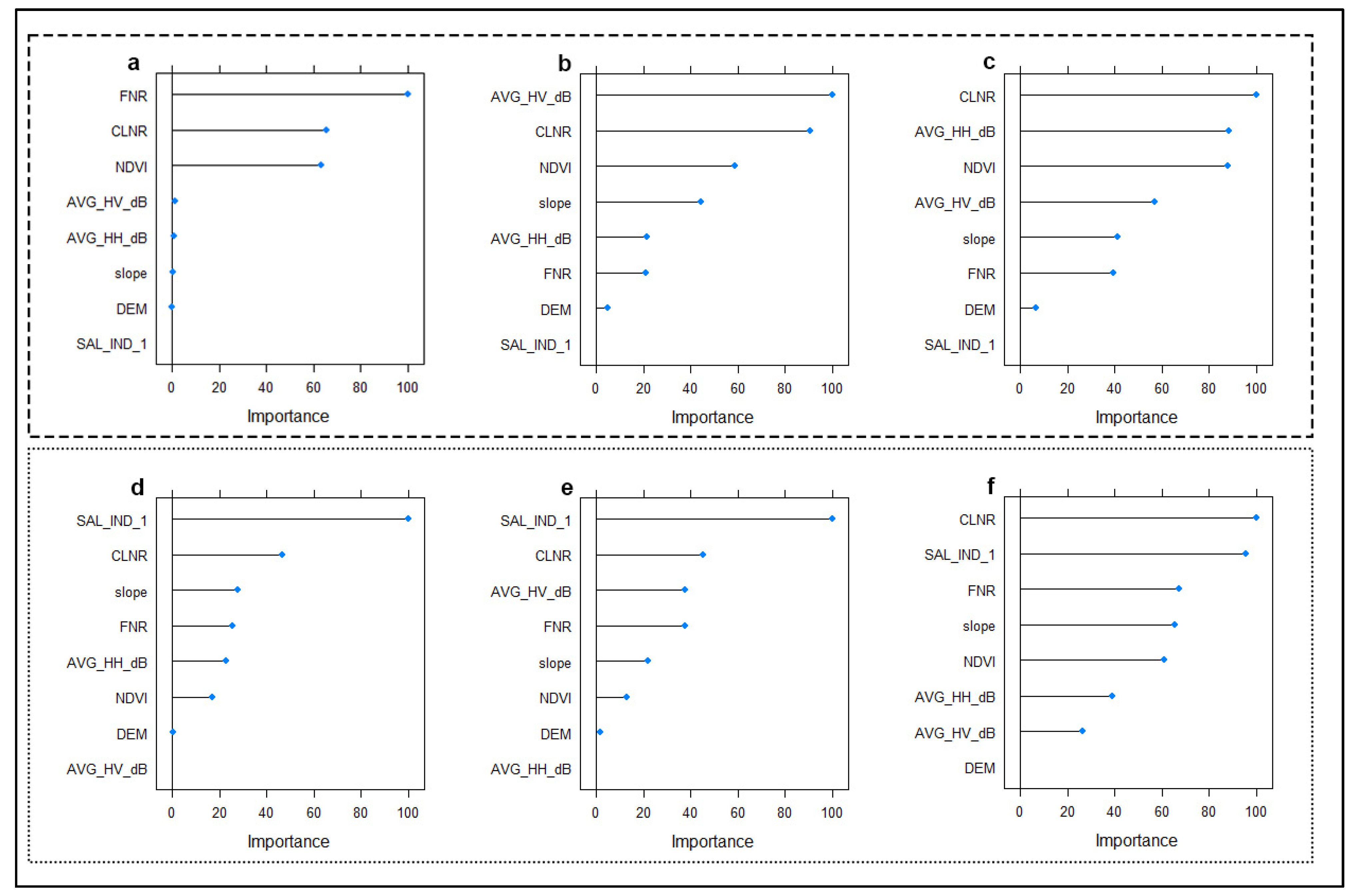
Figure 8 shows the relative importance of the environmental variables used in modeling soil salinity classes at the three different depths. In both models, the salinity class of surface soils is determined by the indices produced from optical-based satellite images (Figure 8a,d). In the MNLR model, the relative importance of SAR data increased in the modeling of 30–60 and 60–90 samples (Figure 8b,c). In the GBM model, the increase is not as noticeable as in MNLR (Figure 8e,f). In arid areas, salinity and soil-based indices seem to be relatively more important for the models than vegetation indices.
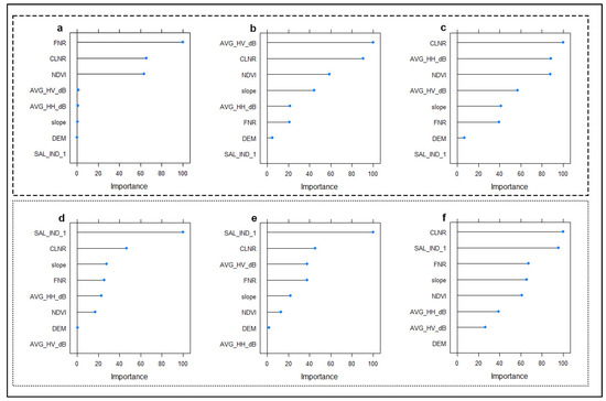
Figure 8.
Importance of environmental variables in predicting soil salinity classes using different algorithms. 0–30 cm (a), 30–60 cm (b), and 60–90 cm (c) for MNLR (Multinomial Logistic Regression). 0–30 cm (d), 30–60 cm (e), and 60–90 cm (f) for GBM (Gradient Boosting Machine).
4. Discussion
The most accurate spatial determination and subsequent monitoring of soil salinity are crucial for sustainable agriculture and food security [3,6]. Up-to-date, reliable, and accurate assessments of soil salinity are important for land use planners and managers. In our study, a three-class estimation process was carried out, and Tau index values were found to be very similar to the Tau value of 0.74 reported by Omuto et al. [57] in Northwestern Sudan. Differences in the relative overall accuracy or Tau index values in the literature comparisons of classification results may be due to the number of salinity classes. For example, Kumar et al. [88] mapped the salt-affected areas with the logistic regression model in their study in the part of the Indo–Gangetic plain affected by soil salinity, with an overall accuracy of 81%.
Since soil salinity is a dynamic environmental problem, it is critical to monitor temporal and spatial changes [57]. Considering the temporal variability of soil salinity, the use of advanced sensor technologies for precision agriculture applications in the future [89], both in the study area and in similar regions, can be used to optimize the growing conditions [90]. Especially in arid regions where irrigated agriculture is practiced, Zhu et al. [91] emphasized the importance of creating soil salinity maps in terms of changes in soil salinity during the irrigated or non-irrigated period to understand the main mechanisms causing soil salinity.
Two ML algorithms that make predictions based on relatively different mathematical calculations presented the results of a comparative study in an arid region of Sudan to assess the transferability of salinity classes using selected covariates. The majority of misclassified and unpredicted cases were found within the moderate salinity class in both the reference and target areas. However, the primary objective of this study is not centered around maximizing the predictive accuracy of the models; rather, it aims to provide initial insights into the transferability of soil salinity models with relevance to agronomic applications. Although the reference and target areas are characterized by very similar climates and topographies [92], there may be concerns about quantifying the degree of similarity between them based on more quantitative results just before model transfer. Therefore, it is recommended for future studies to present comparative results of different mathematical bases such as the Gower similarity index [93] and dissimilarity index [94]. Enhancing the predictive accuracy of transferability related to soil salinity can involve the exploration of specific geographical stratifications [53], such as physiography or topography (slope-aspect categories), as well as the consideration of land use factors.
The low variation in elevation and the homogeneity of the climate in the study area may have caused the elevation digital covariate to be ineffective in the modeling. The effectiveness of optical satellite-based salinity indices [27,32,35,95] and SAR data are consistent with the literature [5,29]. Nevertheless, our effort has been to leverage remote sensing data for the purpose of transferring salinity class models to research areas characterized by quantified similarity analysis. The study outcomes have revealed the substantial transferability of satellite-based radar and optical environmental variables within an arid region, substantiating their potential for generating beneficial outputs. For transferability of soil salinity levels in arid regions using ML algorithms, the PlanetScope satellite [96] can offer important opportunities to capture the spatial variability of salinity [97].
The ultimate aim is to produce useful insights as a result of the models. Among the salinity class maps resulting from the study, special attention should be paid to the spatial distribution of the “strong” class. Our study includes not only defining the problem but also searching for solutions. In this regard, Soil-Improving Cropping Systems, which aim to prevent, mitigate, or ameliorate the adverse effects of soil salinity and improve associated soil functions and ecosystem services related to agricultural production, should be given importance [98]. Sugarcane, which is an important crop in Sudan [44,99], is a very sensitive plant to salinity in terms of cultivation [8,100]. In this study, the cultivation of this deep-rooted plant in areas with increasing “strong” class probability and especially in areas where the danger of salinity increases with depth may experience negative effects. It is important to select plants with relatively high resistance in saline environments [101,102]. As a matter of fact, the study area right next to the Atbara River should be subjected to evaluations such as irrigated land classification [103,104] in a wider perspective for its effective use in irrigated agriculture activities.
Future work should center on assessing the temporal and spatial transferability of remote sensing, including its capability to detect fluctuations within soil salinity classes. While the determination of large-scale soil limitations with DSM methodology is an important objective, ML models are increasingly being used for this purpose. However, it is well known that tree-based algorithms are sensitive to extrapolation, i.e., transferability [105]. In tree-based learners (GBM in our study), any split threshold within the nodes for the “y” (dependent) variable is limited by the minimum and maximum value range of the particular feature in the training dataset [105]. Therefore, when the algorithm encounters a value of “y” that is outside the bounds of the training dataset, it applies the closest corresponding dependent variable value from the training dataset in the mathematical prediction process. Therefore, it will be more difficult to extrapolate regression-based estimates of transferability for tree-based learners. Soil scientists skilled in the mathematics of the models are important at the point of applicability of ML to soil data [106]. It enables more applicable methodologies for transferability by harmonizing the EC values into salinity classes (categorical data) that adhere to international standards for continuous data types.
Furthermore, future studies should focus on measuring the transferability risk associated with MLAs for soil salinity prediction while also focusing on research that will help assess the reliability of their predictions [107]. These studies can reveal valuable information regarding the integration of ML model predictions into the decision/support system [108]. It can be recommended in research for predictive models to provide information at the reconnaissance scale [109].
5. Conclusions
In this study, we integrated indices generated from long-term optical Sentinel data and PALSAR-2 radar imagery through GEE for digital mapping of high-resolution regional-scale soil salinity classes in Sudan. We also addressed the transferability of ML-based soil salinity classes in arid areas and used MESS before transferring from the reference area to the target area. This paper presents transfer learning techniques for fast and accurate soil salinity mapping using open-access digital data and machine learning algorithms. In this process, soil scientists should be well-skilled in the mathematical basis of algorithms for integrating soil data to be transferred by modeling into the ML. The spatial information on soil salinity generated in this study can provide remarkable insights into decision-making processes that are compatible with the growing need for soil information for future sustainable development goals.
Author Contributions
Conceptualization, F.K. and M.M.S.; methodology, F.K. and M.M.S.; software, F.K.; formal analysis, F.K.; investigation, M.M.S. and M.A.E.; resources, M.M.S. and M.A.E.; data curation, F.K. and M.M.S.; writing—original draft preparation, F.K. and M.M.S.; writing—review and editing, M.M.S., F.K., M.A.E., L.B. and R.F.; visualization, F.K. All authors have read and agreed to the published version of the manuscript.
Funding
This research received no external funding.
Data Availability Statement
The data presented in this study are available on request from the first author.
Conflicts of Interest
The authors declare no conflict of interest.
Appendix A
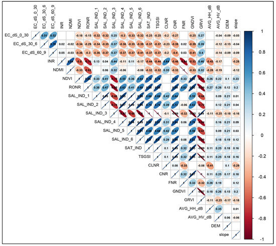
Figure A1.
Spearman correlation analysis of environmental variables. Blue color indicates a positive correlation, while red color exhibits a negative correlation at p < 0.05. Empty boxes indicate no correlation between parameters.
Figure A1.
Spearman correlation analysis of environmental variables. Blue color indicates a positive correlation, while red color exhibits a negative correlation at p < 0.05. Empty boxes indicate no correlation between parameters.
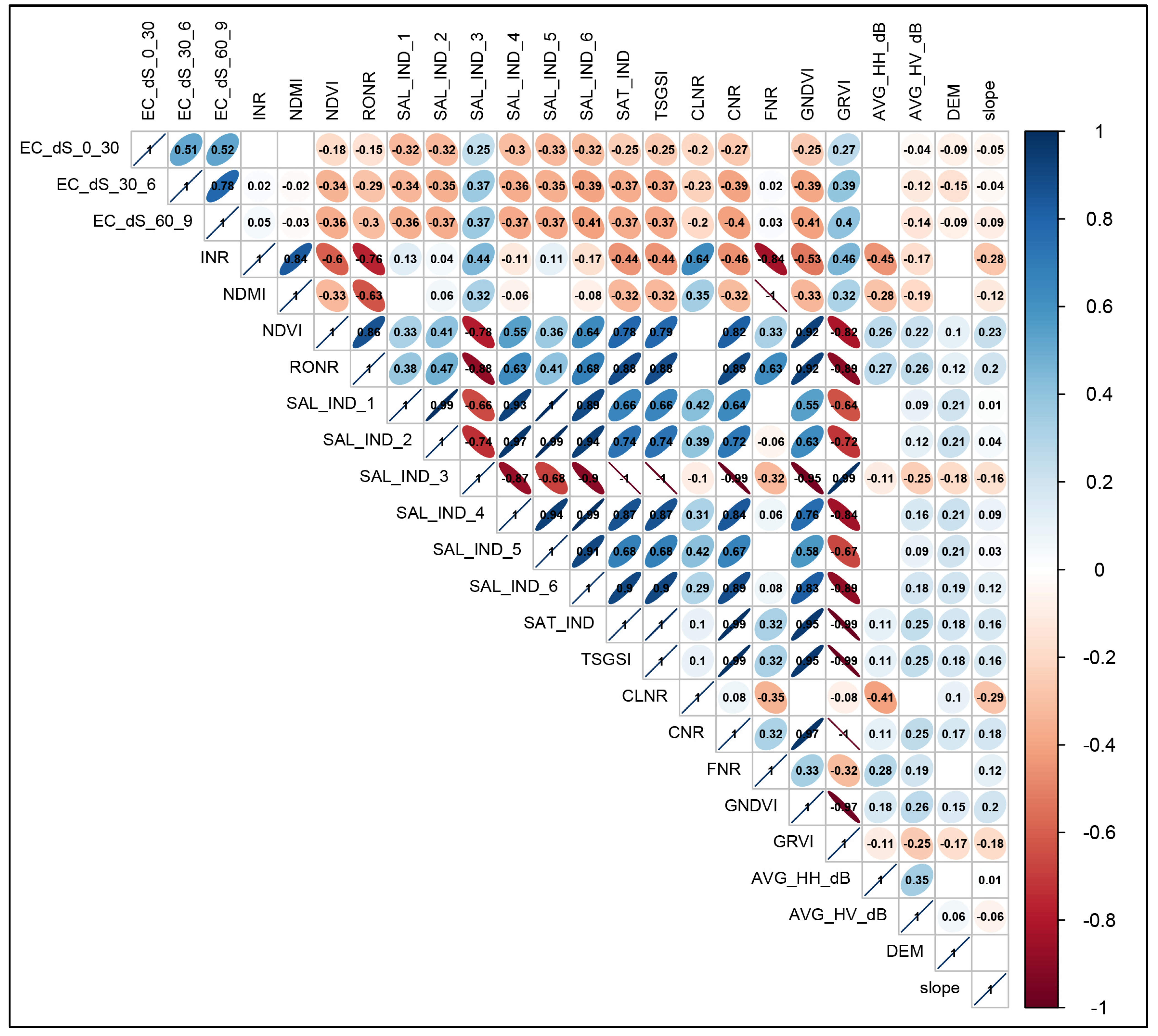
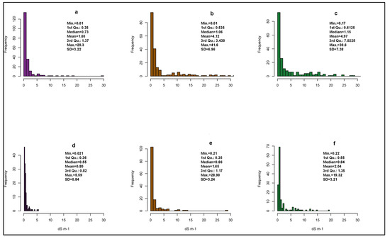
Figure A2.
Histograms of measured EC at reference and target sites and some descriptive statistics. 0–30 cm (a), 30–60 cm (b), and 60–90 cm (c) for the reference area. 0–30 cm (d), 30–60 cm (e), and 60–90 cm (f) for the target area.
Figure A2.
Histograms of measured EC at reference and target sites and some descriptive statistics. 0–30 cm (a), 30–60 cm (b), and 60–90 cm (c) for the reference area. 0–30 cm (d), 30–60 cm (e), and 60–90 cm (f) for the target area.
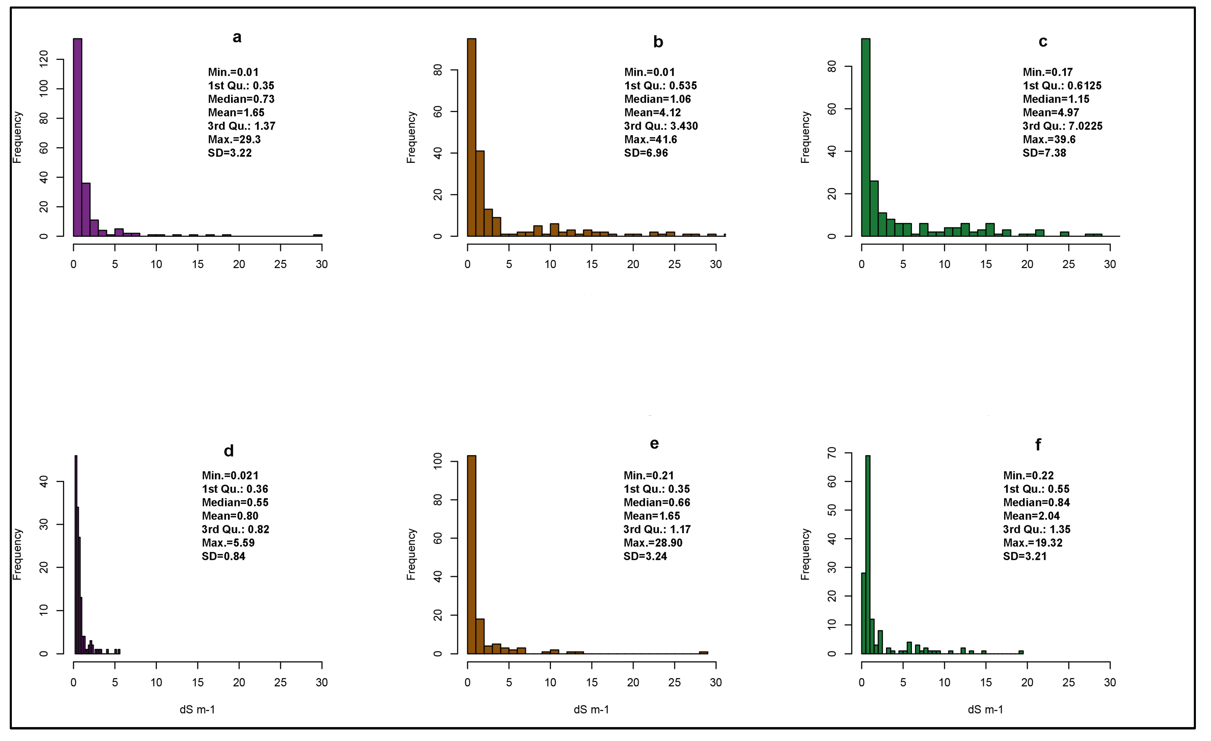
Figure A3.
Confusion matrix results of the classification performances of the models for reference and target areas. Confusion matrices of 0–30 cm (a), 30–60 cm (b), 60–90 cm (c) maps produced by applying the MNLR model for reference area and 0–30 cm (d), 30–60 cm (e), 60–90 cm (f) maps produced by applying the GBM model. Confusion matrices of 0–30 cm (g), 30–60 cm (h), 60–90 cm (i) maps produced by applying the MNLR model and 0–30 cm (j), 30–60 cm (k), 60–90 cm (l) maps produced by applying the GBM model for the target area.

References
- FAO. GSASmap v1.0, Global Map of Salt-Affected Soils. Available online: https://www.fao.org/3/cb7247en/cb7247en.pdf (accessed on 7 September 2022).
- Kaya, F.; Schillaci, C.; Keshavarzi, A.; Basayigit, L. Predictive Mapping of Electrical Conductivity and Assessment of Soil Salinity in a Western Türkiye Alluvial Plain. Land 2022, 11, 2148. [Google Scholar] [CrossRef]
- Negacz, K.; Vellinga, P.; Barrett-Lennard, E.; Choukr-Allah, R.; Elzenga, T. (Eds.) Future of Sustainable Agriculture in Saline Environments; CRC Press: Boca Raton, FL, USA, 2021. [Google Scholar]
- Hazbavi, Z.; Zabihi Silabi, M. Innovations of the 21st Century in the Management of Iranian Salt-Affected Lands. In Future of Sustainable Agriculture in Saline Environments; Negacz, K., Vellinga, P., Barrett-Lennard, E., Choukr-Allah, R., Elzenga, T., Eds.; CRC Press: Boca Raton, FL, USA, 2021; pp. 147–170. [Google Scholar]
- Zdruli, P.; Zucca, C. Restoring Land and Soil Health to Ensure Sustainable and Resilient Agriculture in the Near East and North Africa Region—State of Land and Water Resources for Food and Agriculture Thematic Paper; Zdruli, P., Zucca, C., Eds.; FAO: Cairo, Egypt, 2023. [Google Scholar]
- Negacz, K.; Malek, Ž.; de Vos, A.; Vellinga, P. Saline Soils Worldwide: Identifying the Most Promising Areas for Saline Agriculture. J. Arid Environ. 2022, 203, 104775. [Google Scholar] [CrossRef]
- Mukhopadhyay, R.; Sarkar, B.; Jat, H.S.; Sharma, P.C.; Bolan, N.S. Soil Salinity under Climate Change: Challenges for Sustainable Agriculture and Food Security. J. Environ. Manag. 2021, 280, 111736. [Google Scholar] [CrossRef] [PubMed]
- Singh, A. Soil Salinity: A Global Threat to Sustainable Development. Soil Use Manag. 2022, 38, 39–67. [Google Scholar] [CrossRef]
- Singh, A. Soil Salinization Management for Sustainable Development: A Review. J. Environ. Manag. 2021, 277, 111383. [Google Scholar] [CrossRef]
- Basak, N.; Rai, A.K.; Barman, A.; Mandal, S.; Sundha, P.; Bedwal, S.; Kumar, S.; Yadav, R.K.; Sharma, P.C. Salt Affected Soils: Global Perspectives. In Soil Health and Environmental Sustainability; Shit, P.K., Adhikary, P.P., Bhunia, G.S., Sengupta, D., Eds.; Springer Science and Business Media Deutschland GmbH: Berlin/Heidelberg, Germany, 2022; pp. 107–129. [Google Scholar]
- Devkota, K.P.; Devkota, M.; Rezaei, M.; Oosterbaan, R. Managing Salinity for Sustainable Agricultural Production in Salt-Affected Soils of Irrigated Drylands. Agric. Syst. 2022, 198, 103390. [Google Scholar] [CrossRef]
- Cf, O.D.D.S. United Nations General Assembly Transforming Our World: The 2030 Agenda for Sustainable Development; United Nations: New York, NY, USA, 2015. [Google Scholar]
- Tomaz, A.; Palma, P.; Alvarenga, P.; Gonçalves, M.C. Soil Salinity Risk in a Climate Change Scenario and Its Effect on Crop Yield. In Climate Change and Soil Interactions; Elsevier: Amsterdam, The Netherlands, 2020; pp. 351–396. [Google Scholar] [CrossRef]
- Okur, B.; Örçen, N. Soil Salinization and Climate Change. In Climate Change and Soil Interactions; Elsevier: Amsterdam, The Netherlands, 2020; pp. 331–350. [Google Scholar] [CrossRef]
- Keshavarzi, A.; del Árbol, M.Á.S.; Kaya, F.; Gyasi-Agyei, Y.; Rodrigo-Comino, J. Digital Mapping of Soil Texture Classes for Efficient Land Management in the Piedmont Plain of Iran. Soil Use Manag. 2022, 38, 1705–1735. [Google Scholar] [CrossRef]
- Tziolas, N.; Tsakiridis, N.; Ogen, Y.; Kalopesa, E.; Ben-Dor, E.; Theocharis, J.; Zalidis, G. An Integrated Methodology Using Open Soil Spectral Libraries and Earth Observation Data for Soil Organic Carbon Estimations in Support of Soil-Related SDGs. Remote Sens. Environ. 2020, 244, 111793. [Google Scholar] [CrossRef]
- Wang, J.; Zhen, J.; Hu, W.; Chen, S.; Lizaga, I.; Zeraatpisheh, M.; Yang, X. Remote Sensing of Soil Degradation: Progress and Perspective. Int. Soil Water Conserv. Res. 2023, 11, 429–454. [Google Scholar] [CrossRef]
- Bennett, J.M.L.; Roberton, S.D.; Ghahramani, A.; McKenzie, D.C. Operationalising Soil Security by Making Soil Data Useful: Digital Soil Mapping, Assessment and Return-on-Investment. Soil Secur. 2021, 4, 100010. [Google Scholar] [CrossRef]
- Malone, B.; Arrouays, D.; Poggio, L.; Minasny, B.; McBratney, A. Digital Soil Mapping: Evolution, Current State and Future Directions of the Science. Ref. Modul. Earth Syst. Environ. Sci. 2022, 4, 684–695. [Google Scholar] [CrossRef]
- Miller, B.A. Digital Soil Mapping and Pedometrics. In International Encyclopedia of Geography: People, the Earth, Environment and Technology; John Wiley & Sons, Ltd.: Oxford, UK, 2017; pp. 1–8. [Google Scholar]
- European Commission. Soil Monitoring and Resilience (Soil Monitoring Law); European Commission: Brussels, Belgium, 2023. [Google Scholar]
- Rezaei, M.; Mousavi, S.R.; Rahmani, A.; Zeraatpisheh, M.; Rahmati, M.; Pakparvar, M.; Jahandideh Mahjenabadi, V.A.; Seuntjens, P.; Cornelis, W. Incorporating Machine Learning Models and Remote Sensing to Assess the Spatial Distribution of Saturated Hydraulic Conductivity in a Light-Textured Soil. Comput. Electron. Agric. 2023, 209, 107821. [Google Scholar] [CrossRef]
- Mousavi, S.R.; Sarmadian, F.; Omid, M.; Bogaert, P. Three-Dimensional Mapping of Soil Organic Carbon Using Soil and Environmental Covariates in an Arid and Semi-Arid Region of Iran. Measurement 2022, 201, 111706. [Google Scholar] [CrossRef]
- Sahbeni, G.; Ngabire, M.; Musyimi, P.K.; Székely, B. Challenges and Opportunities in Remote Sensing for Soil Salinization Mapping and Monitoring: A Review. Remote Sens. 2023, 15, 2540. [Google Scholar] [CrossRef]
- Mohamed, S.A.; Metwaly, M.M.; Metwalli, M.R.; AbdelRahman, M.A.E.; Badreldin, N. Integrating Active and Passive Remote Sensing Data for Mapping Soil Salinity Using Machine Learning and Feature Selection Approaches in Arid Regions. Remote Sens. 2023, 15, 1751. [Google Scholar] [CrossRef]
- Mousavi, S.R.; Sarmadian, F.; Omid, M.; Bogaert, P. Digital Modeling of Three-Dimensional Soil Salinity Variation Using Machine Learning Algorithms in Arid and Semi-Arid Lands of Qazvin Plain. Iran. J. Soil Water Res. 2021, 52, 1915–1929. [Google Scholar] [CrossRef]
- Kaplan, G.; Gašparović, M.; Alqasemi, A.S.; Aldhaheri, A.; Abuelgasim, A.; Ibrahim, M. Soil Salinity Prediction Using Machine Learning and Sentinel—2 Remote Sensing Data in Hyper—Arid Areas. Phys. Chem. Earth Parts A/B/C 2023, 130, 103400. [Google Scholar] [CrossRef]
- Merembayev, T.; Amirgaliyev, Y.; Saurov, S.; Wójcik, W. Soil Salinity Classification Using Machine Learning Algorithms and Radar Data in the Case from the South of Kazakhstan. J. Ecol. Eng. 2022, 23, 61–67. [Google Scholar] [CrossRef]
- Ma, G.; Ding, J.; Han, L.; Zhang, Z.; Ran, S. Digital Mapping of Soil Salinization Based on Sentinel-1 and Sentinel-2 Data Combined with Machine Learning Algorithms. Reg. Sustain. 2021, 2, 177–188. [Google Scholar] [CrossRef]
- He, Y.; Zhang, Z.; Xiang, R.; Ding, B.; Du, R.; Yin, H.; Chen, Y.; Ba, Y. Monitoring Salinity in Bare Soil Based on Sentinel-1/2 Image Fusion and Machine Learning. Infrared Phys. Technol. 2023, 131, 104656. [Google Scholar] [CrossRef]
- Wang, J.; Wu, F.; Shang, J.; Zhou, Q.; Ahmad, I.; Zhou, G. Saline Soil Moisture Mapping Using Sentinel-1A Synthetic Aperture Radar Data and Machine Learning Algorithms in Humid Region of China’s East Coast. Catena (Amst.) 2022, 213, 106189. [Google Scholar] [CrossRef]
- Kaya, F.; Ferhatoglu, C.; Turgut, Y.Ş.; Başayiğit, L. State of Art Approaches, Insights, and Challenges for Digital Mapping of Electrical Conductivity as a Dynamic Soil Property. In Proceedings of the 7th International Scientific Meeting as Soil Science Symposium on “Soil Science & Plant Nutrition”; Kizilkaya, R., Gülser, C., Dengiz, O., Eds.; Federation of Eurasian Soil Science Societi: Samsun, Turkey, 2022; pp. 75–82. [Google Scholar]
- Hassani, A.; Azapagic, A.; Shokri, N. Predicting Long-Term Dynamics of Soil Salinity and Sodicity on a Global Scale. Proc. Natl. Acad. Sci. 2020, 117, 33017–33027. [Google Scholar] [CrossRef] [PubMed]
- Omuto, C.T.; Vargas, R.R.; El Mobarak, A.M.; Mohamed, N.; Viatkin, K.; Yigini, Y. Mapping of Salt-Affected Soils: Technical Manual, 1st ed.; FAO: Rome, Italy, 2020. [Google Scholar]
- Avdan, U.; Kaplan, G.; Küçük Matcı, D.; Yiğit Avdan, Z.; Erdem, F.; Tuğba Mızık, E.; Demirtaş, İ. Soil Salinity Prediction Models Constructed by Different Remote Sensors. Phys. Chem. Earth Parts A/B/C 2022, 128, 103230. [Google Scholar] [CrossRef]
- Foronda, D.A.; Colinet, G. Prediction of Soil Salinity/Sodicity and Salt-Affected Soil Classes from Salt Soluble Ions Using Machine Learning Algorithms. Soil Syst. 2023, 7, 47. [Google Scholar] [CrossRef]
- Guo, Y.; Shi, Z.; Li, H.Y.; Triantafilis, J. Application of Digital Soil Mapping Methods for Identifying Salinity Management Classes Based on a Study on Coastal Central China. Soil Use Manag. 2013, 29, 445–456. [Google Scholar] [CrossRef]
- Konyushkova, M.; Krenke, A.; Khasankhanova, G.; Mamutov, N.; Statov, V.; Kontoboytseva, A.; Pankova, Y. An Approach to Monitoring of Salt-Affected Croplands Using Remote Sensing Data. In Future of Sustainable Agriculture in Saline Environments; Negacz, K., Vellinga, P., Barrett-Lennard, E., Choukr-Allah, R., Elzenga, T., Eds.; CRC Press: Boca Raton, FL, USA, 2021; pp. 171–180. [Google Scholar]
- Golestani, M.; Mosleh Ghahfarokhi, Z.; Esfandiarpour-Boroujeni, I.; Shirani, H. Evaluating the Spatiotemporal Variations of Soil Salinity in Sirjan Playa, Iran Using Sentinel-2A and Landsat-8 OLI Imagery. Catena (Amst.) 2023, 231, 107375. [Google Scholar] [CrossRef]
- Kabiraj, S.; Jayanthi, M.; Vijayakumar, S.; Duraisamy, M. Comparative Assessment of Satellite Images Spectral Characteristics in Identifying the Different Levels of Soil Salinization Using Machine Learning Techniques in Google Earth Engine. Earth Sci. Inform. 2022, 15, 2275–2288. [Google Scholar] [CrossRef]
- Lekka, C.; Petropoulos, G.P.; Triantakonstantis, D.; Detsikas, S.E.; Chalkias, C. Exploring the Spatial Patterns of Soil Salinity and Organic Carbon in Agricultural Areas of Lesvos Island, Greece, Using Geoinformation Technologies. Environ. Monit. Assess 2023, 195, 391. [Google Scholar] [CrossRef]
- Nenkam, A.M.; Wadoux, A.M.J.C.; Minasny, B.; McBratney, A.B.; Traore, P.C.S.; Falconnier, G.N.; Whitbread, A.M. Using Homosoils for Quantitative Extrapolation of Soil Mapping Models. Eur. J. Soil Sci. 2022, 73, e13285. [Google Scholar] [CrossRef]
- Ibrahim, T.S.; Workneh, T.S. Identification of Technical Factors That Influence Sugar Productivity of Factories in Sudan. Afr. J. Sci. Technol. Innov. Dev. 2022, 14, 234–246. [Google Scholar] [CrossRef]
- Mahgoub, F. Current Status of Agriculture and Future Challenges in Sudan; Nordiska Afrikainstitutet: Uppsala, Sweden, 2014; ISBN 9789171067487. [Google Scholar]
- Liu, L.; Ji, M.; Buchroithner, M. Transfer Learning for Soil Spectroscopy Based on Convolutional Neural Networks and Its Application in Soil Clay Content Mapping Using Hyperspectral Imagery. Sensors 2018, 18, 3169. [Google Scholar] [CrossRef] [PubMed]
- Padarian, J.; Minasny, B.; McBratney, A.B. Transfer Learning to Localise a Continental Soil Vis-NIR Calibration Model. Geoderma 2019, 340, 279–288. [Google Scholar] [CrossRef]
- Francos, N.; Heller-Pearlshtien, D.; Dematte, J.A.M.; Van Wesemael, B.; Milewski, R.; Chabrillat, S.; Tziolas, N.; Sanz Diaz, A.; Yague Ballester, M.J.; Gholizadeh, A.; et al. A Spectral Transfer Function to Harmonize Existing Soil Spectral Libraries Generated by Different Protocols. Appl. Environ. Soil Sci. 2023, 2023, 4155390. [Google Scholar] [CrossRef]
- Lemercier, B.; Lacoste, M.; Loum, M.; Walter, C. Extrapolation at Regional Scale of Local Soil Knowledge Using Boosted Classification Trees: A Two-Step Approach. Geoderma 2012, 171–172, 75–84. [Google Scholar] [CrossRef]
- Du, L.; McCarty, G.W.; Li, X.; Rabenhorst, M.C.; Wang, Q.; Lee, S.; Hinson, A.L.; Zou, Z. Spatial Extrapolation of Topographic Models for Mapping Soil Organic Carbon Using Local Samples. Geoderma 2021, 404, 115290. [Google Scholar] [CrossRef]
- Neyestani, M.; Sarmadian, F.; Jafari, A.; Keshavarzi, A.; Sharififar, A. Digital Mapping of Soil Classes Using Spatial Extrapolation with Imbalanced Data. Geoderma Regional. 2021, 26, e00422. [Google Scholar] [CrossRef]
- Abbaszadeh Afshar, F.; Ayoubi, S.; Jafari, A. The Extrapolation of Soil Great Groups Using Multinomial Logistic Regression at Regional Scale in Arid Regions of Iran. Geoderma 2018, 315, 36–48. [Google Scholar] [CrossRef]
- Broeg, T.; Blaschek, M.; Seitz, S.; Taghizadeh-Mehrjardi, R.; Zepp, S.; Scholten, T. Transferability of Covariates to Predict Soil Organic Carbon in Cropland Soils. Remote Sens. 2023, 15, 876. [Google Scholar] [CrossRef]
- Mirzaeitalarposhti, R.; Shafizadeh-Moghadam, H.; Taghizadeh-Mehrjardi, R.; Demyan, M.S. Digital Soil Texture Mapping and Spatial Transferability of Machine Learning Models Using Sentinel-1, Sentinel-2, and Terrain-Derived Covariates. Remote Sens. 2022, 14, 5909. [Google Scholar] [CrossRef]
- Soil Survey Staff. Keys to Soil Taxonomy, 12th ed.; USDA-Natural Resources Conservation Service: Washington, DC, USA, 2014. [Google Scholar]
- Ditzler, C.; Scheffe, K.; Monger, H.C. (Eds.) Soil Science Division Staff Soil Survey Manual; USDA Handbook 18; Government Printing Office: Washington, DC, USA, 2017. [Google Scholar]
- FAO. Standard Operating Procedure for Saturated Soil Paste Extract; FAO: Rome, Italy, 2021. [Google Scholar]
- Omuto, C.T.; Vargas, R.R.; Elmobarak, A.A.; Mapeshoane, B.E.; Koetlisi, K.A.; Ahmadzai, H.; Abdalla Mohamed, N. Digital Soil Assessment in Support of a Soil Information System for Monitoring Salinization and Sodification in Agricultural Areas. Land Degrad. Dev. 2022, 33, 1204–1218. [Google Scholar] [CrossRef]
- Handbook, S.U.; Tools, E. Sentinel-2 User Handbook, Version 1.2.; European Space Agency (ESA): Paris, France, 2015. [Google Scholar]
- ALOS PALSAR Dataset: © JAXA/METI ALOS PALSAR L1.0 2007. Available online: https://asf.alaska.edu/ (accessed on 12 February 2023).
- Gorelick, N.; Hancher, M.; Dixon, M.; Ilyushchenko, S.; Thau, D.; Moore, R. Google Earth Engine: Planetary-Scale Geospatial Analysis for Everyone. Remote Sens. Environ. 2017, 202, 18–27. [Google Scholar] [CrossRef]
- Japan Aerospace Exploration Agency (JAXA); Earth Observation Research Center (EORC). Global 25 m Resolution PALSAR-2 Mosaic (Ver.2.1.2). Dataset Description; ALOS. Available online: https://www.eorc.jaxa.jp/ALOS/en/dataset/fnf_e.htm (accessed on 12 February 2023).
- Shimada, M.; Itoh, T.; Motooka, T.; Watanabe, M.; Shiraishi, T.; Thapa, R.; Lucas, R. Global PALSAR-2/PALSAR Yearly Mosaic, Version 1. Available online: https://developers.google.com/earth-engine/datasets/catalog/JAXA_ALOS_PALSAR_YEARLY_SAR (accessed on 12 February 2023).
- Franceschini, G.; Ali, M. Introductory Course to Google Earth Engine; FAO: Rome, Italy, 2022. [Google Scholar]
- ESRI. ArcGIS 2021. Available online: https://www.arcgis.com/index.html (accessed on 12 February 2023).
- NASA JPL NASADEM Merged DEM Global 1 Arc Second V001 [Dataset]. NASA EOSDIS Land Processes DAAC. Available online: https://cmr.earthdata.nasa.gov/search/concepts/C1546314043-LPDAAC_ECS.html (accessed on 21 March 2023).
- Brown, K.S.; Libohova, Z.; Boettinger, J. Digital Soil Mapping. In Soil Survey Manual; USDA Handbook 18; Ditzler, C., Scheffe, K., Monger, H.C., Eds.; Government Printing Office: Washington, DC, USA, 2017. [Google Scholar]
- Kaya, F.; Başayiğit, L. Using Machine Learning Algorithms to Mapping of the Soil Macronutrient Elements Variability with Digital Environmental Data in an Alluvial Plain. In Artificial Intelligence and Smart Agriculture Applications; Kose, U., Prasath, V.B.S., Mondal, M.R.H., Podder, P., Subrato, B., Eds.; Auerbach Publications: Boca Raton, FL, USA, 2022; pp. 107–136. [Google Scholar]
- Kuhn, M. Building Predictive Models in R Using the Caret Package. J. Stat. Softw. 2008, 28, 1–26. [Google Scholar] [CrossRef]
- Liu, F.; Wu, H.; Zhao, Y.; Li, D.; Yang, J.L.; Song, X.; Shi, Z.; Zhu, A.X.; Zhang, G.L. Mapping High Resolution National Soil Information Grids of China. Sci. Bull. 2022, 67, 328–340. [Google Scholar] [CrossRef] [PubMed]
- Van der Westhuizen, S.; Heuvelink, G.B.M.; Hofmeyr, D.P. Multivariate Random Forest for Digital Soil Mapping. Geoderma 2023, 431, 116365. [Google Scholar] [CrossRef]
- Hosmer, D.W.; Lemeshow, S.; Sturdivant, R.X. Logistic Regression Models for Multinomial and Ordinal Outcomes. In Applied Logistic Regression; John Wiley & Sons, Ltd.: Hoboken, NJ, USA, 2013; pp. 269–311. [Google Scholar]
- Venables, W.N.; Ripley, B.D. Modern Applied Statistics with S., 4th ed.; Springer: New York, NY, USA, 2002. [Google Scholar]
- Friedman, J.H. Stochastic Gradient Boosting. Comput. Stat. Data Anal. 2002, 38, 367–378. [Google Scholar] [CrossRef]
- Greenwell, B.; Boehmke, B.; Cunningham, J.; Developers, G.B.M. Gbm: Generalized Boosted Regression Models. 2022. Available online: https://cran.r-project.org/web/packages/gbm/index.html (accessed on 15 February 2023).
- R Core Team. R: A Language and Environment for Statistical Computing. R Foundation for Statistical Computing. Available online: https://www.r-project.org/index.html (accessed on 15 February 2023).
- Kaya, F.; Başayiğit, L. Spatial Prediction and Digital Mapping of Soil Texture Classes in a Floodplain Using Multinomial Logistic Regression. In Intelligent and Fuzzy Techniques for Emerging Conditions and Digital Transformation; Kahraman, C., Cebi, S., Onar Cevik, S., Oztaysi, B., Tolga, A.C., Sari, I.U., Eds.; Springer International Publishing: Berlin/Heidelberg, Germany, 2022; pp. 463–473. [Google Scholar]
- Friedman, J.H. Greedy Function Approximation: A Gradient Boosting Machine. In The Annals of Statistic; JSTOR: New York, NY, USA, 2001; p. 29. [Google Scholar] [CrossRef]
- Estevez, V.; Beucher, A.; Mattback, S.; Boman, A.; Auri, J.; Bjork, K.-M.; Osterholm, P. Machine Learning Techniques for Acid Sulfate Soil Mapping in southeastern Finland. Geoderma 2022, 406, 115446. [Google Scholar] [CrossRef]
- RStudio Team. RStudio: Integrated Development for R; PBC: Boston, MA, USA, 2023. [Google Scholar]
- Hijmans, R.J.; Phillips, S.; Leathwick, J.; Elith, J. Dismo: Species Distribution Modeling; 2022. Available online: https://cran.r-project.org/web/packages/dismo/index.html (accessed on 15 February 2023).
- Camera, C.; Zomeni, Z.; Noller, J.S.; Zissimos, A.M.; Christoforou, I.C.; Bruggeman, A. A High Resolution Map of Soil Types and Physical Properties for Cyprus: A Digital Soil Mapping Optimization. Geoderma 2017, 285, 35–49. [Google Scholar] [CrossRef]
- Silva, B.P.C.; Silva, M.L.N.; Avalos, F.A.P.; de Menezes, M.D.; Curi, N. Digital Soil Mapping Including Additional Point Sampling in Posses Ecosystem Services Pilot Watershed, Southeastern Brazil. Sci. Rep. 2019, 9, 13763. [Google Scholar] [CrossRef]
- Olsen, L.R.; Zachariae, H.B. Cvms: Cross-Validation for Model Selection 2023. Available online: https://cran.r-project.org/web/packages/cvms/cvms.pdf (accessed on 15 February 2023).
- Rossiter, D.G.; Zeng, R.; Zhang, G.L. Accounting for Taxonomic Distance in Accuracy Assessment of Soil Class Predictions. Geoderma 2017, 292, 118–127. [Google Scholar] [CrossRef]
- Beaudette, D.; Roudier, P.; Brown, A. Aqp: Algorithms for Quantitative Pedology 2022. Available online: https://cran.r-project.org/web/packages/aqp/aqp.pdf (accessed on 15 February 2023).
- Burrough, P.A.; Van Gaans, P.F.M.; Hootsmans, R. Continuous Classification in Soil Survey: Spatial Correlation, Confusion and Boundaries. Geoderma 1997, 77, 115–135. [Google Scholar] [CrossRef]
- Flynn, T.; Rozanov, A.; Ellis, F.; de Clercq, W.; Clarke, C. Farm-Scale Digital Soil Mapping of Soil Classes in South Africa. S. Afr. J. Plant Soil 2022, 39, 175–186. [Google Scholar] [CrossRef]
- Kumar, N.; Singh, S.K.; Reddy, G.P.O.; Naitam, R.K. Developing Logistic Regression Models to Identify Salt-Affected Soils Using Optical Remote Sensing. In Interdisciplinary Approaches to Information Systems and Software Engineering; IGI Global: Hershey, PA, USA, 2019; pp. 233–256. [Google Scholar]
- García, L.; Parra, L.; Jimenez, J.M.; Parra, M.; Lloret, J.; Mauri, P.V.; Lorenz, P. Deployment Strategies of Soil Monitoring WSN for Precision Agriculture Irrigation Scheduling in Rural Areas. Sensors 2021, 21, 1693. [Google Scholar] [CrossRef]
- Yin, H.; Cao, Y.; Marelli, B.; Zeng, X.; Mason, A.J.; Cao, C. Soil Sensors and Plant Wearables for Smart and Precision Agriculture. Adv. Mater. 2021, 33, 2007764. [Google Scholar] [CrossRef] [PubMed]
- Zhu, C.; Ding, J.; Zhang, Z.; Wang, J.; Chen, X.; Han, L.; Shi, H.; Wang, J. Soil Salinity Dynamics in Arid Oases during Irrigated and Non-Irrigated Seasons. In Land Degradation & Development; Wiley Online Library: Hoboken, NJ, USA, 2023. [Google Scholar] [CrossRef]
- Khosravani, P.; Baghernejad, M.; Moosavi, A.A.; FallahShamsi, S.R. Digital Mapping to Extrapolate the Selected Soil Fertility Attributes in Calcareous Soils of a Semiarid Region in Iran. J. Soils Sediments 2023, 1–23. [Google Scholar] [CrossRef]
- Gower, J.C. A General Coefficient of Similarity and Some of Its Properties. Biometrics 1971, 27, 857. [Google Scholar] [CrossRef]
- Meyer, H.; Pebesma, E. Predicting into Unknown Space? Estimating the Area of Applicability of Spatial Prediction Models. Methods Ecol. Evol. 2021, 12, 1620–1633. [Google Scholar] [CrossRef]
- Ma, S.; He, B.; Xie, B.; Ge, X.; Han, L. Investigation of the Spatial and Temporal Variation of Soil Salinity Using Google Earth Engine: A Case Study at Werigan–Kuqa Oasis, West China. Sci. Rep. 2023, 13, 1–16. [Google Scholar] [CrossRef]
- Planet Team Planet Application Program Interface. Available online: https://www.planet.com/explorer/ (accessed on 8 September 2022).
- Tan, J.; Ding, J.; Han, L.; Ge, X.; Wang, X.; Wang, J.; Wang, R.; Qin, S.; Zhang, Z.; Li, Y. Exploring PlanetScope Satellite Capabilities for Soil Salinity Estimation and Mapping in Arid Regions Oases. Remote Sens. 2023, 15, 1066. [Google Scholar] [CrossRef]
- Cuevas, J.; Daliakopoulos, I.N.; Del Moral, F.; Hueso, J.J.; Tsanis, I.K. A Review of Soil-Improving Cropping Systems for Soil Salinization. Agronomy 2019, 9, 295. [Google Scholar] [CrossRef]
- Ibrahim, T.S.; Workneh, T.S. Development and Current Status of the Sugar Industry in Sudan. Sugar Ind. 2019, 144, 655–659. [Google Scholar] [CrossRef]
- Kumar, R.; Dhansu, P.; Kulshreshtha, N.; Meena, M.R.; Kumaraswamy, M.H.; Appunu, C.; Chhabra, M.L.; Pandey, S.K. Identification of Salinity Tolerant Stable Sugarcane Cultivars Using AMMI, GGE and Some Other Stability Parameters under Multi Environments of Salinity Stress. Sustainability 2023, 15, 1119. [Google Scholar] [CrossRef]
- Tedeschi, A. Irrigated Agriculture on Saline Soils: A Perspective. Agronomy 2020, 10, 1630. [Google Scholar] [CrossRef]
- Tedeschi, A.; Schillaci, M.; Balestrini, R. Mitigating the Impact of Soil Salinity: Recent Developments and Future Strategies. Ital. J. Agron 2023. [Google Scholar] [CrossRef]
- FAO. Land Evaluation for Irrigated Agriculture; Food and Agriculture Organization of the United Nations: Rome, Italy, 1985; ISBN 92-5-102243-7. [Google Scholar]
- Kau, A.S.; Gramlich, R.; Sewilam, H. Modelling Land Suitability to Evaluate the Potential for Irrigated Agriculture in the Nile Region in Sudan. Sustain. Water Resour. Manag. 2023, 9, 1–17. [Google Scholar] [CrossRef]
- Malistov, A.; Trushin, A. Gradient Boosted Trees with Extrapolation. In Proceedings of the 18th IEEE International Conference on Machine Learning and Applications, ICMLA, Boca Raton, FL, USA, 16–19 December 2019; pp. 783–789. [Google Scholar] [CrossRef]
- Kaya, F.; Basayigit, L. The Effect of Spatial Resolution of Environmental Variables on the Performance of Machine Learning Models in Digital Mapping of Soil Phosphorus. In Proceedings of the IEEE Mediterranean and Middle-East Geoscience and Remote Sensing Symposium (M2GARSS), Istanbul, Türkiye, 7–9 March 2022; pp. 169–172. [Google Scholar] [CrossRef]
- Gutzwiller, K.J.; Serno, K.M. Using the Risk of Spatial Extrapolation by Machine-Learning Models to Assess the Reliability of Model Predictions for Conservation. Landsc. Ecol. 2023, 38, 1363–1372. [Google Scholar] [CrossRef]
- Lark, R.M.; Chagumaira, C.; Milne, A.E. Decisions, Uncertainty and Spatial Information. Spat. Stat. 2022, 50, 100619. [Google Scholar] [CrossRef]
- Keshavarzi, A.; Kaya, F.; Levent, B.; Gyasi-Agyei, Y.; Rodrigo-Comino, J.; Caballero-Calvo, A. Spatial Prediction of Soil Micronutrients Using Machine Learning Algorithms Integrated with Multiple Digital Covariates. Nutr. Cycl. Agroecosystems 2023, 1–17. [Google Scholar] [CrossRef]
Disclaimer/Publisher’s Note: The statements, opinions and data contained in all publications are solely those of the individual author(s) and contributor(s) and not of MDPI and/or the editor(s). MDPI and/or the editor(s) disclaim responsibility for any injury to people or property resulting from any ideas, methods, instructions or products referred to in the content. |
© 2023 by the authors. Licensee MDPI, Basel, Switzerland. This article is an open access article distributed under the terms and conditions of the Creative Commons Attribution (CC BY) license (https://creativecommons.org/licenses/by/4.0/).