Nonlinear Flood Responses to Tide Level and Land Cover Changes in Small Watersheds

Abstract

Regarding global warming, the threat of flooding is projected to increase due to the change in intensity and frequency of single drivers and amplification caused by multi-driver interactions. This interaction becomes more complicated in developing regions with rapidly changing land cover. As a result, demands on flood risk management are rising especially in small watersheds, which are more vulnerable to driver disturbances compared with large watersheds. Existing studies focused on large watersheds rather than small watersheds. However, the findings derived from large-scale analysis cannot be transferred to small watersheds directly. This research investigated the flood responses in the Yonghe River Watershed (YRW) (63.8 km²) in Guangzhou, China, considering the impact of land cover change. The YRW experienced a disastrous compound flood on 22 May 2020. A hydrodynamic model integrating the Hydrologic Engineering Center’s Hydrologic Modeling System and River Analysis System (HEC-HMS and HEC-RAS, respectively) was established and calibrated using the inundation depths observed during the flood. Model analysis using multiple scenarios showed that the watershed is river-dominated, and flood responses to the three factors are nonlinear but with different increasing rates. The response curves for tide levels and land cover changes increase faster at high values, whereas the rainfall intensity curves vary slightly. These findings highlight the importance of integrating tidal impacts into flood risk management, even in river-dominated coastal watersheds. The study further recommends that in small watersheds, 50% imperviousness is an indicator of the urgent demand for flood risk management measures.

1. Introduction

Globally, floods are among the most hazardous disasters, accounting for 44% of total events during 2000–2019, which affected 1.6 billion people [1]. Moreover, due to global warming, the frequency and intensity of heavy precipitation events have increased since the 1950s over most land areas, and sea levels have also shown an evident rising trend [2]. Consequently, the adverse impacts of the interactions between inland and oceanic processes are greatly enhanced. Compound flooding is driven by multiple mechanisms, including intense rainfall, riverine flow, astronomic tides, storm surges, and waves, either simultaneously or in close succession. Their occurrence probability increases in low-lying coastal regions, where the population and assets are crowded.

Compound-flood analyses are typically conducted using statistical or hydrodynamic models. The abundance of observational data enables statistical models to reveal the dependence among extreme rainfall, riverine flow, and storm surges and estimate the probability of co-occurrence [3,4,5,6,7,8,9]. A typical example could be a tropical cyclone event that delivers storm surges and intense precipitation together [10,11]. Nasr et al. [12] found that along the United States coastline, the highest dependence exists for surge waves, followed by surge precipitation, surge discharge, wave precipitation, and wave discharge. Ghanbari et al. [13] revealed that the northeast Atlantic and western Gulf Coasts experience the highest compound flood probability under current conditions of climate and anthropogenic activities. In Europe, the Mediterranean coasts currently experience the highest compound flood probability from precipitation and storm surges, and a high probability is projected along the northern parts of the European coast [14,15]. In China, the dependence on storm surges and heavy precipitation is higher at southeastern tide gauges (latitude < 30° N) than at northern tide gauges, while several sites have significant dependence on the tropical cyclone season [16]. The dependence of different compound flood drivers can provide macrotrends at continental or national scales; however, they are still insufficient for flood risk management in a specific estuary or watershed, which relies on high-resolution water level data. The GIS-based bathtub model simply overlays the water level from distinct sources and has been widely applied in large-scale studies owing to its easy-to-use features. However, this tends to cause a bias in flood risk because the interaction between different mechanisms is ignored [17]. Compared to deterministic bathtub models, hydrodynamic models can produce more accurate results, such as water depth and flood extent [18,19,20], and assist in the identification and mapping of the dominant forces, which is critical for policymaking in flood risk management for coastal regions.

Globally, the transition of flood mechanisms from ocean-dominated to river-dominated varies, depending not only on the intensity of individual driving forces but also on other controlled variables, including riverbed elevation, bottom roughness, estuary geomorphology, wind conditions, and phase lag [21,22,23,24,25]. Furthermore, a specific estuary region can be delineated into three types of flooding zones: hydrological zone (river-dominated), tidal zone (ocean-dominated), and transition zone [19]. Estuaries act as frequency filters, where low-frequency waves decay at a lower rate and propagate more inland than high-frequency waves [26]. For instance, astronomical tidal waves from the Yangtze River Estuary propagate 700 km inland [26], whereas backwater zones can extend up to 500 km in the Mississippi River [22]. Under a nonstationary climate, the return periods of storm tides reduce significantly [25], and thus the inland propagation of low-frequency tides is likely to be more frequent, imposing new challenges for river-dominated regions.

Unlike large watersheds, the impact of compound flooding on small watersheds with a spatial coverage of less than hundreds of square kilometers has received limited attention. Since small watersheds are typically independent hydrological units in estuarine regions, they are influenced by ocean processes. However, this interaction has not been adequately represented in large-scale analyses owing to their coarse resolution. Compared with the main river watersheds, small watersheds have a shorter response time at the hourly scale and much smaller peak discharges, suggesting their high vulnerability to backwater effects from ocean processes. Therefore, knowledge learned from modeling at the estuary scale should be transferred to small watersheds with caution. In addition, urbanization is still a rapid process in developing regions. Changes in urban hydrology, such as an increase in peak discharge and an advance in peak time, can influence the intensity of compound flooding. Therefore, the impact of land cover changes on compound flooding and its interaction with other driving forces should be considered.

This study aimed to explore flood responses in small developing coastal watersheds where demands on flood risk management are rising rapidly. A watershed in Guangzhou China that experienced an extreme flood event on 22 May 2020 was analyzed. A hydrodynamic model was first established and then calibrated using flood-stage investigation data. The model was further applied to investigating flood responses to rainfall, tide, and land cover changes. Finally, the model uncertainties and the possible transfer of learned knowledge in this case to other small watersheds were discussed.

2. Materials and Methods

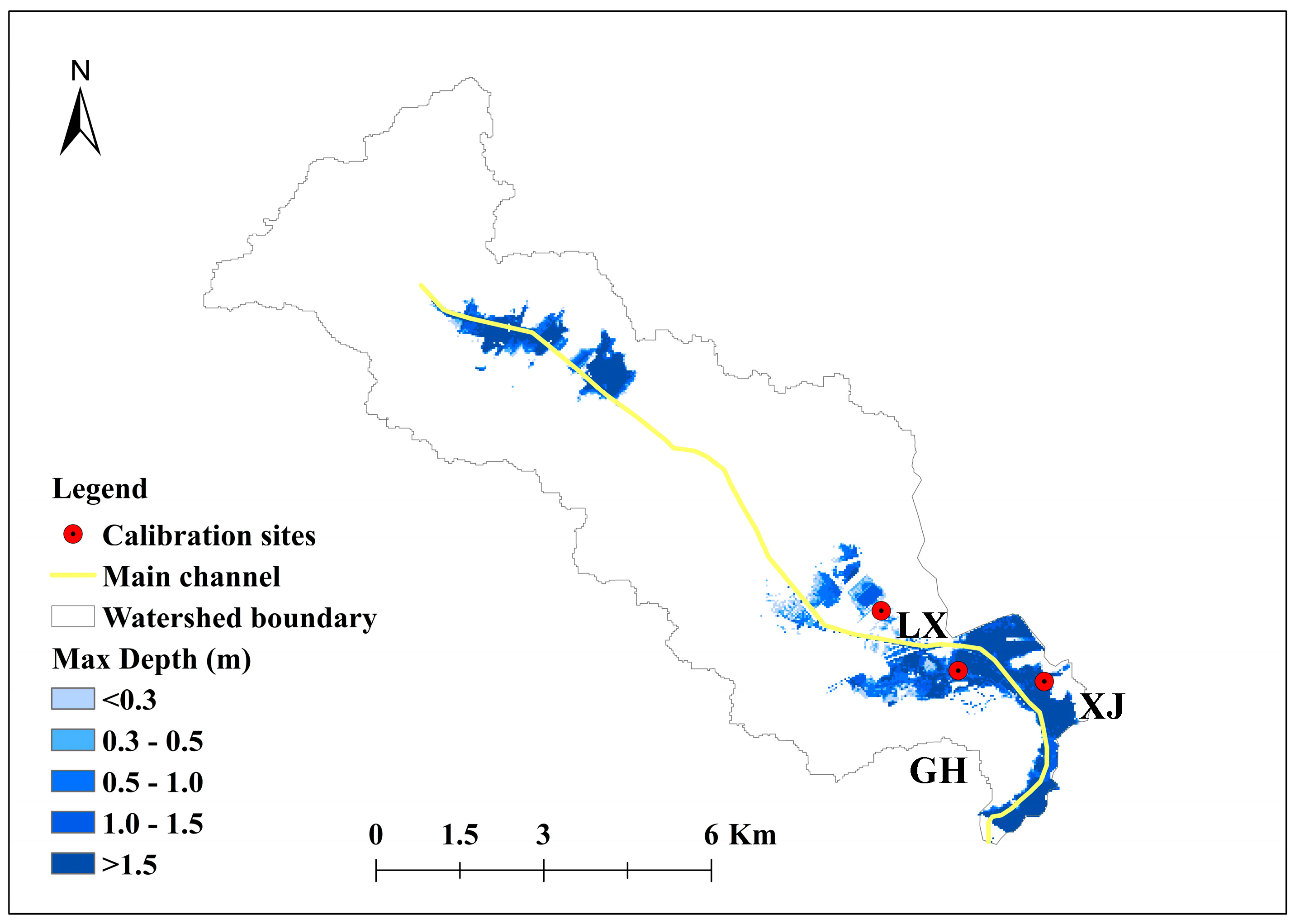
2.1. Study Area

The average annual precipitation in Guangzhou is approximately 1800 mm, which is unevenly distributed over time. More than 80% of the annual precipitation occurs during the rainy season from April to September [27]. Guangzhou is also influenced by semidiurnal mixed tides in Lingding Bay. Regarding land cover changes, the built-up area in Guangzhou has increased rapidly, from 297.5 km² in 2000 to 1380.6 km² in 2022.

The Yonghe River Watershed (YRW) is located to the east of the central urban area of Guangzhou, China (Figure 1). The YRW covers two metro stations, Guanhu and Xinsha, that were completely flooded on 22 May 2020 (Figure 2). Moreover, some communities and villages in the downstream area were severely flooded, to depths of >1.5 m.

The watershed covers a relatively small area of 63.8 km². The Yonghe River is 21.1 km long and originates from the hilly area in Huangpu District, flows through Zengcheng District, and ends at the East River, one of the main tributaries of the Pearl River. The percentage of impervious surfaces in the YRW increases from 13.9% in 2000 to 54.4% in 2020. The average slope of YRW is 5.71 degree and quartiles are 0.46, 2.06, 7.56, and 58.46 degrees.

2.2. Model Data

2.2.1. Topography

Accurate topography is critical in flood modeling because low-quality DEM data may lead to large uncertainties in the results, such as flooding area and inundation depth. The topographic data were acquired using airplane-based LiDAR, and the spatial resolution of the resulting DEM data was 2 m.

2.2.2. Land Cover

Land cover in 2020 was extracted from the Gaofen 1 Satellite image (multi-spectrum, 8 m spatial resolution) using an object-oriented classification approach. The classification results included water, vegetation, bare earth, and construction land. The overall accuracy was 97.7%, and the Kappa coefficient was 0.96.

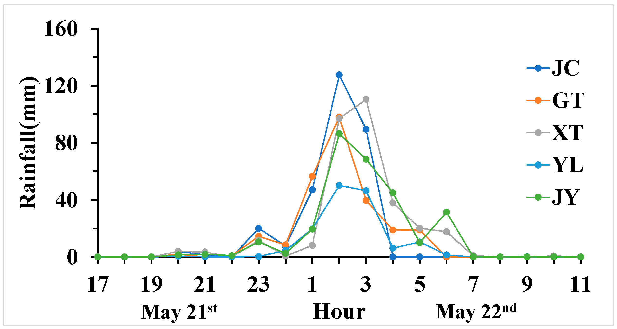
2.2.3. Rainfall and Tide Levels

Rainfall data were collected from the official website of the Water Resources Department of Guangdong Province (http://210.76.80.76:9001/Map/Map.aspx?id=2, accessed on 6 October 2020). In 2020, the storm event occurred from 8 p.m. on 21 May to 7 a.m. on 22 May and peaked at midnight (Figure 3). The entire watershed was divided into subareas based on the locations of the weather stations using the Thiessen polygon method. Rainfall depths at the five stations are listed in

Table 1. Total rainfall depth and maximum three-hourly rainfall depth of adjacent rain gauges.

Weather Station	Total Rainfall (mm)	Max Three-Hour Rainfall (mm)
Xintang (XT)	312.8	245.0
Jiancun (JC)	297.2	264.0
Jiuyu (JY)	278.5	200.0
Guangzhou Toyota (GT)	258.0	194.0
Yeling (YL)	140.1	116.0

.

At approximately the same time, the tidal level peaked (Figure 4). Huangpu was the nearest tide station to the study area, and tidal data from Huangpu during the storm event were collected from the National Marine Data and Information Service’s website (https://www.cnss.com.cn/tide/, accessed on 6 October 2020).

2.3. Model Setup

The flood process was modeled by coupling the Hydrologic Engineering Center’s Hydrologic Modeling System (HEC-HMS) and the River Analysis System (HEC-RAS). The study area was divided into multiple catchments, each of which had an outlet for the main channel to the Yonghe River. The HEC-HMS simulated the hydrological processes in each catchment and provided the flow rate at the outlets, which served as the boundary conditions for the HEC-RAS. To interact with ocean processes, the boundary conditions also included the tidal level. Finally, HEC-RAS simulated the overflow of floodwater along the main channel and calculated the flooded area and inundation depth using the simulated flood stage and high-quality terrain data.

2.3.1. HEC-HMS

Runoff generation was calculated using the Soil Conservation Service Curve Number (SCS-CN) method, in which only one parameter, CN, is required. For one catchment, the CN value equals the mean CN value of different land cover types weighted by area (Equation (1)).

$$\begin{array}{c}\overline{CN}=\frac{{\sum }_{i=1}^n{CN}_i{A}_i}{{\sum }_{i=1}^n{A}_i}\end{array}$$

(1)

where $\overline{CN}$ is curve number of the catchment, n is the number of land cover types in the catchment, and $A_i$ and ${CN}_i$ represent the area and curve, respectively, for the ith land cover type.

Runoff volumes generated in the catchments were routed to the catchment outlet using the SCS Unit Hydrograph approach, which has a principal parameter, lag time. The lag time can be defined as follows:

$$\begin{array}{c}Lag=\frac{l^{0.8}{\left(S+1\right)}^{0.7}}{517.217{\overline{Slp}}^{0.5}}\end{array}$$

(2)

where $Lag$ is the time (h), $l$ is the flow length (m) of the longest flow path, $\overline{Slp}$ indicates the average slope (%), and $S$ represents the maximum potential retention (mm), equal to $\left(1000/\mathrm{C}\mathrm{N}\right)-10$, where CN represents the number of SCS curves. The flow length and average slope can be obtained using the HEC-GeoHMS 10.7 software, which is a geospatial hydrology toolkit in ArcMap.

In the HEC-HMS model, the base flow was set as zero. The base flow in such a small watershed is limited and its impact on rainfall event simulations was represented by model calibration implicitly.

2.3.2. HEC-RAS

The geometric model of the Yonghe River was established based on a 2 m LiDAR DEM using HEC-GeoRAS, which is also a toolkit in ArcMap. Cross sections were defined at 100 m intervals along the main channel and cross-section lines were extended outwardly until watershed boundary. Floodplains lower than overflow water level are considered to be flooded. The energy loss comprised contraction or expansion and friction losses. The cross sections of the Yonghe River changed gradually, especially in the downstream areas. Thus, contraction and expansion coefficients were set to 0.1 and 0.3, respectively. The evaluation of friction losses required Manning’s roughness coefficients for the main channel and floodplains. Roughness coefficients were defined separately for the main channel, left floodplain, and right floodplain. The floodplains were empirically divided into upstream and downstream parts based on significant differences in land cover. The roughness values were determined during model calibration using the 22 May flood event.

2.4. Model Calibration

2.4.1. Inundation Depths

A field investigation was conducted on 25 May 2020 using surveying equipment, including the global navigation satellite system’s real-time kinematic (GNSS RTK) and total station equipment. GNSS RTK can determine the three-dimensional coordinates of a single point with centimeter precision. The key to accurate positioning is the real-time corrections that the equipment requires from a continuously operating reference station (CORS) system. When satellites are inadequately available due to blockages by buildings and canopies, the GNSS RTK cannot function well; then, the alternative is “GNSS RTK + total station”. The GNSS’s receiver was first moved to a position where accurate positioning was to be achieved. A total station was then used to survey the height difference between the flood mark and the GNSS receiver. Finally, the elevation of the floodmark above the 1985 National Elevation Datum was calculated using the height difference and GNSS RTK observations. In this manner, three sites were investigated, namely Guanhu Station, Xinjie Village (close to Xinsha Station), and Lixin Road (Figure 1b), and their inundation depths were observed to be 0.87, 1.65, and 1.0 m, respectively.

2.4.2. Roughness Coefficients

The roughness coefficients used for the model calibration are listed in

Table 2. Manning’s roughness coefficients for model calibration.

Subarea	Range	Number of Samples
Upstream left floodplain	0.011–0.080	4
Upstream right floodplain	0.011–0.080	4
Main channel	0.025–0.033	3
Downstream left floodplain	0.011–0.017	3
Downstream right floodplain	0.011–0.017	3

. The upstream floodplains exhibited a wider range of roughness coefficients; thus, more samples were collected from there. In total, 432 combinations of roughness coefficients were obtained.

2.4.3. Parameter Optimization

Each combination was input to simulate the 22 May flood event, and its performance was measured by the mean deviation (MD) of the simulated inundation depths from the observed inundation depths at the three sites considered in the field investigation, as follows:

$$\mathrm{M}\mathrm{D}=\frac{1}{3}{\sum }_{i=1}^3{|h}_{sim}\left(i\right)-h_{obs}\left(i\right)|$$

(3)

where $h_{sim}\left(i\right)$ and $h_{obs}\left(i\right)$ represent the simulated and observed inundation depths, respectively. The roughness coefficients with the lowest MD among all 432 combinations were applied for the subsequent scenario analyses.

The calibrated model was then applied to examine the responses of rainfall intensity, tidal level, and land cover change, and to identify the dominant flood mechanism in coastal watersheds.

2.5. Scenarios Design

2.5.1. Rainfall Scenarios

Since most of the precipitation from the 22 May event was concentrated over 3 h, rainfall scenarios were designed for a duration of 3 h. According to the local intensity–duration–frequency relationships released by the Guangzhou Bureau of Water Authority [28], the rainfall depths for typical return periods are listed in

Table 3. Average intensity and rainfall depth for 3 h designed storms with typical return periods in Guangzhou, China.

Return Period (Year)	Average Intensity (L/(ha.s))	Rainfall Depth (mm)
5	100.255	108.3
10	116.64	126.0
20	136.011	146.9
50	159.062	171.8
100	175.228	189.2

.

The rainfall depth for each return period was distributed over time by the Chicago curve [29], where the rising and falling limbs can be represented as:

$$q\left(t_b\right)=\frac{a\left[\frac{\left(1-n\right)t_b}{1-r}+b\right]}{{\left[\frac{t_b}{1-r}\right]}^{1+n}}$$

$$q\left(t_a\right)=\frac{a\left[\frac{\left(1-n\right)t_a}{r}+b\right]}{{\left[\frac{t_a}{r}+b\right]}^{1+n}}$$

$$a=167A_1\left(1+\mathrm{F}\times logT\right),$$

(4)

where q(t_b) and q(t_a) are the time series of rainfall intensity in the rising and falling limbs, respectively; t_b and t_a are the times before and after the peak rainfall intensity, respectively; r is the ratio of the peak rainfall intensity time to the total duration and was set to 0.33; A₁ is the rainfall depth (mm) for the one-year return period; F is the parameter of rainfall depth variation; T is the return period (year); b is used to adjust the rainfall duration; and n is related to rainfall attenuation. Parameters including F, b, and n were determined by calibration using historical rainfall events. The values of F, b, and n were 0.438, 11.259, and 0.750, respectively [28].

2.5.2. Tide Level Scenarios

The tide levels at the Huangpu Station for the five typical return periods [30] are listed in

Table 4. Tide levels for the five typical return periods at Huangpu Station based on the 1985 National Elevation Datum.

Return Period (Year)	2	10	20	50	100
Tide level (m)	2.47	2.81	2.96	3.16	3.30

. The tidal gauge station, marked in Figure 1a, is only 20 km away from the outlet of Yonghe River. As a result, the tidal processes at the outlet of Yonghe River can be represented by processes at the tidal gauge station. The tidal levels in Table 4 were directly applied as boundary conditions to the Yonghe River.

2.5.3. Land Cover Scenarios

Besides the 2020 land cover data, data from four additional years (2000, 2010, 2025, and 2035) were used. Land cover data for 2000 and 2010 were obtained from the Geographical Information Monitoring Cloud Platform (http://www.dsac.cn/DataProduct/Detail/200804, accessed on 6 October 2020), which provides high-resolution (30 m) land cover products with quality control. It has an overall accuracy greater than 85% for construction land and residential areas. Land cover for 2025 and 2035 (30 m spatial resolution) was predicted using the Future Land Use Simulation Model Software (FLUS 2.4) [31]. The FLUS model is an integrated model for multitype land-use scenario simulations that couples human and natural effects [32].

2.6. Perturbation Analysis

As rainfall intensity, tide level, and land cover imperviousness have different dimensions, the contribution of one influential factor can be measured by the relative change in flooding indicators, flooded area or inundation depth, divided by the relative change in the factor. First, a baseline scenario was set, i.e., 5-year design rainfall, 2-year design tide, and land cover in 2020. The model was then run by varying one factor and controlling for the other two. The relative change in the flood indicators can be defined as

$${\beta }_{result}=\frac{R_i-R_{base}}{R_{base}}$$

(5)

where ${\beta }_{result}$ is the relative change, and $R_{base}$ and $R_i$ are the model results for flooded area, and inundation depth under the baseline and perturbation scenarios, respectively. Similarly, the relative change in influential factors can be defined as

$${\beta }_{factor}=\frac{F_i-F_{base}}{F_{base}}$$

(6)

where ${\beta }_{factor}$ is the relative change, and $F_{base}$ and $F_i$ are influential factors under the baseline and perturbation scenarios, respectively.

The ratio ${\beta }_{result} / {\beta }_{factor}$ for one factor represented the measure of its impact on flooding. The larger the ratio, the more powerful the factor.

3. Results

3.1. Model Performance

In the model calibration, the best combination of roughness coefficients produced the smallest error of the mean inundation depth, 0.06 m (

Table 5. Model’s performance in the calibration.

Roughness Coefficient					Deviation of Inundation Depth (m)			Mean Deviation (m)
Upstream		Main Channel	Downstream		GH	XJ	LX
Left	Right		Left	Right
0.034	0.034	0.033	0.011	0.014	0.04	0.02	0.12	0.06

). The maximum inundation depth simulated using the best combination is shown in Figure 5. Compared with the upstream area, the downstream area was flooded more severely, and the inundation depth was more than 1.5 m in some places.

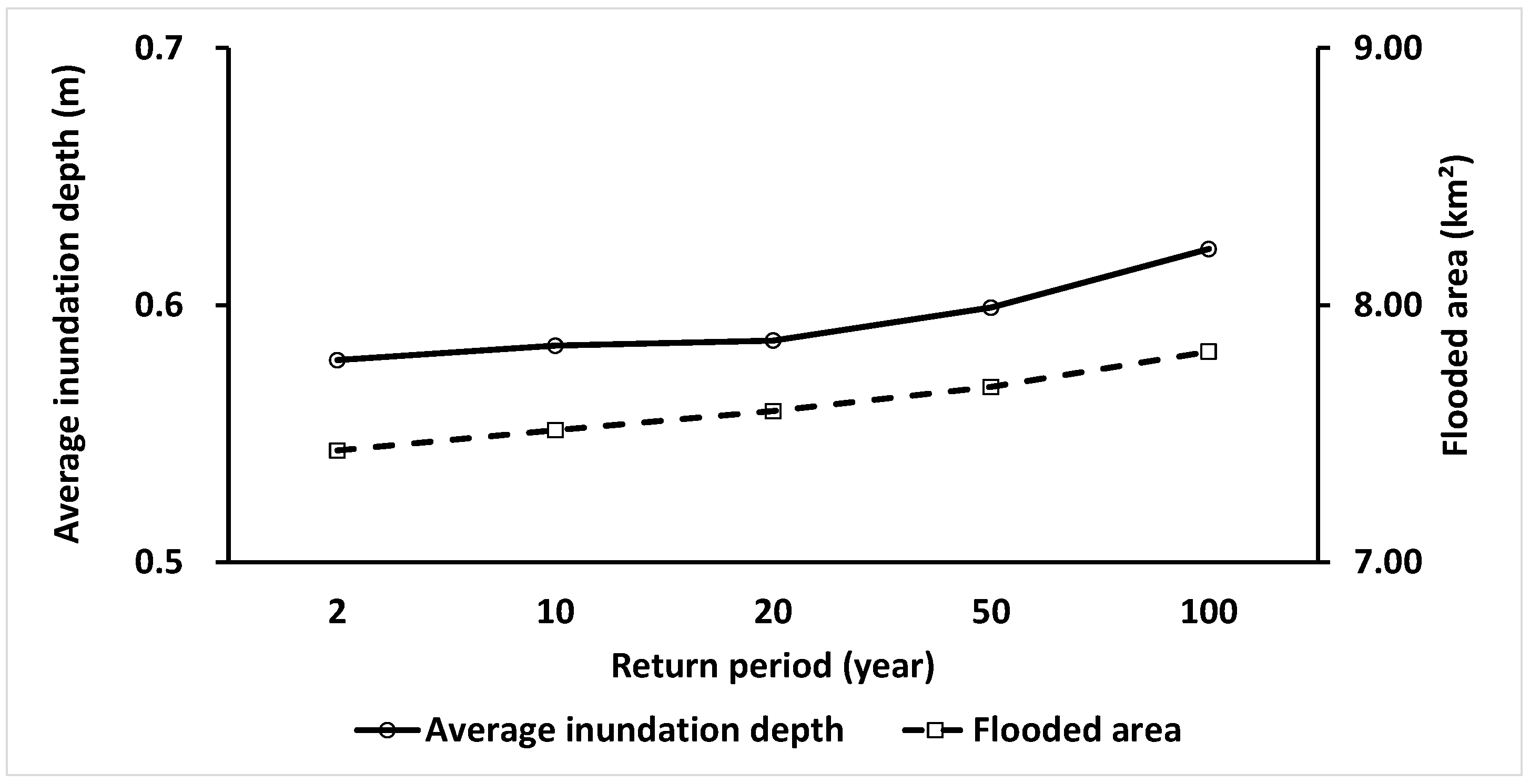
3.2. Responses to Rainfall Intensity Change

The model was run by varying the rainfall scenario based on the baseline scenario (5-year design rainfall, 2-year design tide, and land cover in 2020), and the two indicators, average inundation depth and flooded area, were computed for all scenarios (Figure 6). A significant monotonic increasing trend with return period was observed for both indicators. Average inundation depth increased significantly by 63.8%, from 0.58 m at 5-year scenarios to 0.95 m at 100-year scenarios. Flooded areas rose from 7.43 km² at 5-year scenarios to 12.97 km² at 100-year scenarios, showing a spatial expansion of 74.6%.

The increases in both the average inundation depth and flooded area exhibited nonlinear trends among the five return periods. The increase in inundation depth between the 5- and 20-year return periods (0.191 m) was larger than that between the 20- and 100-year return periods (0.176 m); similarly, increases in flooded areas were 2.986 km² between the 5- and 20-year return periods and 2.546 km² between the 20- and 100-year return periods, indicating a decrease in the rising rate.

3.3. Responses to Tide Level Change

The responses to tide levels are shown in Figure 7. Although the changes in the two indicators caused by variations in tide levels were much smaller than those in the rainfall scenarios, they also showed an increasing trend. Average inundation depth increased by 6.9%, from 0.58 m at 5-year scenarios to 0.62 m at 100-year scenarios. Flooded areas rose from 7.43 km² at 5-year scenarios to 7.82 km² at 100-year scenarios, with a spatial expansion of 5.2%.

Compared with rainfall intensity, the increase in both indicators due to tide level changes exhibited an opposite nonlinear trend. The increase in inundation depth between the 2- and 20-year return periods (0.008 m) was smaller than that between the 20- and 100-year return periods (0.036 m). Similarly, the increase in flooded areas was 0.153 km² between the 2- and 20-year return periods and 0.232 km² between the 20- and 100-year return periods, indicating an increase in the rate of increase.

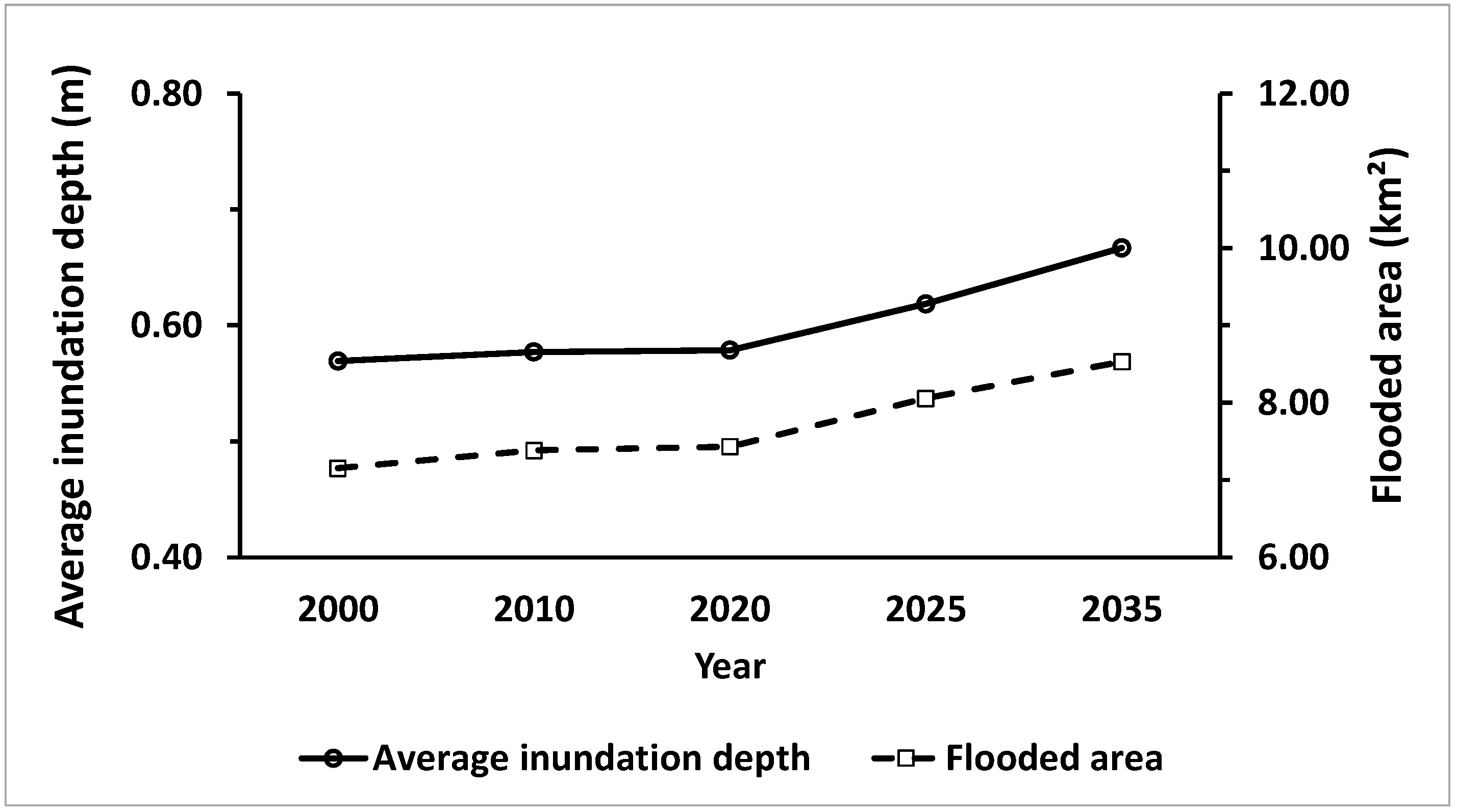
3.4. Responses to Land Cover Change

Due to rapid urbanization in the study area, the percentage of impervious land increased from 13.9% in 2000 to 54.4% in 2020 (

Table 6. Percentage of impervious surface from 2000 to 2035.

Year	Imperviousness			Annual Growth
	Upstream	Downstream	Total
2000	14.3%	13.2%	13.9%	-
2010	41.0%	63.3%	48.8%	3.5%
2020	42.3%	76.9%	54.4%	0.6%
2025	51.1%	81.0%	61.6%	1.4%
2035	58.5%	92.7%	70.4%	0.9%

); however, this number is predicted to further increase in the future. The land cover product of the FLUS model predicted imperviousness to increase by 61.6% in 2025 and 70.4% in 2035, which would be slower than that in the first decade of the 21st century. Since the urbanization process is spatially heterogeneous in watersheds, the downstream area would be occupied at a faster pace than the upstream area.

Flood responses to land cover changes are shown in Figure 8. The magnitude of change in flood indicators was between those in the rainfall- and tide-level scenarios. Both indicators showed an overall increasing trend. Average inundation depth increased by 17.2%, from 0.57 m in 2000 to 0.67 m in 2035. Flooded areas rose from 7.15 km² in 2000 to 8.53 km² in 2035, with a spatial expansion of 19.3%. Responses to land cover changes exhibited nonlinear trends like the responses to the tide levels. The rate of increase during 2020–2035 was found to be larger than that during 2000–2020, while the increase in inundation depth between 2000 and 2020 (0.009 m) was smaller than that between 2020 and 2035 (0.088 m). Increases in flooded area were 0.28 km² and 1.1 km² for 2000–2020 and 2020–2035, respectively, suggesting a stronger turn in the rising rate than the nonlinear trend in the responses to tide level.

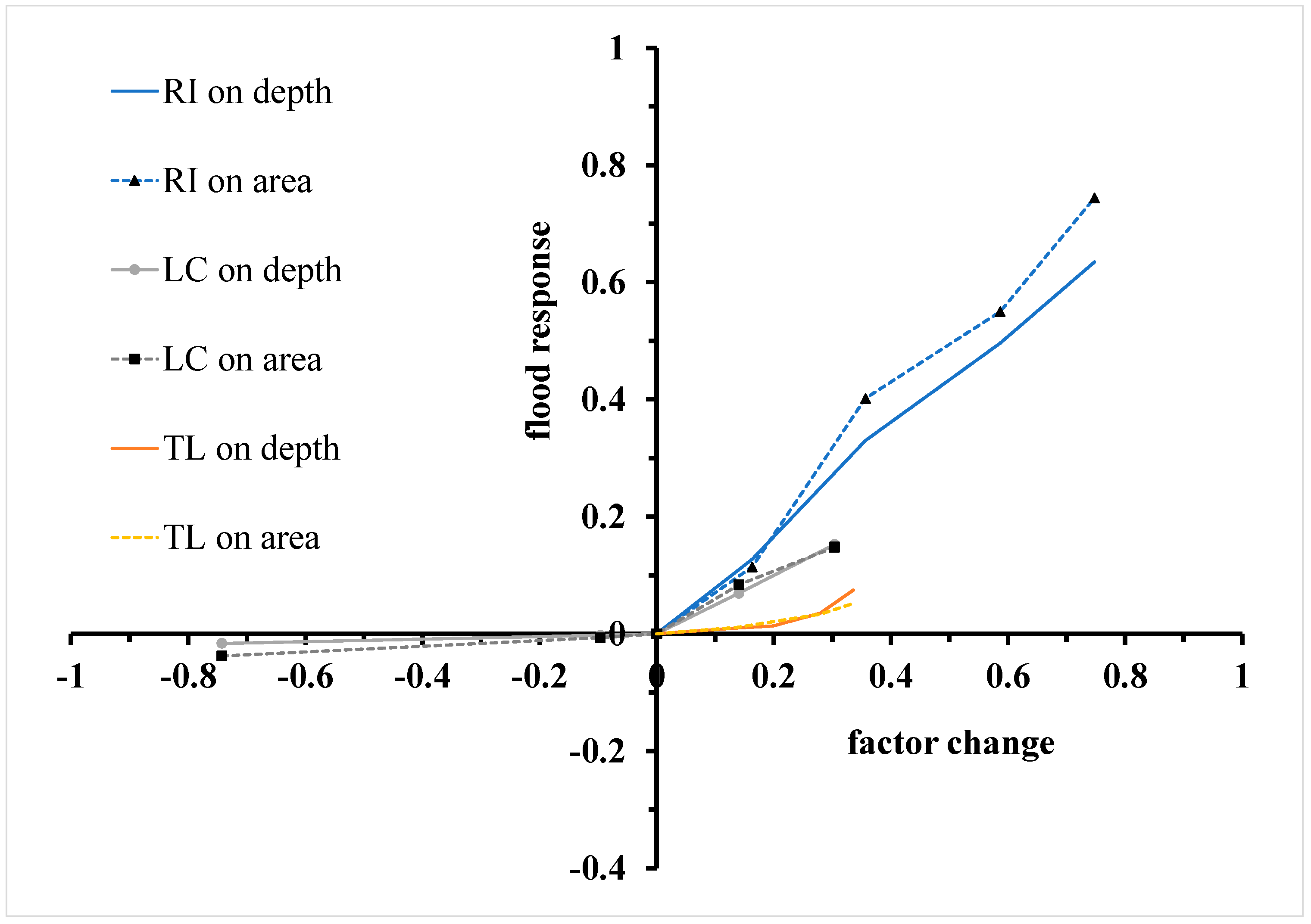
3.5. Comparison of Nonlinear Responses

Since changes in a single factor in the given scenarios did not show an equal rate of change in other factors, the analysis of a single factor cannot reveal the responses precisely. Instead, a perturbation analysis based on the baseline scenarios, 5-year design rainfall, 2-year design tide, and land cover in 2020 was conducted to compare the influences of the three factors on the flooding indicators. The results are shown in Figure 9.

The impact of a factor can be represented by the slope, which is defined as the relative change in the flood response divided by the relative change in the factor (

Table 7. Slopes for responses to rainfall intensity, land cover, and tide level. S1–S5 denote the five scenarios designed for a given factor. For example, rainfall intensity scenarios S1, S2, S3, S4, and S5 correspond to 5-, 10-, 20-, 50-, and 100-year return periods, respectively. Phase S1–S2 denotes response change from 5- to 10-year return periods. The depth and area represent the average inundation depth and flooded area, respectively.

Phase	Rainfall Intensity		Land Cover		Tide Level
	Depth	Area	Depth	Area	Depth	Area
S1–S2	0.78	0.70	0.02	0.05	0.07	0.08
S2–S3	1.05	1.49	0.03	0.07	0.06	0.16
S3–S4	0.72	0.64	0.49	0.60	0.27	0.16
S4–S5	0.86	1.21	0.51	0.39	0.70	0.33
Overall S1–S5	0.85	1.00	0.50	0.49	0.22	0.15

). Generally, both flooding indicators were most influenced by rainfall intensity, followed by land cover and tide levels. Considering the curve segments that connect the designed scenarios, considerable variations can be observed in the slope of the segments in each curve. The rainfall intensity curve varied the least among segments, whereas the other two curves showed stronger nonlinearity, increasing faster for larger values of factor. The curve corresponding to land cover could be divided into two phases according to the scenario of 2020, suggesting that the considered watershed is currently at a critical point regarding land cover imperviousness, after which the flood risk will increase rapidly. The curves of tide level showed strong rising trends in the last phase, S4–S5, with slope of 0.70 (flood depth) and 0.33 (flood area). The impact of the tide level at extreme tides was greater than, or at least comparable to, land cover change. Considering the continuously rising sea level and the accelerating global water cycle, the negative impact of tides may increase.

If a diagonal line starting from the original point is drawn in the upper right portion, most curves are under the line, suggesting that relative changes in influential factors do not induce the same amount of relative changes in flood depth and flood area. A probable reason for these outcomes is depth–area–volume relationship of detention areas such as floodplains, which could be simplified as circular cones. If water is continuously added to a circular cone, increases of water area and water depth triggered by a constant volume show a declining trend. Moreover, curve shapes are subject to floodplain topography.

4. Discussion

4.1. Impact of Tides on River-Dominated Watersheds

According to the model analysis, compound flooding in the Yonghe River was primarily dominated by precipitation, and this conclusion is consistent with previous studies on the Pearl River Delta (PRD), where flood discharges dominated the flood stages in the middle and upper PRD, while storm surges had the maximum impact near the river mouth [33]. Since the YRW is located in the upper part of the PRD, the impact of tides in this region is smaller than that near the river mouth. Nevertheless, the increase in tidal impacts should receive more attention in long-term policymaking. Qiu et al. [34] reported that extreme sea level has been the dominant driver of compound coastal–fluvial flooding in the PRD over the past 60 years, and its impact is projected to rise with global warming in the future.

In the past two decades, multiple typhoons have caused record-breaking storm surges at the mouth of the Pearl River, leading to severe damages to coastal cities in Guangdong, such as Zhuhai, Shenzhen, and Guangzhou. For example, at almost all hydrological stations near the Pearl River mouth, water levels recorded by Mangkhut (No. 1822) and Hato (No. 1713) ranked first and second in the history since hydrological records became available, respectively. In Zhongda Station, the three largest water levels were 8.28 m in 2018 (Mangkhut, 1822), 7.79 m in 2017 (Hato, 1713), and 7.73 m in 2008 (Hagupit, 0814). At Dashi Station, corresponding water levels were 8.19 m in 2018, 7.95 m in 2017, and 7.79 m in 2008. These new extreme records have significantly changed the probability distribution of the water levels, thus reducing the return period of storm tides.

Similar studies have been conducted in other regions. An analysis in Haikou, a city in southern China, showed that the return period of storm tides was reduced by 10.3% under the nonstationary scenario [25]. Unusual long-distance inland propagation can be observed in the Yangtze River [26] and the Mississippi River [22]. Extreme tidal levels under the nonstationary scenario will cause small- and medium-sized watersheds to face greater flood hazards than ever before.

In summary, flood risk management in coastal watersheds that are currently river-dominated should also consider the impact of tides, particularly for extreme water levels. As suggested in this study, the flood risk increases faster at high tide levels owing to the nonlinear feature of the flood response to the tide.

4.2. Timing for Flood Risk Management in Developing Regions

Flood risk management measures, particularly engineering measures, require substantial financial support, which is even more challenging for developing regions that struggle to balance multiple criteria, including economic growth, pollution control, disaster reduction, etc. The demand and supply of flood risk management are always imbalanced, which further amplifies flood risk by simultaneously increasing hazards and exposure. Rapid changes in land cover are the main reason for the increase in flood risk in developing regions. First, the transformation from a natural landscape to construction or residential land not only leads to losses in natural infiltration and detention capacity but also reduces surface roughness. Consequently, it increases the magnitude of flood discharge and leads to earlier peak timing, exacerbating the flood hazards. Second, the continuous growth of population and industry significantly increases exposure to floods, creating a new demand for flood protection.

The Environmental Kuznets Curve (EKC) provides a reference guide for the timing of flood risk management. The EKC was initially developed to describe the relationship between economic progress and environmental degradation over time as an economy progresses. The curve is an inverted U-shape, in which pollution increases with initial development but declines with further economic progress. Under this framework, the YRW was found to be at a turning point currently. As of 2020, more than half of the area was covered by impermeable surfaces, and metro systems have stretched to this area, suggesting that its socioeconomic condition has grown adequately. In contrast, the flood control capability of levees (less than a 10-year return period) and the design standard of the drainage system (approximately a 1-year return period) in this area are insufficient. Furthermore, the nonlinear flood responses to land cover changes (Table 7) confirm that increases in construction land in the future will increase the risk of flood hazards.

Based on the analysis conducted in this study, 50% imperviousness is recommended as an indicator of the urgent demand for flood risk management measures in small watersheds. A previous study in the Yangtze River Delta [35] explored the impact of urbanization on floods in a basin with a 1371 km² area and found that urbanization impacts can be better understood at the sub-basin level. Suburban areas may experience a high flood risk with urbanization expansion, even though the impact at the basin level may not be remarkable. Taking Guangzhou as an example, its built-up area in 2022 was 1380.6 km², which accounted for 18.56% of the total area of 7434.4 km². However, highly developed small watersheds such as the YRW are expected to face flood hazards more severe than ever before. The findings of the study on the PRD are consistent with conclusions at the sub-basin level in the Yangtze River Delta. The results for these two world-class delta regions are informative for recognizing the optimal timing for flood risk management in other small coastal watersheds.

4.3. Uncertainties and Limitations

First, the hydrodynamic model did not include the drainage process. During urbanization, the agricultural landscape was transformed into a mixture of manufacturing plants, newly built residential communities, and original villages and farmlands. The design standard for drainage in this suburban area is lower than that in the downtown areas. Moreover, this is quite common in villages where drainage depends mainly on overland flow. The exclusion of the drainage process is likely to impact simulations with small return periods but has limited influence on scenarios with large return periods.

Second, the model was calibrated using only the flood marks without timestamps. Without other events for validation, the model may be overfitted and, thus, its ability to generalize may be questioned. This concern can be largely addressed by the fine-scale data used in this study, including topography and land cover. In addition, the absence of flood peak time may produce uncertainties in model calibration. It should be noted that flood depth is time-dependent. If a hydrograph is used for model calibration, deviation of flood peak time would reduce the model performance significantly. Nevertheless, in a small watershed like YRW, flood processes are quick and, thus, it is acceptable to calibrate a model only with maximum flood depth.

Third, the roughness parameters remained unchanged among the five land cover scenarios, which is likely to underestimate the nonlinearity of flood responses. In the first (2000) and second (2010) land cover scenarios, using roughness parameters from the 2020 scenario likely overestimated flood responses. In contrast, underestimation may have occurred in future land cover scenarios (2025 and 2035). Consequently, the nonlinearity of flood responses to land cover change was underestimated to some extent. However, only one flood event was available for model calibration; thus, the roughness parameters for the other four scenarios could not be precisely determined.

Finally, this study does not include the impact of climate changes, which are influencing rainfall intensity and tide level across the globe. As mentioned in Section 4.1, record-breaking tide levels have already reduced the return periods. The impact is the same for rainfall intensity. Based on model results in this study and climate change trends, it can be anticipated that tide level will have a continuously rising impact on flood hazard from a long-term perspective.

4.4. Benefits and Future Work

Population and economic growth in coastal regions create an urgent demand for flood risk regulation measures. According to China’s statistical yearbooks, the shares of coastal provinces in the total population were 41.33%, 43.25%, and 45.05% in 2000, 2010, and 2020, respectively, showing a clear move towards coastal areas. Furthermore, coastal provinces have accounted for 76.22% of the net population increase over the past two decades. Regarding the economy, the gross domestic product (GDP) of coastal provinces increased from USD 7894 trillion in 2000 to USD 76,703 trillion in 2020, presenting nearly a tenfold expansion.

The conclusions on the nonlinear flood responses are an important reminder for small watersheds that have not experienced extreme flood events like the one that occurred on 22 May 2020. According to incomplete statistics, out of more than 50,000 small- and medium-sized river watersheds in China, 85% are located along the coasts of river basins [36]. Compared with the significantly enhanced flood prevention in the main rivers, small- and medium-sized river watersheds are weak points in flood risk management systems. Approximately 70–80% of flood-related losses in China are caused by floods in small- and medium-sized watersheds [37].

In developing regions, the lack of hydrological data is common, making it difficult to understand flood mechanisms and assess the intensity of future flood hazards. Although extreme flood events, such as the 22 May 2020 flood in Guangzhou, opened a window to understanding flood mechanisms, the rare occurrence of extreme events makes them infeasible for most watersheds. In future research, small watersheds should be classified into limited groups using machine learning techniques based on environmental factors and socioeconomic conditions. Thus, knowledge learned from limited extreme events can be transferred to other data-scarce small watersheds to enhance future flood risk management. In addition, the impact of climate changes should be incorporated to produce possible future flood hazard scenarios.

5. Conclusions

Compound flooding caused by multiple drivers simultaneously or in close succession poses a challenge to flood risk management in coastal regions owing to nonlinear interactions among drivers. Rapid land cover change leads to an increase in peak discharge and an advance in peak time; therefore, it plays a significant role in flood risk management in developing coastal regions. This study investigated the nonlinear responses of compound floods to rainfall intensity, tide levels, and land cover changes in a developing coastal watershed in Guangzhou, China, which is currently undergoing rapid urbanization. Regarding the impact on inundation depth and flood area, the most influential factor was rainfall intensity, followed by land cover change and tide level. Flood responses to all three factors showed a nonlinear increasing pattern but with different rates of increase. The response curves of the tidal level and land cover change increased faster at high values, whereas the rainfall intensity curve varied slightly. These findings highlight the importance of integrating tidal impacts into flood risk management even in river-dominated coastal watersheds.

In this study, the transfer of learned knowledge was discussed. Currently, the extreme water levels and long-distance inland propagation of storm surges are creating larger flood hazards in small watersheds, which are further amplified by rapid urbanization. Based on the findings of this study, 50% imperviousness is recommended to be used as an indicator of the urgent demand for flood risk management measures in small watersheds.

Additionally, this study had some limitations. First, the model did not incorporate the drainage process, which may have led to uncertainties in the simulation of small return periods. Second, the model was not validated after calibration because of a lack of historical flood data. Third, the analysis of the simulation results did not consider the probability of the co-occurrence of different drivers. Therefore, in future research, nonlinear flood responses should be tested across multiple spatial scales by considering additional combinations of drivers and their co-occurrence probabilities. Furthermore, knowledge learned from extreme flood events regarding environmental factors and socioeconomic conditions should be transferred to similar watersheds selected by machine learning techniques.

References

1. UNDRR (United Nations Office for Disaster Risk Reduction). Human Cost of Disasters: An Overview of the Last 20 Years 2000–2019. 2020. Available online: https://www.undrr.org/publication/human-cost-disasters-overview-last-20-years-2000-2019 (accessed on 12 March 2021).
2. IPCC (Intergovernmental Panel on Climate Change). Climate Change 2021: The Physical Science Basis; IPCC: Geneva, Switzerland, 2021. [Google Scholar]
3. Couasnon, A.; Eilander, D.; Muis, S.; Veldkamp TI, E.; Haigh, I.D.; Wahl, T.; Winsemius, H.C.; Ward, P.J. Measuring compound flood potential from river discharge and storm surge extremes at the global scale. Nat. Hazards Earth Syst. Sci. 2020, 20, 489–504. [Google Scholar] [CrossRef]
4. Hendry, A.; Haigh, I.D.; Nicholls, R.J.; Winter, H.; Neal, R.; Wahl, T.; Joly-Laugel, A.; Darby, S.E. Assessing the characteristics and drivers of compound flooding events around the UK coast. Hydrol. Earth Syst. Sci. 2019, 23, 3117–3139. [Google Scholar] [CrossRef]
5. Wahl, T.; Jain, S.; Bender, J.; Meyers, S.D.; Luther, M.E. Increasing risk of compound flooding from storm surge and rainfall for major US cities. Nat. Clim. Chang. 2015, 5, 1093–1097. [Google Scholar] [CrossRef]
6. Ward, P.J.; Couasnon, A.; Eilander, D.; Haigh, I.D.; Hendry, A.; Muis, S.; Veldkamp TI, E.; Winsemius, H.C.; Wahl, T. Dependence between high sea-level and high river discharge increases flood hazard in global deltas and estuaries. Environ. Res. Lett. 2018, 13, 084012. [Google Scholar] [CrossRef]
7. Wu, W.; McInnes, K.; O’Grady, J.; Hoeke, R.; Leonard, M.; Westra, S. Mapping Dependence Between Extreme Rainfall and Storm Surge. J. Geophys. Res.-Ocean. 2018, 123, 2461–2474. [Google Scholar] [CrossRef]
8. Zellou, B.; Rahali, H. Assessment of the joint impact of extreme rainfall and storm surge on the risk of flooding in a coastal area. J. Hydrol. 2019, 569, 647–665. [Google Scholar] [CrossRef]
9. Zheng, F.; Westra, S.; Leonard, M.; Sisson, S.A. Modeling dependence between extreme rainfall and storm surge to estimate coastal flooding risk. Water Resour. Res. 2014, 50, 2050–2071. [Google Scholar] [CrossRef]
10. Gori, A.; Lin, N.; Smith, J. Assessing Compound Flooding from Landfalling Tropical Cyclones on the North Carolina Coast. Water Resour. Res. 2020, 56, e2019WR026788. [Google Scholar] [CrossRef]
11. Zhang, Y.; Ye, F.; Yu, H.C.; Sun, W.L.; Moghimi, S.; Myers, E.; Nunez, K.; Zhang, R.Y.; Wang, H.; Roland, A.; et al. Simulating compound flooding events in a hurricane. Ocean. Dyn. 2020, 70, 621–640. [Google Scholar] [CrossRef]
12. Nasr, A.A.; Wahl, T.; Rashid, M.M.; Camus, P.; Haigh, I.D. Assessing the dependence structure between oceanographic, fluvial, and pluvial flooding drivers along the United States coastline. Hydrol. Earth Syst. Sci. 2021, 25, 6203–6222. [Google Scholar] [CrossRef]
13. Ghanbari, M.; Arabi, M.; Kao, S.; Obeysekera, J.; Sweet, W. Climate Change and Changes in Compound Coastal-Riverine Flooding Hazard Along the US Coasts. Earths Future 2021, 9, e2021EF002055. [Google Scholar] [CrossRef]
14. Bevacqua, E.; Maraun, D.; Vousdoukas, M.I.; Voukouvalas, E.; Vrac, M.; Mentaschi, L.; Widmann, M. Higher probability of compound flooding from precipitation and storm surge in Europe under anthropogenic climate change. Sci. Adv. 2019, 5, eaaw5531. [Google Scholar] [CrossRef]
15. Faccini, F.; Luino, F.; Paliaga, G.; Roccati, A.; Turconi, L. Flash Flood Events along the West Mediterranean Coasts: Inundations of Urbanized Areas Conditioned by Anthropic Impacts. Land. 2021, 10, 620. [Google Scholar] [CrossRef]
16. Fang, J.; Wahl, T.; Fang, J.; Sun, X.; Kong, F.; Liu, M. Compound flood potential from storm surge and heavy precipitation in coastal China: Dependence, drivers, and impacts. Hydrol. Earth Syst. Sci. 2021, 25, 4403–4416. [Google Scholar] [CrossRef]
17. Didier, D.; Baudry, J.; Bernatchez, P.; Dumont, D.; Sadegh, M.; Bismuth, E.; Bandet, M.; Dugas, S.; Sevigny, C. Multihazard simulation for coastal flood mapping: Bathtub versus numerical modelling in an open estuary, Eastern Canada. J. Flood Risk Manag. 2019, 12, e12505. [Google Scholar] [CrossRef]
18. Bakhtyar, R.; Maitaria, K.; Velissariou, P.; Trimble, B.; Mashriqui, H.; Moghimi, S.; Abdolali, A.; Van der Westhuysen, A.J.; Ma, Z.; Clark, E.P.; et al. A New 1D/2D Coupled Modeling Approach for a Riverine-Estuarine System Under Storm Events: Application to Delaware River Basin. J. Geophys. Res.-Ocean. 2020, 125, e2019JC015822. [Google Scholar] [CrossRef]
19. Bilskie, M.V.; Hagen, S.C. Defining Flood Zone Transitions in Low-Gradient Coastal Regions. Geophys. Res. Lett. 2018, 45, 2761–2770. [Google Scholar] [CrossRef]
20. Santiago-Collazo, F.L.; Bilskie, M.V.; Hagen, S.C. A comprehensive review of compound inundation models in low-gradient coastal watersheds. Environ. Model. Softw. 2019, 119, 166–181. [Google Scholar] [CrossRef]
21. Cai, H.Y.; Savenije HH, G.; Toffolon, M. Linking the river to the estuary: Influence of river discharge on tidal damping. Hydrol. Earth Syst. Sci. 2014, 18, 287–304. [Google Scholar] [CrossRef]
22. Feng, D.; Tan, Z.; Engwirda, D.; Liao, C.; Xu, D.; Bisht, G.; Zhou, T.; Li, H.; Leung, L.R. Investigating coastal backwater effects and flooding in the coastal zone using a global river transport model on an unstructured mesh. Hydrol. Earth Syst. Sci. 2022, 26, 5473–5491. [Google Scholar] [CrossRef]
23. Juarez, B.; Stockton, S.A.; Serafin, K.A.; Valle-Levinson, A. Compound Flooding in a Subtropical Estuary Caused by Hurricane Irma 2017. Geophys. Res. Lett. 2022, 49, e2022GL099360. [Google Scholar] [CrossRef]
24. Savenije HH, G.; Toffolon, M.; Haas, J.; Veling EJ, M. Analytical description of tidal dynamics in convergent estuaries. J. Geophys. Res. 2008, 113, C10025. [Google Scholar] [CrossRef]
25. Xu, H.; Zhang, X.; Guan, X.; Wang, T.; Ma, C.; Yan, D. Amplification of Flood Risks by the Compound Effects of Precipitation and Storm Tides Under the Nonstationary Scenario in the Coastal City of Haikou, China. Int. J. Disaster Risk Sci. 2022, 13, 602–620. [Google Scholar] [CrossRef]
26. Guo, L.; Zhu, C.; Wu, X.; Wan, Y.; Jay, D.A.; Townend, I.; Wang, Z.B.; He, Q. Strong Inland Propagation of Low-Frequency Long Waves in River Estuaries. Geophys. Res. Lett. 2020, 47, e2020GL089112. [Google Scholar] [CrossRef]
27. Yang, L.; Scheffran, J.; Qin, H.; You, Q. Climate-related flood risks and urban responses in the Pearl River Delta, China. Reg. Environ. Change 2015, 15, 379–391. [Google Scholar] [CrossRef]
28. GBWA (Guangzhou Bureau of Water Authority). The Rainstorm Formula and Calculation Chart in Guangzhou Downtown; GBWA: Guangzhou, China, 2011. [Google Scholar]
29. Keifer, C.J.; Chu, H.H. Synthetic Storm Pattern for Drainage Design. J. Hydraul. Div. 1957, 83, 1–25. [Google Scholar] [CrossRef]
30. Wang, X. Storm Surge Disaster Risk Assessment and Impact Forecasting Research. Ph.D. Thesis, Wuhan University, Wuhan, China, 2016. [Google Scholar]
31. Zhao, L.; Liu, X.; Liu, P.; Chen, G.; He, J. Urban Expansion Simulation and Early Warning based on Geospatial Partition and FLUS Model. J. Geo-Inf. Sci. 2020, 22, 517–530. [Google Scholar]
32. Liu, X.; Liang, X.; Li, X.; Xu, X.; Ou, J.; Chen, Y.; Li, S.; Wang, S.; Pei, F. A future land use simulation model (FLUS) for simulating multiple land use scenarios by coupling human and natural effects. Landsc. Urban Plan. 2017, 168, 94–116. [Google Scholar] [CrossRef]
33. Wang, X.; Guo, Y.; Ren, J. The Coupling Effect of Flood Discharge and Storm Surge on Extreme Flood Stages: A Case Study in the Pearl River Delta, South China. Int. J. Disaster Risk Sci. 2021, 12, 495–509. [Google Scholar] [CrossRef]
34. Qiu, J.; Liu, B.; Yang, F.; Wang, X.; He, X. Quantitative Stress Test of Compound Coastal-Fluvial Floods in China’s Pearl River Delta. Earth’s Future 2022, 10, e2021EF002638. [Google Scholar] [CrossRef]
35. Zhou, F.; Xu, Y.; Chen, Y.; Xu, C.Y.; Gao, Y.; Du, J. Hydrological response to urbanization at different spatio-temporal scales simulated by coupling of CLUE-S and the SWAT model in the Yangtze River Delta region. J. Hydrol. 2013, 485, 113–125. [Google Scholar] [CrossRef]
36. Zhao, Q.; Zhu, Y.; Wan, D.; Yu, Y.; Lu, Y. Similarity Analysis of Small- and Medium-Sized Watersheds Based on Clustering Ensemble Model. Water 2020, 12, 69. [Google Scholar] [CrossRef]
37. Li, H.; Wang, R.; Huang, Q.; Xiang, J.; Qin, G. Advances on Flood Forecasting of Small-Medium Rivers. J. China Hydrol. 2020, 40, 16–23. [Google Scholar]
Figure 1. Study area location (a) and landscape (b). Huangpu (HP) and Zengcheng (ZC) are the two districts in eastern Guangzhou. The field survey sites A, B, and C represent Lixin Road, Guanhu Station, and Xinjie Village, respectively. Rain gauges in and around the study area include Jiancun (JC), Jiuyu (JY), Yeling (YL), Guangzhou Toyota (GT), and Xintang (XT). The watershed is empirically divided into upstream and downstream areas by the red solid line. The landscape image was taken from the Gaofen 1 Satellite in 2020.
Land 12 01743 g001
Figure 2. Guanhu Metro Station during (a) and post (b) the flood. The photo (a) was taken on 22 May 2020, and sourced from Weibo, a public social media platform in China. The photo (b) was captured by the research team on 25 May 2020, when a rescue team was pumping flood water out from the metro station.
Land 12 01743 g002
Figure 3. Temporal distribution of rainfall depth at rain gauges in and around the study area.
Land 12 01743 g003
Figure 4. Water levels at Huangpu Tide Station under the National Elevation datum of 1985 from 21 May to 22 May.
Land 12 01743 g004
Figure 5. Simulated maximum inundation depths at Lixin Road (LX), Guanhu Station (GH), and Xinjie village (XJ) for the flood event on 22 May 2020.
Land 12 01743 g005
Figure 6. Average inundation depth and flooded area under rainfall scenarios in typical return periods.
Land 12 01743 g006
Figure 7. Average inundation depth and flooded area under tide level scenarios in typical return periods.
Land 12 01743 g007
Figure 8. Average inundated depth and inundated area under different land cover scenarios.
Land 12 01743 g008
Figure 9. Influence of three influential factors (rainfall intensity, tide level, and land cover change) on average inundation depth and flooded area.
Land 12 01743 g009