Article

Optimizing Management of the Qinling–Daba Mountain Area Based on Multi-Scale Ecosystem Service Supply and Demand

1
School of Tourism, Henan Normal University, Xinxiang 453007, China
2
School of Geography and Tourism, Shaanxi Normal University, Xi’an 710119, China
*
Author to whom correspondence should be addressed.
Land 2023, 12(9), 1744; https://doi.org/10.3390/land12091744
Submission received: 3 August 2023 / Revised: 30 August 2023 / Accepted: 5 September 2023 / Published: 8 September 2023
(This article belongs to the Special Issue Exploring Urban Landscape Sustainability)

Abstract

:
Accurately identifying the supply and demand of ecosystem services at multiple scales and determining the factors that influence the supply–demand relationship are crucial for guiding the sustainable management and restoration of regional ecosystem services. In view of this, we quantified the supply and demand of five ecosystem services at multiple scales in the Qinling–Daba Mountain area based on spatial and statistical data, exploring the relationships between the supply and demand for ecosystem services at multiple scales and examining the mechanisms by which factors like natural and human activities affect the evolution of the supply and demand patterns of these services. The results show that (1) there was no risk associated with supply and demand of ESs in the Qinling–Daba Mountain area, and numerous ESs were in excess. The impact of ES supply and demand became increasingly clear as the spatial scale was increased. (2) Under multiple spatial scales, the relationship between the supply and demand of ESs will change. At the mesoscale, the relationship between ES supply and demand was the most significant, whereas at the macroscale, the relationship between ES demands was the most significant. (3) Cultivated land, grass land, and forest land are the key land use categories in regional ecosystem service hotspots, providing richer ecosystem service functions for the region. (4) Precipitation and NDVI are the main elements determining the supply of ecosystem services. While GDP and population density have a significant impact on the demand for ecosystem services, natural causes are primarily responsible for trade-offs in ecosystem services. This study aims to evaluate the supply–demand relationship and driving factors of multiple scale in the Qinling–Daba Mountains, providing a scientific basis for the sustainable management of ecosystems in the region.

1. Introduction

Ecosystem service supply refers to the physically available natural resources and services that ecosystems provide [1]. Moreover, the demand for ecosystem services is the quantity and quality of ecosystem services needed or desired by society [2,3]. Together, these two components constitute the dynamic process of ecosystem service flow from natural ecosystems to human social systems [4]. The continuous supply of ecosystem services forms the basis for sustainable regional development. However, due to increasing human activities, two-thirds of the global supply of ecosystem services has declined [5]. With advancements in urbanization, people’s demand for ecosystem services has been increasing [6], resulting in the compactness of urban ecosystem services and exacerbating the imbalance between supply and demand of ecosystem services in both urban and rural areas. This poses a serious threat to the health of ecosystems and the sustainable development of human societies. Therefore, understanding the relationship between ecosystem service supply and demand at different scales and their driving mechanisms is a prerequisite for sustainable ecosystem service management and can help improve human well-being [7].
The composition of components and hierarchical structure within different ecosystems varies, determining the hierarchical complexity, spatial variability, and multidimensional scale-dependence of landscape patterns, ecological processes, and ecological functions; i.e., the scale effect for ecosystem services [8,9]. Scale effects are an important component of scale research, which is used to evaluate and understand the impacts of scale changes on the ecosystem structure, function, and their inter-relationships. Existing studies have found significant scale effects in the spatial distribution, trade-offs, and synergies of different types of ecosystem services [10,11,12]. Turner et al. (2014) studied 11 ecosystem services in Denmark at different spatial scales and found that cultures, such as vegetation carbon sequestration, tourism, and recreation, were clustered and distributed at a spatial scale of 50 km, while provisioning services such as livestock quantity, food output, and freshwater output were clustered and distributed at a spatial scale of 150 km [13]. Zwierzchowska et al. (2018) conducted a multi-scale assessment of the cultural ecosystem services of urban parks in Central Europe and found that the parks’ ecosystem service capacities had advantages in attracting tourists at different scales that offset simple transportation inconvenience and distance [14]. Ciftcioglu (2023) found regional variability in the social valuation of agroecosystems by stakeholders at different scales [15]. Due to their scale-dependent nature, ecosystem service supply and demand patterns change with changing scales. On the one hand, the supply and demand of multiple ecosystem services may change at different spatial scales. For example, in Catalonia, Spain and the Ningxia Hui Autonomous Region in China, the degree of spatial matching between the supply and demand of some types of ecosystem services varies with scale, while in Quebec, Canada, the supply and demand of ecosystem services also show basic similarities at two smaller spatial scales while showing differences at a larger spatial scale [16,17,18]. Meanwhile, the structure, processes, and functions of the involved ecosystem service supply and demand vary at different spatial scales and influence the supply and demand of multiple ecosystem services through cascading effects [19]. At present, many scholars have begun to pay attention to the impact of the spatial scale on the supply and demand of ecosystem services. However, according to different scale management objectives, quantifying the scale variability of the supply and demand relationship of various ecosystem services at different scales and constructing a comprehensive supply and demand assessment that integrates multiple spatial scales and service types still remains a challenge.
Current research primarily focuses on assessing the supply and demand of ecosystem services; however, there is limited exploration of the underlying mechanisms that drive the balance between supply and demand. The balance between the supply and demand of ecosystem services is influenced by both natural and human factors [20]. Natural factors refer to the inherent properties of ecosystems that determine the formation and spatial distribution of ecosystem services. For example, in Eastern Australia, elevation, rainfall, temperature, and forest structure are the main determinants of ecosystem service provisioning in tropical forests [21]. Similarly, climate, soil, and vegetation are crucial in regulating climate services in the Americas [22]. In addition, human factors such as population size, socio-economic status, and agricultural development also affect the spatial distribution of ecosystem services. Increased human demand can lead to changes in ecosystem functions, including soil conservation, water yield services, food services, and biodiversity [23,24]. However, whether human factors have a positive or negative impact on ecosystem services depends on scientific planning [25]. Exploring ecosystem service drivers from multiple perspectives, including supply, demand, and the supply–demand balance, and implementing rational regional planning can effectively mitigate conflicts between economic development and ecosystems [26].
The Qinling–Daba Mountain area is crucial to China’s geographic pattern, functioning as a large-scale east–west ecological corridor. It boasts a rich variety of natural plant and animal resources thanks to its complex, diverse, and unique natural environment. However, due to the region’s abundant natural resources and poor economic conditions, there is often a mismatch between the supply and demand of ecosystem services. This mismatch can lead to contradictions and challenges in meeting the needs of ecosystem services [27]. Therefore, it is necessary to study the pattern of ecosystem services and changes in the supply and demand in the Qinling–Daba Mountain area. Previous research conducted by scholars has highlighted the importance of ecosystem services such as carbon sequestration, habitat quality, water yield services, soil conservation, and landscape aesthetics in the Qinling–Daba Mountain area. Previous research has primarily focused on comprehensive research on supply, regulation, support, and cultural services, with less attention given to specific services. However, due to the uncertainty of many research methods and the challenges in obtaining high-precision data in the previous period, there is a need for further investigation. Additionally, existing studies have predominantly focused on economically developed areas, neglecting economically underdeveloped and ecologically fragile areas [28]. Therefore, it is crucial to conduct research on the supply–demand balance and spatial correlation patterns of ecosystem services in poverty-stricken areas. This research can provide valuable insights into regional ecological asset compensation and serve as a scientific basis for promoting the rapid development of the local ecology and economy [29].
This study investigates the effects of scale on the supply and demand of ecosystem services, as well as the mechanisms driven by ecosystem services. It also provides recommendations for promoting sustainable management of mountain ecosystems. The research objectives were as follows: (1) to select five key ecosystem services that significantly affect local human development and evaluate their supply and demand at three different scales (macro, meso, and micro); (2) to quantify and spatialize the relationship between these five ecosystem services at multiple scales and analyze the correlation between their supply and demand using Spearman’s correlation coefficient; (3) to apply multiple hotspot analyses to examine the impacts of land use changes on ecosystem service provision and analyze the spatial patterns of surplus and deficit hotspots; (4) to use geographical detectors to analyze the drivers of ecosystem service supply and demand, as well as the trade-off relationships, in order to lay the foundation for optimal management of mountain ecosystems. This study aims to enhance our understanding of the matching of ecosystem services (ESs) across multiple scales. It also seeks to analyze the influencing factors of different ecosystem services and explore measures to alleviate supply and demand imbalances in different parts of the study area. Ultimately, the study aims to achieve sustainable development of ES.

2. Study Area and Methods
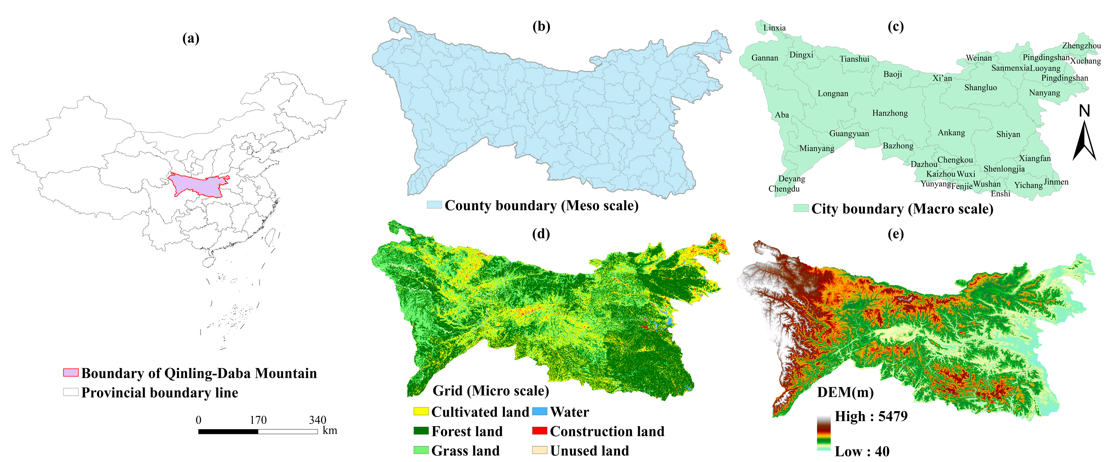
2.1. Study Area

The Qinling–Daba Mountain (30°50′~34°59′ N, 102°54′~112°40′ E) spans a total area of approximately 22,300 km2 and is situated in the Middle West of China. It encompasses Shaanxi Province, Gansu Province, Sichuan Province, Hubei Province, He-nan Province, and Chongqing city (Figure 1) [30,31]. The region exhibits diverse climate types, characterized by significant vertical changes. These include the northern subtropical marine climate, the subtropical warm temperate transitional monsoon climate, and the warm temperate continental monsoon climate. The average annual precipitation ranges from 450 to 1300 mm. Additionally, the region is known as the birthplace of several rivers, namely the Huaihe River, Hanjiang River, Danjiang River, and Luohe River. It boasts a well-developed water system, abundant runoff resources, and a forest coverage of 53%. This area in China is recognized as an important ecological functional area for biodiversity and water conservation. It boasts a wide range of mineral resources and natural gas reserves. Additionally, the region is abundant in tourism resources, indicating significant potential for development. This paper focuses on the regional characteristics of the Qinling–Daba Mountain and examines five ecosystem services: net primary productivity (NPP), water yield (WY), habitat quality (HQ), soil conservation (SC), and landscape aesthetics (LA). This study aims to analyze the spatial and temporal dynamics of the supply and demand patterns of these ecosystem services at different scales. Specifically, we analyze them at the grid (microscale), county (mesoscale), and city (macroscale) levels.

2.2. Data Sources

The data used in this study mainly include remote sensing data, land use data, vegetation type data, meteorological data, and statistical data. The data details and sources are shown in Table 1.
Data Description: In order to elucidate the relationship between various ecosystem services and supply–demand differences at different scales, the spatial resolution of the data was unified at 1 km. The microscale resolution was based on a 1 km grid as the research scale. The mesoscale resolution was based on the county scale as the research unit; therefore, the data were obtained through spatial statistics on a 1 km grid scale. The macroscale resolution was based on the city scale as the research unit, and the data acquisition was the same as the mesoscale reolution.

2.3. Supply and Demand Assessment of ESs

In order to accurately evaluate ESs, we utilized the evaluation model to measure the supply and demand indicators of each ES. Table 2 presents the quantitative methods and references for all the services. A comprehensive explanation of the quantification of services can be found in Appendix A.

2.4. Supply–Demand Ratio of ESs

In this study, the researchers utilized the supply–demand ratio of ecosystem services (ESDR) to analyze the combination of ecosystem service supply and demand. This approach helps to uncover the existing differences between supply and demand within the region [32].
E S D R = S D ( S m a x + D m a x ) / 2
In this formula, ESDR > 0 means that the supply of ecosystem services is greater than the demand, ESDR = 0 is the balance of supply and demand, and ESDR < 0 indicates that the supply is less than the demand. S and D represent the supply and demand of the ecosystem services, respectively.

2.5. Driver Analysis

The geographical detector model is used to identify the interactions between multiple factors by proposing a ‘factor force’ metric combined with GIS spatial overlay technology and set theory [45,46]. In this study, we applied this model to explore and measure the influence of different drivers on ecosystem services in the Qinling–Daba Mountain. The calculation formula used in this study was as follows:
q = 1 m = 1 n N m R m N R 2 2
In the formula, q represents the degree of influence of the driver on ESs, ranging from 0 to 1. A higher value of q indicates a greater influence of the driver on ESs, while a lower value suggests a smaller influence. When q = 0, it means that the driver does not affect the spatial distribution of ESs, and when q = 1, it means that the driver completely controls the spatial distribution of ESs. Here, m represents the class of driver, n represents the number of drivers, Nm and R represent the quality of the ESs for the regional sub region m and the entire region, respectively. Additionally, Rm2 and R2 represent the dispersive variance of the quality of ESs for the region m and the entire region.

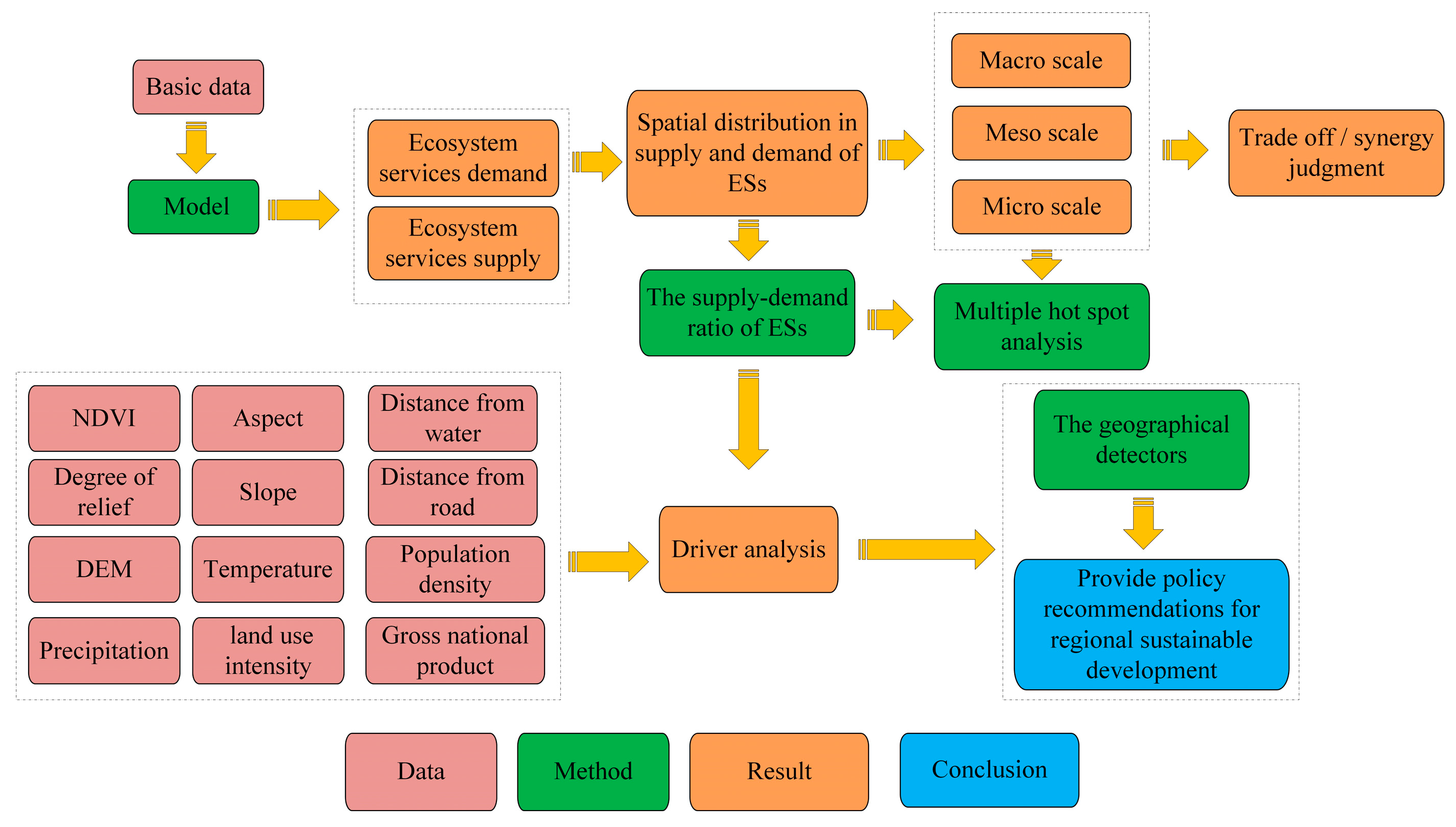
2.6. Methodological Framework

Aiming to study the characteristics of ecosystem management at different scales, this study evaluated the supply and demand of five ecosystem services in the Qinling–Daba Mountain region at the macro-, meso-, and microscales. On this basis, the study analyzed the synergistic relationship between the five ecosystem services and the trade-offs between supply and demand, as well as the spatial pattern of the surplus hotspots and deficit hotspots of the ecosystem services. Additionally, it analyzed the driving factors of the ecosystem services supply, demand, and trade-offs by using the geographical detectors model. This study can provide managers of all levels with a scientific basis for the development and utilization of natural ecosystems and help to ultimately achieve the goal of sustainable management. The research framework is shown in Figure 2.

3. Results

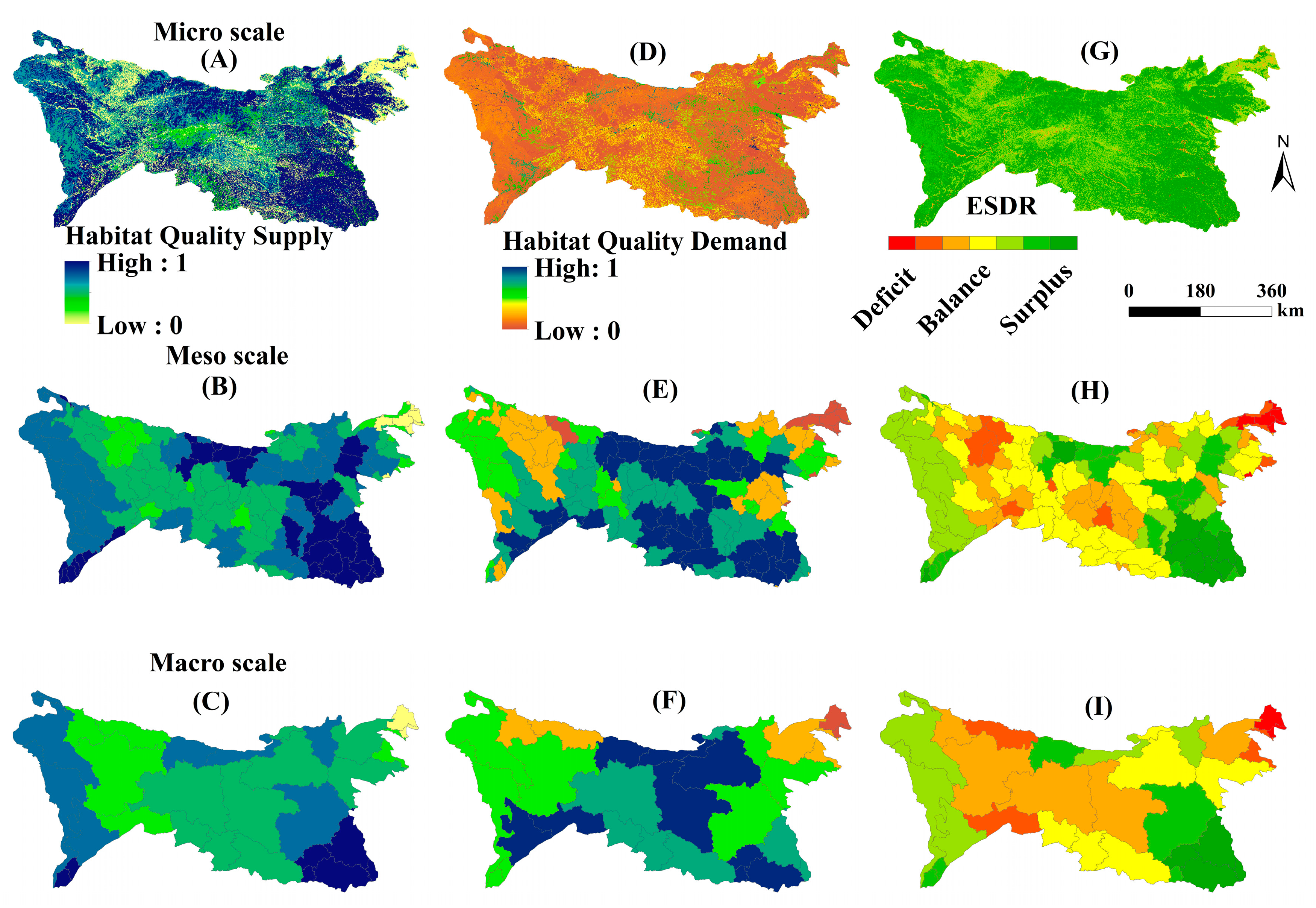
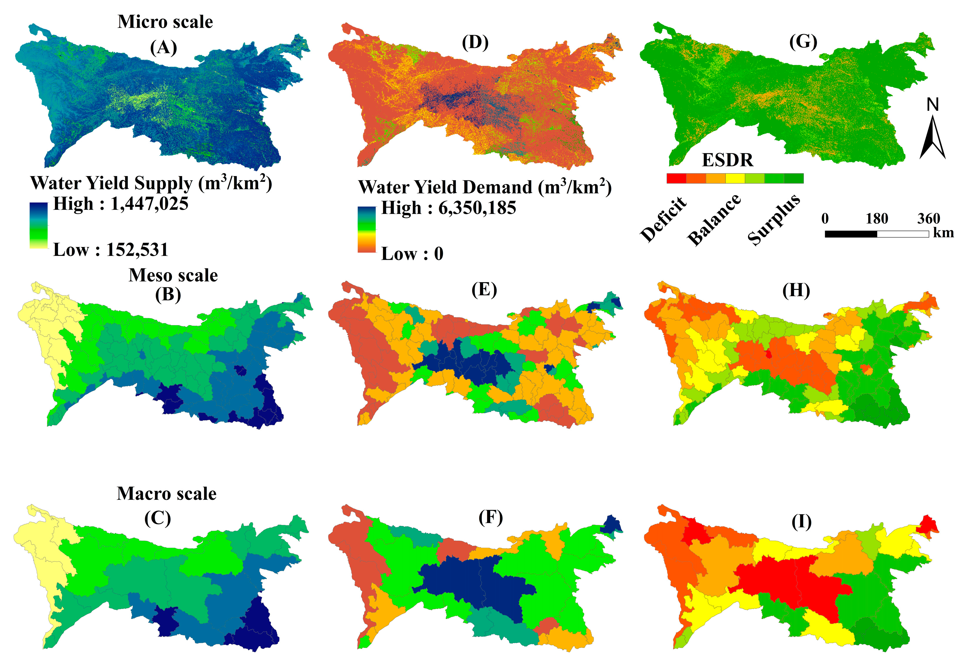
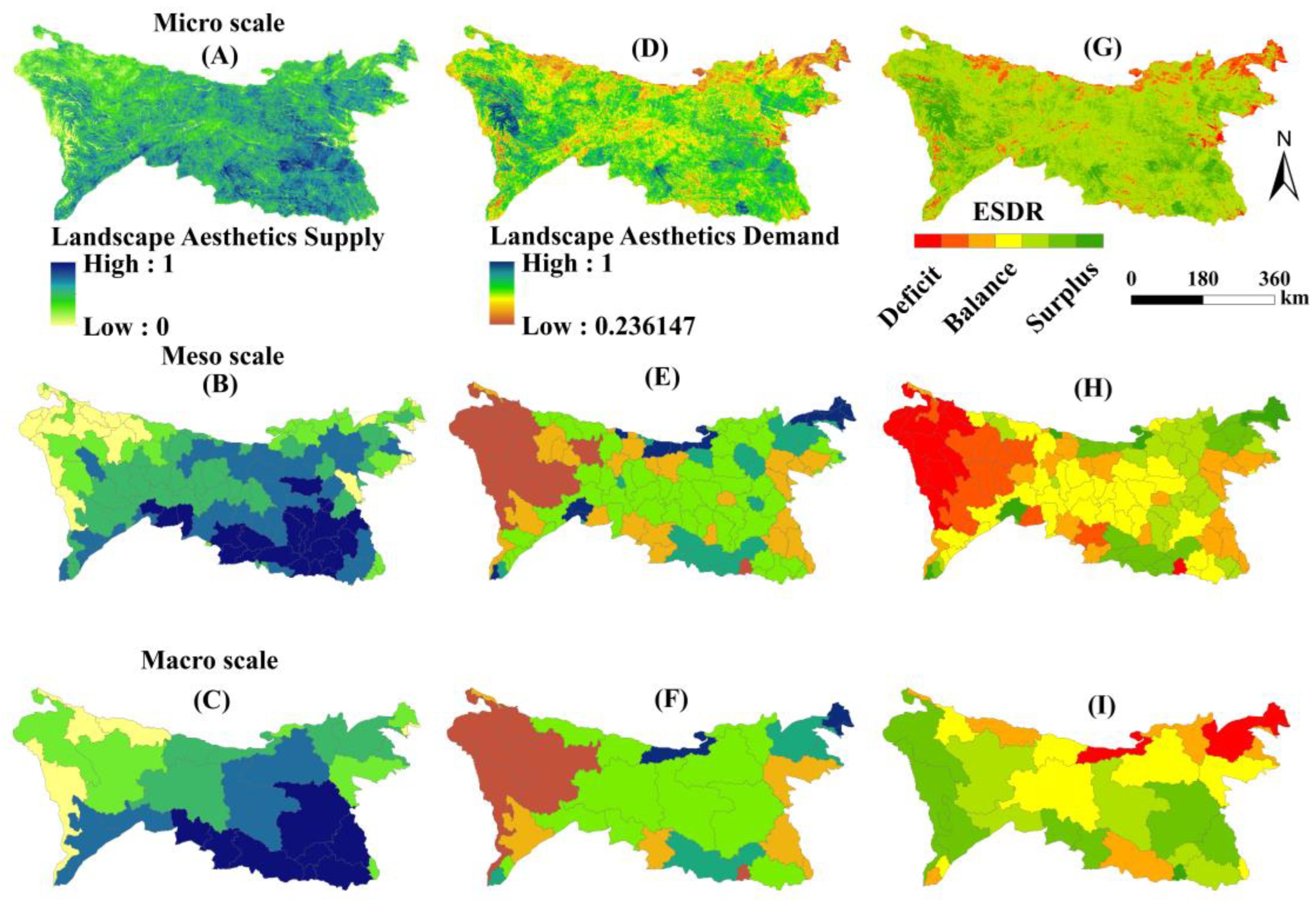
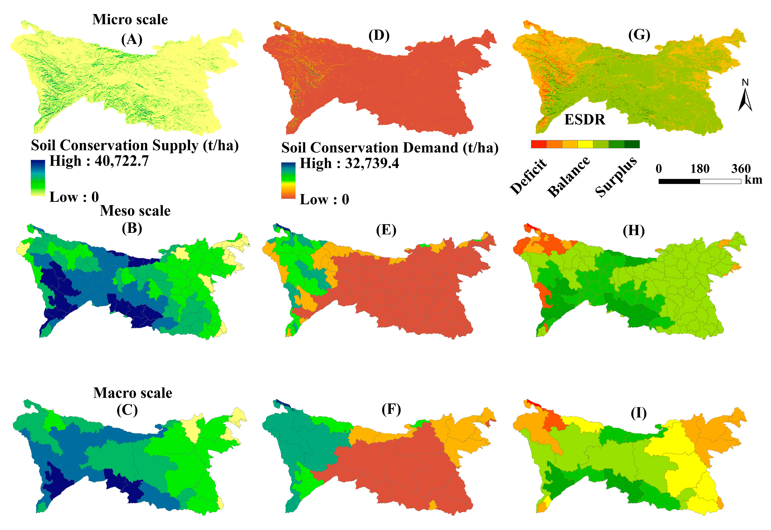
3.1. Supply and Demand Assessment of Ecosystem Services

This study assessed the NPP supply, demand, and supply/demand ratio in the Qinling–Daba Mountain at three different scales (Figure 3). The spatial distribution of supply at these three scales was generally similar, with high-value areas primarily concentrated in the northern and southern regions of the main Qinling Mountains and the Daba Mountains. In addition, lower values were observed in areas such as the Hanzhong Basin and the Nanyang Basin (Figure 3A–C). As the scale increases, the size of the high-value area gradually increases. The spatial difference in demand becomes more apparent across the three scales, primarily due to human activities. As the scale gradually increases, the high-demand area also expands, mainly concentrated in the central part of the study area and the eastern part of the Nanyang Basin area, where urban development is more advanced and human activities are frequent (Figure 3D–F). Furthermore, the spatial distribution maps of NPP at the three scales of ESDR (Figure 3G–I) indicate that the supply exceeds the demand in most areas, with a higher surplus around the edges than the middle, which aligns with the supply trend. However, when the scale changes to the macroscale, only Zhengzhou City in the eastern region exhibits higher demand than supply, resulting in a deficit in ESDR.
The spatial distribution of habitat quality in terms of supply and NPP exhibited similarities. Areas with high vegetation indices not only had higher NPP values but also provided richer habitat quality (Figure 3). The western region, characterized by higher elevation and low human damage, demonstrated high habitat quality (Figure 4A–C). In terms of demand, there was a trend of low values in the center and high values around the perimeter (Figure 4D–F). The distribution of high-value areas was more dispersed, mainly concentrated around the city, which had a higher population density. Moreover, only a small number of image elements of ESDR experienced a deficit at the microscale, while the rest were in surplus (Figure 4G). At the meso- and macroscales, the spatial change pattern was even more evident, with the supply of habitat quality in the study area being higher than the demand, resulting in a surplus for the entire region (Figure 4H,I).
The spatial distribution of water yield strongly correlated with precipitation, with a gradual decrease from south to north. The highest water yield was observed in the southeastern part of the study area, followed by the central region, while the western grasslands had the lowest water yield (Figure 5A–C). Similarly, the spatial distribution of water supply showed consistency across all three scales. Regarding the water demand, it was found to be higher in the central and northeastern parts of the study area, gradually decreasing towards the periphery. As the scales became coarser, areas with higher water demand gradually expanded (Figure 5D–F). Furthermore, the maps depicting the spatial distribution of water yield at the three scales of the ESDR (Figure 5G–I) revealed that most areas had a sufficient water supply. At the mesoscale, only one county exhibited a greater demand than supply, while all the other regions had a surplus of water supply, with the degree of surplus increasing from southeast to northwest, mirroring the trend observed in the water supply.
The spatial distribution of landscape aesthetic services exhibited similar patterns across the three scales. The values of landscape aesthetic services ranged from low to high, with the northwestern grasslands having lower values than the eastern forests (Figure 6A–C). The areas with high aesthetic value were concentrated in the southeastern part of Sichuan Province, while the low-value areas were found in mountainous regions with higher elevations. In terms of demand, the central and northeastern parts of the study area had a higher demand for landscape aesthetic services (Figure 6D–F), and there was greater spatial differentiation in the distribution of these services. Furthermore, the spatial distribution maps of landscape aesthetics at the three scales of the ESDR (Figure 6G–I) showed distinct variations, with deficit areas primarily located in the northern and central fragmented regions. At the mesoscale, the region as a whole had an oversupply of landscape aesthetic services (Figure 6H). At the macroscale, regions surrounding Zhengzhou City in the southern Shaanxi Province and Henan Province had an oversupply, while all the other regions had a surplus of these services (Figure 6I). It was found that there was spatial variability in the supply–demand ratio at the meso- and macroscales, with the western part of the region showing a deficit at the mesoscale and a surplus at the macroscale, mainly because the western part of the region is a high-value area in terms of its supply capacity at the macro scale. Meanwhile, the supply capacity was low at the mesoscale, resulting in spatial and scale variability in the regional supply–demand ratio.
The spatial distribution of soil conservation supply services is closely related to natural conditions such as precipitation, vegetation, and slope, gradually increasing from northeast to southwest. The high-value area is concentrated in the southwest, located in the Daxue Mountain and Minshan Mountain areas, and has a middle-subtropical climate with a high altitude, homogenous biodiversity, good conditions of original vegetation (seldom damaged), and high soil conservation. From the micro- to macroscales, the low-value area of soil conservation gradually becomes smaller, and the low-value area is mainly concentrated around Zhengzhou in the Henan Province (Figure 7A–C). The spatial variability in the demand was more obvious, and the spatial distribution tended to be higher in the west and east–west. From the micro- to macroscales, the high-value areas of soil retention gradually become larger (Figure 7D–F). In addition, the spatial distribution maps of soil retention at the three scales of the ESDR (Figure 7G–I) indicate that the middle region has a surplus, and the surrounding area is in a deficit stage. At the mesoscale, the southwest region has more demand than supply, and the all other regions have more supply than demand. At the macroscale, the region as a whole has a higher supply than demand, but Zhengzhou City and Xuchang City in Henan Province are in a deficit situation with negative supply/demand ratios.

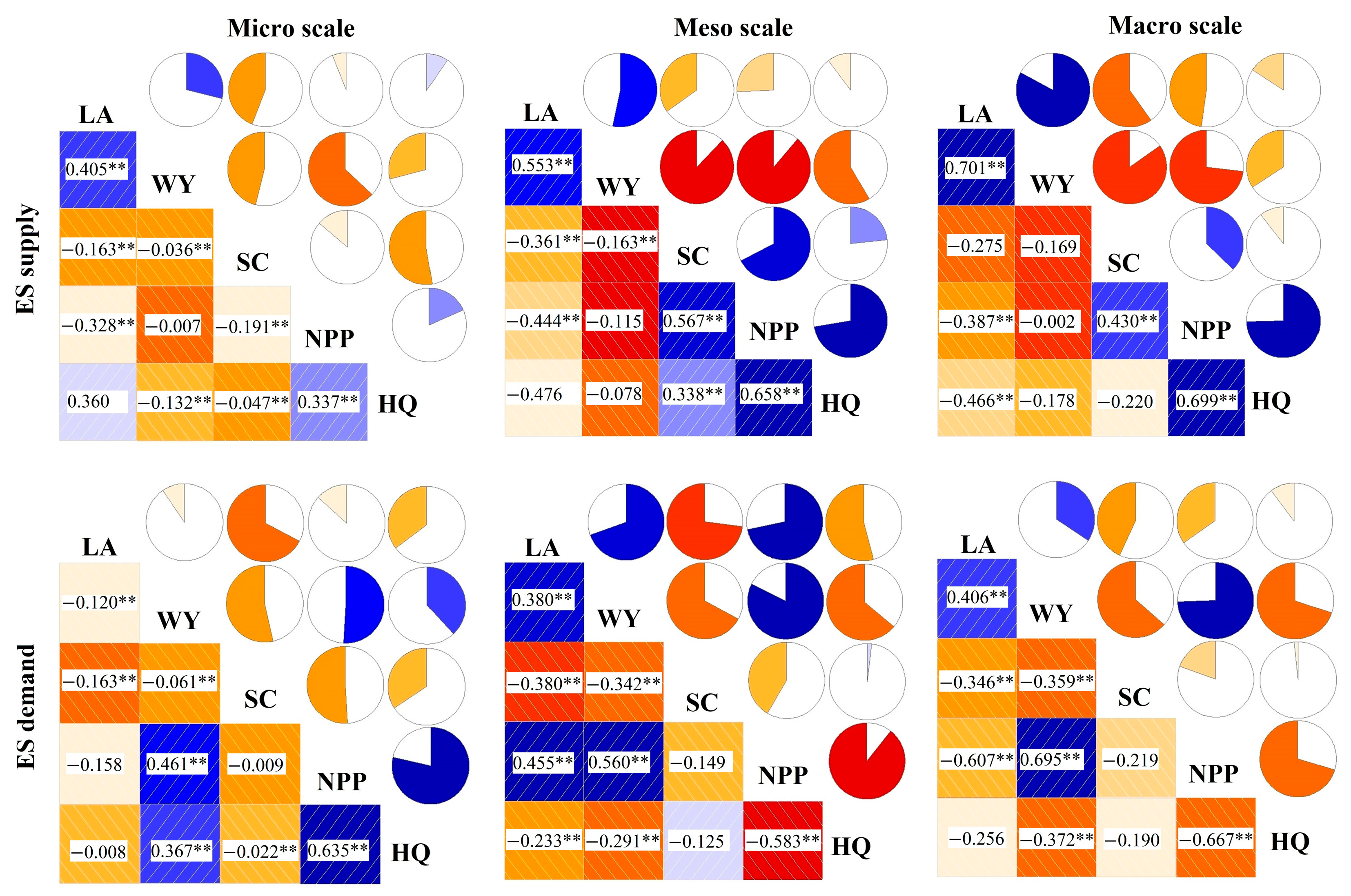
3.2. Interactions between ES Supply and Demand at Different Scales

3.2.1. Analysis of Ecosystem Service Tradeoffs

A correlation analysis revealed significant correlation variations between ecosystem services in the Qinling–Daba Mountain region. The spatial distribution exhibited a pattern of synergistic relationships around the perimeter and tradeoffs in the middle (Figure 8). Specifically, there were similar spatial distributions of synergistic relationships between NPP and HQ, LA, and SC. The high values were concentrated in the Fushun Mountain region and the western part of the Qinling Mountain range. This can be attributed to the strong regional dependence of NPP, dense vegetation, favorable growth conditions in mountainous areas, and the positive impact of increased vegetation cover on the quality of NPP. The tradeoff areas of water yield and HQ, LA, and SC were primarily concentrated in the central part of the region. This is mainly due to the dominance of cultivated vegetation, the arid climate, and poor vegetation growth conditions in this region. Moreover, the relationship between LA, SC, and HQ was more complex and varied across different regions. The synergistic relationship was mainly observed in mountainous areas with higher elevation, where human activities have less impact on the vegetation landscape. The natural factors such as precipitation, temperature, altitude, and soil vary across different zones in mountainous areas, reflecting their multidimensional zonation. These variations in factors influence the ecosystem service functions across time and space. The relationship between ecosystem services is transformed at different scales, leading to trade-offs and synergistic relationships that vary over time. This highlights the multidimensional zonation of the region. Consequently, the impacts on ecosystem services contribute to high heterogeneity.
This study assessed the correlation coefficients between different ecosystem service supplies at different scales using the correlation analysis method (Figure 9). The results showed that the tradeoffs and synergistic relationships between ecosystem service supply and demand varied with scale. The supply–demand relationships for the five ecosystem services were significantly correlated at all three scales.

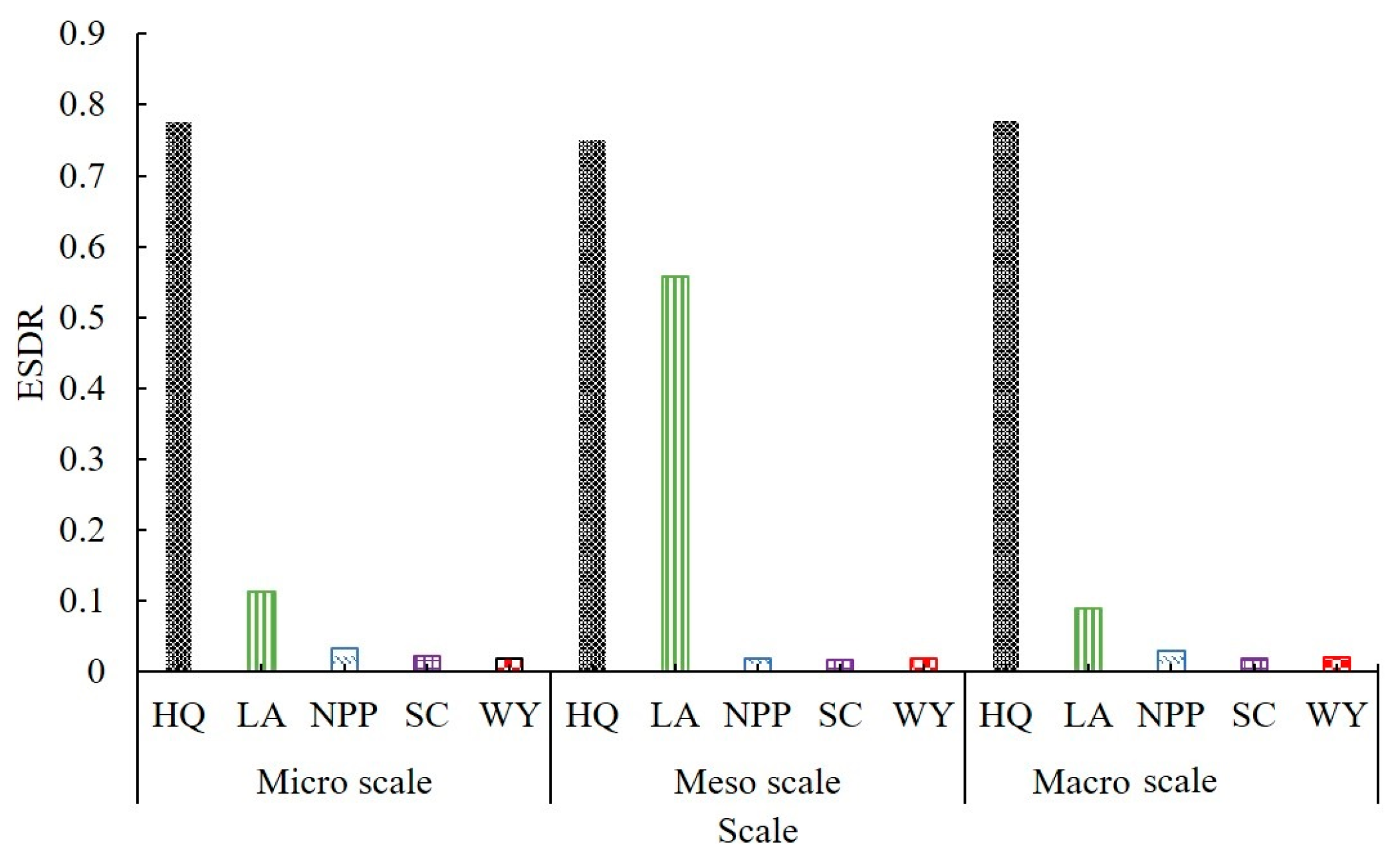
3.2.2. Ratio of Supply and Demand for Ecosystem Services

This study utilized the correlation analysis method (Figure 10) to assess the correlation coefficients between ecosystem service supplies at different scales. The results demonstrated that the tradeoffs and synergistic relationships between ecosystem service supply and demand varied depending on the scale. Notably, the supply–demand relationships for all five ecosystem services were significantly correlated across all three scales. Based on the distribution of the mean ESDR values of the five ecosystem services, it can be observed that the mean ESDR values of HQ, CS, NPP, and WY were inconsistent across the three scales. However, the mean ESDR value of LA was significantly higher than that of micro and macroscales at the mesoscale, suggesting that LA has a surplus at the mesoscale. The internal variation in the five ecosystem services at the three scales showed relatively small fluctuations, indicating a relatively smooth supply and demand status in the region. Therefore, there is unlikely to be a large-scale problem of differences between supply and demand.

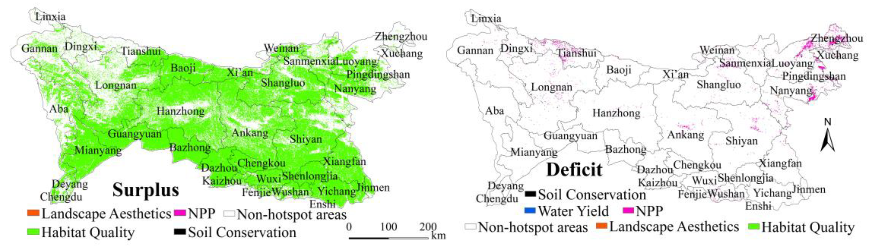
3.3. Identification of Hotspots

Based on the spatial supply–demand and tradeoff analyses, identifying hotspot areas offers valuable insights into the strengths and weaknesses of the capacity to supply and demand services in various regions. It is important to note that while the same ecosystem can provide multiple services, such as woodlands offering both water retention value quantity and NPP value quantity, the ability to provide these services and meet regional demand can vary in magnitude. This variation is reflected in the ratio of service supply and demand per unit area, which can be either large or small. This study identified hotspots for five ecosystem services in the Qinling–Daba Mountain area based on the supply–demand ratios. The ecosystem services considered were NPP, water yield, soil conservation, habitat quality, and landscape aesthetics [47]. The term ‘hotspots of 0, 1, 2, 3, 4, and 5 services’ refers to areas that can provide 0, 1, 2, 3, 4, and 5 services, respectively, exceeding the regional average. The supply–demand ratios of the five ecosystem services were divided to determine the surplus and deficit areas. The dominant ecosystem service for each hotspot mapping was identified by the maximum and minimum values of each raster.
According to the percentage analysis of the total land area in the Qinling–Daba Mountains, the hot spot areas with supply and demand ratios of the five ecosystem services below the average from 2000 to 2020 accounted for 13.14% of the total area. The proportion of hotspots with supply and demand ratios of one, two, and three ecosystem services higher than the annual average was 16.23%, 20.11%, and 23.87%, respectively. The proportion of hotspots with supply and demand ratios of the five ecosystem services that were higher than the annual average was only 7.38%. Overall, all the service supply and demand hotspot areas only accounted for 7.38% of the total area. Croplands, grasslands, and forestlands were the main land use types in these multiple ecosystem service supply and demand hotspot areas (Figure 11). The supply–demand ratios of multiple services in the southwestern and southeastern parts of the Qinling–Daba Mountains from 2000 to 2020 were generally high, indicating they can meet the demand for five ecosystem services. However, the central and northeastern parts of the region struggled to meet the demand for ecosystem services and cannot provide high-quality ecosystem service supply effectively. This is mainly due to the significant amount of arable land, rapid economic and urbanization growth, and population concentration in these areas. By using the multiple ecosystem service supply and demand hotspot map, we can clearly identify the impact of ecosystem service supply and demand in the Qinling–Daba Mountain area and determine which areas have a high demand for ecosystem services.
The dominant ESDR hotspots primarily indicate the overall situation of regional ecosystem service supply and demand. In this study, the hotspot map was divided into two categories: ecosystem service surplus hotspots and deficit hotspots (Figure 12). The spatial distribution patterns of these two categories showed clear consistencies. Among them, the ecosystem service surplus hotspot revealed that 90% of the region was covered by habitat quality services, indicating that the regional supply of ecosystem services exceeded the demand by a significant margin, resulting in a large surplus. Consequently, the entire region was predominantly characterized by habitat quality services (Figure 13). The deficit analysis of ecosystem services revealed that 1.9% of the region experienced significant deprivation of NPP. This deprivation was concentrated in areas such as Yichuan County, Dengfeng City, Xinmi City, and Gangu County. Additionally, the deprivation of soil conservation services was sporadically distributed in the Wudu District and Minxian County of Gansu Province. The main cause of this deprivation was the limited supply of regional carbon sequestration services. Furthermore, there was a surge in demand for carbon sequestration services from human activities and economic development, exacerbating the supply–demand gap for carbon sequestration in the region.

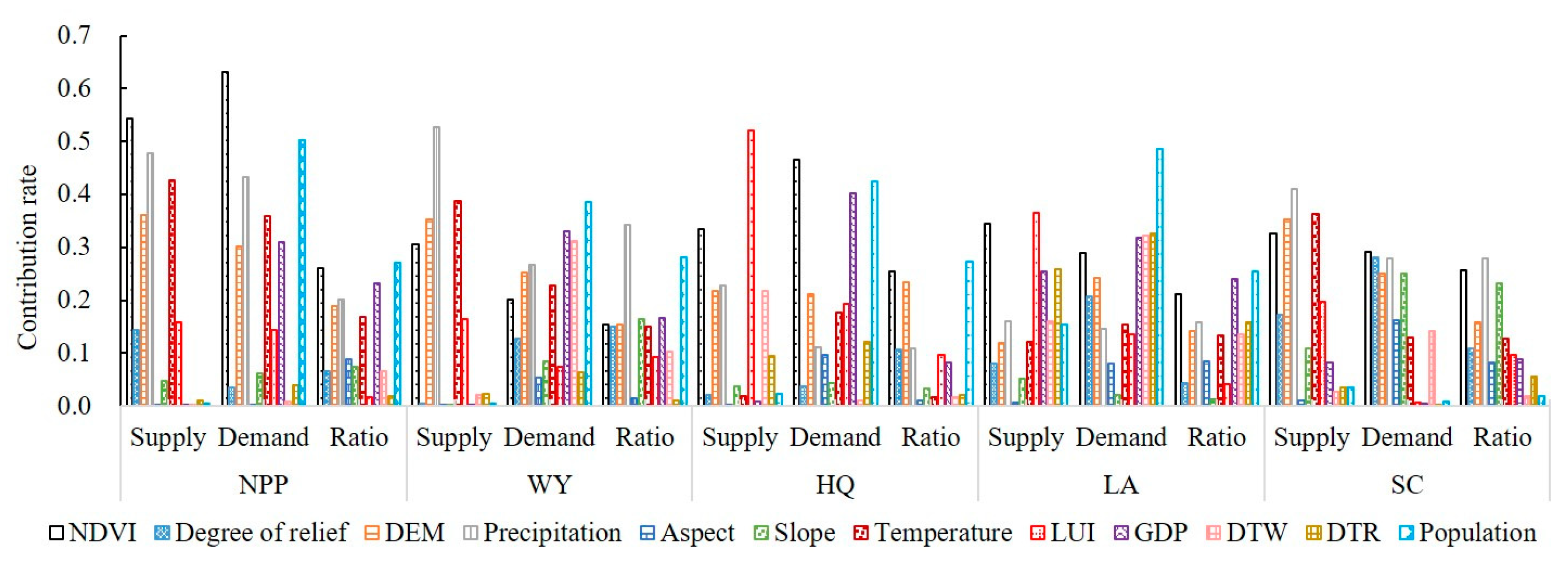
3.4. Analysis of Driving Factors

The spatiotemporal changes in ecosystem services are influenced by external drivers, which in turn affect the structure and process of ecosystem services. Understanding the factors that influence ecosystem services can effectively explain these changes. In this study, we used geographical detectors to simulate and analyze the causes of spatiotemporal changes in ecosystem services in the Qinling–Daba Mountain area. We also examined tradeoffs and synergistic relationships and quantitatively assessed the impacts of driving factors on ecosystem services. In this study, factors such as precipitation, temperature, digital elevation model (DEM), degree of relief, aspect, slope, distance from water (DTW), distance from road (DTR), population density (POP), gross national product (GDP), land use intensity (LUI), and ecological factors such as the normalized difference vegetation index (NDVI) were selected [48,49,50,51]. The drivers were modeled using the natural discontinuity method in ArcGIS software and then reclassified to obtain the base data for the study drivers, as required by the geographical detectors.
The results obtained from the factor detector reveal the individual contributions of each driver to the spatial distribution of ecosystem services (Figure 14). There are variations in the extent of influence that different drivers have on ecosystem services. In terms of carbon-sequestration services, the NDVI factor (0.544) and precipitation (0.477) were found to have the highest contribution rates. For water yield services, the contribution rates in descending order were precipitation (0.527), air temperature (0.387), DEM (0.352), and the NDVI (0.305). This indicates that precipitation and air temperature are the dominant factors influencing the spatial distribution of water yield services. The spatial distribution of water yield services in different regions is influenced by various factors. These include precipitation, temperature, land use intensity (0.522), and the NDVI (0.335). Among these factors, land use intensity and the NDVI have a significant impact on water yield services. Additionally, the contribution rate of landscape aesthetic services is influenced by land use intensity (0.366), the NDVI (0.345), population density, and GDP. Precipitation (0.411), temperature (0.363), and the NDVI (0.326) play a more prominent role in regional soil conservation services. Natural factors, particularly surface vegetation, have a positive effect on regional soil conservation. In the demand for ecosystem services, population density and GDP had a more significant effect on NPP, water yield, habitat quality, and landscape aesthetics services, respectively. Additionally, DTR and DTW contributed 0.3228 and 0.3268 to landscape aesthetics services, respectively. The factors that had a greater effect on the ratio of ecosystem supply to demand were precipitation, the NDVI, and population density. For example, NPP, HQ, and LA contributed to population density, with contributions of 0.27, 0.2726, and 0.2541, respectively. Moreover, soil conservation and water yield services were influenced more by the NDVI (0.256) and precipitation (0.3426), respectively.
The drivers of ecosystem service tradeoffs in the Qinling–Daba Mountains varied significantly (Table 3). Natural factors emerged as the primary drivers of changes in ecosystem service tradeoffs. Among these factors, the NDVI (0.526) had the most significant impact on SC and NPP tradeoffs, while slope direction (0.010) was identified as the weakest driver. Precipitation (0.498) had the most significant effect on tradeoffs related to WY and NPP, WY and HQ, WY and LA, and WY and SC, while social factors had lesser effects, all below 0.1. NDVI had the greatest influence on HQ and NPP, LA and NPP, SC and NPP, SC and HQ, and SC and LA tradeoffs, with contributions of 0.417, 0.46, 0.526, 0.401, and 0.548, respectively. DTR had a more pronounced effect on tradeoffs related to landscape aesthetic services, such as LA and NPP (0.24), LA and HQ (0.259), and SC and LA (0.174). Additionally, DEM played a crucial role in the tradeoff relationship between ecosystem services, specifically in LA and NPP (0.423), LA and HQ (0.428), SC and NPP (0.393), and HQ and NPP (0.386).

4. Discussion

4.1. Scale Effects on the Distribution of ES Supply and Demand

The interaction between ecosystem services is influenced by scale [52,53,54,55]. Understanding the supply–demand relationship of multiple ecosystem services at different spatiotemporal scales can help optimize ecosystem service management and achieve a beneficial outcome for both human society and the ecosystem [56,57]. This study analyzed the heterogeneity of the supply and demand patterns of ecosystem services at multiple scales and analyzed the influence of scale on the supply and demand of ecosystem services and the changes in the inter-relationships between supply and demand. On the one hand, it was found that the macroscale supply and demand patterns involve macro-control of the meso- and microscale patterns, while the microscale pattern is a more detailed reflection of the macroscale, and the spatial pattern of ecosystem services is characterized by better consistency. On the other hand, the differences in ecosystem services supply and demand patterns at the macroscale level objectively reflect the differences in geographic subdivisions, while the mesoscale level refines the internal differences in geographic subdivisions. The microscale level contributes to the detailed characterization of spatial and temporal changes in the supply and demand of ecosystem services within the region. At different scales (macro-, meso-, and microscale), ecosystem management tasks vary based on economic, ecological, and social factors. Macroscale ecosystem management involves identifying key ecological issues and determining protection strategies based on the characteristics and environmental conditions of larger ecosystems. Mesoscale ecosystem management is a fundamental component of macro-ecosystem management. It serves to further divide the macro pattern and offers guidance on the protection of ecological land and arable land, such as forests and grasslands. Moreover, it formulates key directions and strategies for ecological environment protection. Additionally, microscale ecosystem management necessitates clearer management plans and indicator requirements.
The findings of this study regarding the supply, demand, supply–demand ratio, and tradeoff synergy of ecosystem services can be categorized into three distinct scale differences. Firstly, the types of ecosystem service provisions and spatial layouts vary across different spatial scales. This study found that the supply of five types of ecosystem services varied across different spatial scales. Managers of localized areas need to consider the spatial extent of the role of ecosystem services. Additionally, the types of demand and spatial layout of ecosystem services differ at different spatial scales. Indicators such as the population density and GDP influenced the magnitude of demand in this study. This often leads to a spatial mismatch between supply and demand, which worsens ecosystem service conflicts. Therefore, managers need to consider the spatial differences in the importance attached by humans to different types of ecosystem services [56,58,59]. Soil retention primarily benefits the regional scale, while landscape aesthetics and habitat quality maintenance have a broader impact on the macroscale level. This distinction in the importance of different types of service products is influenced by stakeholders at different spatial scales and can lead to tradeoffs in management strategies. Additionally, transferring service products across space can create competition and tradeoffs between regions. For example, the competition for drinking water irrigation between upstream and downstream regions of rivers can lead to negative consequences such as river degradation, compromised river storage and flood control, reduced water purification services, and a weakening of various ecosystem services [56].

4.2. Drivers of Ecosystem Services

Understanding the relationship between ecosystem services and exploring their drivers is crucial for effective ecosystem management in mountainous areas [49]. This study utilized geographical detectors to identify the dominant drivers of ecosystem services. The northwestern plateau area exhibited high values of tradeoffs for water yield and soil conservation (WY and SC). This region has undulating terrain, and topography played a significant role in the tradeoff relationship between WY and SC. Moreover, higher slopes have a greater impact on the tradeoffs between WY and SC [60]. It is important to note that an increase in water yield (WY) can potentially lead to soil erosion, thereby increasing the tradeoffs between WY and SC [61]. The distribution of high WY and NPP tradeoffs was mainly observed in the western part of the Funiu and Qinling Mountain ranges, with a general decrease from north to south. This trend can be attributed to the increase in vegetation cover and improvement in habitat quality from north to south. However, this also led to strengthened evapotranspiration and reduced ground water storage capacity. In cases of a certain amount of precipitation, higher evapotranspiration resulted in a lower WY [62].
Wang et al. (2017) demonstrated that areas with high NPP typically experience abundant precipitation, which in turn increases soil erosion and leads to a decrease in SC. Therefore, the tradeoff between SC and NPP exhibits a decreasing trend from south to north, with high tradeoff values primarily located in the central subtropical climate zone [63]. Previous studies have demonstrated that temperature, precipitation, and NDVI factors play a significant role in tradeoffs in the subtropical region [64]. In the northwestern region, tradeoffs are mainly influenced by elevation due to its high frequency of terrain undulation. Conversely, in the central region, the tradeoffs between WY and SC, WY and NPP, and SC and NPP are primarily impacted by precipitation and vegetation factors. The dominant vegetation type in this region is deciduous broadleaved forests with a relatively high forest cover, thus making precipitation and NDVI factors the major contributors to tradeoffs [65]. The plateau climate zone exhibits a complex and varied topography, with significant vertical changes in topography and terrain. Consequently, the tradeoffs are mostly influenced by precipitation and NDVI factors [65]. The topography and landscape of the plateau climate zone are highly varied and complex, with significant elevation changes. As a result, the slope plays a major role in the tradeoff relationship between water yield (WY) and soil conservation (SC) [66]. In a study by Wang et al. (2022), it was found that climatic and topographic factors had the greatest influence on the tradeoff relationships between WY and net primary productivity (NPP) and between SC and NPP. On the other hand, social factors did not have a significant impact on these tradeoff relationships [49].
It has been observed that the response of climate to the supply and demand ratio of various ecosystem services varies. For instance, based on the contribution value, it is evident that the supply and demand ratio of soil conservation services and water yield services strongly correlate with precipitation. Upon further analysis, we found that soil conservation and water yield services, which are highly responsive to climate, exhibit significant changes with abundant precipitation. These changes include lush vegetation growth, reduced erosive power of rainwater on the soil, and improved soil conservation capacity. Additionally, increased precipitation also affects water yield. Moreover, topography and slope impact the supply and demand of ecosystem services. Sun et al. (2020) conducted a redundancy analysis study and found a correlation between topography and ecosystem services [67]. Furthermore, our research indicates that different ecosystem service supply/demand ratios respond differently to topography. This study revealed that the impact of the digital elevation model (DEM) on the supply–demand ratio of water yield services was more significant regarding contribution values. This could be attributed to the fact that topography affects precipitation and air temperature, thereby influencing water yield. However, it is challenging for residents in high mountain areas to sustain themselves economically due to limited human gathering places and lower demand for ecosystem services. Moreover, intensifying human activities exacerbates the conflict between ecosystems and economic development. Wang et al. (2021) discovered that the increase in water demand resulting from population growth will surpass the impact of climate warming. Consequently, both the Indus and Yarlung Zangbo River basins are projected to face water scarcity by the end of the century, leading to severe water stress for many people [68]. Therefore, it is crucial to actively pursue measures that ensure the capacity to supply ecosystem services, regulate human demand on ecosystems, and safeguard sustainable regional development and ecological security.

4.3. Optimization of Ecological Space Based on Supply and Demand of Ecosystem Services

With the increase in global population and rapid socio-economic development, the demand for services such as food, water, and carbon sequestration is expected to increase dramatically. This, in turn, will have a significant impact on the status of ecosystem services [69]. Conducting research on the supply and demand of ecosystem services at multiple scales can assist decision-makers in developing management approaches that align with societal decisions [70]. Generally, ecosystem management studies conducted at larger scales should have a lower spatial resolution and cover larger study areas. In addition, smaller scales require a finer scale of analysis to study the spatial heterogeneity of ecosystem service supply and demand. It is important to note that ecosystem service supply and demand are influenced by natural and ecological processes at different spatial and temporal scales, each with its own scale effects [71,72]. At both macro- and mesoscales, the supply of carbon-sequestration services in the Qinling Mountains is more than sufficient to meet the population’s demand in southern Shaanxi. In fact, the supply greatly exceeds the demand. However, at the provincial scale, the supply and demand of carbon-sequestration services are relatively balanced. Through a hotspot analysis (Figure 10), it was observed that the same ecosystem can offer various services. For instance, woodlands can provide both water yield and carbon storage functions. However, the extent to which these two ecosystem services are provided varies, resulting in different service sizes per unit of area [73]. To ensure the regional ecosystem service supply capacity and to balance the supply and demand of multiple ecosystem services at the macro- and mesoscale levels, policy recommendations can be implemented based on this study. For instance, regions experiencing rapid economic development, population agglomeration, and high ecosystem service demand capacity, such as Hanzhong City and Zhengzhou City, often face a regional supply mismatch. In such cases, it is essential to suggest measures like implementing ecological and environmental protection initiatives, adjusting regional water prices, and promoting water-saving agriculture. These measures can enhance the regional supply capacity and balance regional ecosystem service supply and demand.
When analyzing the surplus of the supply and demand for ecosystem services, it is evident that the Qinling–Daba Mountain area has a more pronounced surplus in habitat quality than other ecosystem services. This surplus highlights the area’s rich biodiversity, making it capable of effectively meeting regional human needs. However, the supply and demand of other ecosystem services in the area are relatively small and insufficient to meet long-term human needs. In order to address the mismatch between the supply and demand of ecosystem services caused by urbanization, it is necessary to implement ecological protection measures and policy recommendations at different scales. For example, in arid and semi-arid areas, it is necessary to strengthen the protection of grassland resources, strictly restrict overgrazing, strictly prohibit grassland cultivation, control human activity intensity, prevent land and vegetation degradation, and limit the scale of land cultivation, such as in the northwest region of China [74,75]. In areas with severe soil erosion, we should actively develop ecological agriculture, improve water sources and water-saving irrigation projects, reduce soil erosion, improve agricultural production conditions, and accelerate desertification land management, such as in the Loess Plateau region of China. The watershed should accelerate the protection and restoration of ecosystems along the river, build green ecological corridors along the river, protect important wetlands along the river and other major ecological restoration projects, enhance water source conservation and soil and water conservation functions, and rely on the rich biodiversity resources to develop characteristic industries such as ecological agriculture and ecotourism, as seen in the Yangtze River Basin in China [76].

4.4. Uncertainties and Limitations

This study provides a valuable assessment of the supply and demand for ecosystem services at different scales, along with an analysis of the driving mechanisms. It offers important clues and suggestions for better coordination between the supply of ecosystem services and the demands of society. However, there are limitations in this study that should be addressed in future research. In macro- and mesoscale studies, the lack of data availability is restricted the use of indicators such as population and economic density to characterize the demand for ecosystem services. Additionally, factors like ability, gender, wealth, and residence were not considered when assessing the demand, which may not fully capture the nuanced expression of demand in each region [19,77]. Furthermore, the process of spatializing economic data at the microscale may have compromised the reliability of the results at that level [78]. In order to improve the accuracy of this analysis, future studies should consider using questionnaires or sampling methods on a smaller scale. This will allow for analyzing a larger number of case studies and field observation data from different regions. Additionally, the selection of the driving factors in this study was not comprehensive enough. For example, only precipitation and temperature were considered as climate factors. In future studies, it is recommended to include more factors to analyze the ecosystem service driving mechanisms.

5. Conclusions

In this study, we analyzed the spatial patterns of supply and demand for five ecosystem services in the Qinling–Daba Mountain region from 2000 to 2020. We explored the relationships among these ecosystem services, as well as the effects of supply and demand, and analyzed the driving mechanisms behind their changes. The findings revealed that: (1) the scale has a certain influence on the spatial pattern of ecosystem services. The supply and demand of ecosystem services show similarities at micro- and mesoscales, but the gap becomes more apparent between the meso- and macroscales. (2) The relationship between the supply and demand of ecosystem services varies at different scales. The supply relationship is the most significant at the mesoscale, while the demand relationship is most significant at the macroscale. Additionally, there is a shift from a synergistic relationship at the microscale to a trade-off relationship at the macroscale. (3) The statistical indicators of the ESDR values for the five ecosystem services showed significant variations across different scales. The distribution of ESDR values for LA exhibited considerable variability at different scales, while the ESDR for NPP, WY, and SC remained relatively stable across the three scales. (4) Precipitation and NDVI were identified as the primary factors influencing the supply of ecosystem services. On the other hand, population density and GDP were found to have a major impact on the demand and supply/demand ratio of these services. Furthermore, natural factors were recognized as the primary drivers of changes in trade-offs among ecosystem services.

Author Contributions

Conceptualization, Y.Y.; methodology, Y.Y. and L.H.; software, Y.W.; validation, J.L. and S.Z.; formal analysis, Y.Y.; resources, L.H.; data curation, S.Z.; writing—original draft preparation, Y.Y.; writing—review and editing, Y.Y. and Y.W.; visualization, J.L.; supervision, J.L.; funding acquisition, J.L. and L.H. All authors have read and agreed to the published version of the manuscript.

Funding

This research was financially supported by the National Natural Science Foundation of China: No. 42071285; the National Science and Technology Fundamental Resources Investigation “Comprehensive Scientific Investigation of China’s North-South Transitional Zone”, “Basic Geographic Elements and Major Resources Investigation and Mapping: 2017FY100905; the Scientific Research Initiation Project for Doctor Talents No. QD2021092; the major special projects of the National High-Resolution Earth Observation System (92-Y50G35-9001-22/23); and the 2023 Henan Province key research and development and promotion of special projects (scientific and technological research). No. 232102320267.

Data Availability Statement

The land use, land resources, and population flow data in this study are publicly accessible, and the URLs are contained within this article.

Conflicts of Interest

The authors declare no conflict of interest.

Appendix A

A.1. Supply and Demand Assessment of ESs

A.1.1. Water Yield

In this paper, the InVEST model was utilized to quantify the supply of water yield services in the Qinling–Daba Mountain region. The demand for water yield services was determined by considering the amount of ecosystem services (ESs) consumed by human beings, specifically water consumption [32,33]. To obtain the data for domestic water, industrial water, farmland irrigation water, and the resident population from 2000 to 2020, the water resources bulletins of five provinces and one city were referenced. Additionally, the water consumption per capita during the same period was determined. By incorporating the population density data in grid format, a demand map for water yield services was generated. The formula used is as follows:
(1) Supply:
Y ( x ) = ( 1 AET ( x ) P ( x ) ) × P ( x )
(2) Demand:
W S ( x , t ) = p o p ( x , t ) × l i + i n d ( x , t ) × m i + a g r ( x , t ) × n i
where Y(x) is the water supply of year (m3/km2), AET(x) is the actual evaporation of the year (mm), and P(x) is the annual precipitation of the year (mm). WS (x, t) represents the total water resource service demand in Qinling–Daba mountain area (m3), li is the per capita domestic water consumption (t/a) of a city, mi is the average water consumption per ten thousand yuan of industrial output value of a city (ten thousand RMB/m3), ni is the average irrigation water consumption per mu of a city (mu/m3), pop(x, t) is population density (person/km2), ind(x, t) is spatial distribution kilometer grid of the total industrial output value (ten thousand RMB/km2), and agr(x, t) denotes farmland grid unit (acreage).

A.1.2. Habitat Quality

The habitat quality in the Qinling–Daba Mountain was examined using the habitat quality module of InVEST [34], which assigns habitat quality values ranging from 0 to 1 based on different land use types. The demand for habitat quality is determined by the human population’s reliance on the habitat provided by these land types. To estimate this demand, the product of the habitat capacity and population density for each land type was calculated. The calculation formula is as follows:
(1) Supply:
Q x j = H j ( 1 ( D x j z / ( D x j z + k z ) ) )
(2) Demand:
Q d = Q ( x ) × p ( x )
Q ( x ) = Q i   / P
Q i = ( N P P i N P P m e a n + y i y m e a n ) / 2
y i = N D V I i N D V I m i n N D V I m a x N D V I m i n
where Qxj is the habitat quality of grid x in land use type j, Dxj is the habitat stress level of grid x in land use type j, and K is the scaling parameter. Qd represents the demand for habitat quality; NPPi and NPPmean represent the average net primary productivity of vegetation in grid I and the average value of net primary productivity, respectively; yi and y mean are the average vegetation coverage and vegetation coverage in grid i; NDVImax and NDVImin are the maximum and minimum values of NDVI in the study area, respectively; P is the total number of people; Q(x) is the quality of habitat required per person for pixel x; and p(x) is the population density of pixel x.

A.1.3. Landscape Aesthetics

The aesthetic appeal of scenic spots plays a crucial role in the development of tourism. In this article, we introduced the visual quality index (VQI), which incorporates five parameters: terrain, water source, green space, human impact, and accessibility [35,36]. The original VQI included a historical parameter instead of accessibility. However, in order to account for the significant impact of data availability and landscape aesthetics on tourist attraction, we opted to include accessibility as one of the parameters. This simplified the process of quantifying the five parameters in the VQI. Our study utilized DEM, distance to water, vegetation coverage, percentage of land development, and distance to major roads to quantify these five parameters. The scores of each parameter were then combined to calculate the total VQI score, which represents the relative aesthetic value of the grid unit. The calculation formula is as follows:
(1) Supply:
V Q I x t = V Q I p + V Q I b + V Q I g + V Q I h + V Q I a
where VQIxt is the total VQI score (dimensionless) of x grid, and the value range is [0, 1]. VQIp is the terrain parameter score of grid x, VQIb is the water parameter score of grid x, VQIg is the green space parameter score of grid x, VQIh is the score of the human impact parameter of grid x, and VQIa is the score of landscape accessibility parameter for grid x.
(2) Demand:
Tourism is a significant industry in the study area, and the demand for landscape aesthetics is measured by the number of tourists per unit area [36]. As there is considerable variation in the tourist density across different regions, we employed the logarithmic method to represent the local demand for aesthetic services.
D V Q I = lg ( P p o p / S )
where DVQI is the total demand score of grid x (dimensionless), Ppop is the number of visitors in the area in a year, and S is the area of the study area.

A.1.4. Soil Conservation

In this study, soil conservation was evaluated based on the provision of soil conservation services. The demand for soil conservation services was determined by considering the actual soil erosion as an indicator of the quantity of ecological services expected by human beings [37]. Since humans are responsible for managing soil erosion, the actual amount of soil erosion was considered as the demand for soil conservation services. The modified revised universal soil loss equation (RUSLE) was employed to estimate the regional soil conservation and soil erosion. The calculation formula is as follows:
(1) Supply:
A = R × K × L S × ( 1 C × P )
(2) Demand:
U S L E = R × K × L S × C × P
where A is the soil conservation capacity (t/ha), R is the precipitation erosivity factor (MJ.mm/hm2.h.a) [38], LS is the topographic factor [39,40], K is soil erodibility index (t.hm2.h/MJ.hm2.mm), C is vegetation cover management factor [41], and P is soil and water conservation factor.

A.1.5. Net Primary Productivity

Net primary productivity is a crucial regulatory service in ecosystems [42]. In this study, we employed the CASA model to evaluate the provision of carbon sequestration services in the Qinling–Daba Mountain region from 2000 to 2020. We considered the per capita carbon emissions during this period as the demand for carbon sequestration services in the Qinling–Daba Mountain area. By utilizing the total energy consumption data for the same time frame, we calculated the total carbon emissions from 2000 to 2020 by multiplying it with the carbon emission coefficient. Subsequently, we determined the per capita carbon emissions by dividing the total emissions by the permanent population in the region from 2000 to 2020 [43,44]. Finally, we combined the grid population density data with the obtained results to generate a spatial distribution map of the demand for carbon fixation services. The formula used for these calculations is as follows:
(1) Supply:
N P P ( x , t ) = A P A R ( x , t ) × ε ( x , t )
(2) Demand:
C e = x = 1 X   p ( x ) × g ( x )
C e = i = 1 3 E j × C E F j × 12 44
φ = C e P × G x G y
where APAR (x,t) (MJ/m2) is the photosynthetic effective radiation absorbed by a specific pixel in the middle of the month, ε (x,t) (g.C.MJ−1) is a factor that indicates the efficiency of converting light energy into organic compounds in a particular grid, and NPP (x,t) (t/km2) is the NPP of pixel x at time t. Ce represents the carbon emissions from human social and economic activities, which serves as a carbon source; p(x) is the spatial population density of pixel x, g(x) is the per capita carbon emission of pixel x; and x is the total number of pixels in the study area. Ej refers to the energy consumption of different energy sources, such as coal, oil, and natural gas. In this study, coal, oil, and natural gas were selected based on the main energy types mentioned in the statistical yearbook of the five provinces and one city included in the Qinling–Daba Mountain region. P represents the total population of the five provinces and one city in the Qinling–Daba Mountain region, while Gx and Gy represent the per capita GDP of the Qinling–Daba Mountain region and the five provinces and one city, respectively.

References

  1. Burkhard, B.; Kroll, F.; Nedkov, S.; Müller, F. Mapping ecosystem service supply, demand and budgets. Ecol. Indic. 2012, 21, 12–29. [Google Scholar] [CrossRef]
  2. Ma, L.; Liu, H.; Peng, J.; Wu, J.-S. A review of ecosystem services supply and demand. Acta Geogr. Sin. 2017, 72, 1277–1289. [Google Scholar] [CrossRef]
  3. Wang, J.; Zhai, T.-L.; Lin, Y.-F.; Kong, X.-S.; He, T. Spatial imbalance and changes in supply and demand of ecosystem services in China. Sci. Total Environ. 2019, 657, 781–791. [Google Scholar] [CrossRef] [PubMed]
  4. Zhang, L.-W.; Fu, B.-J. The progress in ecosystem services mapping: A review. Acta Ecol. Sin. 2014, 35, 316–325. [Google Scholar] [CrossRef]
  5. Costanza, R.; de Groot, R.; Sutton, P.; van der Ploeg, S.; Anderson, S.-J.; Kubiszewski, I.; Farber, S.; Turner, R.-K. Changes in the global value of ecosystem services. Glob. Environ. Chang. 2014, 26, 152–158. [Google Scholar] [CrossRef]
  6. Jiang, B.; Bai, Y.; Chen, J.-Y.; Alatalo, J.-M.; Xu, X.-B.; Liu, G.; Wang, Q. Land management to reconcile ecosystem services supply and demand mismatches-A case study in Shanghai municipality, China. Land Degrad. Dev. 2020, 31, 2684–2699. [Google Scholar] [CrossRef]
  7. Owuor, M.-A.; Icely, J.; Newton, A.; Nyunja, J.; Otieno, P.; Tuda, A.-O.; Oduor, N. Mapping of ecosystem services flow in Mida Creek, Kenya. Ocean. Coast. Manag. 2017, 140, 11–21. [Google Scholar] [CrossRef]
  8. De Groot, R.-S.; Wilson, M.-A.; Boumans, R.-M.-J. A typology for the classification, description and valuation of ecosystem functions, goods and services. Ecol. Econ. 2002, 41, 393–408. [Google Scholar] [CrossRef]
  9. Liu, Y.; Bi, J.; Lv, J.-S.; Ma, Z.-W.; Wang, C. Spatial multi-scale relationships of ecosystem services: A case study using a geostatistical methodology. Sci. Rep. 2017, 7, 9486. [Google Scholar] [CrossRef]
  10. Geijzendorffer, I.-R.; Martín-López, B.; Roche, P.-K. Improving the identification of mismatches in ecosystem services assessments. Ecol. Indic. 2015, 52, 320–331. [Google Scholar] [CrossRef]
  11. Jaligot, R.; Chenal, J.; Bosch, M. Assessing spatial temporal patterns of ecosystem services in Switzerland. Landsc. Ecol. 2019, 34, 1379–1394. [Google Scholar] [CrossRef]
  12. Zhang, G.-S.; Zheng, D.; Xie, L.; Zhang, X.; Wu, H.-J.; Li, S. Mapping changes in the value of ecosystem services in the Yangtze River Middle Reaches Megalopolis, China. Ecosyst. Serv. 2021, 48, 101252. [Google Scholar] [CrossRef]
  13. Turner, K.-G.; Odgaard, M.-V.; Bocher, P.-K.; Dalgaard, T.; Svenning, J.-C. Bundling ecosystem services in Denmark: Trade-offs and synergies in a cultural landscape. Landsc. Urban Plan. 2014, 125, 89–104. [Google Scholar] [CrossRef]
  14. Zwierzchowska, I.; Hof, A.; Iojă, I.-C.; Mueller, C.; Poniży, L.; Breuste, J.; Mizgajski, A. Multi-scale assessment of cultural ecosystem services of parks in Central European cities. Urban For. Urban Green. 2018, 30, 84–97. [Google Scholar] [CrossRef]
  15. Ciftcioglu, G.-C. The social valuation of agro-ecosystem services at different scales: A case study from Kyrenia (Girne) Region of Northern Cyprus. Environ. Dev. 2021, 39, 100645. [Google Scholar] [CrossRef]
  16. Xu, S.-N.; Liu, Y.-F.; Wang, X.; Zhang, G.-X. Scale effect on spatial patterns of ecosystem services and associations among them in semi-arid area: A case study in Ningxia Hui Autonomous Region, China. Sci. Total Environ. 2017, 598, 297–306. [Google Scholar] [CrossRef]
  17. Raudsepp-Hearne, C.; Peterson, G.-D. Scale and ecosystem services: How do observation, management, and analysis shift with scale- lessons from Québec. Ecol. Soc. 2016, 21, 16. [Google Scholar] [CrossRef]
  18. Roces-Díaz, J.-V.; Vayreda, J.; Banqué-Casanovas, M.; Díaz-Varela, E.; Bonet, J.-A.; Brotons, L.; de-Miguel, S.; Herrando, S.; Martínez-Vilalta, J. The spatial level of analysis affects the patterns of forest ecosystem services supply and their relationships. Sci. Total Environ. 2018, 626, 1270. [Google Scholar] [CrossRef]
  19. Wei, H.-J.; Fan, W.-G.; Wang, X.-C.; Lu, N.-C.; Dong, X.-B.; Zhao, Y.-N.; Ya, X.-J.; Zhao, Y.-F. Integrating supply and social demand in ecosystem services assessment: A review. Ecosyst. Serv. 2017, 25, 15–27. [Google Scholar] [CrossRef]
  20. Wu, X.; Liu, S.-L.; Zhao, S.; Hou, X.-Y.; Xu, J.-W.; Dong, S.-K.; Liu, G.-H. Quantification and driving force analysis of ecosystem services supply, demand and balance in China. Sci. Total Environ. 2019, 652, 1375–1386. [Google Scholar] [CrossRef]
  21. Alamgir, M.; Turton, S.-M.; Macgregor, C.-J.; Pert, L.-P. Assessing regulating and provisioning ecosystem services in a contrasting tropical forest landscape. Ecol. Indic. 2016, 64, 319–334. [Google Scholar] [CrossRef]
  22. Serna-Chavez, H.-M.; Kissling, W.-D.; Veen, L.-E.; Swenson, N.-G.; van Bodegom, P.-M. Spatial scale dependence of factors driving climate regulation services in the Americas. Glob. Ecol. Biogeogr. 2018, 27, 828–838. [Google Scholar] [CrossRef]
  23. Ouyang, Z.-Y.; Zheng, H.-W.; Xiao, Y.; Stephen, P.; Liu, J.-G.; Xu, W.-H.; Wang, Q.; Zhang, L.; Rao, E.-M.; Jiang, L.; et al. Improvements in ecosystem services from investments in natural capital. Science 2016, 352, 1455–1459. [Google Scholar] [CrossRef]
  24. Song, W.; Deng, X.-Z. Land-use/land-cover change and ecosystem service provision in China. Sci. Total Environ. 2017, 576, 705–719. [Google Scholar] [CrossRef] [PubMed]
  25. Filho, W.-L.; Barbir, J.; Sima, M.; Kalbus, A.; Nagy, G.-J.; Paletta, A.; Villamizar, A.; Martinez, R.; Azeiteiro, U.-M.; Pereira, M.-J.; et al. Reviewing the role of ecosystems services in the sustainability of the urban environment: A multi-country analysis. J. Clean. Prod. 2020, 262, 121338. [Google Scholar] [CrossRef]
  26. Fang, L.-L.; Wang, L.-C.; Chen, W.-X.; Sun, J.; Cao, Q.; Wang, S.-Q.; Wang, L.-Z. Identifying the impacts of natural and human factors on ecosystem service in the Yangtze and Yellow River Basins. J. Clean. Prod. 2021, 314, 127995. [Google Scholar] [CrossRef]
  27. Tang, X.-J.; Chen, X.-X. Thoughts on the paths of cross-regional ecological environmental governance in Qinling-Dabashan Mountainous area. J. Southwest Pet. Univ. 2019, 21, 28–34. [Google Scholar]
  28. Liu, L.-C.; Liu, C.F.; Wang, C.; Li, P.-J. Supply and demand matching of ecosystem services in loess hilly region: A case study of Lanzhou. Acta Geogr. Sin. 2019, 74, 1921–1937. [Google Scholar]
  29. Yan, Y.; Zhu, J.-Y.; Wu, G.; Zhan, Y.-J. Review and prospective applications of demand, supply, and consumption of ecosystem services. Acta Ecol. Sin. 2017, 37, 2489–2496. [Google Scholar]
  30. Han, C.-J.; Wang, G.-G.; Yang, Y.-P. An assessment of sustainable wellbeing and coordination of mountain areas: A case study of Qinba Mountain Area in China. Ecol. Indic. 2023, 154, 110674. [Google Scholar] [CrossRef]
  31. Liu, J.-J.; Zhang, B.-P.; Yao, Y.-H.; Zhang, X.-H.; Wang, J.; Yu, F.-Q.; Li, J.-Y. Latitudinal differentiation and patterns of temperate and subtropical plants in the Qinling-Daba Mountains. J. Geogr. Sci. 2023, 33, 907–923. [Google Scholar] [CrossRef]
  32. Chen, D.-S.; Li, J.; Yang, X.-N.; Zhou, Z.-X.; Pan, Y.-Q.; Li, M.-C. Quantifying water provision service supply, demand and spatial flow for land use optimization: A case study in the YanHe watershed. Ecosyst. Serv. 2020, 43, 101117. [Google Scholar] [CrossRef]
  33. Zhang, C.; Li, J.; Zhou, Z.-X.; Sun, Y.-J. Application of ecosystem service flows model in water security assessment: A case study in Weihe River Basin, China. Ecol. Indic. 2021, 120, 106974. [Google Scholar] [CrossRef]
  34. Wang, B.Y.; Oguchi, T.; Liang, X. Evaluating future habitat quality responding to land use change under different city compaction scenarios in Southern China. Cities 2023, 140, 104410. [Google Scholar] [CrossRef]
  35. Swetnam, R.-D.; Harrison-Curran, S.-K.; Smith, G.-R. Quantifying visual landscape quality in rural Wales: A GIS-enabled method for extensive monitoring of a valued cultural ecosystem service. Ecosyst. Serv. 2017, 26, 451–464. [Google Scholar] [CrossRef]
  36. Cui, F.-Q.; Tang, H.-Q.; Zhang, Q.; Wang, B.-J.; Dai, L.-W. Integrating ecosystem services supply and demand into optimized management at different scales: A case study in Hulunbuir, China. Ecosyst. Serv. 2019, 39, 100984. [Google Scholar] [CrossRef]
  37. Rao, W.-G.; Shen, Z.-H.; Duan, X.-W. Spatiotemporal patterns and drivers of soil erosion in Yunnan, Southwest China: RULSE assessments for recent 30 years and future predictions based on CMIP6. CATENA 2023, 220, 106703. [Google Scholar] [CrossRef]
  38. Wischmeier, W.H.; Mannering, J.V. Relation of soil properties to its erodibility. Soil Sci. Soc. Am. J. 1969, 33, 131–137. [Google Scholar] [CrossRef]
  39. Wischmeier, W.-H.; Smith, D.-D. Predicting precipitation fall erosion losses-A guide to conservation planning. Agric. Handb. 1978, 537, 285–291. [Google Scholar]
  40. Mccool, D.-K.; Brown, L.-C.; Foster, G.-R.; Mutchler, C.-K. Revised Slope Steepness Factor for the Universal Soil Loss Equation. Trans. ASAE Am. Soc. Agric. Eng. 1987, 30, 1387–1396. [Google Scholar] [CrossRef]
  41. Cai, C.F.; Ding, S.W.; Shi, Z.H.; Huang, L.; Zhan, G.Y. Study of applying USLE and geographical information system IDRISI to predict soil erosion in small watershed. J. Soil Water Conserv. 2000, 14, 19–24. [Google Scholar]
  42. Potter, C.-S.; Randerson, J.-T.; Field, C.-B.; Matson, P.-A.; Vitousek, P.-M.; Mooney, H.-A.; Klooster, S. Terrestrial ecosystem production: A process model based on global satellite and surface data. Glob. Biochem. Cycle 1993, 7, 811–841. [Google Scholar] [CrossRef]
  43. Li, T.; Li, J.; Wang, Y.-Z. Carbon sequestration service flow in the Guanzhong-Tianshui economic region of China: How it flows, what drives it, and where could be optimized? Ecol. Indic. 2019, 96 Pt 1, 548–558. [Google Scholar] [CrossRef]
  44. Yu, Y.-Y.; Li, J.; Zhou, Z.-X.; Zeng, L.; Zhang, C. Estimation of the Value of Ecosystem Carbon Sequestration Services under Different Scenarios in the Central China (the Qinling-Daba Mountain Area). Sustainability 2020, 12, 337. [Google Scholar] [CrossRef]
  45. Wang, J.-F.; Xu, C.-D. Geodetector: Principle and prospective. Acta Geogr. Sin. 2017, 72, 116–134. [Google Scholar]
  46. Wang, J.-F.; Li, X.-H.; Christakos, G.; Liao, Y.-L.; Zhang, T.; Gu, X.; Zheng, X.-Y. Geographical Detectors-Based Health Risk Assessment and its Application in the Neural Tube Defects Study of the Heshun Region, China. Int. J. Geogr. Inf. Sci. 2010, 24, 107–127. [Google Scholar] [CrossRef]
  47. Wu, W.-H.; Peng, J.; Liu, Y.X.; Hu, Y.-N. Tradeoffs and synergies between ecosystem services in Ordos City. Prog. Geogr. 2017, 36, 1571–1581. [Google Scholar]
  48. Wang, X.-F.; Fu, X.-X.; Chu, B.-Y.; Li, Y.-H.; Yan, Y.; Feng, X.-M. Spatiotemporal variation of water yield and its driving factors in Qinling Mountains barrier region. J. Nat. Resour. 2021, 36, 2507–2521. [Google Scholar]
  49. Wang, X.-Z.; Wu, J.-Z.; Liu, Y.-L.; Hai, X.-Y.; Shangguan, Z.-P.; Deng, L. Driving factors of ecosystem services and their spatiotemporal change assessment based on land use types in the Loess Plateau. J. Environ. Manag. 2022, 311, 114835. [Google Scholar] [CrossRef] [PubMed]
  50. Li, J.-Y.; Geneletti, D.; Wang, H.-C. Understanding supply-demand mismatches in ecosystem services and interactive effects of drivers to support spatial planning in Tianjin metropolis, China. Sci. Total Environ. 2023, 895, 165067. [Google Scholar] [CrossRef]
  51. Shen, J.-S.; Li, S.-C.; Wang, H.; Wu, S.-Y.; Liang, Z.; Zhang, Y.-T.; Wei, F.-L.; Li, S.; Ma, L.; Wang, Y.-Y.; et al. Understanding the spatial relationships and drivers of ecosystem service supply-demand mismatches towards spatially targeted management of social-ecological system. J. Clean. Prod. 2023, 406, 136882. [Google Scholar] [CrossRef]
  52. Wang, G.-C.; Li, Z.-C. The valuation of ecosystem services based on temporal, spatial and benefit characters. Acta Ecol. Sin. 2007, 27, 4758–4765. [Google Scholar]
  53. Luo, G.-P.; Zhang, A.-J.; Yin, C.-Y.; Lu, L. Progress and prospects of multi-scale evaluation of land change. Arid. Zone Res. 2009, 26, 41–47. [Google Scholar] [CrossRef]
  54. Zhang, Y.-S.; Wu, D.-T.; Lv, X. A review on the impact of land use/land cover change on ecosystem services from a spatial scale perspective. J. Nat. Resour. 2020, 35, 1172–1189. [Google Scholar]
  55. Zhang, Y.-M.; Zhao, S.-D. Contributions and lessons of multiscale assessments. Adv. Earth Sci. 2007, 22, 851–856. [Google Scholar] [CrossRef]
  56. Rodríguez, J.-P.; Douglas, B.-T.; Bennett, E.-M.; Cumming, G.-S. Trade-offs across Space, Time, and Ecosystem Services. Ecol. Soc. 2005, 11, 709–723. [Google Scholar] [CrossRef]
  57. Seppelt, R.; Fath, B.; Burkhard, B.; Fisher, J.; Grêt-Regamey, A.; Lautenbach, S.; Pert, P.; Hotes, S.; Spangenberg, J.; Verburg, P.-H.; et al. Form follows function? Proposing a blueprint for ecosystem service assessments based on reviews and case studies. Ecol. Indic. 2012, 21, 145–154. [Google Scholar] [CrossRef]
  58. Li, P.; Jiang, L.G.; Feng, Z.-M.; Yu, X.-B. Research progression trade-offs and synergies of ecosystem services: An overview. Acta Ecol. Sin. 2012, 32, 5219–5229. [Google Scholar]
  59. Bohensky, E.-L.; Reyers, B.; Van Jaarsveld, A.-S. Future ecosystem services in a Southern African river basin: A scenario planning approach to uncertainty. Conserv. Biol. 2006, 20, 1051–1061. [Google Scholar] [CrossRef]
  60. Zhang, Z.-H.; Nie, T.-T.; Gao, Y.; Sun, S.-M.; Gao, J. Study on temporal and spatial characteristics of coupling coordination correlation between ecosystem services and economic-social development in the Yangtze River Economic Belt. Resour. Environ. Yangtze Basin 2022, 31, 1086–1100. [Google Scholar]
  61. Gao, M.; Xiao, Y.; Hu, Y.-F. Evaluation of water yield and soil erosion in the Three-River-Source region under different land-climate scenarios. J. Resour. Ecol. 2020, 11, 13–26. [Google Scholar]
  62. Liu, S.-C.; Shao, Q.-Q.; Niu, L.-N.; Ning, J.; Liu, G.-B.; Zhang, X.-Y.; Huang, H.-B. Changes of ecological and the characteristics of trade-offs and synergies of ecosystem services in the upper reaches of the Yangtze River. Acta Ecol. Sin. 2023, 43, 1028–1039. [Google Scholar]
  63. Wang, P.-T.; Zhang, L.-W.; Li, Y.-J.; Jiao, L.; Wang, H.; Yan, J.-P.; Lv, Y.-H.; Fu, B.-J. Spatio-temporal characteristics of the trade-off and synergy relationships among multiple ecosystem services in the Upper Reaches of Hanjiang River Basin. Acta Geogr. Sin. 2017, 72, 2064–2078. [Google Scholar]
  64. Niu, Z.-E.; He, H.-L.; Ren, X.-L.; Zhang, L.; Qin, K.-Y.; Zhao, D.; Lv, Y. Spatio-temporal characteristic of terrestrial ecosystem services and their tradeoffs and synergies in China from 2000 to 2018 based on a process model. Acta Ecol. Sin. 2023, 43, 496–509. [Google Scholar]
  65. Sannigrahi, S.; Zhang, Q.; Pilla, F.; Joshi, P.-K.; Basu, B.; Keesstra, S.; Roy, P.-S.; Wang, Y.; Sutton, P.-C.; Chakraborti, S.; et al. Responses of ecosystem services to natural and anthropogenic forcings: A spatial regression based assessment in the world’s largest mangrove ecosystem. Sci. Total Environ. 2020, 715, 137004. [Google Scholar] [CrossRef] [PubMed]
  66. Zhang, J.; Lei, G.; Qi, L.-H. Temporal and Spatial Dynamics and Scenario Simulation of Water Yield in Danjiangkou Reservoir Area. Sci. Silvae Sin. 2020, 56, 12–20. [Google Scholar]
  67. Sun, X.-Y.; Shan, R.-F.; Liu, F. Spatio-temporal quantification of patterns, trade-offs and synergies among multiple hydrological ecosystem services in different topographic basins. J. Clean. Prod. 2020, 268, 122338. [Google Scholar] [CrossRef]
  68. Wang, T.; Zhao, Y.-T.; Xu, C.-Y.; Ciais, P.; Liu, D.; Yang, H.; Piao, S.-L.; Yao, D.-T. Atmospheric dynamic constraints on Tibetan Plateau freshwater under Paris climate targets. Nat. Clim. Chang. 2021, 11, 219–225. [Google Scholar] [CrossRef]
  69. Peng, S.-M.; Zheng, X.-K.; Wang, Y.; Jiang, G.-Q. Study on water-energy-food collaborative optimization for Yellow River basin. Adv. Water Sci. 2017, 28, 681–690. [Google Scholar]
  70. García-Nieto, A.-P.; García-Llorente, M.; Iniesta-Arandia, I.; Martín-López, B. Mapping forest ecosystem services: From providing units to beneficiaries. Ecosyst. Serv. 2013, 4, 126–138. [Google Scholar] [CrossRef]
  71. Fu, B.-J.; Zhang, L.-W. Land-use change and ecosystem services: Concepts, methods and progress. Prog. Geogr. 2014, 33, 441–446. [Google Scholar]
  72. Yan, W.-T.; Huang, Y.; Zou, J. Ecosystem services integrated urban and rural land use planning: Conceptual framework and practical approach. Landsc. Archit. 2017, 1, 45–51. [Google Scholar]
  73. Hao, M.-Y.; Ren, Z.-Y.; Sun, Y.-J.; Zhao, S.-N. The dynamic analysis of trade-off and synergy of ecosystem services in the Guanzhong Basin. Geogr. Res. 2017, 36, 592–602. [Google Scholar]
  74. Ma, X.-K.; Gao, M.-H. Dynamic assessment of land ecologic safety of oasis city in arid northwest China: A case of Korla City in Xinjiang. Arid. Land Geogr. 2017, 40, 172–180. [Google Scholar]
  75. Kang, T.-T.; Li, Z.; Gao, Y. Effectiveness of ecological restoration in the mountain-oasis-desert system of northwestern arid area of China. Acta Ecol. Sin. 2019, 39, 7418–7431. [Google Scholar]
  76. Lin, Z.-Y.; Xiao, Y.; Shi, X.-W.; Rao, E.-M.; Zhang, P.; Wang, L.-Y. Assessment of the ecological importance patterns in southwest China. Acta Ecol. Sin. 2018, 38, 8667–8675. [Google Scholar]
  77. Lamarque, P.; Tappeiner, U.; Turner, C.; Steinbacher, M.; Bardgett, R.-D.; Szukics, U.; Lavorel, S.-S. Stakeholder perceptions of grassland ecosystem services in relation to knowledge on soil fertility and biodiversity. Reg. Environ. Chang. 2011, 11, 791–804. [Google Scholar] [CrossRef]
  78. Li, S.-C.; Zhang, Y.-L.; Wang, Z.-F.; Li, L.-H. Mapping human influence intensity in the Tibetan Plateau for conservation of ecological service functions. Ecosyst. Serv. 2018, 30, 276–286. [Google Scholar] [CrossRef]
Figure 1. Geographical location (a), county-level administrative boundary (at a meso scale) (b), city-level administrative boundary (at a macro scale) (c), land cover (at a micro scale) (d) and the elevation data (e) of the Qinling-Daba Mountain area.
Land 12 01744 g001
Figure 2. The methodological framework diagram of this study.
Land 12 01744 g002
Figure 3. Spatial distribution of NPP supply (in t/km2), demand (in t/km2), and ESDR at the microscale (A,D,G), mesoscale (B,E,H), and macroscale (C,F,I) levels.
Land 12 01744 g003
Figure 4. Spatial distribution of habitat quality supply, demand, and ESDR at the microscale (A,D,G), mesoscale (B,E,H), and macroscale (C,F,I) levels.
Land 12 01744 g004
Figure 5. Spatial distribution of water yield supply (in m3/km2), demand (in m3/km2), and ESDR at the microscale (A,D,G), mesoscale (B,E,H), and macroscale (C,F,I) levels.
Land 12 01744 g005
Figure 6. Spatial distribution of landscape aesthetic supply, demand, and ESDR at the microscale (A,D,G), mesoscale (B,E,H), and macroscale (C,F,I) levels.
Land 12 01744 g006
Figure 7. Spatial distribution of soil conservation supply (in t/ha), demand (in t/ha), and ESDR at the microscale (A,D,G), mesoscale (B,E,H), and macroscale (C,F,I) levels.
Land 12 01744 g007
Figure 8. Spatial distribution of ecosystem service tradeoff relationships.
Land 12 01744 g008
Figure 9. Correlation coefficients between ES indicator supply and demand pairs at different scales. (The blue color and a slash from bottom left to top right indicate a positive correlation between the two variables. On the contrary, the red and slash from top left to bottom right indicate a negative correlation. The darker the color, the higher the saturation, indicating a greater correlation between variables. The correlation size in the upper right corner is displayed by the size of the filled pie chart block, with clockwise filling indicating positive correlation and counterclockwise filling indicating negative correlation. No * means p < 0.05; ** means p < 0.01).
Land 12 01744 g009
Figure 10. A comparison of five ESDR values at three scales.
Land 12 01744 g010
Figure 11. Proportion of the area of different ESDR hotspots with different land uses.
Land 12 01744 g011
Figure 12. Distribution of hotspots of ESDR for multiple ecosystem services.
Land 12 01744 g012
Figure 13. Distribution of dominant hotspots of ESDR.
Land 12 01744 g013
Figure 14. Contribution rates of driving factors of ecosystem services.
Land 12 01744 g014
Table 1. Data sources.
Data TypeData DescriptionData Source
Basic geographic information dataAdministrative divisions, rivers, roads, etc.http://www.ngcc.cn/ngcc/
Accesses 15 May 2018
Normalized difference vegetation index, NDVI data250 m spatial resolution MOD13Q1 data, which was obtained from NASA from 2000 to 2020.https://ladsweb.modaps.eosdis.nasa.gov/
Accesses 20 January 2021
Soil data1:1 million soil data provided by Nanjing Soil Institute of the Second National Land Survey, with a spatial resolution of 1 km × 1 kmhttps://data.tpdc.ac.cn/zh-hans/
Accesses 5 April 2018
Land use dataSourced from GlobalLand30, a global geographic information public product with a spatial resolution of 30 m, from 2000 to 2020http://www.globallandcover.com/
Accesses 1 March 2021
Meteorological dataSpatially interpolated dataset of average conditions of meteorological elements in China with a spatial resolution of 1 km, from 2000 to 2020.http://www.resdc.cn/
Accesses 18 March 2021
Socio-economic data (GDP, population density, energy consumption, urban and rural water consumption, etc.)Socio-economic data, energy consumption, water utilization, and tourism numbers and revenues were almost exclusively derived from 2000 to 2020 statistical yearbooks.http://www.stats.gov.cn/
Accesses 20 December 2021
Table 2. Ecosystem services analyzed in this study.
Service CategoryES Assessment CodeUnitDescriptionSupply Quantification MethodDemand Quantification MethodReferences
ProvisioningWater yield WY m3/km2Estimated water yield per pixel based on hydrological processes such as precipitation and evapotranspirationWater yield module of Integrated Valuation of Ecosystem Services and Trade-offs (InVEST)The sum of residential water, industrial water, and farmland irrigation[32,33]
MaintenanceHabitat qualityHQProbabilityAbility of the ecosystem to provide appropriate conditions for individual and population persistence.Habitat quality module of InVESTThe product of per capita consumption and population density of habitat quality[34]
CulturalLandscape aesthetics LAScoresPotential visual appeal is controlled by inherent landscape characteristics such as topography or vegetation.Visual quality index (VQI)The logarithmic function of the number of tourists per unit area is used as the demand for landscape aesthetics[35,36]
RegulatingSoil conservationSCt/haAmount of sediment that vegetation preserved under water erosion during rainfall events.Revised universal soil loss equation (RULSE)Actual soil conservation[37,38,39,40,41]
Net primary productivityNPPt/km2Amount of carbon that is sequestered from plants and soil.Carnegie–Ames–Stanford approach (CASA)Product of per capita carbon consumption and population density[42,43,44]
Table 3. Contribution rate of driving factors to tradeoff/synergy relationships between ecosystem services.
WY and NPPHQ and NPPLA and NPPSC and NPPWY and HQWY and LASC and WYLA and HQSC and HQSC and LA
NDVI0.357 0.417 0.460 0.526 0.451 0.362 0.276 0.399 0.401 0.548
Degree of relief0.143 0.207 0.139 0.173 0.113 0.112 0.383 0.130 0.096 0.030
DEM0.309 0.386 0.423 0.393 0.307 0.101 0.232 0.428 0.294 0.281
Precipitation0.461 0.374 0.254 0.411 0.498 0.436 0.414 0.327 0.380 0.371
Aspect0.090 0.196 0.080 0.010 0.020 0.094 0.147 0.024 0.157 0.013
Slope0.034 0.098 0.095 0.029 0.034 0.160 0.346 0.067 0.144 0.116
Temperature0.242 0.250 0.351 0.363 0.377 0.218 0.379 0.417 0.260 0.239
LUI0.141 0.168 0.101 0.197 0.079 0.168 0.144 0.129 0.135 0.031
GDP0.014 0.005 0.030 0.083 0.076 0.046 0.015 0.012 0.013 0.065
DTW0.021 0.003 0.101 0.026 0.218 0.232 0.198 0.160 0.027 0.132
DTR0.023 0.010 0.240 0.034 0.094 0.233 0.017 0.259 0.006 0.174
Population0.028 0.021 0.101 0.035 0.017 0.078 0.073 0.089 0.012 0.012
Disclaimer/Publisher’s Note: The statements, opinions and data contained in all publications are solely those of the individual author(s) and contributor(s) and not of MDPI and/or the editor(s). MDPI and/or the editor(s) disclaim responsibility for any injury to people or property resulting from any ideas, methods, instructions or products referred to in the content.

