


Analysis of Land Suitability for Maize Production under Climate Change and Its Mitigation Potential through Crop Residue Management

 ,
,  , ,
, , 
Abstract
1. Introduction
2. Materials and Methods
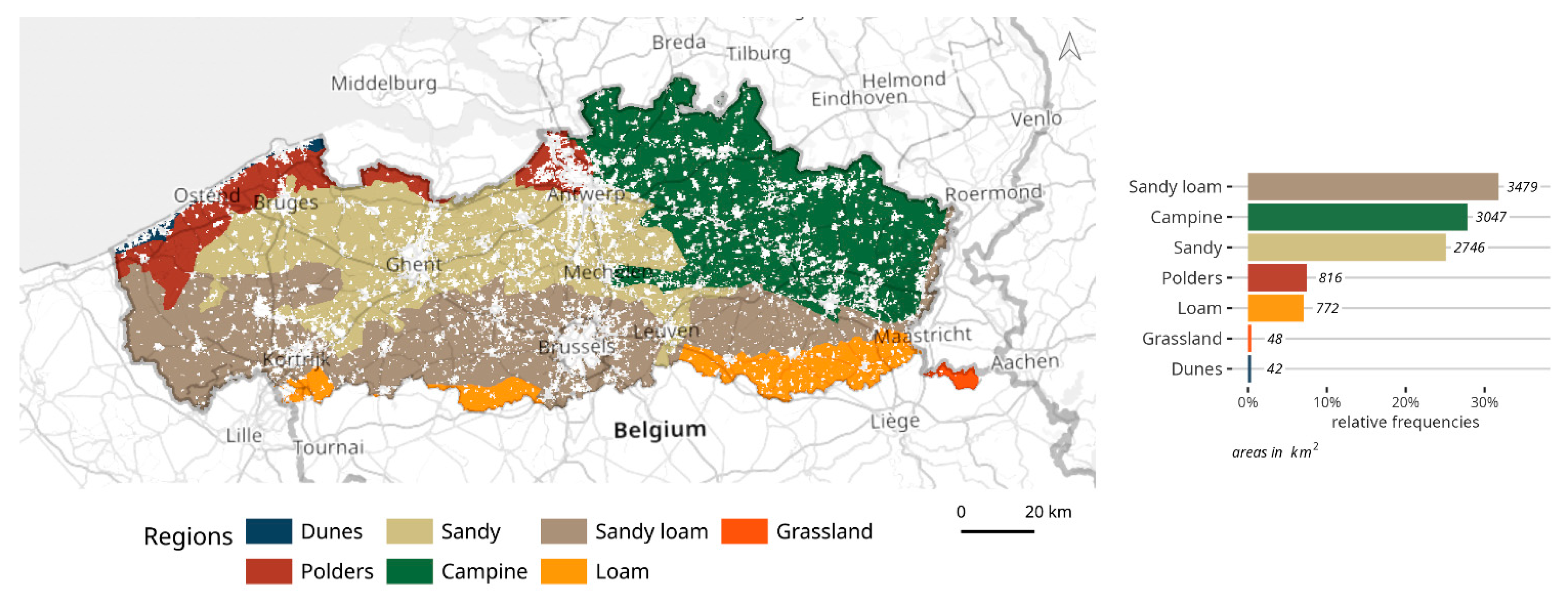
2.1. Study Area
2.2. Data Sources
2.3. LSA Application
2.3.1. Current LSA
2.3.2. Future LSA
Future LSA Computation
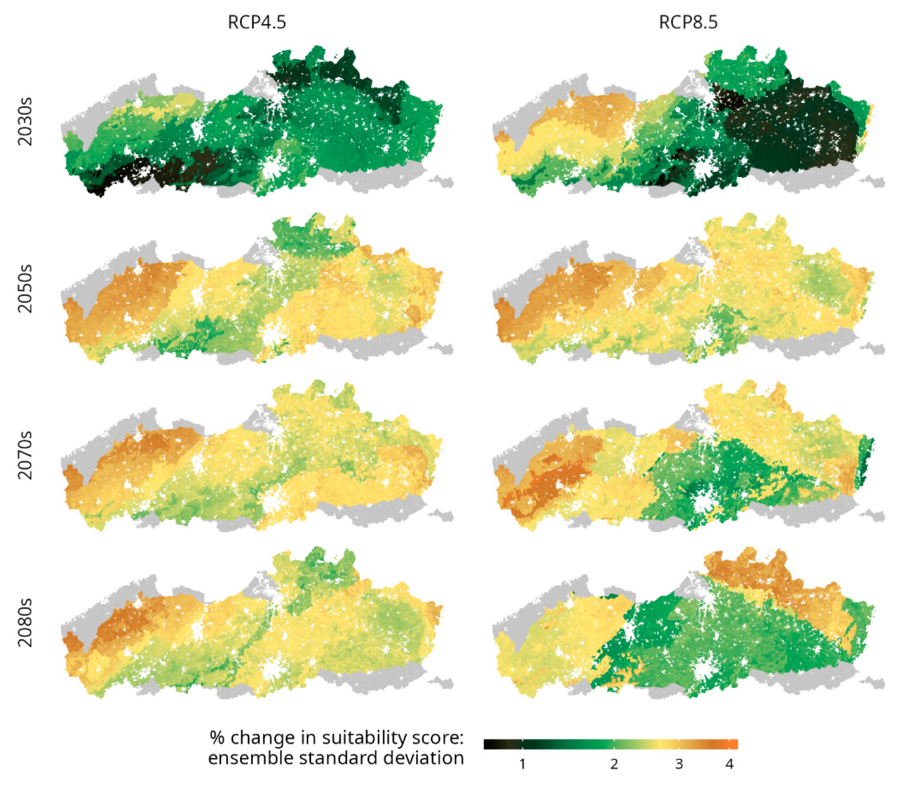
Inter-Model Spread
Future LSA under SICS
3. Results
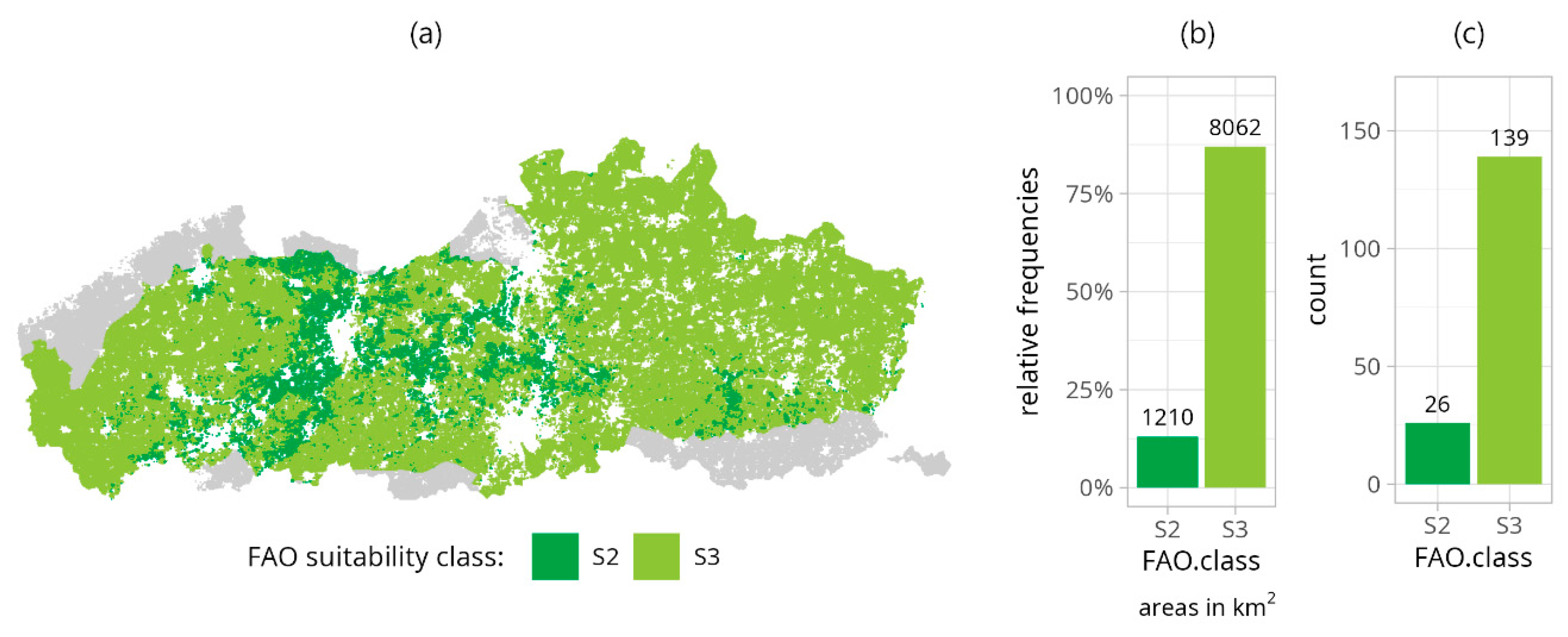
3.1. Current LSA
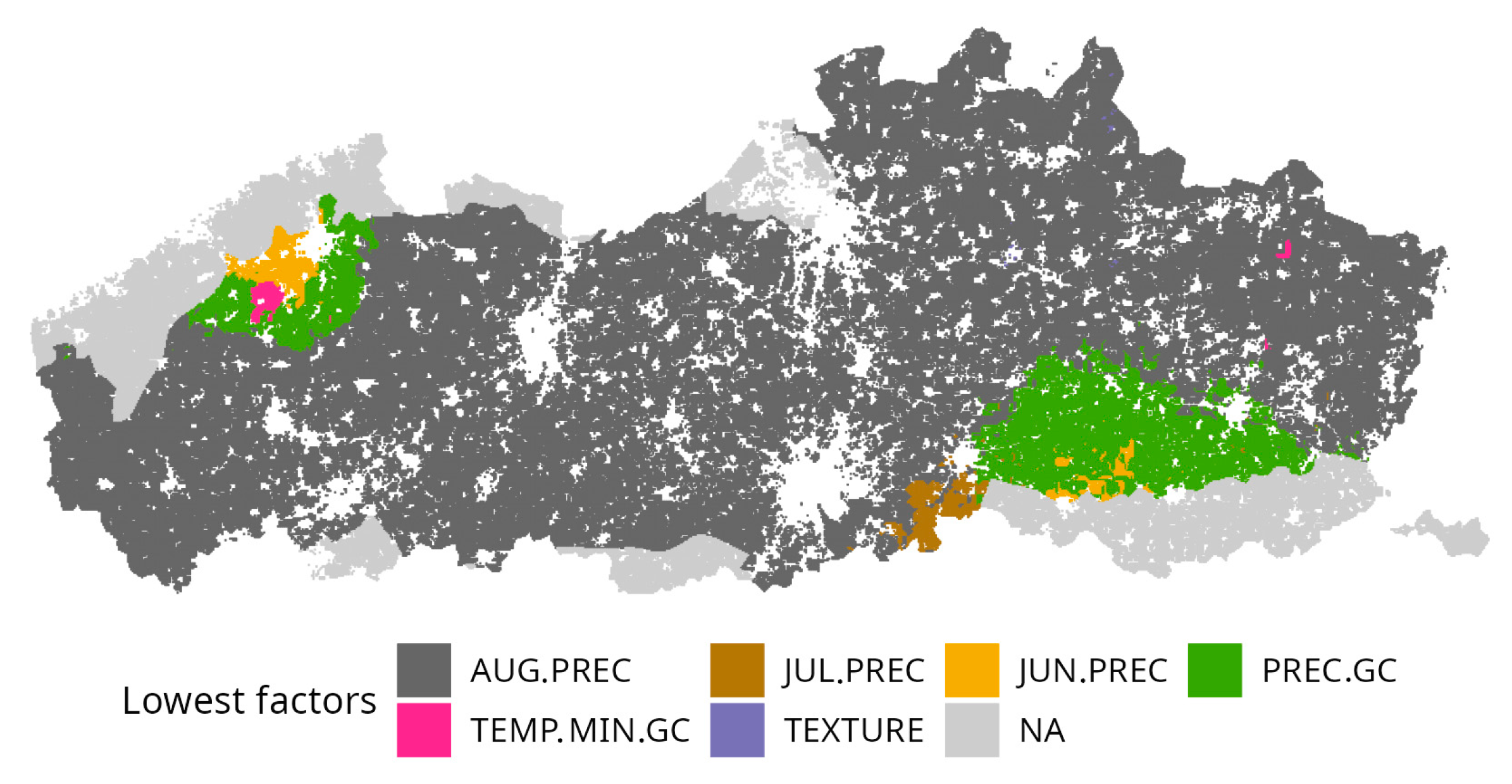
3.2. Limiting Factors Assessment
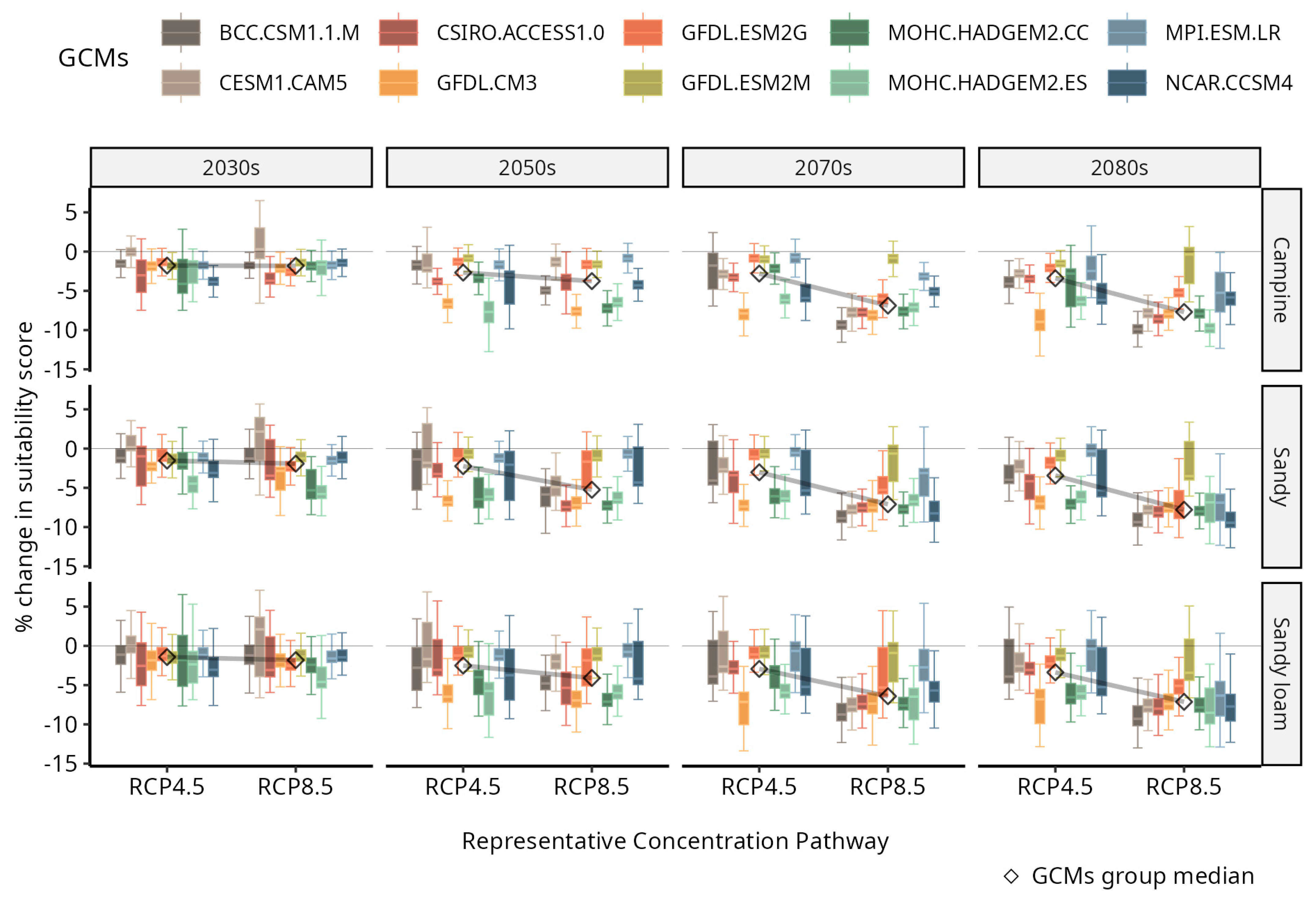
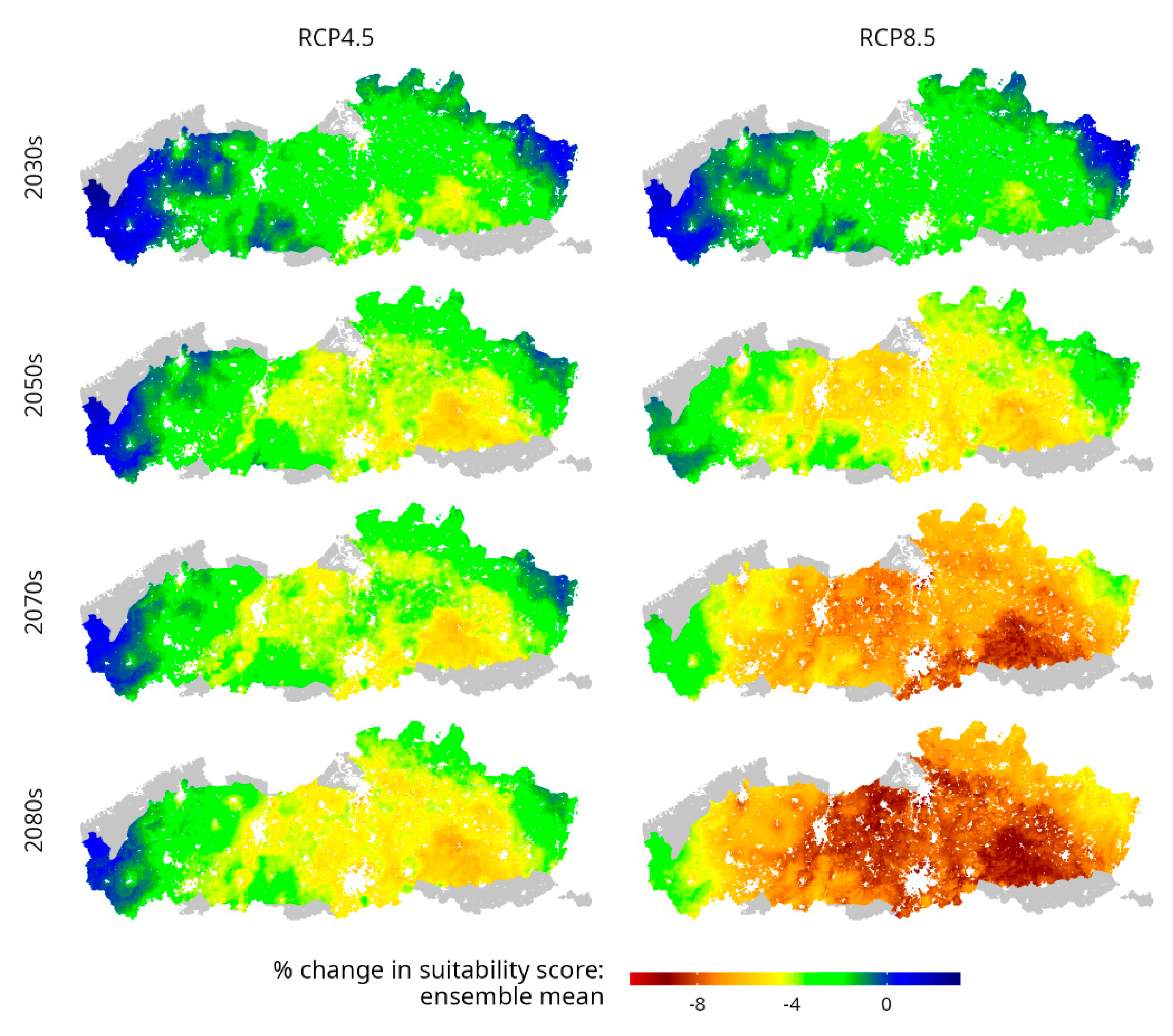
3.3. Future LSA under Climate Change
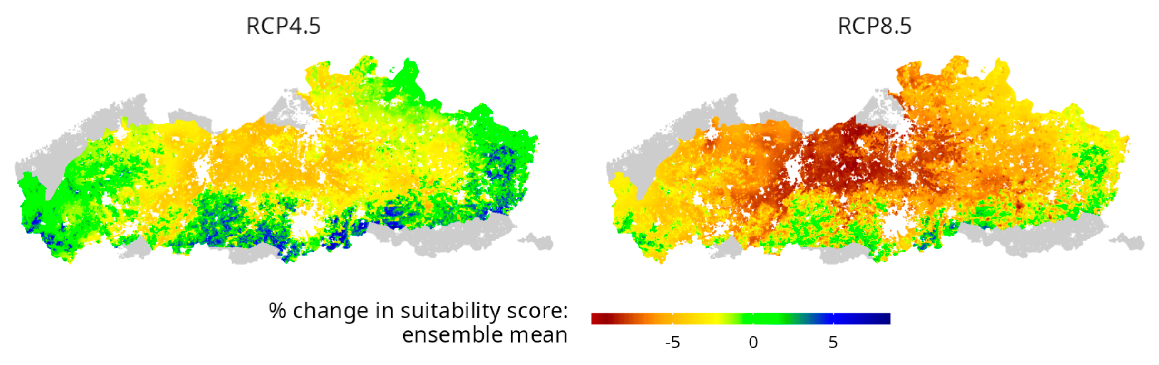
3.4. Future LSA under SICS
4. Discussion
4.1. Data-Related Implications
4.2. LSA Implications
4.3. Future-Climate Modeling Implications
4.4. SICS-Related Implications
5. Conclusions
- The marginal suitability for maize (mostly S3 class) resulting from the current Land Suitability Analysis (LSA) showed that climate, and specifically precipitation, is the major limiting factor for suitability.
- The potential of improved Crop Residue Management (CRM-SICS) to mitigate the impact of future climate change on suitability was investigated by applying the CRM-SICS scenario to the future LSA process and was found to be significant under both RCPs adopted (low or high emissions scenarios) and in all the three main agricultural regions.
- Among the main agricultural regions, the Sandy Loam region shows the strongest response to the long-term application of CRM-SICS for a period of 80 years, up to 2099.
Supplementary Materials
Author Contributions
Funding
Data Availability Statement
Conflicts of Interest
References
- Mugiyo, H.; Chimonyo, V.G.P.; Sibanda, M.; Kunz, R.; Masemola, C.R.; Modi, A.T.; Mabhaudhi, T. Evaluation of Land Suitability Methods with Reference to Neglected and Underutilised Crop Species: A Scoping Review. Land 2021, 10, 125. [Google Scholar] [CrossRef]
- Akpoti, K.; Kabo-bah, A.T.; Zwart, S.J. Agricultural Land Suitability Analysis: State-of-the-Art and Outlooks for Integration of Climate Change Analysis. Agric. Syst. 2019, 173, 172–208. [Google Scholar] [CrossRef]
- Aertsens, J.; De Nocker, L.; Gobin, A. Valuing the Carbon Sequestration Potential for European Agriculture. Land Use Policy 2013, 31, 584–594. [Google Scholar] [CrossRef]
- Hessel, R.; Wyseure, G.; Panagea, I.S.; Alaoui, A.; Reed, M.S.; van Delden, H.; Muro, M.; Mills, J.; Oenema, O.; Areal, F.; et al. Soil-Improving Cropping Systems for Sustainable and Profitable Farming in Europe. Land 2022, 11, 780. [Google Scholar] [CrossRef]
- Magdoff, F.; Van Es, H. Building Soils for Better Crops: Ecological Management for Healthy Soils; Sustainable Agriculture Research & Education (Program), National Institute of Food and Agriculture (U.S.): Beltsville, MD, USA, 2021; ISBN 9781888626193. [Google Scholar]
- Wang, X.; He, C.; Liu, B.; Zhao, X.; Liu, Y.; Wang, Q.; Zhang, H. Effects of Residue Returning on Soil Organic Carbon Storage and Sequestration Rate in China’s Croplands: A Meta-Analysis. Agronomy 2020, 10, 691. [Google Scholar] [CrossRef]
- Malczewski, J. GIS-Based Land-Use Suitability Analysis: A Critical Overview. Prog. Plan. 2004, 62, 3–65. [Google Scholar] [CrossRef]
- FAO. Land Evaluation towards a Revised Framework Land Evaluation towards a Revised Framework Land Evaluation towards a Revised Framework. 2007. Available online: https://edepot.wur.nl/488269 (accessed on 11 December 2023).
- Greene, R.; Devillers, R.; Luther, J.E.; Eddy, B.G. GIS-Based Multiple-Criteria Decision Analysis. Geogr. Compass 2011, 5, 412–432. [Google Scholar] [CrossRef]
- Bagherzadeh, A.; Ghadiri, E.; Souhani Darban, A.R.; Gholizadeh, A. Land Suitability Modeling by Parametric-Based Neural Networks and Fuzzy Methods for Soybean Production in a Semi-Arid Region. Model. Earth Syst. Environ. 2016, 2, 104. [Google Scholar] [CrossRef]
- Olsen, K.; Svenning, J.C.; Balslev, H. Climate Change Is Driving Shifts in Dragonfly Species Richness across Europe via Differential Dynamics of Taxonomic and Biogeographic Groups. Diversity 2022, 14, 1066. [Google Scholar] [CrossRef]
- Liambila, R.N.; Kibret, K. Climate Change Impact on Land Suitability for Rainfed Crop Production in Lake Haramaya Watershed, Eastern Ethiopia. J. Earth Sci. Clim. Chang. 2016, 7, 343. [Google Scholar] [CrossRef]
- Wallach, D.; Mearns, L.O.; Ruane, A.C.; Rötter, R.P.; Asseng, S. Lessons from Climate Modeling on the Design and Use of Ensembles for Crop Modeling. Clim. Chang. 2016, 139, 551–564. [Google Scholar] [CrossRef] [PubMed]
- Zhuang, X.W.; Li, Y.P.; Huang, G.H.; Liu, J. Assessment of Climate Change Impacts on Watershed in Cold-Arid Region: An Integrated Multi-GCM-Based Stochastic Weather Generator and Stepwise Cluster Analysis Method. Clim. Dyn. 2016, 47, 191–209. [Google Scholar] [CrossRef]
- Moss, R.H.; Edmonds, J.A.; Hibbard, K.A.; Manning, M.R.; Rose, S.K.; Van Vuuren, D.P.; Carter, T.R.; Emori, S.; Kainuma, M.; Kram, T.; et al. The next Generation of Scenarios for Climate Change Research and Assessment. Nature 2010, 463, 747–756. [Google Scholar] [CrossRef] [PubMed]
- Wang, B.; Zheng, L.; Liu, D.L.; Ji, F.; Clark, A.; Yu, Q. Using Multi-Model Ensembles of CMIP5 Global Climate Models to Reproduce Observed Monthly Rainfall and Temperature with Machine Learning Methods in Australia. Int. J. Climatol. 2018, 38, 4891–4902. [Google Scholar] [CrossRef]
- Bonfante, A.; Monaco, E.; Alfieri, S.M.; De Lorenzi, F.; Manna, P.; Basile, A.; Bouma, J. Climate Change Effects on the Suitability of an Agricultural Area to Maize Cultivation: Application of a New Hybrid Land Evaluation System. Adv. Agron. 2015, 133, 33–69. [Google Scholar] [CrossRef]
- Iizumi, T.; Ramankutty, N. How Do Weather and Climate Influence Cropping Area and Intensity? Glob. Food Secur. 2015, 4, 46–50. [Google Scholar] [CrossRef]
- Ramirez-Villegas, J.; Jarvis, A.; Läderach, P. Empirical Approaches for Assessing Impacts of Climate Change on Agriculture: The EcoCrop Model and a Case Study with Grain Sorghum. Agric. For. Meteorol. 2013, 170, 67–78. [Google Scholar] [CrossRef]
- Bassu, S.; Brisson, N.; Durand, J.L.; Boote, K.; Lizaso, J.; Jones, J.W.; Rosenzweig, C.; Ruane, A.C.; Adam, M.; Baron, C.; et al. How Do Various Maize Crop Models Vary in Their Responses to Climate Change Factors? Glob. Chang. Biol. 2014, 20, 2301–2320. [Google Scholar] [CrossRef]
- Kriticos, D.J.; Murphy, H.T.; Jovanovic, T.; Taylor, J.; Herr, A.; Raison, J.; O’Connell, D. Balancing Bioenergy and Biosecurity Policies: Estimating Current and Future Climate Suitability Patterns for a Bioenergy Crop. GCB Bioenergy 2014, 6, 587–598. [Google Scholar] [CrossRef]
- Ramirez-Cabral, N.Y.Z.; Kumar, L.; Shabani, F. Global Alterations in Areas of Suitability for Maize Production from Climate Change and Using a Mechanistic Species Distribution Model (CLIMEX). Sci. Rep. 2017, 7, 5910. [Google Scholar] [CrossRef]
- Nguyen, T.T.; Verdoodt, A.; Van, Y.T.; Delbecque, N.; Tran, T.C.; Van Ranst, E. Design of a GIS and Multi-Criteria Based Land Evaluation Procedure for Sustainable Land-Use Planning at the Regional Level. Agric. Ecosyst. Environ. 2015, 200, 1–11. [Google Scholar] [CrossRef]
- de Frutos Cachorro, J.; Gobin, A.; Buysse, J. Farm-Level Adaptation to Climate Change: The Case of the Loam Region in Belgium. Agric. Syst. 2018, 165, 164–176. [Google Scholar] [CrossRef]
- Geopunt Vlaanderen. Available online: https://www.vlaanderen.be/datavindplaats/catalogus/landbouwstreken-belgie-toestand-1974-02-15 (accessed on 17 October 2023).
- Gobin, A. Impact of Heat and Drought Stress on Arable Crop Production in Belgium. Nat. Hazards Earth Syst. Sci. 2012, 12, 1911–1922. [Google Scholar] [CrossRef]
- Dondeyne, S.; Vanierschot, L.; Langohr, R.; Van Ranst, E.; Deckers, J. The Soil Map of the Flemish Region Converted to the 3rd Edition of the World Reference Base for Soil Resources. 2014. Available online: https://www.researchgate.net/publication/267969329_The_soil_map_of_the_Flemish_region_converted_to_the_3rd_edition_of_the_World_Reference_Base_for_soil_resources?channel=doi&linkId=545ded7f0cf2c1a63bfaecc2&showFulltext=true (accessed on 11 December 2023).
- Hengl, T.; De Jesus, J.M.; Heuvelink, G.B.M.; Gonzalez, M.R.; Kilibarda, M.; Blagotić, A.; Shangguan, W.; Wright, M.N.; Geng, X.; Bauer-Marschallinger, B.; et al. SoilGrids250m: Global Gridded Soil Information Based on Machine Learning. PLoS ONE 2017, 12, e0169748. [Google Scholar] [CrossRef] [PubMed]
- Muñoz-Sabater, J.; Dutra, E.; Agustí-Panareda, A.; Albergel, C.; Arduini, G.; Balsamo, G.; Boussetta, S.; Choulga, M.; Harrigan, S.; Hersbach, H.; et al. ERA5-Land: A State-of-the-Art Global Reanalysis Dataset for Land Applications. Earth Syst. Sci. Data 2021, 13, 4349–4383. [Google Scholar] [CrossRef]
- Abatzoglou, J.T.; Dobrowski, S.Z.; Parks, S.A.; Hegewisch, K.C. TerraClimate, a High-Resolution Global Dataset of Monthly Climate and Climatic Water Balance from 1958–2015. Sci. Data 2018, 5, 170191. [Google Scholar] [CrossRef]
- Navarro-Racines, C.; Tarapues, J.; Thornton, P.; Jarvis, A.; Ramirez-Villegas, J. High-Resolution and Bias-Corrected CMIP5 Projections for Climate Change Impact Assessments. Sci. Data 2020, 7, 7. [Google Scholar] [CrossRef]
- Zhang, L.; Liu, G.; Yang, Y.; Guo, X.; Jin, S.; Xie, R.; Ming, B.; Xue, J.; Wang, K.; Li, S.; et al. Root Characteristics for Maize with the Highest Grain Yield Potential of 22.5 Mg Ha−1 in China. Agriculture 2023, 13, 765. [Google Scholar] [CrossRef]
- Bilas, G.; Karapetsas, N.; Gobin, A.; Mesdanitis, K.; Toth, G.; Hermann, T.; Wang, Y.; Luo, L.; Koutsos, T.M.; Moshou, D.; et al. Land Suitability Analysis as a Tool for Evaluating Soil-Improving Cropping Systems. Land 2022, 11, 2200. [Google Scholar] [CrossRef]
- Asaad, A.-A.B.; Salvacion, A.R.; Yen, B.T. ALUES: R Package for Agricultural Land Use Evaluation System. J. Open Source Softw. 2022, 7, 4228. [Google Scholar] [CrossRef]
- Taylor, K.E.; Stouffer, R.J.; Meehl, G.A. An Overview of CMIP5 and the Experiment Design. Bull. Am. Meteorol. Soc. 2012, 93, 485–498. [Google Scholar] [CrossRef]
- McSweeney, C.F.; Jones, R.G.; Lee, R.W.; Rowell, D.P. Selecting CMIP5 GCMs for Downscaling over Multiple Regions. Clim. Dyn. 2015, 44, 3237–3260. [Google Scholar] [CrossRef]
- Xin, X.; Zhang, L.; Zhang, J.; Wu, T.; Fang, Y. Climate Change Projections over East Asia with BBC_CSM1.1 Climate Model under RCP Scenarios. J. Meteorol. Soc. Jpn. 2013, 91, 413–429. [Google Scholar] [CrossRef]
- Bi, D.; Dix, M.; Marsland, S.J.; O’Farrell, S.; Rashid, H.A.; Uotila, P.; Hirst, A.C.; Kowalczyk, E.; Golebiewski, M.; Sullivan, A.; et al. The ACCESS Coupled Model: Description, Control Climate and Evaluation. Aust. Meteorol. Oceanogr. J. 2013, 63, 41–64. [Google Scholar] [CrossRef]
- Hurrell, J.W.; Holland, M.M.; Gent, P.R.; Ghan, S.; Kay, J.E.; Kushner, P.J.; Lamarque, J.F.; Large, W.G.; Lawrence, D.; Lindsay, K.; et al. The Community Earth System Model: A Framework for Collaborative Research. Bull. Am. Meteorol. Soc. 2013, 94, 1339–1360. [Google Scholar] [CrossRef]
- Donner, L.J.; Wyman, B.L.; Hemler, R.S.; Horowitz, L.W.; Ming, Y.; Zhao, M.; Golaz, J.C.; Ginoux, P.; Lin, S.J.; Schwarzkopf, M.D.; et al. The Dynamical Core, Physical Parameterizations, and Basic Simulation Characteristics of the Atmospheric Component AM3 of the GFDL Global Coupled Model CM3. J. Clim. 2011, 24, 3484–3519. [Google Scholar] [CrossRef]
- Dunne, J.P.; John, J.G.; Shevliakova, E.; Stouffer, R.J.; Krasting, J.P.; Malyshev, S.L.; Milly, P.C.D.; Sentman, L.T.; Adcroft, A.J.; Cooke, W.; et al. GFDL’s ESM2 Global Coupled Climate-Carbon Earth System Models. Part II: Carbon System Formulation and Baseline Simulation Characteristics*. J. Clim. 2013, 26, 2247–2267. [Google Scholar] [CrossRef]
- Martin, G.M.; Bellouin, N.; Collins, W.J.; Culverwell, I.D.; Halloran, P.R.; Hardiman, S.C.; Hinton, T.J.; Jones, C.D.; McDonald, R.E.; McLaren, A.J.; et al. The HadGEM2 Family of Met Office Unified Model Climate Configurations. Geosci. Model Dev. 2011, 4, 723–757. [Google Scholar] [CrossRef]
- Reick, C.H.; Raddatz, T.; Brovkin, V.; Gayler, V. Representation of Natural and Anthropogenic Land Cover Change in MPI-ESM. J. Adv. Model. Earth Syst. 2013, 5, 459–482. [Google Scholar] [CrossRef]
- Gent, P.R.; Danabasoglu, G.; Donner, L.J.; Holland, M.M.; Hunke, E.C.; Jayne, S.R.; Lawrence, D.M.; Neale, R.B.; Rasch, P.J.; Vertenstein, M.; et al. The Community Climate System Model Version 4. J. Clim. 2011, 24, 4973–4991. [Google Scholar] [CrossRef]
- van Vuuren, D.P.; Edmonds, J.; Kainuma, M.; Riahi, K.; Thomson, A.; Hibbard, K.; Hurtt, G.C.; Kram, T.; Krey, V.; Lamarque, J.F.; et al. The Representative Concentration Pathways: An Overview. Clim. Chang. 2011, 109, 5–31. [Google Scholar] [CrossRef]
- Jebeile, J.; Barberousse, A. Model Spread and Progress in Climate Modelling. Eur. J. Philos. Sci. 2021, 11, 66. [Google Scholar] [CrossRef]
- Yip, S.; Ferro, C.A.T.; Stephenson, D.B.; Hawkins, E. A Simple, Coherent Framework for Partitioning Uncertainty in Climate Predictions. J. Clim. 2011, 24, 4634–4643. [Google Scholar] [CrossRef]
- Murakami, D.; Griffith, D.A. Random Effects Specifications in Eigenvector Spatial Filtering: A Simulation Study. J. Geogr. Syst. 2015, 17, 311–331. [Google Scholar] [CrossRef]
- Chun, Y.; Griffith, D.A. A Quality Assessment of Eigenvector Spatial Filtering Based Parameter Estimates for the Normal Probability Model. Spat. Stat. 2014, 10, 1–11. [Google Scholar] [CrossRef]
- Murakami, D.; Griffith, D.A. A Memory-Free Spatial Additive Mixed Modeling for Big Spatial Data. Jpn. J. Stat. Data Sci. 2020, 3, 215–241. [Google Scholar] [CrossRef]
- Murakami, D. Spmoran: An R Package for Moran’s Eigenvector-Based Spatial Regression Analysis (Version 2017/06). 2017. Available online: https://cran.r-hub.io/web/packages/spmoran/vignettes/vignettes.pdf (accessed on 11 December 2023).
- Anselin, L.; Rey, S. Properties of Tests for Spatial Dependence in Linear Regression Models. Geogr. Anal. 1991, 23, 112–131. [Google Scholar] [CrossRef]
- Van De Vreken, P.; Gobin, A.; Baken, S.; Van Holm, L.; Verhasselt, A.; Smolders, E.; Merckx, R. Crop Residue Management and Oxalate-Extractable Iron and Aluminium Explain Long-Term Soil Organic Carbon Sequestration and Dynamics. Eur. J. Soil Sci. 2016, 67, 332–340. [Google Scholar] [CrossRef]
- Nadeu, E.; Gobin, A.; Fiener, P.; van Wesemael, B.; van Oost, K. Modelling the Impact of Agricultural Management on Soil Carbon Stocks at the Regional Scale: The Role of Lateral Fluxes. Glob. Chang. Biol. 2015, 21, 3181–3192. [Google Scholar] [CrossRef]
- Bolinder, M.A.; Crotty, F.; Elsen, A.; Frac, M.; Kismányoky, T.; Lipiec, J.; Tits, M.; Tóth, Z.; Kätterer, T. The Effect of Crop Residues, Cover Crops, Manures and Nitrogen Fertilization on Soil Organic Carbon Changes in Agroecosystems: A Synthesis of Reviews. Mitig. Adapt. Strateg. Glob. Chang. 2020, 25, 929–952. [Google Scholar] [CrossRef]
- Peng, Y.; Rieke, E.L.; Chahal, I.; Norris, C.E.; Janovicek, K.; Mitchell, J.P.; Roozeboom, K.L.; Hayden, Z.D.; Strock, J.S.; Machado, S.; et al. Maximizing Soil Organic Carbon Stocks under Cover Cropping: Insights from Long-Term Agricultural Experiments in North America. Agric. Ecosyst. Environ. 2023, 356, 108599. [Google Scholar] [CrossRef]
- Zamani, S.; Gobin, A.; Van de Vyver, H.; Gerlo, J. Atmospheric Drought in Belgium—Statistical Analysis of Precipitation Deficit. Int. J. Climatol. 2016, 36, 3056–3071. [Google Scholar] [CrossRef]
- Gobin, A.; Van de Vyver, H. Spatio-Temporal Variability of Dry and Wet Spells and Their Influence on Crop Yields. Agric. For. Meteorol. 2021, 308–309, 108565. [Google Scholar] [CrossRef]
- Vanwindekens, F.M.; Gobin, A.; Curnel, Y.; Planchon, V. New Approach for Mapping the Vulnerability of Agroecosystems Based on Expert Knowledge. Math. Geosci. 2018, 50, 679–696. [Google Scholar] [CrossRef]
- Poggio, L.; De Sousa, L.M.; Batjes, N.H.; Heuvelink, G.B.M.; Kempen, B.; Ribeiro, E.; Rossiter, D. SoilGrids 2.0: Producing Soil Information for the Globe with Quantified Spatial Uncertainty. SOIL 2021, 7, 217–240. [Google Scholar] [CrossRef]
- Richer-de-Forges, A.C.; Arrouays, D.; Poggio, L.; Chen, S.; Lacoste, M.; Minasny, B.; Libohova, Z.; Roudier, P.; Mulder, V.L.; Nédélec, H.; et al. Hand-Feel Soil Texture Observations to Evaluate the Accuracy of Digital Soil Maps for Local Prediction of Soil Particle Size Distribution: A Case Study in Central France. Pedosphere 2023, 33, 731–743. [Google Scholar] [CrossRef]
- Batjes, N.H.; Ribeiro, E.; Van Oostrum, A. Standardised Soil Profile Data to Support Global Mapping and Modelling (WoSIS Snapshot 2019). Earth Syst. Sci. Data 2020, 12, 299–320. [Google Scholar] [CrossRef]
- Zhang, J.; Su, Y.; Wu, J.; Liang, H. GIS Based Land Suitability Assessment for Tobacco Production Using AHP and Fuzzy Set in Shandong Province of China. Comput. Electron. Agric. 2015, 114, 202–211. [Google Scholar] [CrossRef]
- Brandt, P.; Kvakić, M.; Butterbach-Bahl, K.; Rufino, M.C. How to Target Climate-Smart Agriculture? Concept and Application of the Consensus-Driven Decision Support Framework “TargetCSA”. Agric. Syst. 2017, 151, 234–245. [Google Scholar] [CrossRef]
- Hu, X.; Fan, H.; Cai, M.; Sejas, S.A.; Taylor, P.; Yang, S. A Less Cloudy Picture of the Inter-Model Spread in Future Global Warming Projections. Nat. Commun. 2020, 11, 4472. [Google Scholar] [CrossRef]
- Cattiaux, J.; Douville, H.; Peings, Y. European Temperatures in CMIP5: Origins of Present-Day Biases and Future Uncertainties. Clim. Dyn. 2013, 41, 2889–2907. [Google Scholar] [CrossRef]
- Trnka, M.; Olesen, J.E.; Kersebaum, K.C.; Skjelvåg, A.O.; Eitzinger, J.; Seguin, B.; Peltonen-Sainio, P.; Rötter, R.; Iglesias, A.; Orlandini, S.; et al. Agroclimatic Conditions in Europe under Climate Change. Glob. Chang. Biol. 2011, 17, 2298–2318. [Google Scholar] [CrossRef]
- Zhao, J.; Bindi, M.; Eitzinger, J.; Ferrise, R.; Gaile, Z.; Gobin, A.; Holzkämper, A.; Kersebaum, K.C.; Kozyra, J.; Kriaučiūnienė, Z.; et al. Priority for Climate Adaptation Measures in European Crop Production Systems. Eur. J. Agron. 2022, 138, 126516. [Google Scholar] [CrossRef]
- Aguilera, E.; Lassaletta, L.; Gattinger, A.; Gimeno, B.S. Managing Soil Carbon for Climate Change Mitigation and Adaptation in Mediterranean Cropping Systems: A Meta-Analysis. Agric. Ecosyst. Environ. 2013, 168, 25–36. [Google Scholar] [CrossRef]


| Campine | Sandy | Sandy Loam | ||||||||||
|---|---|---|---|---|---|---|---|---|---|---|---|---|
| Raster Data | Min | Max | Mean | sd | Min | Max | Mean | sd | Min | Max | Mean | sd |
| Soil | ||||||||||||
| BD | 1.15 | 1.54 | 1.43 | 0.05 | 1.12 | 1.55 | 1.41 | 0.048 | 1.23 | 1.63 | 1.47 | 0.047 |
| CEC | 5.51 | 28.8 | 12.7 | 2.44 | 9.84 | 35.1 | 19.1 | 4.87 | 9.74 | 32.7 | 14.5 | 2.86 |
| CRFVOL | 1.8 | 18.6 | 6.71 | 1.88 | 3.47 | 20.8 | 6.55 | 1.67 | 4.04 | 23 | 8.88 | 3.3 |
| CLAY | 2.57 | 32.6 | 15 | 6.07 | 7.29 | 37.9 | 21.1 | 4.31 | 10.8 | 37.7 | 22.9 | 2.9 |
| PH | 3.88 | 7.97 | 5.27 | 0.272 | 3.91 | 8.27 | 5.92 | 0.414 | 3.95 | 8.83 | 6.36 | 0.516 |
| SAND | 11.2 | 93.7 | 57.3 | 18.8 | 10.5 | 82.1 | 45.4 | 10.6 | 8.75 | 71.4 | 27.9 | 9.07 |
| SILT | 2.95 | 70.2 | 27.7 | 13.8 | 9.93 | 69.1 | 33.4 | 7.83 | 16.5 | 73.8 | 49.1 | 8.56 |
| SOC | 6.33 | 77.8 | 16.8 | 6.13 | 5.2 | 116 | 19.1 | 8.09 | 3.68 | 68.5 | 12.5 | 4.72 |
| Climate | ||||||||||||
| MAY.PREC | 55 | 70 | 62.2 | 2.39 | 53 | 66 | 60.6 | 2.26 | 49 | 70 | 61.5 | 3.84 |
| JUN.PREC | 70 | 82 | 75.9 | 2.08 | 61 | 82 | 72.9 | 3.48 | 56 | 80 | 71.5 | 4.71 |
| JUL.PREC | 63 | 81 | 72.6 | 3.09 | 62 | 74 | 68.1 | 1.52 | 56 | 78 | 67.5 | 4.24 |
| AUG.PREC | 54 | 73 | 62.3 | 3.5 | 53 | 71 | 60.1 | 2.76 | 51 | 75 | 59.8 | 5.68 |
| PREC.GC | 249 | 301 | 273 | 9.43 | 234 | 284 | 262 | 6.39 | 214 | 298 | 260 | 16.7 |
| TEMP.AVG.GC | 15.9 | 17 | 16.2 | 0.179 | 15.2 | 16.9 | 16.1 | 0.4 | 14.9 | 17 | 16 | 0.464 |
| TEMP.MIN.GC | 11.5 | 13.4 | 12.3 | 0.267 | 11.5 | 13.2 | 12.4 | 0.402 | 11.3 | 13.3 | 12.3 | 0.453 |
| Topography | ||||||||||||
| SLP | 0 | 15.6 | 0.502 | 0.757 | 0 | 11 | 0.482 | 0.726 | 0 | 13 | 1.64 | 1.53 |
| Model (Reference) | Institute | RCP | |||
|---|---|---|---|---|---|
| 2.6 | 4.5 | 6.0 | 8.5 | ||
| BCC-CSM1.1(m) [37] | Beijing Climate Center and China Meteorological Administration | ● | ● | ● | ● |
| CSIRO-ACCESS1.0 [38] | Commonwealth Scientific and Industrial Research Organization (CSIRO) and Bureau of Meteorology (BOM), Australia | ● | ● | ||
| CESM1-CAM5 [39] | National Science Foundation, U.S. Department of Energy, and National Center for Atmospheric Research (NCAR) | ● | ● | ● | ● |
| GFDL-CM3 [40] | NOAA Geophysical Fluid Dynamics Laboratory | ● | ● | ● | ● |
| GFDL-ESM2G [41] | ● | ● | ● | ● | |
| GFDL-ESM2M [41] | ● | ● | ● | ● | |
| MOHC-HadGEM2-CC [42] | UK Met Office Hadley Centre | ● | ● | ||
| MOHC-HadGEM2-ES [42] | ● | ● | ● | ● | |
| MPI-ESM-LR [43] | Max Planck Institute for Meteorology | ● | ● | ● | |
| NCAR-CCSM4 [44] | US National Centre for Atmospheric Research | ● | ● | ● | ● |
| Region | n (Cells) | Total Response Variance 1 | Spatial Dependence Kernel |
Moran Eigenvectors (n) |
Computational Time (Minutes) 2 |
Scaled MC [Moran.I/ Max (Moran.I)] |
|---|---|---|---|---|---|---|
| Campine | 3.90 × 10⁶ | 9.355 | Exponential | 500 | 43 | 0.6836812 |
| Sandy | 3.514 × 10⁶ | 10.76 | Gaussian | 500 | 32 | 0.6570547 |
| Sandy Loam | 4.453 × 10⁶ | 11.42 | Spherical | 1000 | 89 | 0.6463084 |
| Region | GCM | RCP | Future Period | GCM:RCP | GCM:Future Period | RCP:Future Period | S | e | Proportion (%) of Variance Explained |
|---|---|---|---|---|---|---|---|---|---|
| Campine | 26.58 | 6.77 | 19.70 | 4.95 | 9.79 | 5.75 | 12.22 | 14.25 | 85.75 |
| Sandy | 27.03 | 10.91 | 16.19 | 3.73 | 5.72 | 3.53 | 11.12 | 21.78 | 78.22 |
| Sandy Loam | 19.77 | 7.31 | 14.79 | 2.95 | 5.30 | 3.80 | 26.68 | 19.39 | 80.61 |
| Future Period | RCP | Agricultural Region | n (Cells) | Min | Max | Median | Quant.1 | Quant.3 | IQR | Mean |
|---|---|---|---|---|---|---|---|---|---|---|
| Ensemble mean | ||||||||||
| 2080s | RCP8.5 | Sandy Loam | 55,664 | −9.776 | −1.483 | −6.290 | −7.233 | −5.061 | 2.172 | −6.012 |
| 2080s | RCP8.5 | Sandy | 43,931 | −10.06 | −3.357 | −7.449 | −8.071 | −6.242 | 1.829 | −7.152 |
| 2080s | RCP8.5 | Campine | 48,745 | −9.610 | −3.083 | −6.431 | −7.379 | −5.617 | 1.762 | −6.406 |
| Ensemble standard deviation | ||||||||||
| 2080s | RCP8.5 | Sandy Loam | 55,664 | 1.515 | 6.194 | 2.524 | 2.264 | 2.878 | 0.615 | 2.675 |
| 2080s | RCP8.5 | Sandy | 43,931 | 1.389 | 5.607 | 2.121 | 1.883 | 2.663 | 0.780 | 2.265 |
| 2080s | RCP8.5 | Campine | 48,745 | 1.761 | 5.102 | 3.061 | 2.366 | 3.338 | 0.972 | 2.897 |
| Region | Climate Change Impact | Uncertainty from GCMs Ensemble Modeling | CRM Mitigation Gain (80-Year Application) |
|---|---|---|---|
| Campine | −6.406 | 2.897 | 2.564 |
| Sandy | −7.152 | 2.265 | 0.694 |
| Sandy Loam | −6.012 | 2.675 | 3.421 |
Disclaimer/Publisher’s Note: The statements, opinions and data contained in all publications are solely those of the individual author(s) and contributor(s) and not of MDPI and/or the editor(s). MDPI and/or the editor(s) disclaim responsibility for any injury to people or property resulting from any ideas, methods, instructions or products referred to in the content. |
© 2024 by the authors. Licensee MDPI, Basel, Switzerland. This article is an open access article distributed under the terms and conditions of the Creative Commons Attribution (CC BY) license (https://creativecommons.org/licenses/by/4.0/).
Share and Cite
Karapetsas, N.; Gobin, A.; Bilas, G.; Koutsos, T.M.; Pavlidis, V.; Katragkou, E.; Alexandridis, T.K. Analysis of Land Suitability for Maize Production under Climate Change and Its Mitigation Potential through Crop Residue Management. Land 2024, 13, 63. https://doi.org/10.3390/land13010063
Karapetsas N, Gobin A, Bilas G, Koutsos TM, Pavlidis V, Katragkou E, Alexandridis TK. Analysis of Land Suitability for Maize Production under Climate Change and Its Mitigation Potential through Crop Residue Management. Land. 2024; 13(1):63. https://doi.org/10.3390/land13010063
Chicago/Turabian StyleKarapetsas, Nikolaos, Anne Gobin, George Bilas, Thomas M. Koutsos, Vasileios Pavlidis, Eleni Katragkou, and Thomas K. Alexandridis. 2024. "Analysis of Land Suitability for Maize Production under Climate Change and Its Mitigation Potential through Crop Residue Management" Land 13, no. 1: 63. https://doi.org/10.3390/land13010063
APA StyleKarapetsas, N., Gobin, A., Bilas, G., Koutsos, T. M., Pavlidis, V., Katragkou, E., & Alexandridis, T. K. (2024). Analysis of Land Suitability for Maize Production under Climate Change and Its Mitigation Potential through Crop Residue Management. Land, 13(1), 63. https://doi.org/10.3390/land13010063