
Mapping an Indicator Species of Sea-Level Rise along the Forest–Marsh Ecotone


Abstract
:1. Introduction
1.1. Coastal Forests and Climate Change
1.2. Atlantic White Cedar Ecosystem Biogeography and Vulnerability
1.3. Predictive Habitat Distribution Modelling
1.4. Research Questions and Objectives
2. Materials and Methods
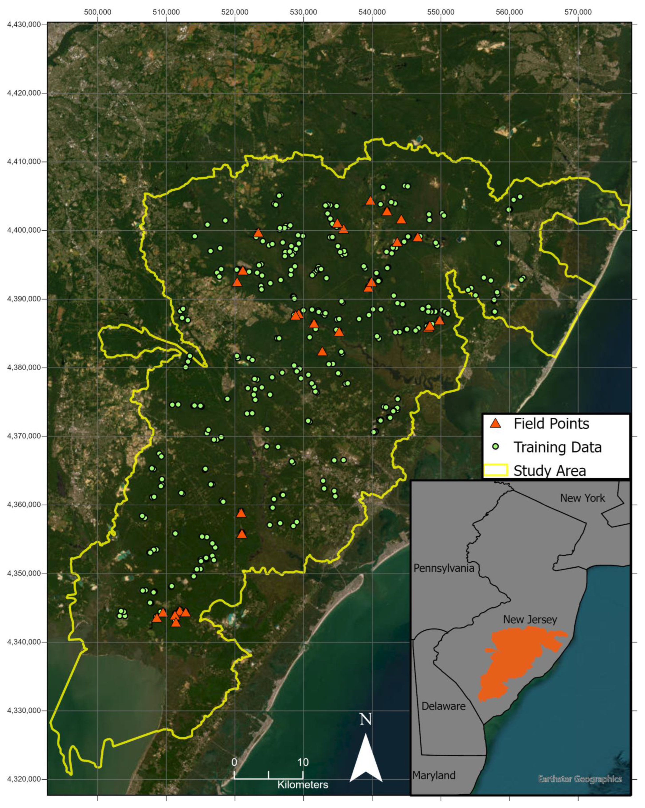
2.1. Study Area
2.2. Sample Data Collection
2.3. Satellite Data
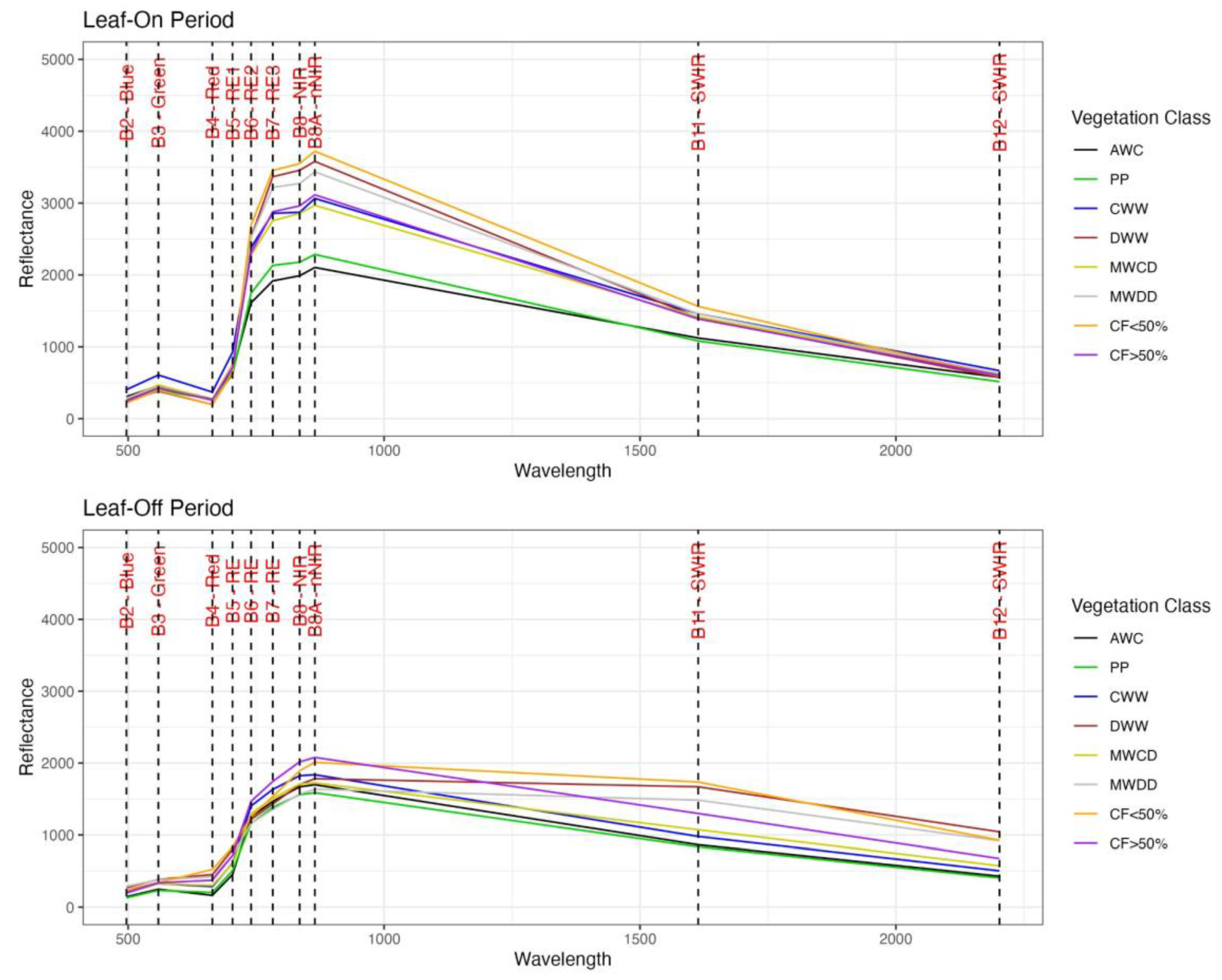
Spectral Signatures and Phenology
2.4. Topographic and Abiotic Data
2.5. Predictive Habitat Distribution Modelling
3. Results
3.1. Spectral Signatures and Phenology
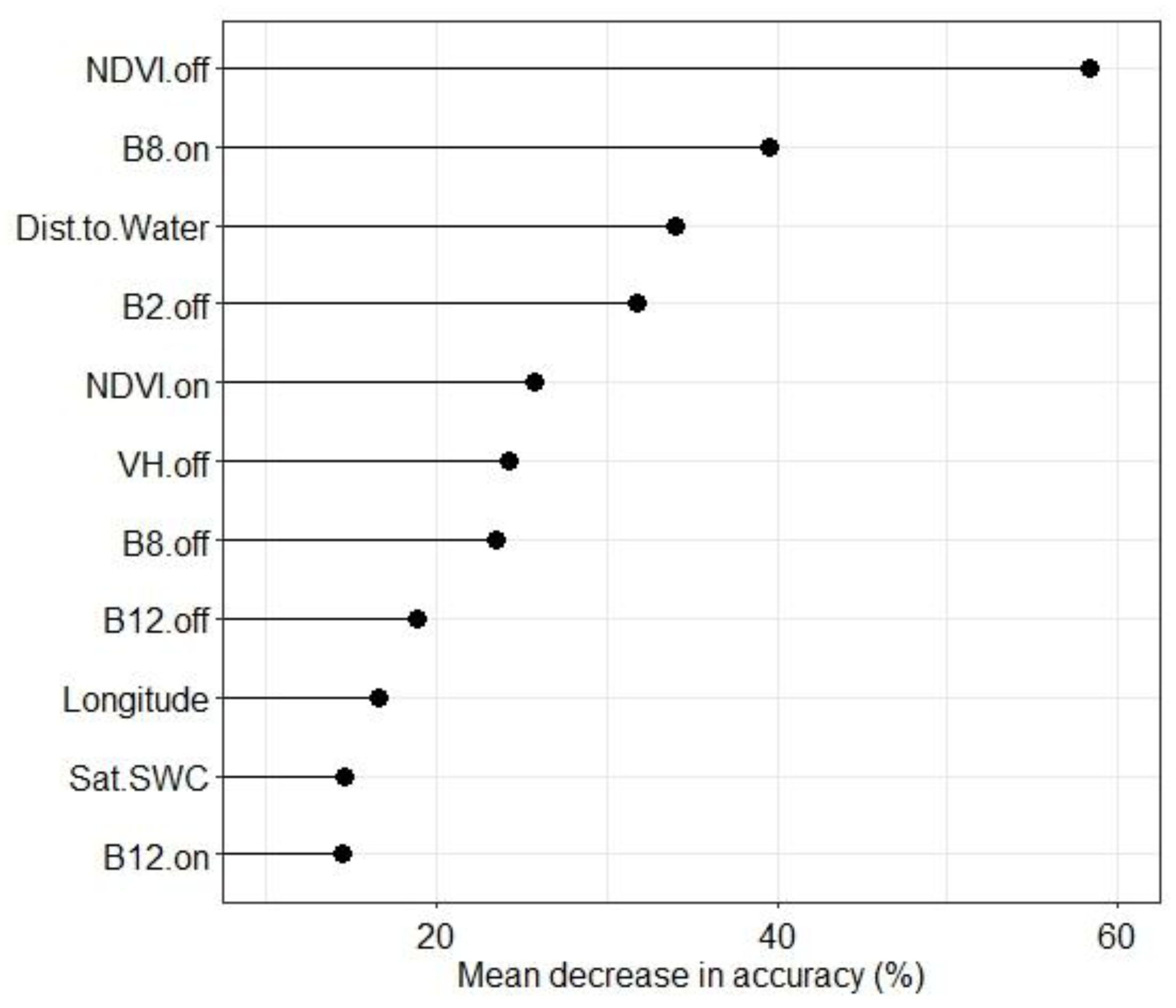
3.2. Species Distribution Model Evaluation
3.3. Atlantic White Cedar Mapping
4. Discussion
4.1. Remote Sensing Is Critical in Mapping Atlantic White Cedar
4.2. Ecological and Technological Considerations
4.3. Management Implications for Atlantic White Cedar
5. Conclusions
Author Contributions
Funding
Data Availability Statement
Acknowledgments
Conflicts of Interest
References
- Schieder, N.W.; Kirwan, M.L. Sea-Level Driven Acceleration in Coastal Forest Retreat. Geology 2019, 47, 1151–1155. [Google Scholar] [CrossRef]
- Jobe, J.G.D.; Gedan, K. Species-Specific Responses of a Marsh-Forest Ecotone Plant Community Responding to Climate Change. Ecology 2021, 102, e03296. [Google Scholar] [CrossRef]
- Fagherazzi, S.; Nordio, G.; Munz, K.; Catucci, D.; Kearney, W.S. Variations in Persistence and Regenerative Zones in Coastal Forests Triggered by Sea Level Rise and Storms. Remote Sens. 2019, 11, 2019. [Google Scholar] [CrossRef]
- Able, K.W. Special Issue: Concepts and Controversies in Tidal Marsh Ecology Revisited From Cedar Cemeteries to Marsh Lakes: A Case Study of Sea-Level Rise and Habitat Change in a Northeastern US Salt Marsh. Estuaries Coasts 2021, 44, 1649–1657. [Google Scholar] [CrossRef]
- Doyle, J.M.; Earley, K.E.; Atkinson, R.B. An Analysis of Atlantic White Cedar (Chaemaecyparis thyoides (L.) B.S.P.) Tree Rings as Indicators of Ghost Forest Development in a Globally Threatened Ecosystem. Forests 2021, 12, 973. [Google Scholar] [CrossRef]
- Hauser, S.; Meixler, M.S.; Laba, M. Quantification of Impacts and Ecosystem Services Loss in New Jersey Coastal Wetlands Due to Hurricane Sandy Storm Surge. Wetlands 2015, 35, 1137–1148. [Google Scholar] [CrossRef]
- Ury, E.A.; Yang, X.; Wright, J.P.; Bernhardt, E.S. Rapid Deforestation of a Coastal Landscape Driven by Sea-Level Rise and Extreme Events. Ecol. Appl. 2021, 31, e02339. [Google Scholar] [CrossRef]
- Woods, N.N.; Swall, J.L.; Zinnert, J.C. Soil Salinity Impacts Future Community Composition of Coastal Forests. Wetlands 2020, 40, 1495–1503. [Google Scholar] [CrossRef]
- Kopp, R.E.; Andrews, C.; Broccoli, A.; Garner, A.; Kreeger, D.; Leichenko, R.; Lin, N.; Little, C.; Miller, J.A.; Miller, J.K.; et al. New Jersey’s Rising Seas and Changing Coastal Storms: Report of the 2019 Science and Technical Advisory Panel; The State University of New Jersey: New Brunswick, NJ, USA, 2019. [Google Scholar]
- Cooper, M.J.P.; Beevers, M.D.; Oppenheimer, M. The Potential Impacts of Sea Level Rise on the Coastal Region of New Jersey, USA. Clim. Chang. 2008, 90, 475–492. [Google Scholar] [CrossRef]
- Smith, A.J.; Goetz, E.M. Climate Change Drives Increased Directional Movement of Landscape Ecotones. Landsc. Ecol. 2021, 36, 3105–3116. [Google Scholar] [CrossRef]
- Hasse, J.E.; Lathrop, R.G.; Bognar, J.A. Changing Landscapes in the Garden State: Land Use Change in NJ 1986 Thru 2012; Rutgers University: New Brunswick, NJ, USA; Rowan University: Glassboro, NJ, USA, 2016. [Google Scholar]
- The American Littoral Society; National Fish and Wildlife Foundation. Assessing the Impacts of Hurricane Sandy. 2012. Available online: https://rucore.libraries.rutgers.edu/rutgers-lib/43631/ (accessed on 19 September 2024).
- Hnatkovich, A.M.; Yorks, T.E. Current Status and Future Development of the Only Chamaecyparis thyoides (Atlantic White-Cedar) Population in Pennsylvania. Nat. Areas J. 2009, 29, 216–223. [Google Scholar] [CrossRef]
- Little, S.J. Ecology and Silviculture of Whitecedar and Associated Hardwoods in Southern New Jersey. Yale Sch. For. Environ. Stud. Bull. Ser. 1950, 54, 134. [Google Scholar]
- Crawford, E.R.; Day, F.P.; Atkinson, R.B. Influence of Environment and Substrate Quality on Root Decomposition in Naturally Regenerating and Restored Atlantic White Cedar Wetlands. Wetlands 2007, 27, 1–11. [Google Scholar] [CrossRef]
- Laing, J.M.; Shear, T.H.; Blazich, F.A. How Management Strategies Have Affected Atlantic White-Cedar Forest Recovery after Massive Wind Damage in the Great Dismal Swamp. For. Ecol. Manag. 2011, 262, 1337–1344. [Google Scholar] [CrossRef]
- Assal, T.J.; Steen, V.A.; Caltrider, T.; Cundy, T.; Stewart, C.; Manning, N.; Anderson, P.J. Monitoring Long-Term Riparian Vegetation Trends to Inform Local Habitat Management in a Mountainous Environment. Ecol. Indic. 2021, 127, 107807. [Google Scholar] [CrossRef]
- Assal, T.J.; Anderson, P.J.; Sibold, J. Mapping Forest Functional Type in a Forest- Shrubland Ecotone Using SPOT Imagery and Predictive Habitat Distribution Modelling. Remote Sens. Lett. 2015, 6, 755–764. [Google Scholar] [CrossRef]
- Hailu, B.T.; Siljander, M.; Maeda, E.E.; Pellikka, P. Assessing Spatial Distribution of Coffea arabica L. in Ethiopia’s Highlands Using Species Distribution Models and Geospatial Analysis Methods. Ecol. Inform. 2017, 42, 79–89. [Google Scholar] [CrossRef]
- He, Y.; Chen, G.; Potter, C.; Meentemeyer, R.K. Integrating Multi-Sensor Remote Sensing and Species Distribution Modeling to Map the Spread of Emerging Forest Disease and Tree Mortality. Remote Sens. Environ. 2019, 231, 111238. [Google Scholar] [CrossRef]
- Smith, A.B.; Murphy, S.J.; Henderson, D.; Erickson, K.D. Including Imprecisely Georeferenced Specimens Improves Accuracy of Species Distribution Models and Estimates of Niche Breadth. Glob. Ecol. Biogeogr. 2023, 32, 342–355. [Google Scholar] [CrossRef]
- Elith, J.; Leathwick, J.R. Species Distribution Models: Ecological Explanation and Prediction across Space and Time. Annu. Rev. Ecol. Evol. Syst. 2009, 40, 677–697. [Google Scholar] [CrossRef]
- Pecchi, M.; Marchi, M.; Burton, V.; Giannetti, F.; Moriondo, M.; Bernetti, I.; Bindi, M.; Chirici, G. Species Distribution Modelling to Support Forest Management. A Literature Review. Ecol. Model. 2019, 411, 108817. [Google Scholar] [CrossRef]
- Laderman, A.D. The Ecology of Atlantic White Cedar Wetlands: A Community Profile; U.S. Department of Interior, Fish and Wildlife Service, National Wetlands Research Center: Washington, DC, USA, 1989. [Google Scholar]
- Zimmermann, N.E.; Edwards, T.C.J.; Moisen, G.G.; Frescino, T.S.; Blackard, J.A. Remote Sensing-Based Predictors Improve Distribution Models of Rare, Early Successional and Broadleaf Tree Species in Utah. J. Appl. Ecol. 2007, 44, 1057–1067. [Google Scholar] [CrossRef]
- Cord, A.; Rödder, D. Inclusion of Habitat Availability in Species Distribution Models through Multi-Temporal Remote-Sensing Data? Ecol. Appl. 2011, 21, 3285–3298. [Google Scholar] [CrossRef]
- Jones, H.G.; Vaughan, R.H. Remote Sensing of Vegetation: Principles, Techniques, and Applications; OUP Oxford: Oxford, UK, 2010. [Google Scholar]
- Price, J.C. How Unique Are Spectral Signatures? Remote Sens. Environ. 1994, 49, 181–186. [Google Scholar] [CrossRef]
- Rajakumari, S.; Mahesh, R.; Sarunjith, K.J.; Ramesh, R. Building Spectral Catalogue for Salt Marsh Vegetation, Hyperspectral and Multispectral Remote Sensing. Reg. Stud. Mar. Sci. 2022, 53, 102435. [Google Scholar] [CrossRef]
- Estrada, F.; Flexas, J.; Araus, J.L.; Mora-Poblete, F.; Gonzalez-Talice, J.; Castillo, D.; Matus, I.A.; Méndez-Espinoza, A.M.; Garriga, M.; Araya-Riquelme, C.; et al. Exploring Plant Responses to Abiotic Stress by Contrasting Spectral Signature Changes. Front. Plant Sci. 2023, 13, 1026323. [Google Scholar] [CrossRef]
- Bhattarai, R.; Rahimzadeh-Bajgiran, P.; Weiskittel, A.; Meneghini, A.; MacLean, D.A. Spruce Budworm Tree Host Species Distribution and Abundance Mapping Using Multi-Temporal Sentinel-1 and Sentinel-2 Satellite Imagery. ISPRS J. Photogramm. Remote Sens. 2021, 172, 28–40. [Google Scholar] [CrossRef]
- Akbari, V.; Solberg, S.; Puliti, S. Multitemporal Sentinel-1 and Sentinel-2 Images for Characterization and Discrimination of Young Forest Stands under Regeneration in Norway. IEEE J. Sel. Top. Appl. Earth Obs. Remote Sens. 2021, 14, 5049–5063. [Google Scholar] [CrossRef]
- United States Geological Survey, U.S.G.S. National Hydrography Dataset Plus High Resolution. Available online: https://www.sciencebase.gov/catalog/item/5d30c268e4b01d82ce84a923 (accessed on 9 September 2022).
- Bunnell, J.F.; Zampella, R.A.; Lathrop, R.G.; Bognar, J.A. Landscape Changes in the Mullica River Basin of the Pinelands National Reserve, New Jersey, USA. Environ. Manag. 2003, 31, 696–708. [Google Scholar] [CrossRef]
- Miao, Z.; Lathrop, R.G.; Xu, M.; La Puma, I.P.; Clark, K.L.; Hom, J.; Skowronski, N.; Van Tuyl, S. Simulation and Sensitivity Analysis of Carbon Storage and Fluxes in the New Jersey Pinelands. Environ. Model. Softw. 2011, 26, 1112–1122. [Google Scholar] [CrossRef]
- Zampella, R.A.; Lathrop, R.G. Landscape Changes in Atlantic White Cedar (Chamaecyparis thyoides) Wetlands of the New Jersey Pinelands. Landsc. Ecol. 1997, 12, 397–408. [Google Scholar] [CrossRef]
- United States Department of Agriculture. Ortho NAIP. Available online: https://nrcs.app.box.com/v/naip/folder/95484293573 (accessed on 21 February 2022).
- NJDEP Bureau of GIS. Land Use/Land Cover of New Jersey 2012. Available online: https://www.nj.gov/dep/gis/digidownload/zips/OpenData/Land_lu_2012.zip (accessed on 25 February 2022).
- Fernández-Guisuraga, J.M.; Suárez-Seoane, S.; Calvo, L. Radar and Multispectral Remote Sensing Data Accurately Estimate Vegetation Vertical Structure Diversity as a Fire Resilience Indicator. Remote Sens. Ecol. Conserv. 2023, 9, 117–132. [Google Scholar] [CrossRef]
- Koley, S.; Chockalingam, J. Sentinel 1 and Sentinel 2 for Cropland Mapping with Special Emphasis on the Usability of Textural and Vegetation Indices. Adv. Sp. Res. 2022, 69, 1768–1785. [Google Scholar] [CrossRef]
- R Core Team. R: A Language and Environment for Statistical Computing 2022; R Core Team: Vienna, Austria, 2022. [Google Scholar]
- Hijmans, R.J. Raster: Geographic Data Analysis and Modeling. 2023. Available online: https://cran.r-project.org/web/packages/raster/raster.pdf (accessed on 19 September 2024).
- Rouse, J.W.; Haas, R.H.; Schell, J.A.; Deering, D.W.; Harlan, J.C. Monitoring the Vernal Advancements and Retrogradation of Natural Vegetation; Final Report; NASA/GSFC: Greenbelt, MD, USA, 1974; pp. 1–137. [Google Scholar]
- Sims, D.A.; Gamon, J.A. Relationships between Leaf Pigment Content and Spectral Reflectance across a Wide Range of Species, Leaf Structures and Developmental Stages. Remote Sens. Environ. 2002, 81, 337–354. [Google Scholar] [CrossRef]
- De Reu, J.; Bourgeois, J.; Bats, M.; Zwertvaegher, A.; Gelorini, V.; De Smedt, P.; Chu, W.; Antrop, M.; De Maeyer, P.; Finke, P.; et al. Application of the Topographic Position Index to Heterogeneous Landscapes. Geomorphology 2013, 186, 39–49. [Google Scholar] [CrossRef]
- Sørensen, R.; Zinko, U.; Seibert, J. On the Calculation of the Topographic Wetness Index: Evaluation of Different Methods Based on Field Observations. Hydrol. Earth Syst. Sci. 2006, 10, 101–112. [Google Scholar] [CrossRef]
- Riley, S.J.; DeGloria, S.D.; Elliot, R. Terrain_Ruggedness_Index.Pdf. Intermt. J. Sci. 1999, 5, 23–27. [Google Scholar]
- Ponti, R.; Sannolo, M. The Importance of Including Phenology When Modelling Species Ecological Niche. Ecography 2023, 2023, e06143. [Google Scholar] [CrossRef]
- Roberts, D.A.; Ustin, S.L.; Ogunjemiyo, S.; Greenberg, J.; Bobrowski, S.Z.; Chen, J.; Hinckley, T.M. Spectral and Structural Measures of Northwest Forest Vegetation at Leaf to Landscape Scales. Ecosystems 2004, 7, 545–562. [Google Scholar] [CrossRef]
- Williams, D.L. A Comparison of Spectral Reflectance Properties at the Needle, Branch, and Canopy Level for Selected Conifer Species. Remote Sens. Environ. 1991, 35, 79–93. [Google Scholar] [CrossRef]
- NJDEP Bureau of GIS. Coastline (2012) of New Jersey. Available online: https://gisdata-njdep.opendata.arcgis.com/datasets/njdep::coastline-2012-of-new-jersey/about (accessed on 11 June 2022).
- NJDEP Bureau of GIS. Head of Tide for New Jersey Watercourses. Available online: https://gisdata-njdep.opendata.arcgis.com/datasets/njdep::head-of-tide-hot-for-new-jersey-watercourses/about (accessed on 14 June 2022).
- Chaney, N.W.; Minasny, B.; Herman, J.D.; Nauman, T.W.; Brungard, C.W.; Morgan, C.L.S.; McBratney, A.B.; Wood, E.F.; Yimam, Y. POLARIS Soil Properties: 30-m Probabilistic Maps of Soil Properties Over the Contiguous United States. Water Resour. Res. 2019, 55, 2916–2938. [Google Scholar] [CrossRef]
- Liaw, A.; Wiener, M. Classification and Regression by RandomForest. R J. 2002, 2, 18–22. [Google Scholar]
- Cutler, D.R.; Edwards, T.C.; Beard, K.H.; Cutler, A.; Hess, K.T.; Gibson, J.; Lawler, J.J. Random Forests for Classification in Ecology. Ecology 2007, 88, 2783–2792. [Google Scholar] [CrossRef] [PubMed]
- Engler, R.; Waser, L.T.; Zimmermann, N.E.; Schaub, M.; Berdos, S.; Ginzler, C.; Psomas, A. Combining Ensemble Modeling and Remote Sensing for Mapping Individual Tree Species at High Spatial Resolution. For. Ecol. Manag. 2013, 310, 64–73. [Google Scholar] [CrossRef]
- De Marco Junior, P.; Nóbrega, C.C. Evaluating Collinearity Effects on Species Distribution Models: An Approach Based on Virtual Species Simulation. PLoS ONE 2018, 13, 0202403. [Google Scholar] [CrossRef]
- Naimi, B.; Hamm, N.A.S.; Groen, T.A.; Skidmore, A.K.; Toxopeus, A.G. Where Is Positional Uncertainty a Problem for Species Distribution Modelling. Ecography 2014, 37, 191–203. [Google Scholar] [CrossRef]
- Jarnevich, C.S.; Esaias, W.E.; Ma, P.L.A.; Morisette, J.T.; Nickeson, J.E.; Stohlgren, T.J.; Holcombe, T.R.; Nightingale, J.M.; Wolfe, R.E.; Tan, B. Regional Distribution Models with Lack of Proximate Predictors: Africanized Honeybees Expanding North. Divers. Distrib. 2014, 20, 193–201. [Google Scholar] [CrossRef]
- Werkowska, W.; Márquez, A.L.; Real, R.; Acevedo, P. A Practical Overview of Transferability in Species Distribution Modeling. Environ. Rev. 2017, 25, 127–133. [Google Scholar] [CrossRef]
- Keeland, B.D.; McCoy, J.W. Plant Community Composition of a Tidally Influenced, Remnant Atlantic White Cedar Stand in Mississippi. In Ecology of Tidal Freshwater Forested Wetlands of the Southeastern United States; Springer: Berlin/Heidelberg, Germany, 2007; pp. 89–112. ISBN 9781402050947. [Google Scholar]
- Velazco, S.J.E.; Ribeiro, B.R.; Laureto, L.M.O.; De Marco Júnior, P. Overprediction of Species Distribution Models in Conservation Planning: A Still Neglected Issue with Strong Effects. Biol. Conserv. 2020, 252, 108822. [Google Scholar] [CrossRef]
- Lee-Yaw, J.A.; McCune, J.L.; Pironon, S.; Sheth, S.N. Species Distribution Models Rarely Predict the Biology of Real Populations. Ecography 2022, 2022, e05877. [Google Scholar] [CrossRef]
- Chauvier, Y.; Descombes, P.; Guéguen, M.; Boulangeat, L.; Thuiller, W.; Zimmermann, N.E. Resolution in Species Distribution Models Shapes Spatial Patterns of Plant Multifaceted Diversity. Ecography 2022, 2022, e05973. [Google Scholar] [CrossRef]
- Fritsch, M.; Lischke, H.; Meyer, K.M. Scaling Methods in Ecological Modelling. Methods Ecol. Evol. 2020, 11, 1368–1378. [Google Scholar] [CrossRef]
- Heikkinen, R.K.; Marmion, M.; Luoto, M. Does the Interpolation Accuracy of Species Distribution Models Come at the Expense of Transferability? Ecography 2012, 35, 276–288. [Google Scholar] [CrossRef]
- Lobo, J.M.; Jiménez-Valverde, A.; Hortal, J. The Uncertain Nature of Absences and Their Importance in Species Distribution Modelling. Ecography 2010, 33, 103–114. [Google Scholar] [CrossRef]
- Assal, T.J.; Sibold, J.; Reich, R. Modeling a Historical Mountain Pine Beetle Outbreak Using Landsat MSS and Multiple Lines of Evidence. Remote Sens. Environ. 2014, 155, 275–288. [Google Scholar] [CrossRef]
- Lefsky, M.A.; Cohen, W.B. Selection of Remotely Sensed Data. In Remote Sensing of Forest Environments: Concepts and Case Studies; Wulder, M.A., Franklin, S.E., Eds.; Springer: Boston, MA, USA, 2003; pp. 13–46. ISBN 1402074050. [Google Scholar]
- Magness, D.R.; Huettmann, F.; Morton, J.M. Using Random Forests to Provide Predicted Species Distribution Maps as a Metric for Ecological Inventory & Monitoring Programs. Stud. Comput. Intell. 2008, 122, 209–229. [Google Scholar] [CrossRef]
- Hanley, M.E.; Bouma, T.J.; Mossman, H.L. The Gathering Storm: Optimizing Management of Coastal Ecosystems in the Face of a Climate-Driven Threat. Ann. Bot. 2020, 125, 197–212. [Google Scholar] [CrossRef]
- Norlin, B.; Assal, T. Data from: Mapping an Indicator Species of Sea Level Rise along the Forest-Marsh Ecotone. Available online: https://knb.ecoinformatics.org/submit/urn%3Auuid%3Abd1f89e8-3b73-4945-8d84-c17b5e7f10e3 (accessed on 23 July 2023).


| Variable | |
|---|---|
| Biotic | |
| VV Band | C-Band SAR vertical transmission/reception |
| VH Band | C-Band SAR vertical transmission and horizontal reception |
| Band 2 | Blue band |
| Band 3 | Green band |
| Band 4 | Red band |
| Band 5 | Red Edge band 1 |
| Band 6 | Red Edge band 2 |
| Band 7 | Red Edge band 3 |
| Band 8 | Visible and near infrared |
| Band 8A | Visible and near infrared |
| Band 11 | Shortwave infrared (SWIR) |
| Band 12 | Shortwave infrared (SWIR) |
| NDVI (Normalized Difference Vegetation Index) | NDVI = (B3 refletance − B2 reflectance)/(B3 reflectance + B2 reflectace) [44] |
| NDRE (Normalized Difference Red Edge) | NDRE = (B8 reflectance − B6 reflectance)/(B8 reflectance + B6 reflectance) [45] |
| Abiotic | |
| Percent sand in soil | Percent sand found in soil at a depth of 30–60 cm |
| Saturated soil water content | Saturated soil water content at a depth of 30–60 cm |
| Elevation | Derived from DEM |
| Slope | Derived from DEM |
| Aspect | Derived from DEM |
| Topographic Position Index | A measure of slope position and landform type with respect to adjacent grid cells [46] |
| Topographix Wetness Index | A measure of topographic control on hydrologic processes [47] |
| Topographic Ruggedness Index | A measure of the elevational difference between a cell and adjacent cells [48] |
| Northness | Cosine transformation of aspect |
| Eastness | Sine transformation of aspect |
| Distance to water | Distance from each cell center to the closest water source |
| Distance to head of tide | Distance from each cell center to the closest point inland that the tide reaches |
| Latitude | Latitude at the cell center |
| Longitude | Longitude at the cell center |
| Zone Type | Percentage | Mean Probability |
|---|---|---|
| AWC Wetlands | 42.6% | 0.67 |
| Coniferous Forest (>50% crown closure) | 25.7% | 0.46 |
| Coniferous Wooded Wetlands | 18.2% | 0.5 |
| Mixed Wooded Wetlands (Coniferous Dom.) | 5.9% | 0.48 |
| Coniferous Forest (10–50% crown closure) | 4.8% | 0.44 |
| Mixed Wooded Wetlands (Deciduous Dom.) | 1.8% | 0.46 |
| Deciduous Wooded Wetlands | 1.0% | 0.43 |
| Name | Amount of Predicted AWC in Each Watershed (km2) |
|---|---|
| Wading River | 58.8 (39.4%) |
| Mullica River | 50.4 (33.8%) |
| Lower Great Egg Harbor River | 7.4 (5.0%) |
| Dennis Creek-Delaware Bay | 7.1 (4.8%) |
| Manahawkin Bay-Little Egg Harbor | 6.2 (4.2%) |
| Upper Great Egg Harbor River | 6.0 (4.0%) |
| Lower Maurice River | 5.2 (3.5%) |
| Barnegat Bay | 4.8 (3.2%) |
| Tuckahoe River | 1.8 (1.2%) |
| Great Egg Harbor Bay-Barrier Islands | 1.3 (0.9%) |
Disclaimer/Publisher’s Note: The statements, opinions and data contained in all publications are solely those of the individual author(s) and contributor(s) and not of MDPI and/or the editor(s). MDPI and/or the editor(s) disclaim responsibility for any injury to people or property resulting from any ideas, methods, instructions or products referred to in the content. |
© 2024 by the authors. Licensee MDPI, Basel, Switzerland. This article is an open access article distributed under the terms and conditions of the Creative Commons Attribution (CC BY) license (https://creativecommons.org/licenses/by/4.0/).
Share and Cite
Norlin, B.; Scholl, A.E.; Case, A.L.; Assal, T.J. Mapping an Indicator Species of Sea-Level Rise along the Forest–Marsh Ecotone. Land 2024, 13, 1551. https://doi.org/10.3390/land13101551
Norlin B, Scholl AE, Case AL, Assal TJ. Mapping an Indicator Species of Sea-Level Rise along the Forest–Marsh Ecotone. Land. 2024; 13(10):1551. https://doi.org/10.3390/land13101551
Chicago/Turabian StyleNorlin, Bryanna, Andrew E. Scholl, Andrea L. Case, and Timothy J. Assal. 2024. "Mapping an Indicator Species of Sea-Level Rise along the Forest–Marsh Ecotone" Land 13, no. 10: 1551. https://doi.org/10.3390/land13101551
APA StyleNorlin, B., Scholl, A. E., Case, A. L., & Assal, T. J. (2024). Mapping an Indicator Species of Sea-Level Rise along the Forest–Marsh Ecotone. Land, 13(10), 1551. https://doi.org/10.3390/land13101551