County-Level Spatiotemporal Dynamics and Driving Mechanisms of Carbon Emissions in the Pearl River Delta Urban Agglomeration, China

Abstract

Encouraging cities to take the lead in achieving carbon peak and carbon neutrality holds significant global implications for addressing climate change. However, existing studies primarily focus on the urban scale, lacking more comprehensive county-level analyses, which hampers the effective implementation of differentiated carbon mitigation policies. Therefore, this study focused on the Pearl River Delta urban agglomeration in China, adopting nighttime light data and socio-economic spatial data to estimate carbon emissions at the county level. Furthermore, trend analysis, spatial autocorrelation analysis, and Geodetector were adopted to elucidate the spatiotemporal patterns and influencing factors of county-level carbon emissions. Carbon emissions were predominantly concentrated in the counties on the eastern bank of the Pearl River Estuary. Since 2010, there has been a deceleration in the growth rate of carbon emissions in the region around the Pearl River Estuary, with some counties exhibiting declining trends. Throughout the study period, construction land expansion consistently emerged as a predominant factor driving carbon emission growth. Additionally, foreign direct investment, urbanization, and fixed asset investment each significantly contributed to the increased carbon emissions during different development periods.

1. Introduction

The issue of global climate change poses one of the most formidable challenges to humanity [1,2,3,4,5]. The Paris Agreement establishes the goal of limiting increases in the global average temperature to less than 2 °C above pre-industrial levels, with an ambitious aim to strive for less than 1.5 °C, thereby mitigating the risks and impacts associated with climate change [6,7,8,9,10]. The international community has actively engaged in discussions on scientific measures to mitigate emissions, resulting in over 150 countries proposing carbon peak or carbon neutral targets. Cities, being the epicenters of human economic and social activities, constitute merely 3% of the earth’s land but contribute more than 75% to global GDP and account for over 70% of worldwide greenhouse gas emissions [11]. The peaking of urban carbon emissions has emerged as a pivotal concern in climate change mitigation efforts. As the leading emitter of carbon globally, over 85% of China’s total carbon emissions originate from its cities, thereby necessitating focused measures to curb CO₂ emissions within urban areas [12,13]. Therefore, with cities as the primary source of carbon emissions, it is imperative to investigate the origins of urban carbon emissions and promote the development of environmentally friendly, low-carbon cities. This approach has become crucial for China in achieving its “double carbon” goal and ensuring sustainable economic and social progress. Research on urban carbon emissions primarily encompasses comprehensive carbon emission accounting, spatiotemporal dynamics of carbon emissions, and investigation into the driving mechanisms behind such emissions. Accurate assessment of carbon emissions is a focal point in both domestic and international research efforts, as it serves as the foundation for comprehensively understanding the spatiotemporal dynamics and influencing factors of carbon emissions. Clarifying the influencing factors of carbon emissions is crucial for effectively controlling and mitigating carbon emissions.

The calculation of carbon emission data with higher spatial and temporal resolution, as well as the achievement of more detailed, accurate, and timely carbon emission simulation, are currently at the forefront of scientific research and represent significant national priorities. Due to the lack of comprehensive and reliable carbon emission data in China, researchers primarily rely on statistical data such as energy statistical yearbooks and relevant statistical yearbooks to estimate carbon emissions at national [14], provincial [15,16], and urban levels [12,17] using the inventory analysis method provided by IPCC. Due to the relative scarcity of statistical data, researchers have tried to make carbon emission estimates using other datasets. Elvidge et al. initially identified a correlation between the brightness values in night light data and greenhouse gas emissions [18]. Subsequently, night-time imagery was employed by Doll et al. as a surrogate variable to represent socioeconomic status and carbon emissions [19]. Ghosh et al. integrated the Defense Meteorological Satellite Program’s Operational Linescan System (DMSP-OLS) data and population spatial grid data to reconstruct a high-resolution (1 km) global distribution map of energy-related carbon emissions [20]. By incorporating point source data and night light data, Oda et al. compiled a comprehensive inventory of global carbon emissions from 1980 to 2007 at a resolution of 1 km [21]. Su et al. developed a normalized approach for assessing China’s city-level energy-related carbon emission DMSP-OLS nighttime light imagery [22]. Compared with DMSP-OLS night light remote sensing data, the National Polar-Orbiting Partnership’s Visible Infrared Imaging Radiometer Suite (NPP-VIIRS) has a higher spatial resolution [23]. The utilization of NPP-VIIRS nighttime light data, which overcomes the primary limitations of DMSP-OLS nighttime light data, enables the investigation of urban carbon issues at a more refined spatial scale. Zhang et al. applied the power function approach to fit the nonlinear relationship between NPP-VIIRS and DMSP-OLS, subsequently conducting an analysis of the spatiotemporal differentiation characteristics of urban carbon emissions in Northwest China [24].

However, as cities continue to expand, spatial disparities within urban areas have become increasingly significant, and the distribution of carbon emissions has undergone significant changes. Previous attempts at implementing carbon emission reduction policies based on urban spatial units have not yielded the desired results. The inconsistency of statistical caliber and the lack of smaller-scale statistical data pose challenges in meeting the requirements of current refined carbon governance. To address the limitations of traditional carbon emission estimations based on statistical data, numerous scholars have started exploring more efficient and accurate methods for estimating carbon emissions. Chen et al. employed the particle swarm optimization–back propagation (PSO-BP) algorithm to construct a fusion model integrating two types of county-level night light data, namely DMSP-OLS and NPP-VIIRS, for the purpose of inverting China’s county-level carbon emissions from 1997 to 2017 [25]. They utilized a power function regression model to establish the relationship between NPP-VIIRS and DMSP-OLS night light data, thereby estimating CO₂ emissions for 334 prefectural cities in China from 1992 to 2017 [26]. Zhu et al. adopted a deep learning method on DMSP-OLS and NPP-VIIRS nighttime light datasets to estimate county-level carbon emissions in China from 1997 to 2019, the fitting effects of which are better than those obtained in previous studies based on traditional statistical methods [27]. Xiang et al. applied a regression model to NPP-VIIRS nighttime light data to analyze spatiotemporal changes in carbon emissions at the district and county levels of Jiangsu Province in China [28]. Jiang et al. identified an asymmetric U-shaped relationship between daily mean temperatures and carbon intensities on county-level data from 2000 to 2019 based on spline regressions. The carbon emissions dataset was sourced from the Open-source Data Inventory for Anthropogenic Carbon Dioxide (ODIAC), which is a high-spatial-resolution (1 km × 1 km) global emission data product [29]. Xie et al. analyzed the spatial–temporal characteristics of carbon budget and carbon compensation rate at the county level in the Yellow River Basin; carbon source data were mainly obtained from the China Carbon Accounting Database (CEAD, https://www.ceads.net.cn/ (accessed on 6 June 2022)) [30].

Currently, there exists a wealth of research findings on the spatiotemporal dynamics of carbon emissions. Zhou et al. [31] and Ke et al. [32] employed the spatial autocorrelation analysis method to examine the spatial spillover effect of urban carbon emissions in China. Cheng et al. investigated spatiotemporal dynamics and influencing factors of provincial carbon emission intensity in China from 1997 to 2010 [33]. The current methods employed to study these factors include IPAT, STIRPAT, LMDI, IDA, and SDA [34,35,36,37,38]. However, these methods only provide insights into the degree of influence exerted by different factors and fail to elucidate the spatial differentiation mechanisms underlying carbon emissions. Consequently, researchers have turned their attention towards analyzing this mechanism from a spatial perspective using techniques such as the geographical weighted regression model (GWR) [13], spatial econometric model [39], and Geodetector [40,41], among others. Many scholars have conducted analyses on the driving mechanisms of carbon emissions at a national scale in various countries, including China. These studies reveal that factors such as urbanization [42], economic density [43], construction land [44,45], road density [46], household consumption [47], foreign investment [48,49], foreign trade [50], fixed asset investment [51,52], local government expenditure [53,54], and other variables significantly influence carbon emissions. By examining the driving factors of carbon emissions in different provinces and regions of China, it is evident that urbanization [55], household consumption [56], foreign trade [57], fixed asset investment [58], and other factors exert a strong impact on carbon emissions.

The current carbon emission data are primarily calculated based on energy statistical data at the municipal level and above, with a lack of spatially refined research. The DMSP-OLS and NPP-VIIRS nighttime light datasets have facilitated great progress in the simulation of carbon emissions at the county level. However, the dependence on nighttime light data to estimate carbon emissions may introduce considerable uncertainties, especially in areas with minimal industrial activity. Building upon previous research on the spatialization of carbon emissions using nighttime light data, this study has further integrated multiple sources of spatial data such as population and economy to enhance cross-validation and calibration processes, thereby achieving more precise simulations of carbon emissions. The traditional linear model, in addition, predominantly employs static models like power functions or polynomial regression to invert the relationship between nighttime light and carbon emissions. However, these models fail to capture nonlinear dynamic relationships, and they overlook the technical advantages of machine learning in integrating multi-source data. Additionally, the driving mechanism behind carbon emissions is mainly studied at provincial and urban scales, resulting in insufficient analysis of regional impact mechanisms at finer scales.

Therefore, this study aims to construct a multi-scale refined carbon emission dataset coupled with multiple sources of data. By constructing a multifactorial analysis framework, we aim to promote understanding of the district- and county-scale driving mechanisms for carbon emissions while proposing differentiated paths for emission reduction. The Pearl River Delta is at the forefront of reform and opening up, characterized by rapid economic and social development as well as a significant population increase [59]. It stands out a region in China with a highly accelerated urbanization process while also serving as a major contributor to carbon emissions. Therefore, effectively controlling carbon emissions in the Pearl River Delta plays a crucial role in achieving China’s dual-carbon target. The swift urbanization and industrialization within the Pearl River Delta have resulted in substantial consumption of natural resources, leading to high levels of carbon emissions. Furthermore, variations in economic and social development among different cities have contributed to disparities in carbon emissions. However, there remains a lack of research on both the spatial distribution pattern and driving mechanisms behind county-level carbon emissions within this region. Hence, analyzing key influencing factors for carbon emissions from an urban development perspective holds great practical significance for understanding the dynamics within the Pearl River Delta.

2. Materials and Methods

2.1. Materials for Spatial Simulation of Carbon Emissions

The Defense Meteorological Satellite Program’s Operational Linescan System (DMSP-OLS) and National Polar-Orbiting Partnership’s Visible Infrared Imaging Radiometer Suite (NPP-VIIRS) nighttime light data were adopted in this study.

The carbon emission data utilized in this study for the period spanning from 2000 to 2019 at the provincial level were sourced from the CEAD research data, which was derived using sectoral and reference methods provided by the IPCC (https://www.ceads.net.cn/data/province/ (accessed on 6 June 2022)). It calculated CO₂ emissions from 17 types of fossil fuels and 47 energy-related sectors across the 30 provinces of mainland China from 1997 to 2019. The data can be downloaded from the CEAD (https://www.ceads.net/ (accessed on 6 June 2022)).

The population kilometer grid data utilized in this study are the 2000, 2005, 2010, 2015, and 2019 releases of population kilometer grid data by the Resources and Environmental Science Data Platform of Chinese Academy of Sciences (https://www.resdc.cn/DOI/DOI.aspx?DOIID=32 (accessed on 6 June 2022)). The GDP kilometer grid data employed in this study are the 2000, 2005, 2010, 2015, and 2019 releases of GDP kilometer grid data by the Resources and Environmental Science Data Platform of Chinese Academy of Sciences (https://www.resdc.cn/DOI/DOI.aspx?DOIID=33 (accessed on 6 June 2022)).

The provincial and urban GDP and permanent resident population of Guangdong Province utilized in this study were sourced from the Statistical Yearbook of Guangdong Province, spanning from 2001 to 2020 (http://stats.gd.gov.cn/ (accessed on 6 June 2022)), while the district and county GDP and total population data were sourced from the China County Statistical Yearbook, Guangdong Provincial Statistical Yearbook, and municipal Statistical Yearbook of Guangdong Province for the same period. Some missing data was supplemented using information from the statistical bulletin of national economic and social development corresponding to specific districts and counties.

The DMSP-OLS (the period from 1992 to 2013) and NPP-VIIRS (the period from 2012 to the present) night light data were preprocessed separately in this research. The simulation model of the two types of night light data and the nonlinear relationship between the night light DN value and carbon emissions were constructed by PSO-BP [25,26,60]. The PSO-BP algorithm was employed for the first time in the modeling process to acquire night light data with a long-term and consistent 1 km × 1 km resolution, resulting in the acquisition of comparable long-term time series data from 2000 to 2019. The simulation model exhibited a goodness-of-fit value of 0.97544, indicating excellent fitting accuracy. The PSO-BP algorithm was employed for the second time in the modeling process to establish a correlation between simulated carbon emission data and statistical accounting carbon emission data. By integrating night light data with multi-source data (population grid data and GDP grid data), a correlation between simulated carbon emission data and statistical information was established. The estimation of grid-level carbon emissions through a detailed calculation process is outlined in our authorized invention patent (ZL202310240626.9). The estimation model demonstrated a high goodness-of-fit value of 0.99274, enabling accurate prediction of carbon emissions at the grid level.

Using ArcGIS 10.1 software, the long-term series 1 km × 1 km gridded carbon emission dataset was overlaid with the administrative regions of cities and counties in the Pearl River Delta urban agglomeration. This allowed us to obtain city-level and county-level carbon emission datasets for this urban agglomeration from 2000 to 2019. Since current carbon emission datasets based on statistical data are primarily at the provincial and municipal levels, this study compared the city-level carbon emission data with existing city-level carbon emission accounting data to mutually verify the simulation results. We compared city-level carbon emission data from CEAD, which considered both fossil fuel-related emissions from 47 socioeconomic sectors and 17 types of fossil fuels, as well as process-related emissions from cement production [61]. We also compared city-level carbon emission data from the China High-Resolution Emission Database (CHRED, www.cityghg.com or www.ceeio.com (accessed on 6 June 2022)), which included point emission sources and gridded emission data (with a spatial resolution of 1 km and 10 km) [62,63]. In comparison with previous studies [61,62,63,64,65], some errors in calculating carbon emissions were identified due to the lack of city-level statistical data. However, the obtained carbon emissions for these urban agglomerations align roughly with previous studies’ total amounts and trends in most cities. Therefore, conducting subsequent studies on the carbon emissions of these urban agglomerations was considered feasible.

2.2. Trend Analysis Based on SLOPE

With the passage of time, carbon emissions exhibit a tendency towards growth, while any decrease or change remains inconspicuous. The present study aimed to develop a linear regression model for analyzing the temporal trend of carbon emissions [28,66]. By calculating the slope value over a 20-year period from 2000 to 2019, it examined the linear trend in carbon emissions in each district and county, thereby analyzing annual changes in carbon emissions. The least squares method is employed to estimate the specific formula for determining the linear trend:

$$SLOPE={\displaystyle \frac{n\times {\displaystyle \sum _{i=1}^n{x}_i{C}_i}-{\displaystyle \sum _{i=1}^n{x}_i}{\displaystyle \sum _{i=1}^n{C}_i}}{n\times {\displaystyle \sum _{i=1}^n{x}_i^2}-{\left({\displaystyle \sum _{i=1}^n{x}_i}\right)}^2}}$$

(1)

where n represents the total number of years (20), x_i denotes the year i, and C_i signifies the CO₂ emissions in year i. A positive value for SLOPE indicates an increasing trend in carbon emissions over time t, while a negative value suggests a downward trend. The magnitude of SLOPE reflects the rate at which carbon emissions change; a larger absolute value corresponds to a faster growth or decline rate, whereas a smaller absolute value signifies slower growth or decline [66].

2.3. Exploratory Spatial Data Analysis

The method of Exploratory Spatial Data Analysis (ESDA) can unveil the spatial autocorrelation and spatial dependence of geographical phenomena within a specific region, as well as similar phenomena in its neighboring regions [67,68]. Among the commonly used ESDA methods, global spatial autocorrelation and local spatial autocorrelation are analyzed separately in this paper to examine carbon emissions in this urban agglomerations.

Global spatial autocorrelation analysis aims to determine whether a geographical phenomenon exhibits spatial autocorrelation and dependence by analyzing its overall spatial distribution. Currently, the primary indices used to measure global spatial autocorrelation are global Moran’s I and Geary’s C. In this study, the global Moran’s I index is employed to unveil the global spatial autocorrelation of carbon emissions in this urban agglomeration. The global Moran’s I index assesses the similarity of attribute values between each unit and its surrounding area, providing a comprehensive measure of spatial autocorrelation for the entire research area [69]. The specific formula is as follows:

$$Global Moran’s I={\displaystyle \frac{n{\displaystyle \sum _{i=1}^n{\displaystyle \sum _{j\ne 1}^n{w}_{ij}}}\left(X_i-\overline{X}\right)\left(X_j-\overline{X}\right)}{\left({\displaystyle \sum _{i=1}^n{\displaystyle \sum _{j=1}^n{w}_{ij}}}\right){\displaystyle \sum _{i=1}^n{\left(X_i-\overline{X}\right)}^2}}}$$

(2)

The Global Moran’s I represents the global Moran’s I index, where n denotes the number of spatial units. X_i and X_j represent the observed values of variable X in space units i and j, respectively, while $\overline{X}$ signifies the mean value of X. The w_ij is a spatial weight matrix, with a value of 1 when X_i and X_j are adjacent, and 0 otherwise. The range for Global Moran’s I is [−1, 1]. A negative value indicates a negative correlation in spatial distribution between observed values; a zero value suggests no correlation; whereas a positive value implies a positive correlation. Furthermore, the absolute magnitude reflects both the strength of correlation and level of agglomeration.

The Global Moran’s I index only captures the overall level of spatial agglomeration and dispersion of attribute values within a region, serving as a statistical measure representing the general spatial distribution. On the other hand, local spatial correlation enables us to identify specific patterns of spatial agglomeration for different geographical phenomena, thereby reflecting the localized heterogeneity of these phenomena [70]. Commonly employed indicators for measuring local spatial correlation include the local Moran’s I index and the local Geary’s C index. In this study, we utilize the Local Moran’s I index to analyze the spatial variations between each region and its surrounding areas, with its specific formula presented as follows:

$$LocalMoran’I_i={\displaystyle \frac{\left(X_i-\overline{X}\right)}{m_o}}\sum _j{w}_{ij}\left(X_i-\overline{X}\right)$$

(3)

$$m_o=\sum _j^n(X_i-\overline{X})/n$$

(4)

The positive value of Local Moran’s I_i indicates the presence of either high–high or low–low clustering in the i spatial unit, while the negative value suggests the presence of either high–low or low–high clustering.

The significance test of Local Moran’s I was conducted using the following formula:

$$Z\left(I_i\right)={\displaystyle \frac{I_i-E\left(I_i\right)}{\sqrt{\mathrm{var}\left(I_i\right)}}}$$

(5)

The symbol Z(I_i) denotes the significance level of spatial autocorrelation. E(I_i) represents the expected value of Moran’s I index, and var(I_i) signifies the variance under the null hypothesis of no spatial autocorrelation.

2.4. Geodetector

The term “spatial heterogeneity” refers to the uneven distribution of various geographical phenomena in space, which represents the spatial manifestation of natural and socio-economic processes [71,72]. By analyzing spatial variance, the geodetector can be utilized to identify the spatial stratification heterogeneity of a single variable and explore potential causal relationships between two variables. The principle behind the geodetector is that if an independent variable X has an impact on a dependent variable C, then there tends to be consistency in their spatial distributions. The degree of this spatial consistency can be determined by the determination force q_x of measure factor X.

$$q_x=1-{\displaystyle \frac{1}{N{\sigma }^2}}\sum _{Z=1}^L{N}_Z{\sigma }_Z^2$$

(6)

$${\sigma }_Z^2={\displaystyle \frac{1}{N_Z-1}}\sum _{N_Z-1}^{N_Z}{\left(C_{z,i}-\overline{C_z}\right)}^2$$

(7)

$${\sigma }^2={\displaystyle \frac{1}{N-1}}\sum _{j=1}^N{\left(C_j-\overline{C}\right)}^2$$

(8)

The determinant index q_x influences the factors of carbon emission. The ${\sigma }_Z^2$ represents variance in the Z layer. The ${\sigma }^2$ represents variance in the whole study area for the dependent variable C. N_Z denotes the number of samples containing dependent variable C in region Z. N signifies the number of samples of dependent variable C contained in the entire research area. Lastly, L indicates the number of layers in independent variable X. In this study, a large q value demonstrates that the factor affects more of the changes in county-level emissions.

3. Results

3.1. Spatial–Temporal Patterns and Trends of Carbon Emissions in the Pearl River Delta Urban Agglomeration

3.1.1. The Temporal Dynamics of Carbon Emissions in the Pearl River Delta Urban Agglomeration

From 2000 to 2019, the total carbon emissions of this urban agglomeration exhibited a consistent upward trajectory, fluctuating from 151 million tons in 2000 to 400 million tons in 2019, representing a substantial increase of 2.64 times (Figure 1). This was accompanied by an average annual growth rate of 5.25%. Over this period, per capita carbon emissions rose from 3.53 tons in 2000 to reach a peak at 5.21 tons in 2019, displaying a general inverted U-shaped trend. Following rapid increases until reaching its zenith around the year 2009, carbon emissions subsequently experienced fluctuations and declines, with minimal changes since the year 2015. Notably, carbon emission intensity in this urban agglomeration demonstrated a remarkable downward trend, plummeting from emitting approximately 1.57 tonnes/10,000 CNY in the year of inception (2000) to merely half that amount at just about 0.50 tonnes/10,000 CNY by the end of our study period (2019). These findings underscore active efforts undertaken by this urban agglomeration towards promoting energy and industrial transformation and upgrading while concurrently enhancing energy utilization efficiency and driving down carbon emission intensity.

3.1.2. Spatial Distribution Pattern of Carbon Emissions in the Pearl River Delta Urban Agglomeration

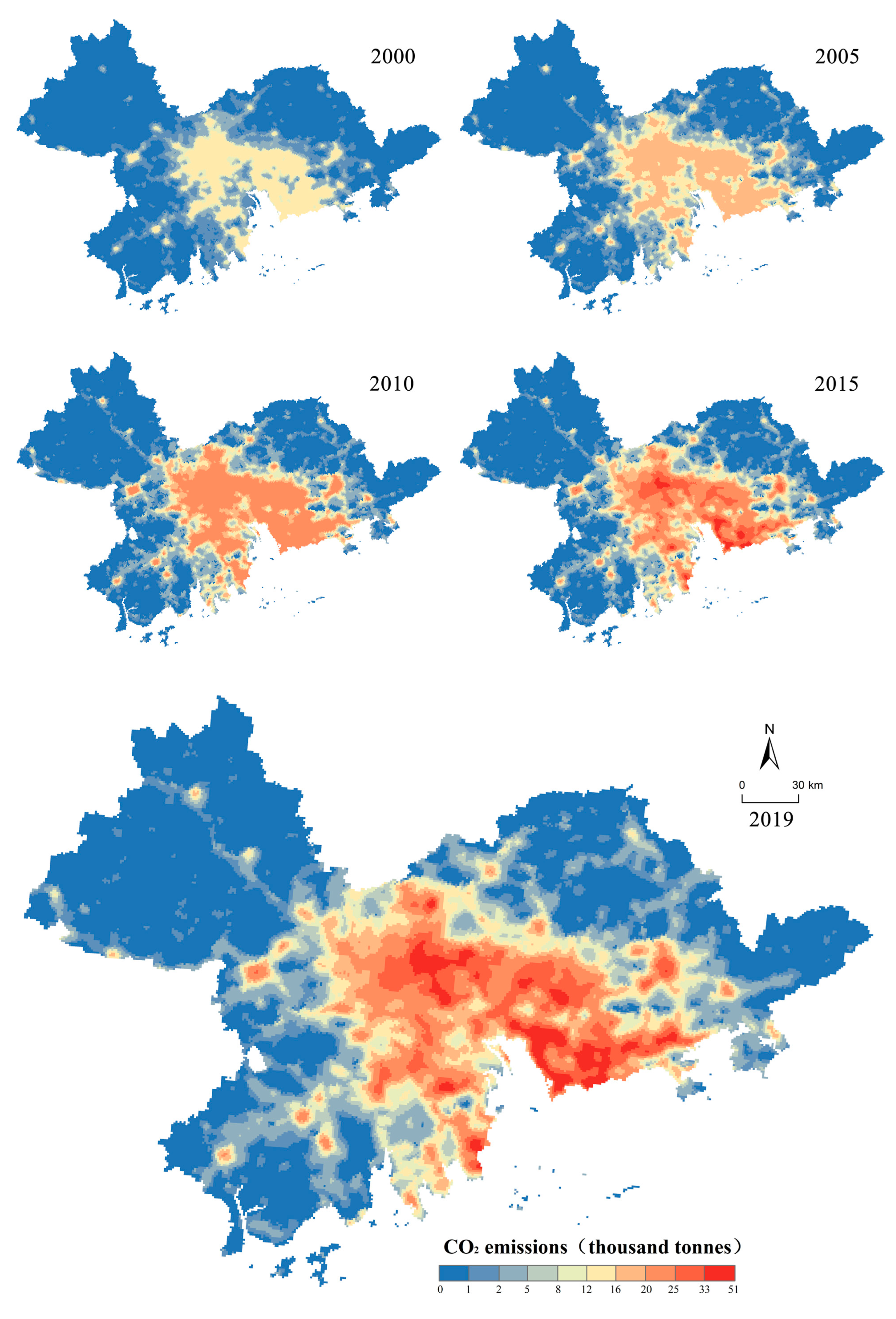
From 2000 to 2019, the total carbon emissions of these urban agglomerations exhibited a consistent upward trajectory, with carbon emissions primarily concentrated in the vicinity of the Pearl River estuary and gradually expanding outward. The eastern bank of the Pearl River demonstrated significantly higher levels of carbon emissions compared to its western counterpart, while the ecological barrier area outside the Pearl River Delta displayed considerably lower emissions than those observed around the estuary (Figure 2). During this period, Guangzhou, Foshan, Dongguan, Shenzhen, and other cities experienced rapid development in their early industrial enterprises, resulting in relatively high overall carbon emissions for these cities. Similarly, Huizhou, Zhongshan, Jiangmen, Zhaoqing, and Zhuhai also witnessed substantial growth due to their rapid industrial development stage; however, their total emission levels remained comparatively lower than those recorded by other cities.

3.1.3. Evolution of City-Scale Carbon Emission Patterns in the Pearl River Delta Urban Agglomeration

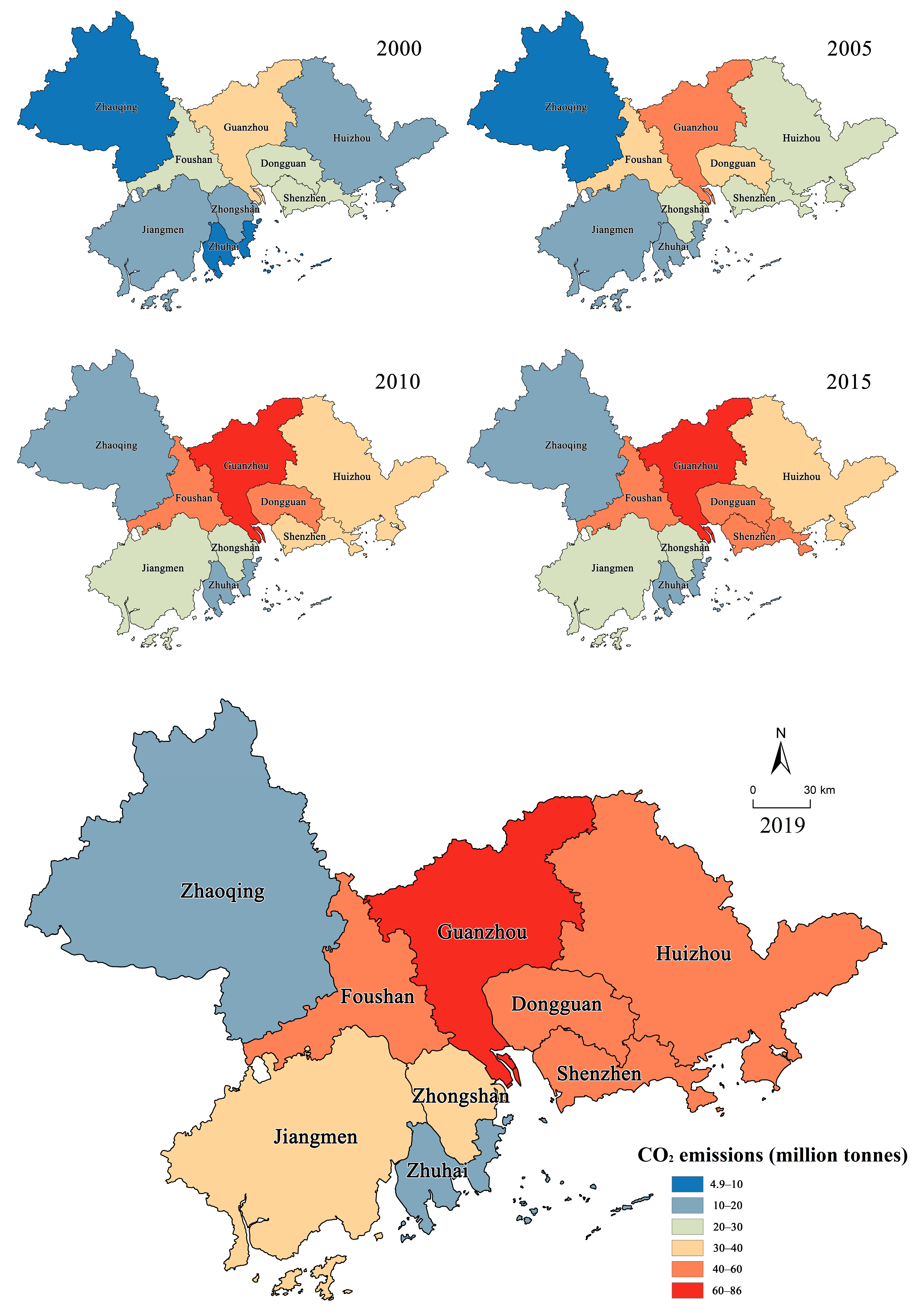
The carbon emissions of various cities within these urban agglomerations were computed based on spatial findings, as illustrated in Figure 3. Predominantly concentrated around the Pearl River Estuary, the carbon emissions within these urban agglomerations are primarily attributed to Guangzhou, consistently accounting for the largest proportion from 2000 to 2019 at approximately 20%. Foshan, Dongguan, and Shenzhen emerged as significant contributors to carbon emissions, while Huizhou, Jiangmen, and Zhongshan experienced rapid growth in their emission levels. Conversely, Zhuhai and Zhaoqing exhibited relatively lower levels of carbon emissions. (1) In 2000, the carbon emissions of this urban agglomeration accounted for 77% of the total carbon emissions in the Guangdong province. Guangzhou, Dongguan, and Foshan emerged as major contributors to carbon emissions, with shares of 20.67%, 19.31%, and 16.46%, respectively, within this urban agglomeration, while Zhaoqing and Zhuhai exhibited relatively lower levels of carbon emissions. (2) In 2005, the Pearl River Delta emerged as a prominent gateway for international trade and witnessed remarkable growth of numerous enterprises, characterized by high energy consumption. The carbon emission levels in the Pearl River Delta escalated from 151 million tons in 2000 to 239 million tons in 2005. Amongst these emissions, Guangzhou, Dongguan, and Foshan accounted for the largest shares, at 21.21%, 16.04%, and 15.95%, respectively, while Zhaoqing and Zhuhai exhibited comparatively lower carbon emission levels. During the period between 2000 and 2005, Huizhou and Zhaoqing experienced the most rapid increase in carbon emissions, with average annual growth rates of approximately 18.09% and 14.18%, respectively. As a consequence of implementing the dual-transfer policy initially proposed in 2004, which aimed to gradually relocate labor-intensive industries dispersed throughout the Pearl River Delta towards eastern/western regions as well as mountainous areas within Northern Guangdong Province, there was an expansion of Guangdong’s overall carbon emissions beyond just those originating from within the Pearl River Delta, thus leading to a decrease in total carbon emissions within this urban agglomeration province-wide. (3) In 2010, the carbon emissions of this urban agglomeration increased to 336 million tons. Guangzhou, Foshan, and Dongguan remained as the three cities with the highest carbon emissions in the Pearl River Delta, accounting for 21.19%, 16.03%, and 15.31% of regional carbon emissions, respectively. Zhuhai and Zhaoqing had the lowest carbon emissions, at 0.15 million tons and 16 million tons, respectively, in 2010. The cities experiencing the most rapid growth in carbon emissions over the past five years were Zhaoqing, Zhuhai, and Huizhou, which saw increases by factors of approximately 1.60, 1.50, and 1.47, respectively. (4) In 2015, the carbon emissions of this urban agglomeration reached a total of 354 million tons. As a result of the implementation of national carbon control measures in 2014, there was only a marginal increase compared to the 336 million tons recorded in 2010. Guangzhou, Foshan, and Dongguan are identified as the three cities with the highest carbon emissions, accounting for approximately 21.65%, 15.12%, and 14.76% of the overall regional carbon emissions, respectively. The growth rate of carbon emissions across all cities was relatively slow, while collectively contributing to about 70.74% of the province’s total carbon emission. (5) In 2019, the carbon emissions of this urban agglomeration rose to 400 million tons, with Guangzhou, Dongguan, and Foshan remaining as the primary contributors, accounting for 21.48%, 14.51%, and 13.81% of the total regional carbon emissions, respectively. Zhongshan, Huizhou, and Zhaoqing experienced significant growth in carbon emissions at average annual rates of 4.44%, 4.25%, and 4.11%, respectively.

3.1.4. Spatial Pattern Analysis of Carbon Emissions at the County Level in the Pearl River Delta Urban Agglomeration

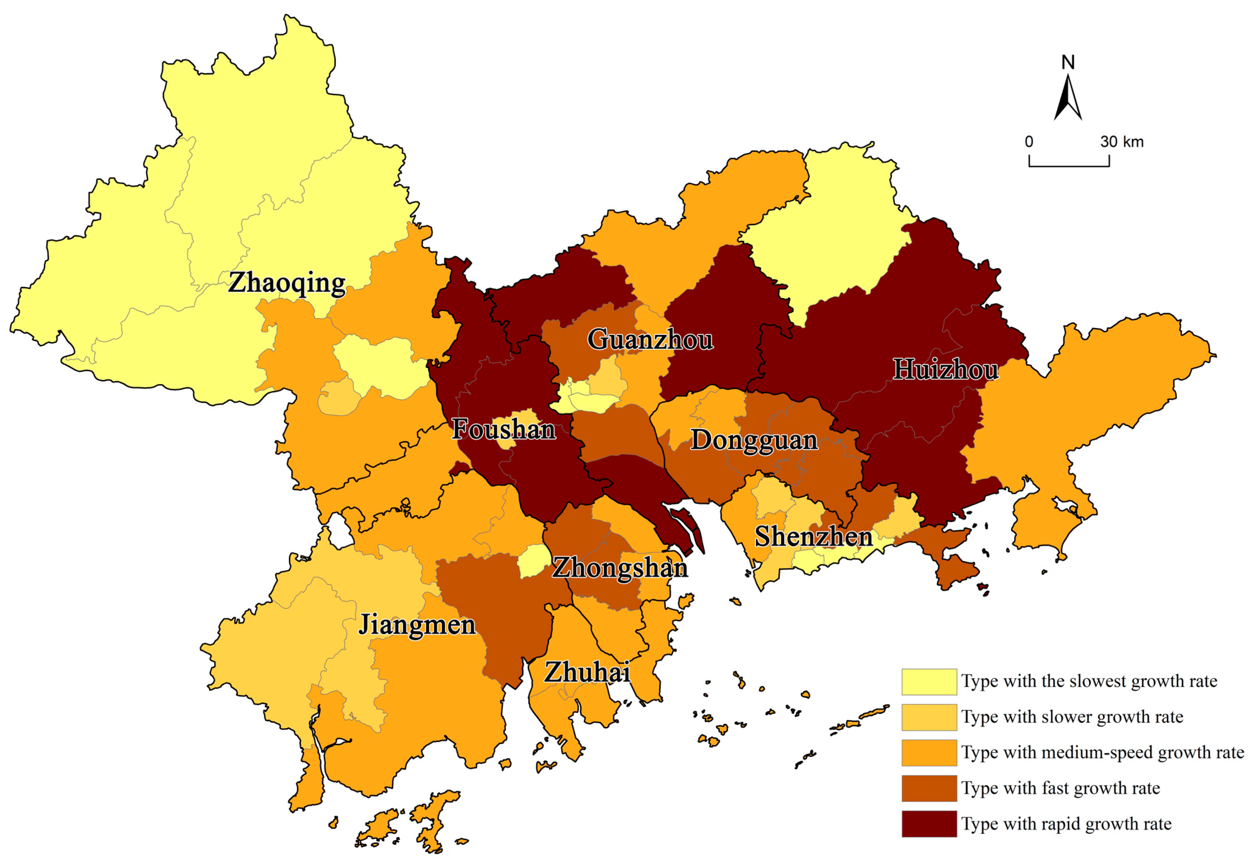
This paper employs a trend analysis to examine the temporal variation characteristics of carbon emissions in various districts and counties. Specifically, we calculate the SLOPE of carbon emissions from 2000 to 2019 using this method, and we apply ArcGIS software’s natural break point grading method (Jenks) to classify each county’s carbon emission change trend into five types: the type with the slowest growth rate, the type with a slower growth rate, the type with a medium-speed growth rate, the type with a fast growth rate, and the type with a rapid growth rate. To further analyze this slowdown phenomenon in urban agglomerations within the Pearl River Delta region after 2010, we separately calculated inclination values for carbon emissions during two periods (2000–2010 and 2010–2019) for each county. The results are presented in Figure 4 and Figure 5.

From 2000 to 2010, owing to the rapid development of the Pearl River Delta, carbon emissions witnessed a substantial increase in most districts and counties of Guangzhou, Foshan, Huizhou, and other cities. The western bank of the Pearl River experienced a moderate growth rate in carbon emissions, while the northern region of Zhaoqing displayed a relatively sluggish growth trend. From 2010 to 2019, as industrial transformation and upgrading continued to progress in the Pearl River Delta, there was a deceleration in the growth rate of carbon emissions around the Pearl River Estuary. Notably, Shunde District in Foshan, Southern Group in Zhongshan, Yantian District in Shenzhen, and Duanzhou District in Zhaoqing exhibited a downward trajectory for carbon emissions. Conversely, the western bank of the Pearl River demonstrated a comparatively slower growth trend with an expanding area experiencing rapid growth of carbon emissions. This phenomenon primarily manifested itself within certain districts and counties on both banks of the river; for instance, Jiangmen and Zhuhai showcased an accelerated growth trend (

Table 1. Types of carbon emission growth in Pearl River Delta urban agglomeration by stage.

Growth Type	During 2000–2010	During 2010–2019
Decreasing growth rate		Yantian District, Duanzhou District, Shunde District, Southern Group in Zhongshan
		Mean value of the SLOPEs is −0.0211
Slowest growth rate	Futian District, Longmen County, Haizhu District, Dinghu District, Yantian District, Liwan District, Yuexiu District, Luohu District, Jianghai District, Guangning County, Huaiji County, Fengkai County, Deqing County	Jianghai District, Guangning County, Huaiji County, Fengkai County, Deqing County, Huadu District, Sanshui District, Northeast Group in Zhongshan, Eastern Group in Zhongshan, Chancheng District, Gaoming District, Pengjiang District, Pengjiang District, Nanhai District, Northwest Group in Zhongshan, Southeast Area in Dongguan, Sihui City
	Mean SLOPE value = 0.0701	Mean SLOPE value = 0.0193
Slower growth rate	Tianhe District, Nanshan District, Pingshan District, Enping City, Duanzhou District, Kaiping City, Guangming District, Longhua District, Chancheng District	Liwan District, Yuexiu District, Luohu District, Nansha District, Kaiping City, Heshan City, Central Group in Zhongshan, Eastern Industrial Park Area in Dongguan, Water Township New Town Area in Dongguan, Doumen District
	Mean SLOPE value = 0.1601	Mean SLOPE value = 0.0581
Medium growth rate	Urban area in Dongguan, Conghua District, Jinwan District, Gaoyao District, Bao’an District, Southern Group in Zhongshan, Heshan City, Water Township New Town Area in Dongguan, Doumen District, Huangpu District, Xiangzhou District, Taishan City, Huidong County, Northeast Group in Zhongshan, Eastern Group in Zhongshan, Gaoming District, Pengjiang District, Sihui City	Futian District, Longmen County, Boluo County, Haizhu District, Tianhe District, Nanshan District, Pingshan District, Enping City, Dinghu District, Urban Area in Dongguan, Conghua District, Jinwan District, Gaoyao District
	Mean SLOPE value = 0.3176	Mean SLOPE value = 0.1022
Fast growth rate	Longgang District, Central Group in Zhongshan, Eastern Industrial Park Area in Dongguan, Songshan Lake Area in Dongguan, Baiyun District, Panyu District, Xinhui District, Northwest Group in Zhongshan, Southeast Area in Dongguan	Binhai Area, Songshan Lake Area in Dongguan, Baiyun District, Huangpu District, Panyu District, Zengcheng District, Xinhui District, Guangming District, Huicheng District, Longhua District, Xiangzhou District, Taishan City, Huidong County
	Mean SLOPE value = 0.4888	Mean SLOPE value = 0.1925
Rapid growth rate	Boluo County, Huiyang District, Shunde District, Nansha District, Zengcheng District, Huicheng District, Huadu District, Sanshui District, Nanhai District	Baoan District, Longgang District, Huiyang District
	Mean SLOPE value = 0.7873	Mean SLOPE value = 0.3671

).

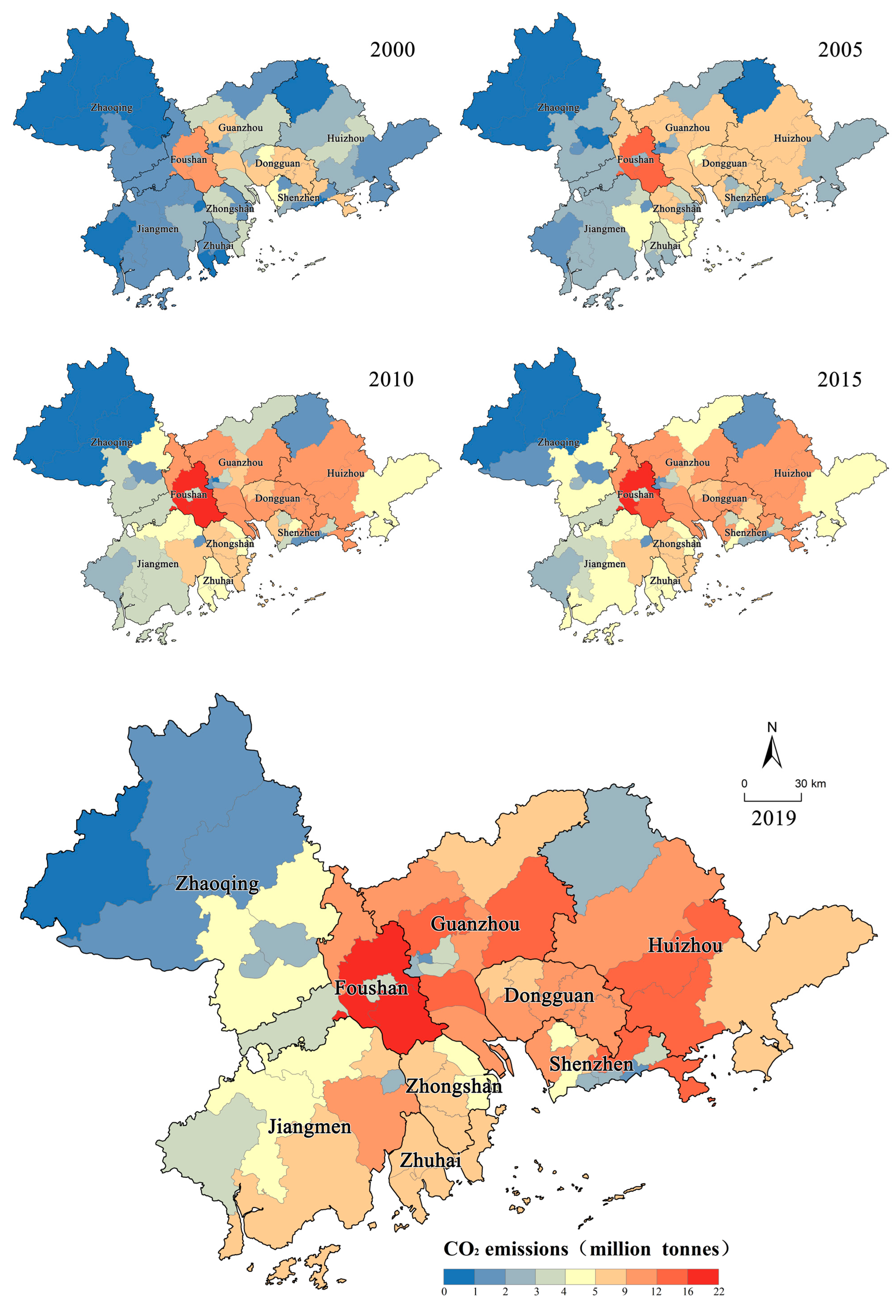
Based on the spatial analysis of carbon emissions, the county-level carbon emissions of this urban agglomerations were calculated and presented in Figure 6. Being the most economically developed region in Guangdong Province, this urban agglomeration experienced a rapid increase in carbon emissions, with high-value areas primarily concentrated around the Pearl River Estuary. Foshan Nanhai District, Shunde District, Huizhou Huiyang District, Huicheng district, Shenzhen Longgang District, Guangzhou Baiyun District, Panyu District, and Zengcheng District exhibited significant levels of carbon emissions, exceeding 12 million tons in 2019. Additionally, Dongguan and Huizhou also demonstrated substantial carbon emissions. Notably, the east bank of the Pearl River displayed significantly higher carbon emission levels compared to its western counterpart, while most districts and counties in Guangzhou, Dongguan, Huizhou, and Shenzhen witnessed a rapid increase in their respective carbon emissions. Conversely, Jiangmen, Zhuhai, and Zhaoqing, on the west bank of the Pearl River, had relatively low carbon emissions. Foshan Nanhai district and Shunde district stood out as the two regions with the highest carbon emissions in the Pearl River Delta.

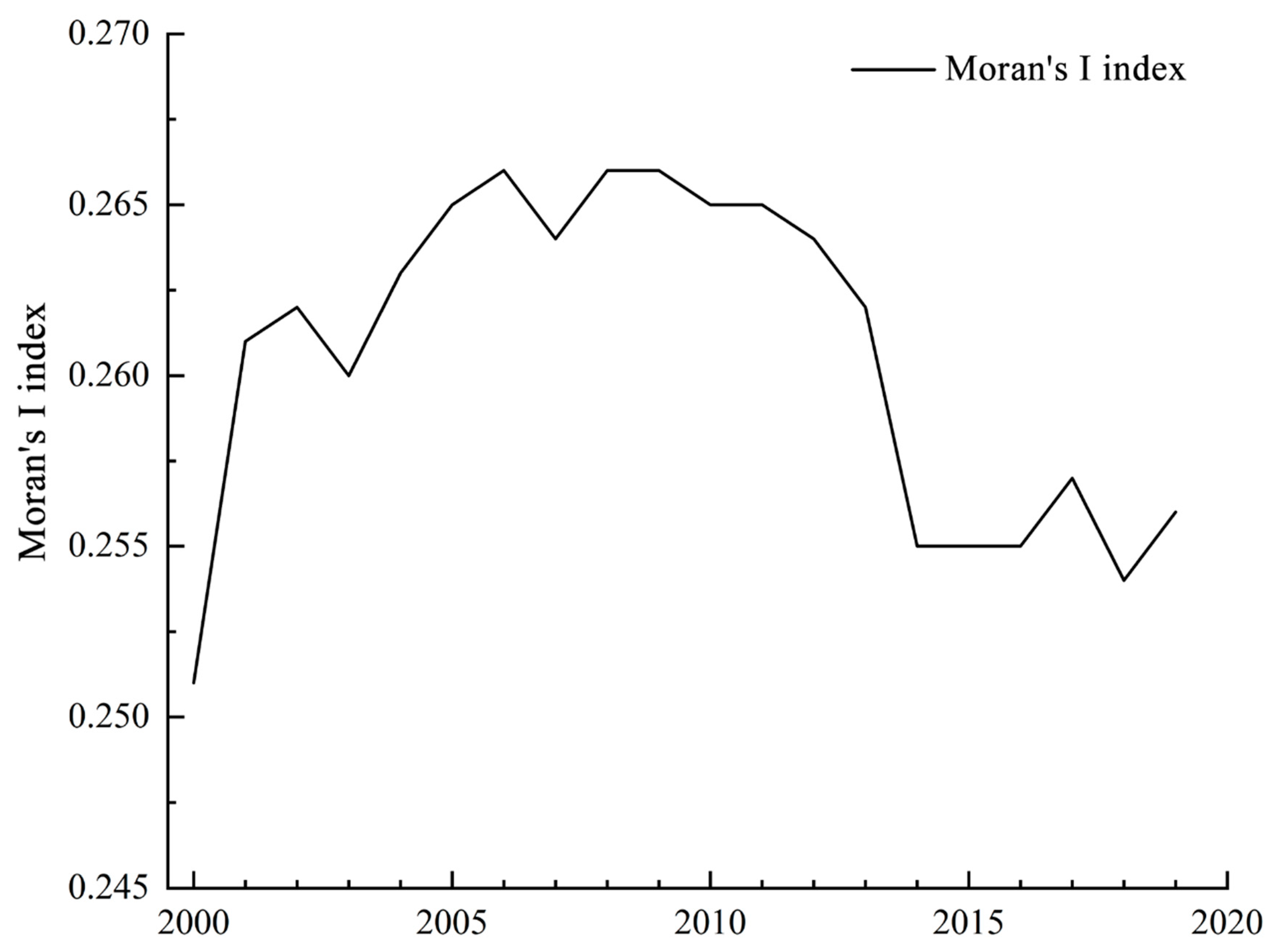
This study utilizes the Global Moran’s I analysis tool provided by GeoDa 1.22 software to compute the global Moran’s I index for carbon emissions at the county level in this urban agglomeration from 2000 to 2019. The findings are presented in Figure 7. The global Moran’s I index for county-scale carbon emissions in Pearl River Delta exhibits positive values, and their Z-values pass the significance test. Throughout the study period, districts and counties demonstrate significant spatial autocorrelation characteristics regarding carbon emissions, indicating that areas with higher (lower) carbon emissions tend to be surrounded by other areas with higher (lower) levels as well. From 2000 to 2014, the Moran’s I index for carbon emissions in this urban agglomerate followed an inverted U-shaped trend and stabilized after 2014. The degree of spatial concentration of carbon emissions within each district and county experienced an initial increase followed by a gradual decrease. After 2014, due to national efforts towards carbon control promotion and industrial transformation/upgrading initiatives targeting high-carbon emission regions, there was a tendency towards greater consistency in terms of carbon emission levels within this area.

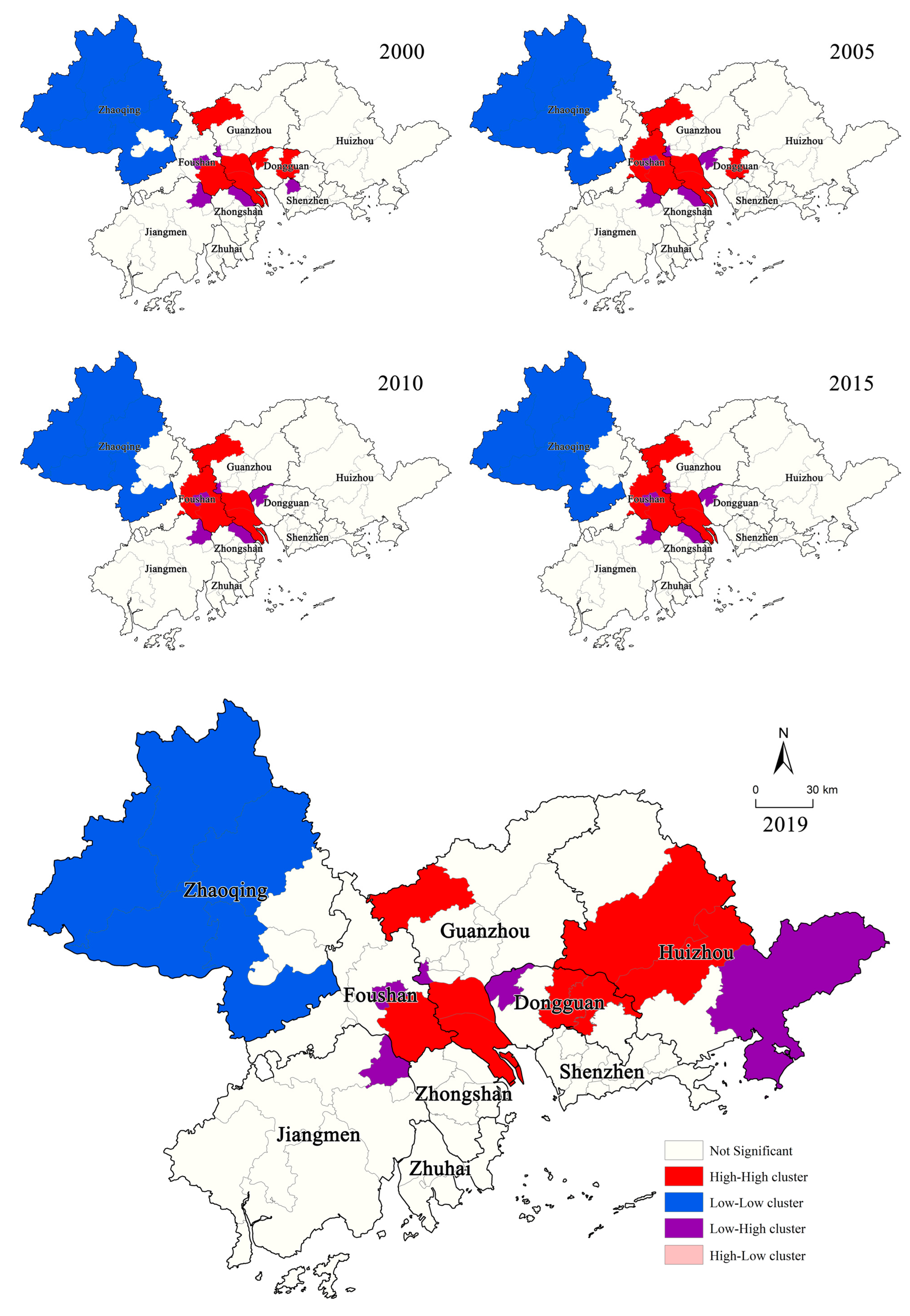
In order to further investigate the local spatial correlation of carbon emissions in this urban agglomeration at the regional and county levels, GeoDa and ArcGIS software were utilized to generate Local Moran’s I spatial distribution maps for carbon emissions in 2000, 2005, 2010, 2015, and 2019. According to Equations (3)–(5), the Local Moran’s I index was calculated to analyze the spatial variations between each region and its surrounding areas. The positive value of Local Moran’s I index indicates the presence of either high–high or low–low clustering, while the negative value suggests the presence of either high–low or low–high clustering. The results are presented in Figure 8. Overall, there are distinct agglomeration characteristics observed in carbon emissions at the county level within this urban agglomeration. These characteristics can be categorized as high–high concentration regions and low–low concentration regions. The high–high concentration regions primarily exist around the estuary of the Pearl River, where development zones are optimized for industrial production and daily life activities that require significant energy consumption resulting in large carbon emissions. Moreover, these high–high concentration areas exhibit an eastward diffusion trend, with Huizhou having the majority of districts and counties showing high–high concentrations. Low–low-concentration areas mainly surround the periphery of these high–high concentrated areas, while most districts and counties in Zhaoqing demonstrate consistently low–low concentrations. Due to accelerated construction efforts towards an ecological industry system in Zhaoqing, the number of districts and counties with consistently low concentrations has remained stable. In summary, there is a decreasing spatial disparity observed regarding carbon emissions within Pearl River Delta.

3.2. Driving Mechanisms of Carbon Emissions in the Pearl River Delta Urban Agglomeration

Based on regional characteristics and data availability, this study has selected indicators to analyze the driving mechanisms of carbon emissions in the Pearl River Delta. The total carbon emissions of the counties within this urban agglomeration in 2010, 2015, and 2019 were chosen as independent variables. Additionally, nine indicators representing seven factors at the county scale corresponding to these years were selected as explanatory factors and dependent variables (

Table 2. Description of indicators.

Factors	Variables	Variable Interpretation Instructions
Population urbanization	Urbanization (UPOP)	Size of permanent urban population in each district and county (unit: 10,000)
Economic development	Economic density (DGDP)	The ratio of GDP of each district and county to each district and county area (unit: yuan/km2)
Economic globalization	Foreign direct investment (FDI)	The actual amount of foreign direct investment used in each district and county (unit: 10,000 USD)
	Foreign trade (TEXIM)	Total amount of import and export trade of each district and county (unit: 100 million CNY)
Land use	Construction land (UAREA)	Total area of construction land in each district and county (unit: km2)
	Road density (DROAD)	The ratio of the total mileage of the road network of each district and county to the area of the district and county (unit: km/km2)
Household consumption	Total retail sales of consumer goods (TRSCG)	Total retail sales of consumer goods per capita in each district or county (unit: CNY/person)
Investment in fixed assets	Investment in fixed assets (FAI)	Investment in fixed assets of each district or county (unit: 10,000 CNY)
Government expenditure	Local government expenditure (GPBE)	Local government expenditure of each district or county (unit: 10,000 CNY)

). Geodetector was adopted to elucidate the influencing factors of county-level carbon emissions.

3.2.1. Single-Factor Detection Results

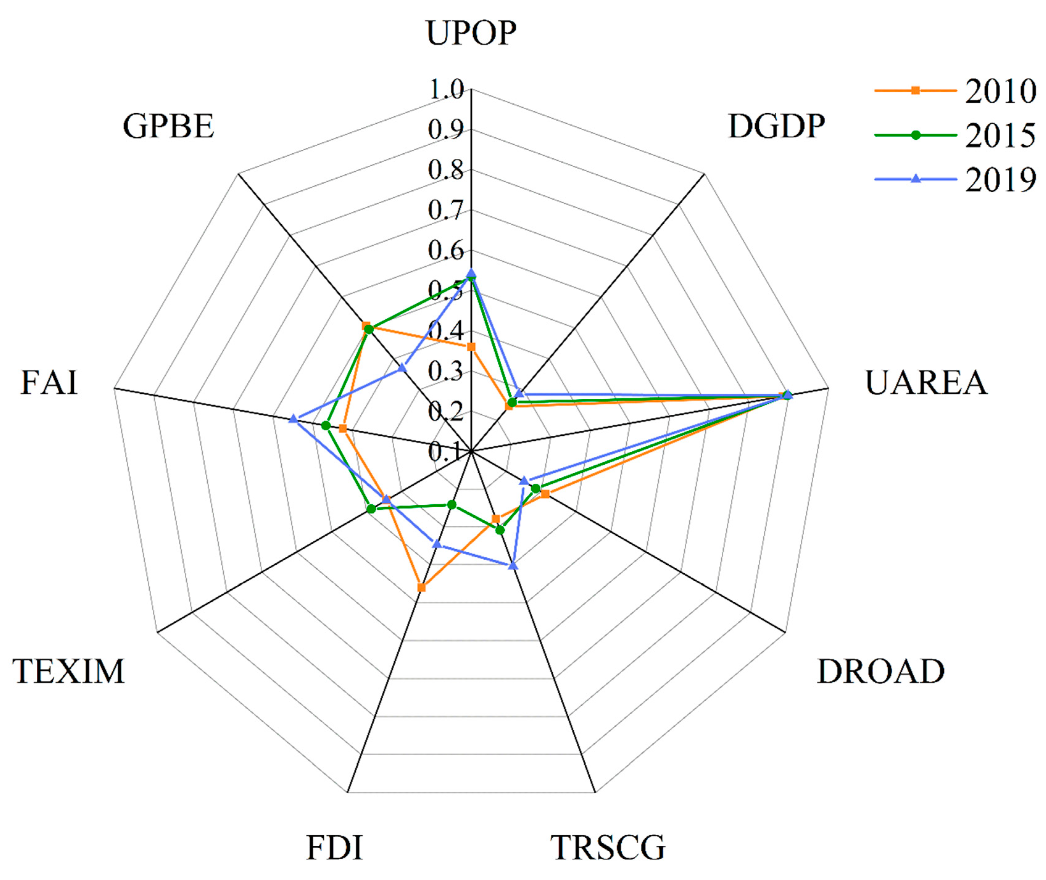
The driving factors contributing to spatial differentiation of carbon emissions in this urban agglomeration were identified using geographic detectors. According to Equations (6)–(8), the q value of each factor was calculated. A larger q value indicated that the factor explained more of the change in county-level carbon emissions. The results of single factor detection are presented in

Table 3. Explanatory power of each driving factor in different years.

Variables	Explanatory Power (q Value)
	2010	2015	2019
UPOP	0.359 ***	0.533 ***	0.541 ***
DGDP	0.245 ***	0.259 ***	0.284 ***
UAREA	0.886 ***	0.896 ***	0.898 ***
DROAD	0.313 ***	0.285 ***	0.252 **
TRSCG	0.279 *	0.309 ***	0.404 ***
FDI	0.461 ***	0.241 *	0.348 **
TEXIM	0.343 ***	0.386 ***	0.343 **
FAI	0.423 ***	0.466 ***	0.548 ***
GPBE	0.506 ***	0.495 ***	0.368 ***

Note: The significance levels for ***, **, and * are 0.01, 0.05, and 0.1, respectively, indicating statistical significance.

and Figure 9.

The explanatory power of factors in descending order in 2010, as presented in Table 3 and Figure 9, was observed to be construction land > local government expenditure > foreign direct investment > investment in fixed assets > urbanization > foreign trade > road density > household consumption > economic density. In 2015, the descending order of explanatory power shifted to construction land > urbanization > local government expenditure > investment in fixed assets > foreign trade > household consumption > road density > economic density > foreign direct investment. Similarly, in 2019, the descending order of explanatory power was found to be construction land > investment in fixed assets > urbanization > household consumption > local government expenditure > foreign direct investment > foreign trade > economic density > road density. Throughout the study period, it is noteworthy that construction land (UAREA) consistently exhibited the highest influence, and its explanatory power increased progressively over time. Other factors demonstrated varying changes in their respective explanatory powers. For instance, indicators such as investment in fixed assets, urbanization, household consumption, and economic density displayed significant increases during all three study periods, while indicators like foreign direct investment, road density, and local government expenditure experienced a decline.

The land use indicator exerted a significant influence on the spatial differentiation of carbon emissions in this urban agglomeration. Throughout the study period, construction land consistently demonstrated the highest explanatory power, with its q value progressively increasing from 0.886 in 2010 to 0.898 in 2019. On the one hand, the expansion of urban construction land caters to the demands of economic growth and urbanization within this urban agglomeration. However, it also engenders substantial energy consumption and carbon emissions. From 2010 to 2019, there was a rapid expansion in construction land area within this urban agglomeration, particularly between 2010 and 2015 when this expansion was most pronounced. Consequently, there was a significant increase in explanatory power observed in 2015 compared to that of 2010; subsequently, although there was a slight deceleration in the growth rate for construction land areas from 2015 to 2019, the explanatory power continued to exhibit marginal improvement.

The indicator representing population urbanization exerted a significant influence on the spatial differentiation of carbon emissions in the Pearl River Delta, with their explanatory power significantly enhanced over the study period. The explanatory power of urbanization increased from 0.359 in 2010 to 0.541 in 2019. The rapid development of the Pearl River Delta facilitated an elevation in its level of urbanization, attracting a substantial influx of labor forces and resulting in a concentration effect on population. The permanent population of the Pearl River Delta surged from 56.315 million in 2010 to 65.648 million in 2019, while its level of urbanization rose from 73.1% to 85.5%. The heightened consumption demand stemming from urbanization and population concentration drive an increase in energy consumption requirements, which profoundly impacts carbon emissions within the urban agglomeration.

3.2.2. Multifactor Interaction Detection Results

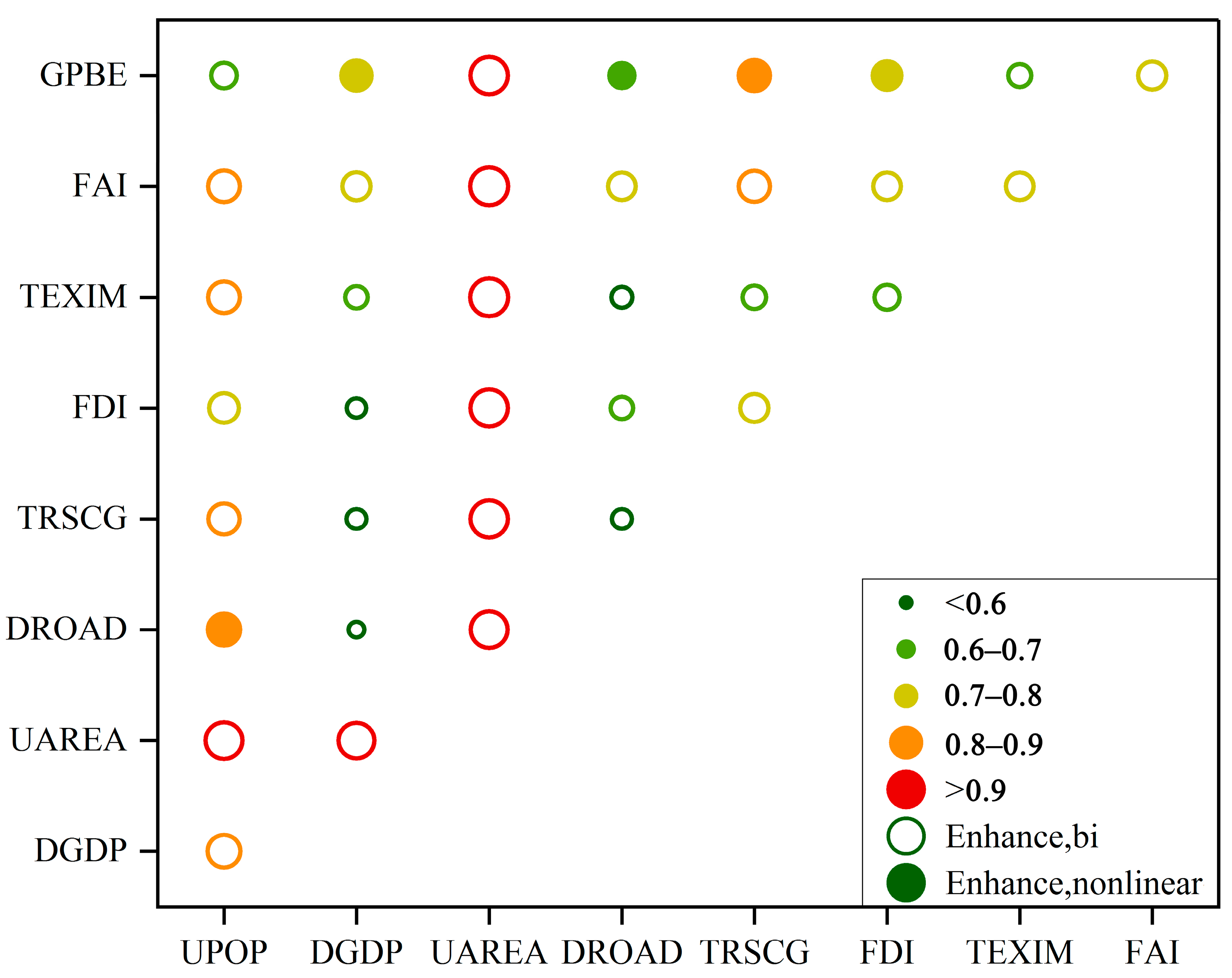
After examining the individual impact of each factor on the spatial variation of carbon emissions in this urban agglomeration, an analysis was conducted to explore the influence of multifactor interactions, as depicted in Figure 10, Figure 11 and Figure 12.

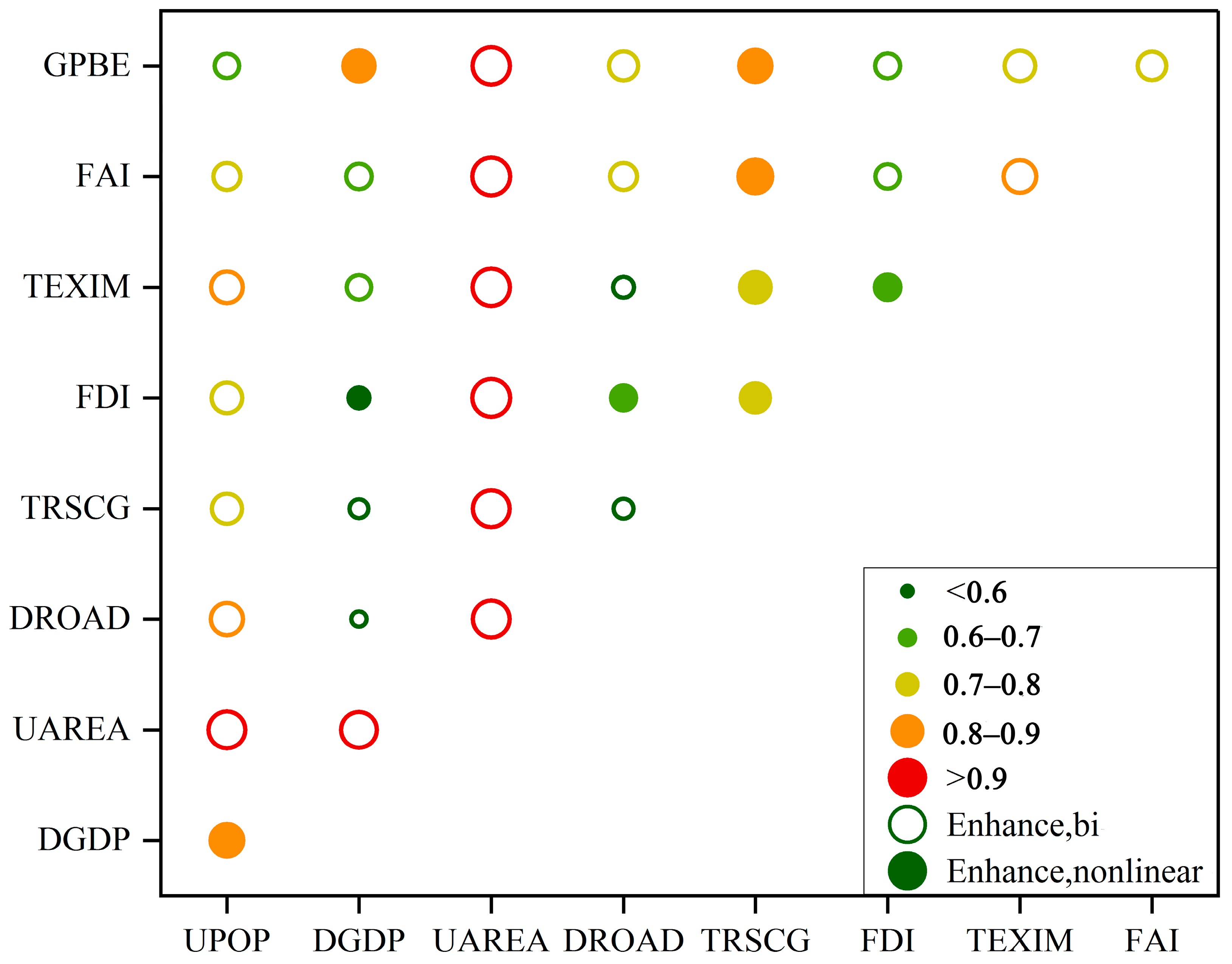
The influence of all factors on the spatial differentiation of carbon emissions significantly increased under interaction. Due to the robust detection and explanatory power of construction land (UAREA) as a single factor, the explanatory power of all other factors substantially improved after interacting with UAREA, reaching over 0.9. The interaction between other factors was also strong, enhancing the influence of low-explanatory-power factors detected via single-factor analysis. In 2010, household consumption and economic density had low single-factor detection influences of 0.279 and 0.245 respectively. However, their explanatory powers exceeded 0.7 when interacting with investment in fixed assets and local government expenditure (Figure 10). In 2015, economic density and foreign direct investment had low single-factor explanatory power, with q values of 0.259 and 0.241, respectively. However, after interacting with urbanization and local government expenditure, their explanatory powers reached approximately 0.8 (Figure 11). In 2019, local government expenditure, which initially had weak explanatory power, surpassed 0.7 under the interaction of factors such as urbanization, investment in fixed asset, and local government expenditure (Figure 12).

The explanatory power of land use and population urbanization indicators on carbon emissions exhibits a high degree of spatial differentiation across all study periods, particularly in 2015 and 2019. Notably, when interacting with economic density, the explanatory power is significantly enhanced. These findings highlight the close relationship between population urbanization, economic growth, and land use patterns in the Pearl River Delta regarding carbon emissions’ spatial distribution. The rapid economic development within this urban agglomeration has been accompanied by steady progress in the urbanization process, leading to increased population concentration and continuous expansion of urban construction land. Consequently, domestic energy demand has surged alongside high levels of energy consumption for both production and lifestyle purposes, resulting in substantial carbon emissions. Additionally, indicators representing investment in fixed assets and local government expenditure exhibit strong interactions with most influencing factors. Furthermore, foreign trade demonstrates intertwined relationships with indicators related to population urbanization, land use patterns, and household consumption. As the process of urbanization deepens continuously while opportunities within the Pearl River Delta progress further; infrastructure improvements have been witnessed alongside enhancements in household consumption, providing favorable conditions for foreign trade activities to thrive. This increase in foreign trade scale has subsequently attracted a significant influx of production factors while accelerating the pace of urbanization.

4. Conclusions

The PSO-BP algorithm, integrated with multi-source data including remote sensing, population, and economy, was employed in this study to construct a multi-scale and multi-level spatial database of carbon emissions in this urban agglomeration. This enabled the transformation of carbon emission spatial distributions from administrative boundaries to kilometer grids and facilitated the accurate implementation of the “dual carbon” target. Trend analysis and exploratory spatial data analysis (ESDA) were utilized to systematically examine the spatiotemporal characteristics of carbon emissions at the city and county levels from 2000 to 2019. The spatiotemporal dynamics of carbon emissions in this urban agglomeration were analyzed at the city, district, and county levels. Furthermore, a comprehensive framework for analyzing multiple influencing factors such as urbanization, economic growth, land use, household consumption, foreign trade, fixed asset investment, and government expenditure was established to promote understanding of the county-level driving mechanisms behind carbon emissions.

Carbon emissions in this region exhibit distinct spatial patterns, characterized by high–high and low–low concentrations. Carbon emissions were predominantly concentrated in the counties surrounding the Pearl River Estuary, with significantly higher emission levels observed in counties on the eastern bank of the Pearl River compared to those on the western bank. Overall, there was a partial reduction in spatial disparities regarding carbon emissions.

In 2010, 2015, and 2019, construction land consistently emerged as the most influential factor, with its explanatory power progressively increasing over time. The explanatory power of other factors varied with their changing dynamics. The interaction effect significantly amplified the effect of various factors on the spatial differentiation of county level carbon emissions, particularly enhancing the impact of low-explanatory-power single factors.

With the continuous economic and social development of the Pearl River Delta urban agglomeration, construction land expansion significantly influences the county-level carbon emissions of this region. Moreover, the escalating demand for land to accommodate high-carbon projects will inevitably result in substantial carbon emissions. Therefore, local governments should rigorously regulate land requirements for high-carbon projects such as thermal power plants and refining and chemical plants while concurrently enhancing spatial utilization efficiency for industrial land and energy infrastructure with high carbon footprints. Additionally, local governments should bolster investments in clean energy initiatives and advancements in energy-saving and emission-reduction technologies. This includes improving the energy efficiency of transportation systems, buildings, water supply networks, and power supply facilities to curtail both energy consumption levels and associated carbon emissions.

5. Discussion

In this research, a spatial simulation of carbon emissions based on multi-source data was conducted with the support of PSO-BP. The focus of this study was to investigate the spatiotemporal dynamics and driving mechanisms of carbon emissions in this urban agglomeration at both district and county levels. The aim was to provide a decision-making basis and reference for the low-carbon development path not only for this urban agglomeration but also for other urban agglomerations. However, this research still has following shortcomings:

(1)

The spatial simulation of carbon emissions primarily relies on a top-down approach. Despite the coupling of high-precision population and economic spatial data, there is still room for further improvement in the spatial accuracy of carbon emissions data. In future studies, it is recommended to consider incorporating a combination of bottom-up and top-down approaches to enhance the integration of multi-source POI data, big data from industrial enterprises, high-precision land use data, etc., thereby enhancing the accuracy of spatial simulations for carbon emissions.

(2)

Energy consumption, energy structure, and other factors directly impact carbon emissions. However, obtaining data on energy consumption is challenging due to the varying statistical caliber at the city, district, and county levels. To enhance the accuracy of statistical accounting for carbon emissions in future research, it is recommended to conduct field surveys on energy consumption data at the district and county levels, as well as the enterprise and household levels.

(3)

The driving mechanisms of carbon emissions identified in this study primarily focused on the internal influencing factors of urban agglomerations. With the implementation of the new dual-cycle development pattern, there is increased connectivity between the internal and external aspects of urban agglomerations. Therefore, it is essential to enhance research on the impact of external influencing factors on local carbon emissions in urban agglomerations.

References

1. McNutt, M. Time’s up, CO2. Science 2019, 365, 411. [Google Scholar] [CrossRef] [PubMed]
2. Bulkeley, H. Governing climate change: The politics of risk society? Trans. Inst. Br. Geogr. 2001, 26, 430–447. [Google Scholar] [CrossRef]
3. Adger, W.N. Social Capital, Collective Action, and Adaptation to Climate Change. Econ. Geogr. 2003, 79, 387–404. [Google Scholar] [CrossRef]
4. Thomas, C.D.; Cameron, A.; Green, R.E.; Bakkenes, M.; Beaumont, L.J.; Collingham, Y.C.; Erasmus, B.F.N.; de Siqueira, M.F.; Grainger, A.; Hannah, L.; et al. Extinction risk from climate change. Nature 2004, 427, 145–148. [Google Scholar] [CrossRef] [PubMed]
5. Nordhaus, W.D. A Review of the Stern Review on the Economics of Climate Change. J. Econ. Lit. 2007, 45, 686–702. [Google Scholar] [CrossRef]
6. Meinshausen, M.; Lewis, J.; McGlade, C.; Gütschow, J.; Nicholls, Z.; Burdon, R.; Cozzi, L.; Hackmann, B. Realization of Paris Agreement pledges may limit warming just below 2 °C. Nature 2022, 604, 304–309. [Google Scholar] [CrossRef]
7. Roelfsema, M.; van Soest, H.L.; Harmsen, M.; van Vuuren, D.P.; Bertram, C.; den Elzen, M.; Höhne, N.; Iacobuta, G.; Krey, V.; Kriegler, E.; et al. Taking stock of national climate policies to evaluate implementation of the Paris Agreement. Nat. Commun. 2020, 11, 2096. [Google Scholar] [CrossRef]
8. Schneider, L.; Duan, M.; Stavins, R.; Kizzier, K.; Broekhoff, D.; Jotzo, F.; Winkler, H.; Lazarus, M.; Howard, A.; Hood, C. Double counting and the Paris Agreement rulebook. Science 2019, 366, 180–183. [Google Scholar] [CrossRef]
9. Rogelj, J.; Huppmann, D.; Krey, V.; Riahi, K.; Clarke, L.; Gidden, M.; Nicholls, Z.; Meinshausen, M. A new scenario logic for the Paris Agreement long-term temperature goal. Nature 2019, 573, 357–363. [Google Scholar] [CrossRef]
10. Tanaka, K.; O’Neill, B.C. The Paris Agreement zero-emissions goal is not always consistent with the 1.5 °C and 2 °C temperature targets. Nat. Clim. Chang. 2018, 8, 319–324. [Google Scholar] [CrossRef]
11. Acuto, M.; Parnell, S.; Seto, K.C. Building a global urban science. Nat. Sustain. 2018, 1, 2–4. [Google Scholar] [CrossRef]
12. Dhakal, S. Urban energy use and carbon emissions from cities in China and policy implications. Energy Policy 2009, 37, 4208–4219. [Google Scholar] [CrossRef]
13. Li, Z.; Wang, F.; Kang, T.; Wang, C.; Chen, X.; Miao, Z.; Zhang, L.; Ye, Y.; Zhang, H. Exploring differentiated impacts of socioeconomic factors and urban forms on city-level CO2 emissions in China: Spatial heterogeneity and varying importance levels. Sustain. Cities Soc. 2022, 84, 104028. [Google Scholar] [CrossRef]
14. Streets, D.G.; Jiang, K.; Hu, X.; Sinton, J.E.; Zhang, X.-Q.; Xu, D.; Jacobson, M.Z.; Hansen, J.E. Recent Reductions in China’s Greenhouse Gas Emissions. Science 2001, 294, 1835–1837. [Google Scholar] [CrossRef]
15. Chen, Y.; Wang, J.; Xu, L.; Ye, S. Spatio-temporal Variations and Influencing Factors of Energy Efficiency in Fujian Province. J. Fujian Norm. Univ. Nat. Sci. Ed. 2024, 40, 20–29. [Google Scholar]
16. Zhang, Q.; Lin, J.; Wang, Q.; Chen, D.; Zhou, T.; Dang, N.; Zhuang, X.; Li, Y.; Luo, D. The Impact of Main Functional Area Strategy on Regional Energy Consumption Carbon Emission: A Case Study of Fujian Province. J. Fujian Norm. Univ. Nat. Sci. Ed. 2024, 40, 30–43. [Google Scholar]
17. Qi, X.; Huang, R.; Jia, Y.; Huang, Q. Analysis of Spatial and Temporal Characteristics and Driving Factors of Carbon Emissions at the County Level in Coal Resource-Based Areas:Take Shanxi Province as an Example. J. North China Inst. Water Conserv. Hydroelectr. Power Soc. Sci. Ed. 2024, 40, 1–11. [Google Scholar] [CrossRef]
18. Elvidge, C.D.; Baugh, K.E.; Kihn, E.A.; Kroehl, H.W.; Davis, E.R.; Davis, C.W. Relation between satellite observed visible-near infrared emissions, population, economic activity and electric power consumption. Int. J. Remote Sens. 1997, 18, 1373–1379. [Google Scholar] [CrossRef]
19. Doll, C.N.H.; Muller, J.P.; Elvidge, C.D. Night-time imagery as a tool for global mapping of socioeconomic parameters and greenhouse gas emissions. Ambio 2000, 29, 157–162. [Google Scholar] [CrossRef]
20. Ghosh, T.; Elvidge, C.D.; Sutton, P.C.; Baugh, K.E.; Ziskin, D.; Tuttle, B.T. Creating a global grid of distributed fossil fuel CO2 emissions from nighttime satellite imagery. Energies 2010, 3, 1895–1913. [Google Scholar] [CrossRef]
21. Oda, T.; Maksyutov, S. A very high-resolution (1 km × 1 km) global fossil fuel CO2 emission inventory derived using a point source database and satellite observations of nighttime lights. Atmos. Chem. Phys. 2011, 11, 543–556. [Google Scholar] [CrossRef]
22. Su, Y.; Chen, X.; Li, Y.; Liao, J.; Ye, Y.; Zhang, H.; Huang, N.; Kuang, Y. China‘s 19-year city-level carbon emissions of energy consumptions, driving forces and regionalized mitigation guidelines. Renew. Sustain. Energy Rev. 2014, 35, 231–243. [Google Scholar] [CrossRef]
23. Shi, K.; Yu, B.; Huang, Y.; Hu, Y.; Yin, B.; Chen, Z.; Chen, L.; Wu, J. Evaluating the Ability of NPP-VIIRS Nighttime Light Data to Estimate the Gross Domestic Product and the Electric Power Consumption of China at Multiple Scales: A Comparison with DMSP-OLS Data. Remote Sens. 2014, 6, 1705–1724. [Google Scholar] [CrossRef]
24. Zhang, L.; Lei, J.; Wang, C.; Wang, F.; Geng, Z.; Zhou, X. Spatio-temporal variations and influencing factors of energy-related carbon emissions for Xinjiang cities in China based on time-series nighttime light data. J. Geogr. Sci. 2022, 32, 1886–1910. [Google Scholar] [CrossRef]
25. Chen, J.; Gao, M.; Cheng, S.; Hou, W.; Song, M.; Liu, X.; Liu, Y.; Shan, Y. County-level CO2 emissions and sequestration in China during 1997–2017. Sci. Data 2020, 7, 391. [Google Scholar] [CrossRef]
26. Chen, J.; Gao, M.; Cheng, S.; Liu, X.; Hou, W.; Song, M.; Li, D.; Fan, W. China’s city-level carbon emissions during 1992–2017 based on the inter-calibration of nighttime light data. Sci. Rep. 2021, 11, 3323. [Google Scholar] [CrossRef]
27. Zhu, N.; Li, X.; Yang, S.; Ding, Y.; Zeng, G. Spatio-temporal dynamics and influencing factors of carbon emissions (1997–2019) at county level in mainland China based on DMSP-OLS and NPP-VIIRS Nighttime Light Datasets. Heliyon 2024, 10, e37245. [Google Scholar] [CrossRef]
28. Xiang, C.; Mei, Y.; Liang, A. Analysis of Spatiotemporal Changes in Energy Consumption Carbon Emissions at District and County Levels Based on Nighttime Light Data—A Case Study of Jiangsu Province in China. Remote Sens. 2024, 16, 3514. [Google Scholar] [CrossRef]
29. Jiang, L.; Yang, L.; Wu, Q.; Zhang, X. How does extreme heat affect carbon emission intensity? Evidence from county-level data in China. Econ. Model. 2024, 139, 106814. [Google Scholar] [CrossRef]
30. Xie, Z.; Wang, L.; Zhao, R.; Xiao, L.; Ding, M.; Yao, S.; Chuai, X.; Rong, P. County-level carbon budget and carbon compensation in the Yellow River Basin: A perspective with balancing efficiency and equity. Environ. Dev. Sustain. 2024. [Google Scholar] [CrossRef]
31. Zhou, C.; Wang, S. Examining the determinants and the spatial nexus of city-level CO2 emissions in China: A dynamic spatial panel analysis of China’s cities. J. Clean. Prod. 2018, 171, 917–926. [Google Scholar] [CrossRef]
32. Ke, N.; Lu, X.; Kuang, B.; Zhang, X. Regional disparities and evolution trend of city-level carbon emission intensity in China. Sustain. Cities Soc. 2023, 88, 104288. [Google Scholar] [CrossRef]
33. Cheng, Y.; Wang, Z.; Ye, X.; Wei, Y.D. Spatiotemporal dynamics of carbon intensity from energy consumption in China. J. Geogr. Sci. 2014, 24, 631–650. [Google Scholar] [CrossRef]
34. York, R.; Rosa, E.A.; Dietz, T. STIRPAT, IPAT and ImPACT: Analytic tools for unpacking the driving forces of environmental impacts. Ecol. Econ. 2003, 46, 351–365. [Google Scholar] [CrossRef]
35. Brizga, J.; Feng, K.; Hubacek, K. Drivers of CO2 emissions in the former Soviet Union: A country level IPAT analysis from 1990 to 2010. Energy 2013, 59, 743–753. [Google Scholar] [CrossRef]
36. Wang, H.; Ang, B.W.; Su, B. Assessing drivers of economy-wide energy use and emissions: IDA versus SDA. Energy Policy 2017, 107, 585–599. [Google Scholar] [CrossRef]
37. Wang, C.; Wang, F.; Zhang, X.; Yang, Y.; Su, Y.; Ye, Y.; Zhang, H. Examining the driving factors of energy related carbon emissions using the extended STIRPAT model based on IPAT identity in Xinjiang. Renew. Sustain. Energy Rev. 2017, 67, 51–61. [Google Scholar] [CrossRef]
38. Wang, F.; Wang, C.; Chen, J.; Li, Z.; Li, L. Examining the determinants of energy-related carbon emissions in Central Asia: Country-level LMDI and EKC analysis during different phases. Environ. Dev. Sustain. 2020, 22, 7743–7769. [Google Scholar] [CrossRef]
39. Li, Z.; Chen, X.; Ye, Y.; Wang, F.; Liao, K.; Wang, C. The impact of digital economy on industrial carbon emission efficiency at the city level in China: Gravity movement trajectories and driving mechanisms. Environ. Technol. Innov. 2024, 33, 103511. [Google Scholar] [CrossRef]
40. Xu, L.; Du, H.; Zhang, X. Driving forces of carbon dioxide emissions in China’s cities: An empirical analysis based on the geodetector method. J. Clean. Prod. 2021, 287, 125169. [Google Scholar] [CrossRef]
41. Liao, K.; Huang, W.; Wang, C.; Wu, R.; Hu, Y. Spatio-Temporal Evolution Features and Impact Factors of Urban Expansion in Underdeveloped Cities: A Case Study of Nanchang, China. Land 2022, 11, 1799. [Google Scholar] [CrossRef]
42. Su, Y.; Wu, J.; Ciais, P.; Zheng, B.; Wang, Y.; Chen, X.; Li, X.; Li, Y.; Wang, Y.; Wang, C.; et al. Differential impacts of urbanization characteristics on city-level carbon emissions from passenger transport on road: Evidence from 360 cities in China. Build. Environ. 2022, 219, 109165. [Google Scholar] [CrossRef]
43. Liu, S.; Shen, J.; Liu, G.; Wu, Y.; Shi, K. Exploring the effect of urban spatial development pattern on carbon dioxide emissions in China: A socioeconomic density distribution approach based on remotely sensed nighttime light data. Comput. Environ. Urban Syst. 2022, 96, 101847. [Google Scholar] [CrossRef]
44. Wang, S.; Liu, X.; Zhou, C.; Hu, J.; Ou, J. Examining the impacts of socioeconomic factors, urban form, and transportation networks on CO2 emissions in China’s megacities. Appl. Energy 2017, 185, 189–200. [Google Scholar] [CrossRef]
45. Shi, K.; Xu, T.; Li, Y.; Chen, Z.; Gong, W.; Wu, J.; Yu, B. Effects of urban forms on CO2 emissions in China from a multi-perspective analysis. J. Environ. Manag. 2020, 262, 110300. [Google Scholar] [CrossRef]
46. Li, Y.; Lv, C.; Yang, N.; Liu, H.; Liu, Z. A study of high temporal-spatial resolution greenhouse gas emissions inventory for on-road vehicles based on traffic speed-flow model: A case of Beijing. J. Clean. Prod. 2020, 277, 122419. [Google Scholar] [CrossRef]
47. Duan, C.; Zhu, W.; Wang, S.; Chen, B. Drivers of global carbon emissions 1990–2014. J. Clean. Prod. 2022, 371, 133371. [Google Scholar] [CrossRef]
48. Khan, M.K.; Teng, J.-Z.; Khan, M.I.; Khan, M.O. Impact of globalization, economic factors and energy consumption on CO2 emissions in Pakistan. Sci Total Environ. 2019, 688, 424–436. [Google Scholar] [CrossRef]
49. Zhang, Y.; Zhang, S. The impacts of GDP, trade structure, exchange rate and FDI inflows on China’s carbon emissions. Energy Policy 2018, 120, 347–353. [Google Scholar] [CrossRef]
50. Lin, H.; Wang, X.; Bao, G.; Xiao, H. Heterogeneous Spatial Effects of FDI on CO2 Emissions in China. Earths Future 2022, 10, e2021EF002331. [Google Scholar] [CrossRef]
51. Hertwich, E.G. Increased carbon footprint of materials production driven by rise in investments. Nat. Geosci. 2021, 14, 151–155. [Google Scholar] [CrossRef]
52. Zhao, X.; Zhang, X.; Shao, S. Decoupling CO2 emissions and industrial growth in China over 1993–2013: The role of investment. Energy Econ. 2016, 60, 275–292. [Google Scholar] [CrossRef]
53. Cheng, S.; Chen, Y.; Meng, F.; Chen, J.; Liu, G.; Song, M. Impacts of local public expenditure on CO2 emissions in Chinese cities: A spatial cluster decomposition analysis. Resour. Conserv. Recycl. 2021, 164, 105217. [Google Scholar] [CrossRef]
54. Xu, C.; Xu, Y.; Chen, J.; Huang, S.; Zhou, B.; Song, M. Spatio-temporal efficiency of fiscal environmental expenditure in reducing CO2 emissions in China’s cities. J. Environ. Manag. 2023, 334, 117479. [Google Scholar] [CrossRef]
55. Wang, Q. Effects of urbanisation on energy consumption in China. Energy Policy 2014, 65, 332–339. [Google Scholar] [CrossRef]
56. Wu, S.; Lei, Y.; Li, S. CO2 emissions from household consumption at the provincial level and interprovincial transfer in China. J. Clean. Prod. 2019, 210, 93–104. [Google Scholar] [CrossRef]
57. Zhang, Z.; Zhao, Y.; Su, B.; Zhang, Y.; Wang, S.; Liu, Y.; Li, H. Embodied carbon in China’s foreign trade: An online SCI-E and SSCI based literature review. Renew. Sustain. Energy Rev. 2017, 68, 492–510. [Google Scholar] [CrossRef]
58. Zhang, X.; Zhao, Y. Identification of the driving factors’ influences on regional energy-related carbon emissions in China based on geographical detector method. Environ. Sci. Pollut. Res. 2018, 25, 9626–9635. [Google Scholar] [CrossRef]
59. Su, Y.; Chen, X.; Wang, C.; Zhang, H.; Liao, J.; Ye, Y.; Wang, C. A new method for extracting built-up urban areas using DMSP-OLS nighttime stable lights: A case study in the Pearl River Delta, southern China. GISci. Remote Sens. 2015, 52, 218–238. [Google Scholar] [CrossRef]
60. Chen, J.; Liu, J.; Qi, J.; Gao, M.; Cheng, S.; Li, K.; Xu, C. City- and county-level spatio-temporal energy consumption and efficiency datasets for China from 1997 to 2017. Sci. Data 2022, 9, 101. [Google Scholar] [CrossRef]
61. Shan, Y.; Guan, Y.; Hang, Y.; Zheng, H.; Li, Y.; Guan, D.; Li, J.; Zhou, Y.; Li, L.; Hubacek, K. City-level emission peak and drivers in China. Sci. Bull. 2022, 67, 1910–1920. [Google Scholar] [CrossRef] [PubMed]
62. Zhang, L.; Ruan, J.; Zhang, Z.; Qin, Z.; Lei, Z.; Cai, B.; Wang, S.; Tang, L. City-level pathways to carbon peak and neutrality in China. Cell Rep. Sustain. 2024, 1, 100102. [Google Scholar] [CrossRef]
63. Cai, B.; Liang, S.; Zhou, J.; Wang, J.; Cao, L.; Qu, S.; Xu, M.; Yang, Z. China high resolution emission database (CHRED) with point emission sources, gridded emission data, and supplementary socioeconomic data. Resour. Conserv. Recycl. 2018, 129, 232–239. [Google Scholar] [CrossRef]
64. Zhou, Y.; Li, K.; Liang, S.; Zeng, X.; Cai, Y.; Meng, J.; Shan, Y.; Guan, D.; Yang, Z. Trends, Drivers, and Mitigation of CO2 Emissions in the Guangdong–Hong Kong–Macao Greater Bay Area. Engineering 2023, 23, 138–148. [Google Scholar] [CrossRef]
65. Zhou, Y.; Shan, Y.; Liu, G.; Guan, D. Emissions and low-carbon development in Guangdong-Hong Kong-Macao Greater Bay Area cities and their surroundings. Appl. Energy 2018, 228, 1683–1692. [Google Scholar] [CrossRef]
66. Song, Y.; Ma, M.; Veroustraete, F. Comparison and conversion of AVHRR GIMMS and SPOT VEGETATION NDVI data in China. Int. J. Remote Sens. 2010, 31, 2377–2392. [Google Scholar] [CrossRef]
67. Anselin, L. Spatial Econometrics: Methods and Models. J. Am. Stat. Assoc. 1990, 85, 160. [Google Scholar]
68. Haining, R. Spatial data analysis in the social and environmental sciences. Environ. Int. 1991, 17, 618. [Google Scholar]
69. Liu, Q.; Wang, S.; Zhang, W.; Zhan, D.; Li, J. Does foreign direct investment affect environmental pollution in China’s cities? A spatial econometric perspective. Sci Total Environ. 2018, 613–614, 521–529. [Google Scholar] [CrossRef]
70. Anselin, L. Local Indications of Spatial Association—LISA. Geogr. Anal. 1995, 27, 93–115. [Google Scholar] [CrossRef]
71. Wang, J.-F.; Zhang, T.-L.; Fu, B.-J. A measure of spatial stratified heterogeneity. Ecol. Indic. 2016, 67, 250–256. [Google Scholar] [CrossRef]
72. Wang, J.F.; Li, X.H.; Christakos, G.; Liao, Y.L.; Zhang, T.; Gu, X.; Zheng, X.Y. Geographical Detectors-Based Health Risk Assessment and its Application in the Neural Tube Defects Study of the Heshun Region, China. Int. J. Geogr. Inf. Sci. 2010, 24, 107–127. [Google Scholar] [CrossRef]
Figure 1. Evolution trend of total carbon emission, per capita carbon emission and carbon emission intensity in the Pearl River Delta urban agglomeration from 2000 to 2019.
Land 13 01829 g001
Figure 2. Results of spatialization of carbon emissions in the Pearl River Delta urban agglomeration.
Land 13 01829 g002
Figure 3. Spatial distribution of carbon emissions in the Pearl River Delta by cities from 2000 to 2019.
Land 13 01829 g003
Figure 4. Trends in carbon emissions in the Pearl River Delta from 2000 to 2010.
Land 13 01829 g004
Figure 5. Trends in carbon emissions in the Pearl River Delta from 2010 to 2019.
Land 13 01829 g005
Figure 6. Spatial distribution of carbon emissions in sub-counties of the Pearl River Delta.
Land 13 01829 g006
Figure 7. Moran’s I index of Pearl River Delta urban agglomeration.
Land 13 01829 g007
Figure 8. Spatial and temporal evolution of carbon emissions in the Pearl River Delta.
Land 13 01829 g008
Figure 9. Explanatory power of each driving factor based on the q value.
Land 13 01829 g009
Figure 10. Multifactor interaction detection results in 2010. Note: The color and size depicted in the figure represent the explanatory power of factor interactions. The hollow circle signifies an enhanced interaction relationship between two factors, while the solid circle represents a nonlinear enhanced interaction relationship between two factors.
Land 13 01829 g010
Figure 11. Multifactor interaction detection results in 2015.
Land 13 01829 g011
Figure 12. Multifactor interaction detection results in 2019.
Land 13 01829 g012