Spatial Disparity and Residential Assessment of Housing Cost-Burdened Renters

Abstract

With the expanding rental sector and rising housing expenses, this research aims to compare the socio-demographic, economic, and housing statuses of renters burdened by housing costs in four regions, and also to explore predictors affecting their residential assessment. Using data from the 2020 Korean Housing Survey, this cross-sectional study identified 245 cost-burdened households whose housing expenses accounted for more than 25% of their total gross income and living expenses. The results revealed that the majority of renters were single-person households residing in single-room occupancy units of multifamily housing, primarily comprising unemployed older adults aged 50 and over. While earning less than half of the minimum wage, the renters’ living expenses fell well below the minimum cost of living, and more than 40% of the expenditure was spent on housing costs, resulting in cost-overburdened households. With the correlation between income, deposit, and rent, the burden of housing costs and the quality of the residential environment varied among regions. Indeed, the residential assessment of the renters was significantly influenced by urban amenities, and both income deficits and excessive housing cost burdens required inclusive and prompt housing interventions including housing assistance, provision of affordable public housing, income transfer, and transitions from renting to Chonsei arrangements.

1. Introduction

Backed by the persistence of high demand for housing from the second half of the twentieth century, the housing system of South Korea (hereafter Korea) has aimed at the efficient use of limited land, leading to a strong preference for high-density housing, commonly known as apartments, which symbolizes middle-class housing [1,2,3,4]. Accordingly, the housing policy has been continuously transformed by the interlocking effects of the politico-economic and socio-demographic changes [2,5]. It is evident that the impact of the former was conspicuous during the periods of industrial growth and the effect of the latter became more pervasive in the post-industrial era. In recent years, the world’s lowest fertility rate and fastest population aging have reshaped the state’s socio-demographic landscape [6,7]. Indeed, the state is expected to be a super-aged society in 2025, and since 2020, it has already witnessed population decline, with the number of total population in the Seoul Metropolitan Area (SMA) surpassing that in non-SMA regions, deaths outpacing births, and dependent populations (children and elderly people) outnumbering the working-age population [7,8]. Although the official housing ratio, calculated by dividing the amount of housing stock by the number of households, was numerically realized in 2008, the number of households has been steadily escalating, and a dramatic increase in the number of one- and two-person households has still sustained the demand for housing [2,5,8]. As a non-traditional family arrangement, single-person households mostly consist of young adults or older adults [8,9]. They have been the most dominant household form since 2011, while the proportion of one- and two-person households has constituted more than half of total households since 2013 [8]. Also, a considerable number of single-person households consist of renters.

Meanwhile, it is obvious that these socio-demographic shifts have normatively reformulated housing consumption in terms of structure type, tenure mode, size, and expenditure [2,5]. As a prolonged period of low interest rates has fueled abundant liquidity and subsequently surged housing prices, the housing cost burden has continued to rise, making it difficult for many to afford [10]. Especially for renters, housing affordability becomes a more pressing concern, so it emerges as a pivotal issue in the policy agenda. Coupled with increases in household spending exceeding marginal growth of household income, the expanding share of rental housing has elevated housing expenses, soaring the cost burden, which directly and deeply affects renter households [11]. It is assumed that their socio-economic statuses and residential environment qualities vary with local housing markets. Therefore, this research focuses on cost-burdened renter households who are widely considered the most vulnerable by examining their spatial disparities and analyzing the factors affecting their residential assessment.

Study Purpose and Research Hypotheses

This study aimed to examine disparities in the general characteristics of renter households burdened by housing costs among the four regions, to identify the discrepancies in their residential environment qualities, and to find determinants in their residential assessment. Based on the specific purposes, the following hypotheses are proposed.

Hypothesis 1 (H1).

The socio-demographic, housing, and economic statuses of renter households burdened by housing costs vary across the four regions.

Hypothesis 2 (H2).

The residential environment qualities of housing cost-burdened renter households differ among regions.

Hypothesis 3 (H3).

The residential assessment of the renter households among the regions is influenced by socio-demographic, housing, and economic statuses and residential environment qualities.

2. Literature Review

2.1. Dynamics of Korean Housing System

Similar to the East Asian housing systems firmly embedded in the development model, the Korean housing system in the industrial era was explicitly structured with such features as subordination to the state policy of economic development, priority to the housing supply, high commodification of consumption and a pro-homeownership, market-oriented, conjugal family-centered policy [1,12,13,14,15]. However, the structural landscape largely affected by politico-economic and socio-demographic forces has been constantly reformulated by a series of economic crises—the Asian Financial Crisis (AFC) from 1997 to 2001 and the Global Financial Crisis (GFC) in 2008 [5,15,16]. The crises augmented economic uncertainty, market volatility, and employment casualization. In the post-industrial period, the state witnessed decentralization of political power, deindustrialization, and social expansion, and accordingly, its policy was reoriented [2,5,17]. Consequently, the housing system has been drastically transformed, and the realignment was accompanied by socio-demographic shifts such as population aging, rapidly declining fertility, shrinking family size, defamilization, active participation of women in the labor market, and workforce casualization [2,17]. Still, societal change is underway, significantly eroding family-oriented values and increasing non-traditional family arrangements like single-person households and elderly households. These households are considered to be socio-economically vulnerable and a lot of them reside in rental properties.

Generally, the housing tenure forms are frequently categorized into ownership and tenancy, which are subdivided into Chonsei and monthly rentals. Chonsei, as a tenure option bridging renting and homeowning, entails an up-front, large lump-sum deposit that renters pay, normally 60–80 percent of the home’s value for a two-year tenancy [2,4,16,18]. When landlords can use the capital to engage in informal banking activities and housing investment, the profits are actually in lieu of rental income [2,18]. The deposit is usually returned to the renter upon the termination of the lease. While the rental market is affected by various market forces, it is obvious that lower interest rates induce landlords to have a strong preference for monthly rent rather than Chonsei. In fact, the reduction in Chonsei housing and expansion in rental properties is another striking feature of the recent housing system. Shifting from Chonsei to renting increases rental fees, raising renters’ cost of living expenses. In other words, the extended period of low interest rates has altered the market landscape, leading to a decrease in Chonsei households and a continual increase in renter households (Figure 1).

2.2. Housing Cost Measurement

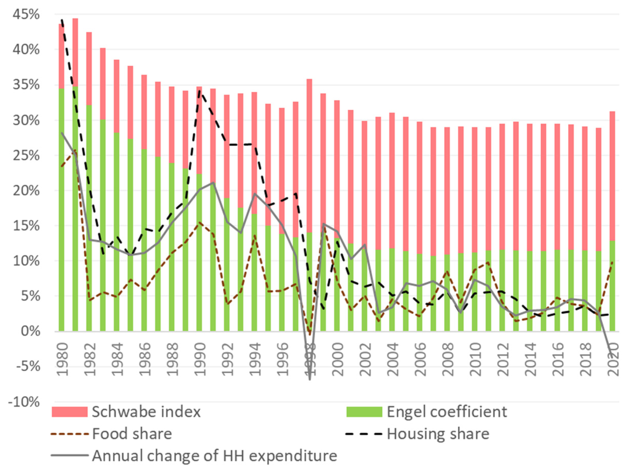
Housing expenditure can be calculated in many ways, and it is closely related to housing affordability, which can be measured in objective and subjective manners. While the subjective approach relies on renters’ assessment of stress levels, the objective method is more numerical and adopts ratio measures. In this regard, three widely accepted ways include the rent-to-income ratio (RIR), Schwabe’s coefficient, and the ratio of housing expenditure to household income [11,18]. RIR concerns a renter’s ability to afford rent and is simply calculated by dividing the monthly rental payment by monthly gross income. It is suggested in many welfare states that no more than 30% of the income be spent on rent [11,19,20,21,22,23,24]. Schwabe’s index, so-called Schwabe’s coefficient, is the proportion of housing costs to a household’s total expenditure, and along with Engel’s coefficient, it is frequently employed to gauge the extent of household poverty [11]. Although Schwabe’s index is disproportionate to household income, it has constantly risen and reached record highs since 2006 [8,10] (Figure 2). Another indicator of housing affordability is the ratio of housing cost to household income, which concerns how much of a household’s income is spent on housing expenses. Compared to RIR, where only rent is considered, the other two methods are more inclusive in that housing-related expenses consist of rent, utilities, home furnishings, equipment, and others. In fact, the share of non-consumption expenditure to urban working households’ total expenditure is on the rise, but the ratio of their consumption expenditure is declining, lagging behind income growth. Nevertheless, the proportion of housing, water, and heating expenses in the consumption expenditure has steadily mounted, reaching a record high of 11.2% in 2020 [8,10] (Figure 2). Therefore, it is more reasonable to adopt the two indicators in this research that assess the proportion of housing expenditure to a household’s living expenses and income in order to assess housing cost burden.

Generally, the standard rule of thumb for housing affordability is that housing expenses should not exceed 30% of the household income. Although the yardstick is widely accepted, 25% does not just serve a more conventional criterion for determining both eligibility and payment levels of public subsidies but provides a more conservative basis for normative housing expenditure [19,23,24]. The focus of this research is on renters, who are often regarded as low-income households since they occupy a lower tier of the housing ladder in terms of housing tenure type, moving from renters to Chonsei to homeowners [25,26,27]. They are more vulnerable to rising housing costs and are directly influenced by market fluctuations [18]. As 25% in this study was selected as a threshold for being cost-burdened, the studied households were the renters spending more than 25% of their income and living expenses on housing costs.

Meanwhile, the state has enforced several codes such as a minimum wage, the standard median income, and the minimum cost of living so as to mitigate the burden of housing costs and enhance the quality of life for households struggling with housing expenses. A minimum wage, distinct from a living wage, is the lowest hourly wage that all employers are required to legally pay employees. The statutory wage decided by the Minimum Wage Council commissioned by the Korea Ministry of Employment and Labor specifies an annual minimum level of wages for workers. In 2020, the minimum wage was 8590 KRW per hour, which equaled 1,795,310 KRW per month for one-person households and 2,991,980 KRW for two-person households [28,29,30] (

Table 1. Standard median income, minimum cost of living, and income eligibility of housing assistance by household size in 2020.

Number of Persons Per Household	Standard Median Income (KRW)	Minimum Cost of Living (KRW)	Income Eligible for Housing Assistance (KRW)
1	1,757,194	1,054,317	790,737
2	2,991,980	1,795,188	1,346,391
3	3,870,577	2,322,347	1,741,760
4	4,749,174	2,849,505	2,137,128
5	5,627,771	3,377,321	2,532,497
6	6,506,368	3,903,821	2,927,866

Note: KRW stands for Korean Won; minimum cost of living is equivalent to 40% of the standard median income, and income eligibility for housing assistance is equivalent to 45% of the standard median income.

). The minimum wage is often compared to the standard median income, which forms the basis for public subsidies. The median income refers to the middle value of national household income annually reviewed and determined by the National Committee of Livelihood Security commissioned by the Korean Ministry of Health and Welfare (KMHW). Based on the standard median income, the minimum cost of living is triennially calculated and announced by KMHW. While serving as the criteria for selecting recipients of public assistance and determining their benefits, the mandated living cost is the amount of money needed to provide basic expenses for living (such as housing, food, utilities, and other necessities). The cost sets forth a reasonable standard of consumption, amounting to 60% of the standard median income (which is related to relative poverty) [29]. As shown in Table 1, the minimum cost in 2020 was 1,054,317 KRW for single-person households. Subsequently, the standard median income determines the amount of housing assistance accounting for 45% of the income [30]. Housing assistance is paid monthly to renters meeting the predetermined income criteria, and the specific amount differs by administrative districts and household size [30] (

Table 2. Monthly payment amount (KRW) of housing assistance by household size and regions in 2020.

Number of Persons	SMA		Non-SMA
	Seoul	GIA	Metropolises	Non-Metropolises
1	266,000	225,000	179,000	158,000
2	302,000	252,000	198,000	174,000
3	359,000	302,000	236,000	209,000
4	415,000	351,000	274,000	239,000
5	429,000	365,000	285,000	249,000
6	504,000	430,000	331,000	291,000

Note: SMA stands for Seoul Metropolitan Area, non-SMA means outside SMA, and GIA stands for GyeongIn Area, which consists of Gyeonggi Province and Incheon Metropolis.

). It is widely recognized that the housing expenses in the SMA are higher than those in non-SMA regions. As a result, the level of housing assistance is adjusted accordingly and in 2020, a monthly payment of 266,000 KRW was provided for single-person households in Seoul.

3. Methods

3.1. Data and Variable Description

The 2020 Korea Housing Survey (KHS) was utilized in this research, and the secondary data underpinned by the Housing Act of 2015 were obtained from the survey biennially conducted from 2006 by the Korea Ministry of Land, Infrastructure and Transportation and annually conducted since 2017 [31,32,33]. The annual survey is the most comprehensive national housing survey, and it aims to provide up-to-date information about households’ quality of residential life and the physical conditions of homes and residential environments. The results of the KHS enable policy makers to make decisions on housing opportunities for people at different levels. The 2020 KHS adopted a structured survey using a face-to-face and door-to-door approach on the spot and included 51,421 households from 23 July to 31 December in 2020 across 17 regions. For the empirical analysis, a sample of 425 cost-burdened households was drawn from the secondary data.

Table 3. Variable description and measurement.

Variables	Description	Unit
Socio-demographic status	Gender	male = 0, female = 1
	Age	years old
	Educational level	<higher education * = 1, ≥higher education = 0
	Household size	two persons and more = 0, single-person = 1
Housing status	Housing structure type	Apartment (APT), single-family home, or others = 0, non-APT multifamily housing = 1
	Housing size	m2
	Number of bedrooms	non-SRO = 0, SRO (single-room occupancy) = 1
	Age of dwelling	≤25 years = 0, >25 years = 1
	Duration of stay in current residence	years
	Receipt of social services	non-recipient = 0, recipient = 1
Economic status	Monthly income	million KRW
	Monthly living expense
	Schwabe’s coefficient	proportion of housing expenses to total living expenses on a monthly basis
	Housing expenditure-to-income ratio	proportion of housing expenses to total household income on a monthly basis
Residential assessment	Housing	4-point Likert scale of satisfaction from 1 (very dissatisfied) to 4 (very satisfied)
	Neighborhood	4-point Likert scale of satisfaction with 9 items (pedestrian safety, school districts, social network, waste management, safety and security, air pollution, outdoor noise, green spaces, and parking lots)
	Urban amenities	4-point Likert scale of satisfaction with accessibility to 5 items (public transit, medical facilities, commercial premise, public institutions, and cultural centers)
	Residential environment	4-point Likert scale of satisfaction

Note: D stands for dummy variable; * <higher education includes primary education and below, lower and upper secondary education.

presents independent and dependent variables and their measurement. The dependent variable is residential assessment, which is measured as the level of each household’s subjective satisfaction with the residential environment on a 4-point Likert scale from 1 (very dissatisfied) to 4 (very satisfied) [34,35]. The residential environment is made up of satisfaction with 15 features including housing, pedestrian safety, school districts, social network, waste management, safety and security, air pollution, outdoor noise, green spaces, parking lots, public transit, medical facilities, commercial premise, public institutions, and cultural centers.

On the other hand, independent variables based on previous studies were largely categorized as socio-demographic status, housing status, and economic status. Socio-demographic variables include each householder’s gender (male or female), age (years old), educational level (primary education and below, lower secondary education, upper secondary education, and higher education and above), employment status (employed or unemployed), and household size (persons per household). Also, housing structure type (single-family home, apartments, and multifamily housing), housing size (m²), number of bedrooms (single-room occupancy, 1-bedroom, and 2-or-more bedroom), age of dwelling (years), duration of stay in current residence (years), decent home (decent or indecent) and social services (recipient or non-recipient) were chosen as housing variables.

Further, economic status includes such variables as asset (million KRW), financial liability (liable or unliable), gross income, and living expense on a monthly basis (million KRW), rent-to-income ratio, Schwabe’s coefficient (percentage), and housing expenditure-to-income ratio. While assets vary from real estate, housing, financial property, and other assets, financial liability is measured as debt or debt-free, and debt includes loans from financial and non-financial institutions as well as rental deposits. Household gross income is a sum of ordinary income earned from regular activities, and non-ordinary income is regarded as the other side of earned or active income and is temporarily unearned or passive income (e.g., money gifts, personal pension annuities, and others). That is, household gross income is each household’s total earnings in the form of wages and salaries, the return on their investments (e.g., dividend, interest, rental property), social benefits (e.g., pensions, public assistance, transfers), and other receipts. Living expenses are a household’s expenditure in a certain period, so the costs of daily living include the amount of money spent on goods and services (e.g., food, health, and education-related services, consumer durables, and housing).

A decent home is determined by whether the current housing conforms to the Statutory Minimum Standard for Housing, which was established in 2000 and revised in 2011. The mandatory standard sets the minimum requirement level for the purpose of health and safety as livable housing in three spheres—dwelling size reflects household size and composition, the number of rooms, and functional fixtures. While dwelling size concerns the minimum floor area for a housing unit needed to accommodate the number of persons in a household, the second regulation considers the minimum number of rooms including the bedroom, dining room, and kitchen [36,37] (

Table 4. Decent home standard in South Korea.

Number of Persons	Household Type	Dwelling Size (m2)	Number of Rooms
1	Single-person household	14	1 BR and 1 K
2	Couple with no child	26	1 BR and 1 DK
3	Parents with one child	36	2 BR and 1 DK
4	Parents with two children	43	3 BR and 1 DK
5	Parents with three children	46
6	Grandparents and parents with two children	55	4 BR and 1 DK

Note: BR stands for bedroom, K for kitchen, and DK for dining room–kitchen.

). The last requirement is laid upon both independent use or separate space of three components—a standing kitchen, a flush toilet, and a shower. A flat unit is regarded as an indecent home when any of the three elements fails to meet the standard.

3.2. Administrative Divisions and Geographic Hierarchy

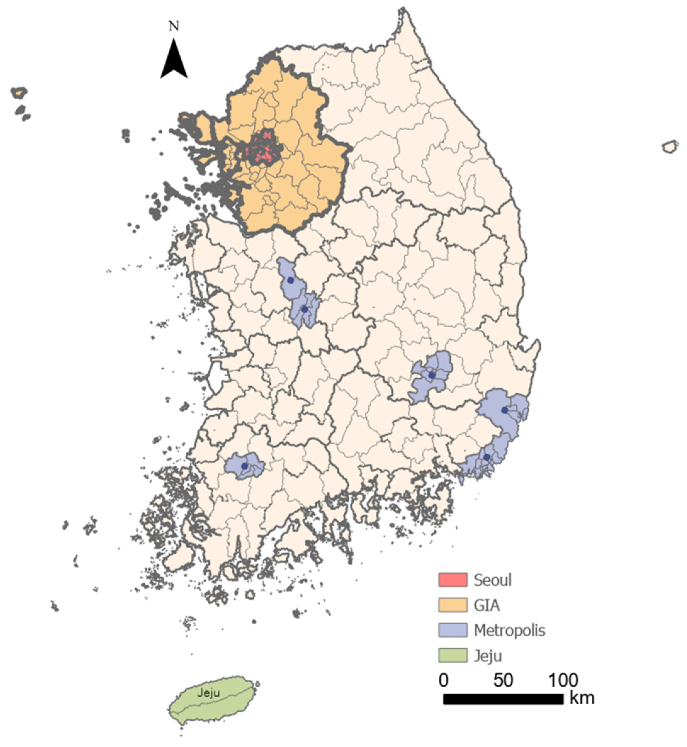
Korea is roughly composed of 229 administrative districts across 17 regions constituting Metropolises and provinces and is generally divided into Seoul Metropolitan Area (SMA) and outside SMA (non-SMA) (Figure 3). While the SMA consists of Seoul, the capital city of the state, and GyeongIn area (GIA) which constitutes Gyeonggi Province and Incheon Metropolis, non-SMA is largely grouped into 6 Metropolises (Busan, Daegu, Gwangju, Daejeon, Ulsan and Sejong) and local self-governing districts of 8 provinces (Gwangwon province located in the eastern side of the SMA and bordered on the east by the East Sea; ChungCheong-Buk and ChungCheong-Nam provinces bounded to the west by the Yellow Sea and adjacent to the SMA; Jeolla-Buk and Jeolla-Nam provinces situated in southwestern Korea, which are bordered by the Yellow Sea; Gyeongsang-Buk and Gyeongsang-Nam provinces located in the southeastern part and bounded on the East Sea; and Jeju province, an island situated in the southwestern part of the Korean peninsula) which are considered to be non-Metropolises.

Only 36.7% of the national territory is habitable, and it is well known as a densely populated nation. In 2020, 51.8 million people lived in a total area of 100,413 km², and the population density was 516.2 people/km² [8,38] (

Table 5. Land area and population density of South Korea.

Items			SMA			Non-SMA
	Total	Subtotal	Seoul	GIA	Subtotal	Metropolises	Non-Metropolises
Area (km2)	100,412.6	11,865.7	605.2	11,260.5	88,546.9	4221.3	84,325.5
	100%	11.8%	0.6%	11.2%	88.2%	4.2%	84.0%
Population (million)	51.8	26.0	9.6	16.4	25.8	10.2	15.6
	100%	50.2%	18.6%	31.6%	49.8%	19.7%	30.1%
Density (people/km2)	516.2	2193.0	15,891.2	1456.7	291.5	2423.1	184.8
Household (million)	20.7	10.1	3.9	6.2	10.6	4.2	6.4
	100%	48.8%	19.1%	29.8%	51.2%	20.1%	31.0%
Persons per household	2.5	2.6	2.4	2.7	2.4	2.5	2.4

Note: BR stands for bedroom, K for kitchen, and DK for dining room–kitchen.

, Figure 4). The SMA accounts for 11.8% of the national territory and accommodates more than half of the total population (50.2%). Conversely, non-SMA in which the rest of the population (49.8%) lives, is the nation’s largest area, constitutes 88.2% of the territory, and is 7.5 times larger than the SMA. While the largest area among the four regions was non-Metropolises (84.0%), followed by GIA (11.2%), Metropolises (4.2%), and Seoul (0.6%), the largest population out of the regions lived in GIA (31.6%), followed by non-Metropolises (30.1%), Metropolises (19.7%), and Seoul (18.6%). In other words, accounted for 0.6% of the territory and 18.6% of the total population (51.8 million people), and GIA held 18.6 times more land (31.6%) but 1.7 times more people (11.2%) than Seoul.

Meanwhile, the area of non-Metropolises (84.0%) was 20 times larger than that of Metropolises (4.2%), but the population in Metropolises (19.7%) was 1.5 times bigger than that in non-Metropolises (30.1%). Thus, the population density varied across regions. The SMA (2193 people/km²) was 7.5 times more populous than non-SMA regions (292 people/km²), and the highest-density region was in Seoul (15,891 people/km²), followed by Metropolises (2423 people/km²), GIA (1457 people/km²), and non-Metropolises (185 people/km²). In other words, Seoul was 11 times more populated than GIA, and Metropolises were 13 times denser than non-Metropolises. On the contrary, more than half of total households lived in non-SMA regions (51.2%) and the largest number of households was in non-Metropolises (31.0%), followed by GIA (29.8%), Metropolises (20.1%), and Seoul (19.1%). Given the population and number of households, the average household size was larger in non-SMA regions (2.4 persons) than in the SMA (2.6 persons), and the largest size was in GIA (2.7 persons), followed by Metropolises (2.5 persons), Seoul, and non-Metropolises (2.4 persons).

3.3. Data Analysis

Data used in the study were obtained from publicly available sources accessible on the MicroData Integration Service (MDIS) homepage [33], and IBM SPSS Statistics version 29.0 was utilized for statistical analyses. The analyses included both descriptive analysis using the mean and standard deviation (SD) and inferential analysis containing a chi-square (χ²) test, one-way analysis of variance (ANOVA), factor analysis, and multiple regression analysis. For multiple regression analysis, some explanatory variables were treated as dummy ones valued 0 or 1, and the binary variables are listed in Table 3.

The statistical model is expressed as an equation below:

Ƴ_ra = β₀ + β₁Χ_sds + β₂Χ_hsg+ β₃Χ_ecs + β₄Χ_req + ε

The dependent variable on the left side refers to the subjective satisfaction with the residential environment, which is substituted for the residential assessment. On the right side, β₀ refers to the constant term, β₁ to the socio-demographic status, β₂ to housing status, β₃ to economic status, β₄ to residential environment qualities, and ε to an error term. The significance level was set at 0.05.

4. Results

4.1. General Characteristics of Housing Cost-Burdened Renters

4.1.1. Socio-Demographic Status

More than half of housing cost-burdened households (225 households) lived in non-SMA regions (51.9%) and the rest (200 households) resided in the SMA (47.1%). Geographically, many of them were concentrated in Seoul (135 households, 29.4%), followed by non-Metropolises of non-SMA regions (116 households, 27.3%), Metropolises of non-SMA regions (109 households, 25.6%), and GIA (75 households, 17.6%). The gender of the studied householders was predominantly male and the number of male householders was twice as high as their counterparts. More female householders were found in non-Metropolises than in the other regions where the share of male householders ranged from 3/5 to 3/4 (65.1~77.3%) (

Table 6. Socio-demographic, housing, and economic statuses of housing cost-burdened households by administrative districts.

Variables		Seoul (A)	GyeongIn Area (B)	Metropolises (C)	Non-Metropolises (D)	Χ2/F (ρ) (A–D)
		f (%) or Mean ± SD
Gender	Male	86 (68.8)	58 (77.3)	71 (65.1)	65 (56.0)	9.880 (0.020)
	Female	39 (31.2)	17 (22.7)	38 (34.9)	51 (44.0)
Age (years old)		52.9 ± 19.6	54.4 ± 15.2	54.8 ± 17.1	56.4 ± 17.7	0.906 (0.688)
Educational level	≤Primary education	23 (18.4)	8 (10.7)	33 (30.3)	38 (32.8)	33.958 (0.000)
	Lower secondary	40 (32.0)	20 (26.7)	26 (23.9)	11 (9.5)
	Upper secondary	41 (32.8)	34 (45.3)	39 (35.8)	54 (46.6)
	≥Higher education	21 (16.8)	13 (17.3)	11 (10.1)	13 (11.2)
Employment status	Employed	61 (48.8)	31 (41.3)	37 (33.9)	55 (47.4)	6.344 (0.096)
	Unemployed	64 (51.2)	44 (58.7)	72 (66.1)	61 (52.6)
Household size		1.3 ± 0.8	1.4 ± 1.0	1.3 ± 0.9	1.6 ± 1.1	1.535 (0.165)
Housing structure type	Apartment (APT)	3 (2.4)	2 (2.7)	1 (0.9)	5 (4.3)	76.484 (0.000)
	Single-family home	8 (6.4)	3 (4.0)	13 (11.9)	32 (27.6)
	Non-APT multifamily housing	108 (86.4)	68 (90.7)	83 (76.1)	51 (44.0)
	Other	6 (4.8)	2 (2.7)	12 (11.0)	28 (24.1)
Housing size (m2)		12.6 ± 11.4	16.0 ± 19.6	20.5 ± 20.4	29.8 ± 24.0	5.200 (0.000)
Number of bedroom	Single-room occupancy (SRO)	107 (85.6)	65 (86.7)	74 (67.9)	60 (51.7)	45.124 (0.000)
	One	11 (8.8)	4 (5.3)	16 (14.7)	25 (21.6)
	Two and more	7 (5.6)	6 (8.0)	19 (17.4)	31 (26.7)
Age of dwelling (years)	≤25	45 (47.9)	24 (77.4)	23 (26.1)	32 (41.0)	26.271 (0.000)
	>25	49 (52.1)	7 (22.6)	65 (73.9)	46 (59.0)
Duration of stay in current residence (years)		3.2 ± 5.2	3.3 ± 4.7	4.1 ± 5.7	6.9 ± 8.1	1.943 (0.004)
Social service	Recipient	31 (24.8)	24 (32.0)	50 (45.9)	39 (33.6)	11.719 (0.008)
	Non-recipient	94 (75.2)	51 (68.0)	59 (54.4)	77 (66.4)
Asset (million KRW)		8.8 ± 22.3	10.9 ± 38.5	11.2 ± 49.2	15.0 ± 32.2	1.575 (0.004)
Monthly income (million KRW)		1.1 ± 0.6	1.1 ± 0.8	0.8 ± 0.4	1.0 ± 0.6	1.538 (0.006)
Monthly living expenses (million KRW)		0.8 ± 0.4	0.9 ± 0.6	0.7 ± 0.3	0.8 ± 0.5	1.641 (0.009)
Monthly rent (million KRW)		0.34 ± 0.14	0.33 ± 0.20	0.27 ± 0.14	0.32 ± 0.23	2.373 (0.000)
Rent-to-income ratio (RIR)		37.2 ± 16.7	36.2 ± 13.2	36.1 ± 21.1	34.2 ± 20.1	1.640 (0.000)
Schwabe’s coefficient		59.2 ± 66.8	45.7 ± 15.1	41.7 ± 13.1	48.1 ± 20.4	1.415 (0.006)
Housing expenditure-to-income ratio		42.1 ± 18.4	39.5 ± 12.2	43.8 ± 28.4	44.9 ± 28.1	1.281 (0.036)

Note: KRW stands for Korean Won and SD for standard deviation; the average USD/KRW exchange rate for 2020 was 1 USD equal to 1190 KRW.

). In particular, the region with the highest proportion of male householders was GIA, where there were 3.4 times male heads more than female ones. Although there was no significant difference in the age of the householders across the regions, the overall average age was between the ages of 53 and 56—the oldest was in non-Metropolises (56.4 years old) and the youngest in Seoul (52.9 years old). Also, the largest segment in the age structure was the late middle-aged group (50–64) and the elderly group (65+), of which both accounted for three-fifths (67.8%), and the two groups were 2.1 times larger than the others consisting of the young group (19–34) and early middle-aged group (35–49). With regard to the geographical distribution by age groups, the young group was the highest in Seoul (26.4%), the late middle-aged group in GIA (44.0%), and the elderly group in non-Metropolises (36.2%) and Seoul (33.6%). In contrast, the middle-aged group was the most economically active and was the lowest portion (8.8–19.0%) in all regions where the gap between the largest and smallest regions amounted to 2.2 times.

The educational levels of a householder were classified into four stages ranging from primary education and below (elementary school graduate and no formal education), lower secondary education (middle school graduate), upper secondary education (high school graduate), to higher education and above (college graduate and higher degree). Overall, high school graduates were the most dominant group (39.5%), followed by middle school graduates (22.8%) and elementary school graduates or below (24.0%), then college graduates and higher (13.6%). Geographically, the proportion of elementary school graduates was higher in the SMA (18.4% in Seoul and 10.7% GIA) than in non-SMA regions (32.8% in non-Metropolises and 30.3% in Metropolises). On the other hand, the share of middle school graduates was higher in non-SMA regions (23.9% in Metropolises and 9.5% in non-Metropolises) than in the SMA (32.0% in Seoul and 26.7% GIA). The percentage of high school graduates was the highest in the four regions, and in particular, both non-Metropolises (46.6%) and GIA (45.3%) were higher than the other two regions. However, the lowest share was observed in the segment of college graduates and holders of higher degrees, and the ratio was higher in the SMA (17.3% in GIA and 16.8% in Seoul) than in non-SMA regions (11.2% in non-Metropolises and 10.1% in Metropolises).

More than half of the householders in the four regions were unemployed (56.7%), and the unemployment rate was a little higher in Metropolises (66.1%) and GIA (58.7%) than in Seoul (48.8%) and non-Metropolises (47.4%). Three-fourths of the employed householders were salaried workers (76.6%), and the proportion of the workers was higher in the SMA (96.7% in Seoul and 87.1% in GIA), while self-employed heads were found to be higher in non-SMA regions (47.3% in non-Metropolises and 29.7% in Metropolises). The average household size was 1.5 persons, and non-Metropolises recorded the largest size of 1.6 persons per household. With respect to household types, single-person households were the most common household form (overall 80.0%), and the households were prevalent in all regions (85.6% in Seoul, 83.5% in Metropolises, and 82.7% GIA) but non-Metropolises (31.0%) in which multi-person households were more common. Since household size is closely associated with marital status, a vast majority of the householders were not married (92.9%), and the portion of married householders was relatively high in non-Metropolises (12.1%). Not surprisingly, an overwhelming majority of the households had no children, and childless households were predominant in the regions (94.4% in Seoul, 90.7% in GIA, and 89.9% in Metropolises) where single-person households were widespread. On the contrary, the equal number of households with children was found in non-Metropolises where the percentage of multi-person households was somewhat high.

4.1.2. Housing Status

The cost-burdened renters primarily resided in multifamily housing (72.9%), followed by single-family homes (13.2%), others (11.3%), and apartments (APTs) (2.6%) (Table 6). Although APTs, a form of multifamily housing, are widely recognized as housing for middle-class people and have been considered to be the modern housing structure norm, the category of non-APT multifamily housing is extensively perceived to be more affordable than APTs. It is shown that most people in the SMA (90.7% in GIA and 86.4% in Seoul) dwelled in non-APT multifamily housing, whereas the proportion of living in single-family homes (27.6%) and other types of housing (24.1%) was considerably high in non-Metropolises, where the percentage of non-APT multifamily housing (44.0%) was the lowest among the regions.

Current housing size is the floor area of a dwelling measured in square meters, and the largest housing size was found to be in non-Metropolises (29.8 m²) where RIR was the lowest among the regions, followed by Metropolises (20.5 m²), GIA (16.0 m²), and Seoul (12.6 m²) in which housing expenses were higher than the others. The size difference between the largest (non-Metropolises) and the smallest (Seoul) was 2.4 times. A majority of the renters lived in a single-room occupancy (SRO) unit (72.0%), which was predominant in the SMA (86.7% in GIA and 85.6% in Seoul), but more renters in non-SMA regions (48.3% in non-Metropolises and 32.1% in Metropolises) lived in a dwelling with individual separate bedrooms. About three-fifths (59.0%) of the households resided in old housing that was built more than 25 years ago. The proportion of households living in old housing was highest in Metropolises (73.9%), followed by non-Metropolises (59.0%), Seoul (52.1%), and GIA (22.6%). Unlike the other three regions, GIA has been steadily supplied with new housing driven by New Town Development projects for decades, so more than three-quarters of the households in GIA lived in relatively new housing. By contrast, approximately three-quarters in Metropolises resided in old houses.

The average length of stay In the current residence was longer in non-SMA regions (6.9 years in non-Metropolises and 4.1 years in Metropolises) than in the SMA (3.3 years in GIA and 3.2 years in Seoul). The duration difference between non-Metropolises and Seoul was 2.1 times. While all of the renters lived in dwellings that met the statutory minimum standard for housing, only a third of total households relied on social services, and the public dependence was higher in non-SMA (45.9% in Metropolises and 33.6% in non-Metropolises) than in the SMA (32.0% in GIA and 24.8% in Seoul).

4.1.3. Economic Status

Three-fifths of the cost-burdened renter households possessed any amount of assets (62.6%), and the largest percentage of asset-holders was found in non-Metropolises (80.2%), followed by Metropolises (59.6%), GIA (57.3%) and Seoul (52.0%) (Table 6).

The average value of total assets among asset-holders varied with regions, and the largest value was in non-Metropolises (15.04 million KRW), followed by Metropolises (11.21 million KRW), GIA (10.91 million KRW), and Seoul (8.86 million KRW). The value discrepancy between non-Metropolises and Seoul was 1.7 times, and the average asset value in Seoul was equal to about three-fifths (58.9%) of that in non-Metropolises. A vast majority of the renters (89.9%) were debt-free, indicating that only one out of ten renters had financial liability.

Many of the householders were unemployed older adults aged 50 and over, so their average monthly income fell between 0.80 and 1.08 million KRW, which was well below the minimum wage (1.79 million KRW). Although there was no significant distinction in monthly income across the regions, the average income in the SMA (1.08 million KRW in Seoul and 1.06 million KRW in GIA) was slightly higher than in non-SMA regions (0.99 million KRW in non-Metropolises and 0.80 million KRW in Metropolises). Given the fact that single-person households were dominant in four regions, the average household income was far below the standard median income for single-person households (1.76 million KRW). While the average monthly living expenses were nearly the same across the regions (0.88 million KRW in GIA, 0.85 million KRW in non-Metropolises, 0.80 million KRW in Seoul, and 0.76 million KRW in Metropolises), it fell short of the minimum cost of living, posing a serious threat to survival. Although no significant difference in the amount of rent deposits was found across the regions, Seoul had the largest amount (10.98 million KRW), which was 1.5 times greater than the smallest amount (7.12 million KRW in Metropolises). Monthly rent varied with regions (0.27–0.35 million KRW), and the rent was slightly higher in the SMA (0.35 million KRW in Seoul and 0.33 million KRW in GIA) than in non-SMA regions (0.32 million KRW in non-Metropolises and 0.27 million KRW in Metropolises). The rent interval between the highest and lowest regions was 1.3 times.

The housing cost burden of the renters was measured in three indices—rent-to-income ratio (RIR), Schwabe’s index, and housing expenditure-to-income ratio. All three indices exceeded 30% of the housing poverty level, and the RIR was roughly the same in all regions (37.2% in Seoul, 36.2% in GIA, and 36.1% in Metropolises) but non-Metropolises, in which it was the lowest (34.2%). As for Schwabe’s index, Seoul showed the highest (59.2%), and three-fifths of the expenditure was spent on housing expenses, presenting a serious and significant danger. The rest exceeded more than two-fifths (48.1% in non-Metropolises, 45.7% in GIA, and 41.7% in Metropolises), and the gap between the highest and lowest regions was 17.6%. Thus, the findings indicate that all the households experienced shelter poverty. The housing expenditure-to-income ratio showed geographic similarity, and the ratio was higher in non-SMA regions (44.9% non-Metropolises and 43.8% in Metropolises) than in the SMA (42.1% in Seoul and 39.5% in GIA), demonstrating that this was partially attributed to income disparity across the regions. Since the studied households were selected based on two indices exceeding 25%, both Schwabe’s index and housing expenditure-to-income ratio were extremely high in all regions, especially in Seoul, where housing and its related costs are pretty high. The results reveal that all the renters clearly suffered from shelter poverty, and public intervention is imperative to immediately alleviate the burden.

4.2. Residential Environment Qualities and Assessment of Housing Cost-Burdened Renters

The residential environment has a variety of facets in houses and their physical surroundings, and the built environment embraces collective attributes affecting the quality of human life. Residential environment qualities include housing and overall residential environment, which contains the fourteen domains of pedestrian safety, school districts, social network, waste management, safety and security, air pollution, outdoor noise, green spaces, parking lots, public transit, medical facilities, commercial premise, public institutions, and cultural centers. All of the sixteen features were subjectively evaluated by cost-burdened renters, and the assessment was compared across the four distinctive regions. The results showed that even though satisfaction with housing and the overall residential environment was not statistically significant among the regions, all the households were more satisfied with the residential environment than housing but both satisfaction levels were slightly higher in Seoul than in the other regions (

Table 7. Residents’ satisfaction with housing and residential environment.

Variables	Satisfaction Level				F(ρ) (A–D)
	Seoul (A)	GIA (B)	Metropolises (C)	Non-Metropolises (D)
Housing	2.74	2.56	2.62	2.56	2.049 (0.106)
Residential environment	2.91	2.85	2.81	2.86	0.635 (0.593)

). Out of the 14 items, statistically significant differences among the regions were found in 8 variables—social network, green spaces, parking lots, public transit, medical facilities, commercial premises, public institutions, and cultural centers. Moreover, the statistical findings revealed the highest satisfaction with accessibility to public transit and the lowest satisfaction with parking lots in all the regions except non-Metropolises, in which the households showed the highest satisfaction with green spaces and the lowest satisfaction with cultural centers.

With regard to satisfaction with accessibility to 14 elements, an Exploratory Factor Analysis (EFA) is presented to demonstrate the accuracy of the analysis, resulting in two factors (

Table 8. Assessment of residential environment quality.

Variables		SMA		Non-SMA		F(ρ) (A–D)	Overall		Cronbach’s α
		Seoul (A)	GIA (B)	Metropolises (C)	Non-Metropolises (D)		1	2
Neighborhood	Pedestrian safety	2.93	2.99	2.95	3.05	1.071 (0.361)	0.670		0.862
	School districts	2.93	2.77	2.87	2.82	2.547 (0.056)	0.591
	Social network	2.93	2.75	2.69	2.88	3.281 (0.021)	0.654
	Waste management	2.90	2.81	2.94	2.92	1.594 (0.190)	0.716
	Safety and security	2.89	2.84	2.90	2.96	1.356 (0.256)	0.764
	Air pollution	2.81	2.81	2.90	2.97	2.087 (0.101)	0.807
	Outdoor noise	2.77	2.60	2.76	2.74	0.502 (0.681)	0.731
	Green spaces	2.77	2.89	2.91	3.17	6.028 (0.001)	0.459
	Parking lots	2.52	2.51	2.69	2.80	4.573 (0.004)	0.616
Urban amenities	Public transit	3.28	3.23	3.18	3.04	6.092 (0.000)		0.746	0.893
	Medical facilities	3.17	3.04	3.03	2.85	8.135 (0.000)		0.883
	Commercial premise	3.17	3.17	3.05	2.90	7.678 (0.000)		0.849
	Public institutions	3.12	2.99	3.09	2.93	4.574 (0.004)		0.842
	Cultural centers	2.83	2.68	2.83	2.54	2.786 (0.040)		0.798
	KMO						0.913
Bartlett	Chi-square						2901.574
	df (p)						91 (0.000)

). The Kaiser–Meyer–Olkin (KMO) measure of sampling adequacy was 0.913 (KMO > 0.7), indicating that the correlation between the selected influencing factors was strong [39,40]. Bartlett’s test of sphericity had a significant value = 0.000 (ρ < 0.05), showing that the correlation coefficient matrix was not a unit matrix. Along with the output of chi-square (2901.574, df = 91), the results specify that the data meet the prerequisites for factor analysis. Factor loading values that were less than 0.5 were eliminated, and in the extraction of the EFA, initial eigenvalues greater than 1 were eliminated [41,42]. Further, the reliability of the questionnaire in terms of the two factors was assessed on the basis of Cronbach’s alpha coefficient. Cronbach’s alpha coefficients of 0.7 or higher are recognized as acceptable values. The values of the coefficient were acceptable for the two factors, ranked from 0.862 to 0.893. Therefore, the two factors were determined with factor 1 labeled as “neighborhood” and factor 2 as “urban amenities”. While three variables, including social network, green spaces, and parking lots, were grouped in factor 1 of neighborhood, five items such as public transit, medical facilities, commercial premise, public institutions, and cultural centers were assigned to factor 2 of urban amenities. With a total of eight variables from the two factors, there was a significant difference in the satisfaction levels between Seoul and non-Metropolises. Indeed, the highest satisfaction with urban amenities in Seoul clearly differed from the lowest satisfaction in non-Metropolises. For satisfaction with the neighborhood, the households in Seoul were more satisfied with the social network but less satisfied with green spaces and parking lots than those residing in non-Metropolises.

4.3. Predictors for Residential Assessment

To investigate the predictors affecting the residential assessment of housing cost-burdened households, a multiple regression analysis with an enter method was employed, and its results are summarized in

Table 9. Regression analysis for predicting residential assessment of housing cost-burdened households by administrative districts.

Variables		SMA						Non-SMA
		Seoul			GyeongIn Area			Metropolises			Non-Metropolises
		β	SE	ρ	β	SE	ρ	β	SE	ρ	β	SE	ρ
Constant			0.475	0.798		0.606	0.765		0.486	0.013		0.495	0.033
Female householder (D)		0.037	0.082	0.521	−0.050	0.133	0.650	−0.084	0.075	0.307	−0.064	0.100	0.415
Age of householder		−0.026	0.002	0.727	0.040	0.004	0.699	0.027	0.003	0.792	−0.039	0.004	0.729
Under higher education (D)		0.062	0.120	0.364	−0.131	0.134	0.196	−0.058	0.124	0.497	−0.088	0.165	0.281
1-person household (D)		−0.062	0.145	0.427	−0.326	0.209	0.040	0.058	0.115	0.554	−0.079	0.136	0.425
Non-APT multifamily housing (D)		−0.057	0.127	0.389	0.120	0.254	0.412	0.370	0.098	0.000	−0.041	0.112	0.634
Housing size		0.110	0.006	0.267	0.107	0.005	0.585	0.106	0.002	0.346	0.009	0.002	0.925
Single-room occupancy (D)		0.077	0.155	0.352	0.112	0.239	0.486	0.064	0.122	0.622	−0.020	0.127	0.839
Old dwelling (D)		0.081	0.091	0.231	−0.014	0.216	0.909	0.195	0.081	0.033	0.041	0.109	0.621
Duration of stay		−0.021	0.008	0.752	0.048	0.014	0.709	0.004	0.007	0.967	−0.006	0.007	0.949
Social service recipient (D)		−0.048	0.097	0.450	0.124	0.108	0.215	−0.106	0.082	0.259	−0.130	0.123	0.153
Asset		0.121	0.000	0.064	−0.068	0.000	0.484	0.134	0.000	0.088	−0.065	0.000	0.430
Income		−0.141	0.001	0.163	−0.151	0.001	0.432	0.121	0.001	0.228	−0.151	0.001	0.134
Schwabe’s coefficient		0.075	0.001	0.257	−0.085	0.005	0.523	−0.222	0.003	0.029	−0.122	0.003	0.127
Housing expenditure-to-income ratio		−0.064	0.003	0.460	0.171	0.006	0.208	0.333	0.002	0.005	0.030	0.002	0.732
Satisfaction with	Housing	0.471	0.091	0.000	0.011	0.096	0.913	0.326	0.076	0.001	0.191	0.080	0.031
	Neighborhood	0.255	0.127	0.015	0.452	0.156	0.000	−0.009	0.125	0.915	0.240	0.133	0.010
	Urban amenities	0.183	0.109	0.028	0.303	0.114	0.009	0.184	0.070	0.041	0.430	0.078	0.000
R2		0.686			0.572			0.547			0.552
R2adj.		0.636			0.445			0.462			0.474
F(p)		13.734 (0.000)			4.485(0.000)			6.453(0.000)			7.102(0.000)

Adjusted variables including female householder (D), age, and educational level (D) of householder, single-person household (D), monthly income, Schwabe’s coefficient, housing expenditure-to-income ratio, total asset, multifamily housing (D), housing size, more than 25-year-old dwelling (D), age of residence, social service recipients (D), and satisfaction with housing, neighborhood, and urban amenities.

. While the dependent variable was the overall satisfaction with the residential environment measured on a four-point scale (from very dissatisfied (1) to very satisfied (4)), the independent variables consisted of socio-demographic attributes (gender, age, and educational level of a householder), housing features (housing structure type, housing size, number of bedrooms, age of dwelling, duration of stay in current residence, and dependence on social services), economic characteristics (asset, income, Schwabe’s coefficient, and housing expenditure-to-income ratio), and residential environment qualities (housing satisfaction, neighborhood satisfaction, and satisfaction with urban amenities). Some of the independent variables were treated as dummy variables representing one category of the explanatory variable. For instance, they were coded with 1 to depict a female householder, a householder with a higher educational level, a single-person household, non-APT multifamily housing, a single-room occupancy unit, an old dwelling, and a recipient of social services.

The results of multiple linear regression analysis showed that four regression models across the regions were statistically significant at the 1% level, and the explanatory power of the linear model ranged from 44.5% to 63.6%. Even though predictors for the residential assessment of the renter households varied with regions, the common determinant of residential assessment across the regions was satisfaction with urban amenities. The overall satisfaction was positively associated with satisfaction with neighborhoods in Seoul, GIA, and Metropolises, and housing satisfaction in Seoul, Metropolises, and non-Metropolises. Also, satisfaction with the residential environment was negatively influenced by single-person households in GIA and by Schwabe’s coefficient in Metropolises, of which the dependent variable was also positively affected by housing expenditure-to-income ratio, non-APT multifamily housing, and old dwellings. In other words, residential satisfaction in Seoul and non-Metropolises was higher among the households who were satisfied with housing, neighborhood, and urban amenities. In GIA, satisfaction increased among households who were satisfied with neighborhood and urban amenities, but the level decreased among single-person households. Although residential satisfaction in Metropolises was higher among households who had high housing expenditure-to-income ratios, lived in non-APT multifamily housing and old dwellings, and were satisfied with housing and urban amenities, the level was lower among those with high Schwabe’s coefficients.

5. Discussion

This empirical research focused on renter households spending more than 25% of both their income and living expenses on housing costs, and the cross-sectional study compared their socio-demographic, economic, and housing statuses in four distinctive regions—Seoul and GyeongIn Area (GIA) of the Seoul Metropolitan Area (SMA) and Metropolises and non-Metropolises outside the SMA (non-SMA). Also, statistical analysis was employed to determine the factors influencing their subjective assessment of the residential environment, and the main findings are summarized as follows. Firstly, most of the renter households were unemployed single men with upper secondary education or lower, aged in their mid-50s, and the portion of two or more households and female householders was relatively high in non-Metropolises of non-SMA regions. While age, educational attainment, and employment status of householders were interrelated, the share of unemployed householders with primary education or lower was high in both Seoul and non-Metropolises where the percentage of elderly households was somewhat high. Also, the proportion of employed householders with upper secondary education was high in both GIA, where the share of late middle-aged householders was relatively high, and in Metropolises.

Regardless of the region, all the renters resided in decent homes that fulfilled the statutory minimum standard for housing, most lived in old non-APT multifamily housing, and many did not rely on social services. Compared to other regions, most householders in Seoul resided in the smallest houses, and the share of living in relatively new dwellings was high in GIA. While more social service recipients were found in Metropolises, householders in non-Metropolises lived in more spacious housing with separate bedrooms for a longer period than any other region. Thirdly, most renter households possessed some amount of assets and were debt-free, and more than half of them were unemployed, late middle-aged householders with low incomes. While household income was significantly below the minimum wage and well below the standard median income, living expenses fell short of the minimum cost of living, and more than half of the expenses were allocated to housing-related costs, putting the households’ livelihood at risk. Due to a proportionately linear relationship among income, deposit, and rent, the highest values of the three variables were observed in Seoul, followed by GIA, non-Metropolises, and Metropolises. For all the renters, the average housing cost-related indices, including rent-to-income ratio (RIR), Schwabe’s coefficient, and housing expenditure-to-income ratio, exceeded 30%, indicating an extremely high level of housing cost burden and housing poverty. Evidently, the households face a worsening of poverty and even greater threats to survival.

With respect to the spatial discrepancy of the housing cost burden, Seoul, with the highest income, deposit, and rent, demonstrated the highest values in both the RIR and Schwabe’s coefficient. Although GIA shared a comparable level of income with Seoul, it had the highest living expenses and the lowest housing expenditure-to-income ratio. Metropolises had the lowest values in income, deposit, rent, living expenses, and Schwabe’s coefficient, whereas non-Metropolises recorded the lowest RIR while the housing expenditure-to-income ratio peaked. Therefore, housing cost burden indices varied with regions. While regional differences in rent, living expenses, and income were closely associated with unequal housing cost burdens, the findings imply that lower rent or income increases could substantially alleviate the burden. For instance, non-Metropolises with relatively low rent had a lower RIR than any other region. On the contrary, GIA, which had similar income levels to Seoul but the highest cost of living among the regions, showed a much lower RIR, Schwabe’s coefficient, and housing expenditure-to-income ratio than Seoul. In particular, its housing expenditure-to-income ratio was the lowest among regions. While Metropolises, with the lowest income and living expenses, had the lowest Schwabe’s coefficient, their RIR was similar to that of GIA, and their housing expenditure-to-income ratio was higher than that of Seoul. Fourthly, there was no statistical significance in regional differences in satisfaction with housing and the residential environment. All the households across regions tended to be more satisfied with the residential environment than with housing, and the residential satisfaction appeared to be higher in Seoul than in any other region. Moreover, the satisfaction with public transit among the 14 residential environment qualities was highest in Seoul, GIA, and Metropolises, while the highest satisfaction with green spaces and the lowest with cultural centers was observed in non-Metropolises. Factor analysis revealed that the 14 elements were classified into two factors—neighborhood and urban amenities. Regional distinctions were statistically significant in three components of the first, including social networks, green spaces, and parking lots, and also in the five constituents of the second consisting of public transit, medical facilities, commercial premise, public institutions, and cultural centers. Generally, most of the households among the regions were more satisfied with urban amenities than neighborhoods.

The results of the regression analysis elicited that satisfaction with urban amenities was the most important determinant of residential assessment across the four regions. In addition, satisfaction with the neighborhood was determined to be a common predictor in Seoul, GIA, and Metropolises, and housing satisfaction was also observed to have statistical significance in Seoul, Metropolises, and non-Metropolises. For Metropolises, explanatory variables such as non-APT multifamily housing, housing expenditure-to-income ratio, Schwabe’s coefficient, and old dwellings were found to be statistically significant. Therefore, all the housing cost-burdened renter households who were satisfied with urban amenities were likely to have increased satisfaction with the residential environment. In Seoul, GIA, and Metropolises, the households who were satisfied with the neighborhood showed a high level of overall residential satisfaction. Also, the renters who were satisfied with housing in Seoul, Metropolises, and non-Metropolises perceived their overall satisfaction with the residential environment as satisfactory. In Metropolises, the households residing in old non-APT multifamily housing, with a high housing expenditure-to-income ratio and a low Schwabe’s coefficient, were satisfied with their residential environment.

6. Conclusions

With the perception that housing is not merely a shelter fulfilling basic needs for daily life, the Housing Act of 2022 in Korea viewed housing as part of human rights, which is embedded into the policy paradigm emphasizing the quality sphere of housing [36]. In fact, it is significant to enable all to obtain access to adequate and affordable housing. Since the Statutory Minimum Standard for Housing has been in effect since 2000, decent and adequate housing, as a physical facet of housing, has been largely supplied and widely available. While all the renters in this study lived in decent homes, the importance of housing affordability, as an economic domain of housing, still became explicit in determining their quality of life. In the conventional housing ladder, renters occupying the lower rung are frequently seen as a socio-economically vulnerable group relying on both housing assistance and social services. As the rent sector continues to expand and housing-related expenses are elevated, the financial strain disproportionately affects renter households. In this context, this research focused on renters burdened by housing costs and examined their spatial variations. Most of the renters were unemployed individuals living alone with lower levels of educational attainment, resided in old non-APT multifamily flats meeting the statutory minimum standard for housing, did not rely on social services, and owned assets without financial obligations. These socio-demographically and economically vulnerable statuses indicate many implications. With income below both the minimum wage and the standard median income and living expenses below the minimum cost of living, overspending on housing expenses has trapped them in poverty, and it undoubtedly presents a serious threat to survival for those who do not receive social services.

In spite of the commonality of housing cost overburden, the spatial discrepancies in socio-economic statuses and residential quality stem from local housing markets reflecting the interplay of demand and supply issues at both macro and micro levels (e.g., labor market, wages, financial consideration, and regulations). Indeed, an extended period of low interest rates and economic downturn favored a shift in the rental sector from Chonsei to renting, and the rapid transition led to an increase in housing expenses, which in turn exacerbated the financial burden for renter households. Therefore, it is of importance to tackle the housing cost burden through multiple interventions tailored to both local needs and the overburdened households. Specifically, housing assistance or public rental housing can substantially alleviate the burden, and cash transfer can stimulate not just income growth but spending power. Simultaneously, it is crucial to constantly monitor any changes in the socioeconomic and housing statuses of the renters (e.g., income and age of renters, household size, housing structure type, housing size, and housing age), with a particular emphasis on tracking the housing expenditures of renters in Seoul, where housing expenses are notably high, and non-SMA regions, where incomes are lower. Further, working-age renters should be provided with economic opportunities including employment, paid training, and access to long-term, low-interest housing loans in order to get out of housing poverty and to accumulate housing capital which can serve as seed money for upward mobility on the housing ladder. More importantly, the public housing programs on both supply and demand sides should be revised and elaborated with detailed eligibility criteria, aiming for greater inclusiveness and resilience.

References

- Doling, J. Housing policies and the little tigers. Hous. Stud. 1999, 14, 229–250. [Google Scholar] [CrossRef]
- Lee, H. Housing and socioeconomic transformations in South Korea. In Housing East Asia: Socioeconomic and Demographic Challenges; Doling, J., Ronald, R., Eds.; Palgrave Macmillan: London, UK, 2014; pp. 180–203. [Google Scholar] [CrossRef]
- Lim, S.H. A Half Century of Korean Housing Policy; Gimundang: Seoul, Republic of Korea, 2005. [Google Scholar]
- Ronald, R. The Ideology of Home Ownership: Homeowner Societies and the Role; Palgrave Macmillan: London, UK, 2008. [Google Scholar]
- Lee, H. Changing Korean housing system and its structural forces. J. Asian Archit. Build. Eng. 2017, 16, 519–526. [Google Scholar] [CrossRef]
- Lee, H. Changing household and housing statuses in shrinking cities of non-Seoul Metropolitan Area. J. Korean Hous. Assoc. 2021, 32, 59–70. [Google Scholar] [CrossRef]
- Lee, H.; Park, J.H. Constructing a conceptual framework of smart ageing bridging sustainability and demographic transformation. Land Hous. Rev. 2023, 14, 1–16. [Google Scholar] [CrossRef]
- Statistics Korea. KOSIS Statistical Database. Available online: https://kosis.kr/eng/ (accessed on 4 December 2023).
- Kwon, Y.H.; Choi, Y. A study on the residential upward and downward mobility in one-person households by age characteristics. Korea Spat. Plan. Rev. 2018, 99, 97–112. [Google Scholar] [CrossRef]
- Bank of Korea. Economic Statistics System. Available online: https://ecos.bok.or.kr/#/ (accessed on 4 December 2023).
- Lee, H.; Kim, D.; Jeong, C. Socioeconomic distinctions and determinants of housing expenditure for home-owning and renting households. J. Korean Hous. Assoc. 2018, 29, 59–70. [Google Scholar] [CrossRef]
- Groves, R.; Murie, A.; Watson, C. Housing and the New Welfare State; Ashgate Publishing Limited: Hampshire, UK, 2007. [Google Scholar]
- Hirayama, Y.; Ronald, R. Housing and Social Transition in Japan; Routledge: London, UK, 2007. [Google Scholar]
- Holliday, I.; Wilding, P. Welfare Capitalism in East Asia; Palgrave Macmillan: New York, NY, USA, 2003. [Google Scholar]
- Lee, H. Institutional shifts of four East Asian developmental housing systems. J. Asian Archit. Build. Eng. 2018, 17, 103–110. [Google Scholar] [CrossRef]
- Forrest, R.; Lee, J. Housing and Social Change: East-West Perspectives; Routledge: London, UK, 2003. [Google Scholar] [CrossRef]
- Doling, J.; Ronald, R. Housing East Asia: Socioeconomic and Demographic Challenges; Palgrave Macmillan: London, UK, 2014. [Google Scholar] [CrossRef]
- Kim, J.-Y. Comparative analysis between Chonsei Korea and Anticretico in Bolivia. Korea Spati. Plan. Rev. 2015, 85, 41–53. [Google Scholar]
- Bramley, G. Affordability, poverty and housing need: Triangulating measures and standards. J. Hous. Built Environ. 2012, 27, 133–151. [Google Scholar] [CrossRef]
- Hulchanski, D. The Concept of Housing Affordability: Six Contemporary Uses of the Housing Expenditure-to-income Ratio. Hous. Stud. 1995, 10, 471–491. [Google Scholar] [CrossRef]
- Goetz, E.G. Shelter Burden: Local Politics and Progressive Housing Policy; Temple University Press: Philadelphia, PA, USA, 1993. [Google Scholar]
- Stone, M.E. Shelter Poverty: New Ideas on Housing Affordability; Temple University Press: Philadelphia, PA, USA, 1993. [Google Scholar]
- Stone, M.E. What is housing affordability? The case for residential income approach. Hous. Policy Debate 2006, 17, 151–184. [Google Scholar] [CrossRef]
- Stone, M.E. A housing affordability standard for the UK. Hous. Stud. 2006, 21, 453–476. [Google Scholar] [CrossRef]
- Beer, A.; Faulkner, D. Housing Transitions through the Life Course: Aspirations, Needs and Policy; Policy Press: Bristol, UK, 2011. [Google Scholar] [CrossRef]
- Clark, W.A.V.; Deurloo, M.C.; Dieleman, F.M. Housing careers in the United States, 1968–1993: Modelling the sequencing of housing states. Urban Stud. 2003, 40, 143–160. [Google Scholar] [CrossRef]
- Kendig, H.L. Housing careers, life cycle and residential mobility: Implications for the housing market. Urban Stud. 1986, 21, 271–283. [Google Scholar] [CrossRef]
- Korea Minimum Wage Council. 2020 Minimum Wage. Available online: https://www.minimumwage.go.kr/english/main.do (accessed on 4 December 2023).
- Korea Ministry of Health & Welfare. 2020 The Standard Median Income & the National Basic Livelihood Security. Briefing Report on 30 July 2019. Available online: https://www.mohw.go.kr/board.es?mid=a10503010100&bid=0027&cg_code= (accessed on 14 November 2023).
- Korea Ministry of Land, Infrastructure and Transport. 2020 Housing Assistance: Eligibility and Payments. Briefing Report on 8 August 2019. Available online: https://www.molit.go.kr/USR/BORD0201/m_69/DTL.jsp?mode=view&idx=238349 (accessed on 2 November 2023).
- Korea Ministry of Land, Infrastructure and Transport. 2020 Korea Housing Survey Results. Briefing Report on 13 August 2021. Available online: https://www.molit.go.kr/USR/NEWS/m_71/dtl.jsp?id=95085923 (accessed on 2 November 2023).
- Korea Ministry of Land, Infrastructure and Transport. A Full Report on 2020 Korea Housing Survey; Korea Research Institute for Human Settlements: Sejong, Republic of Korea, 2021. [Google Scholar]
- Statistics Korea. Microdata Integrated Service (MDIS). Available online: https://mdis.kostat.go.kr/eng/index.do (accessed on 4 December 2023).
- Kim, S.; Hwang, J.; Lee, M.-H. Effect of housing support programs on residential satisfaction and the housing cost burden. Land 2022, 11, 1392. [Google Scholar] [CrossRef]
- Korea Ministry of Land, Infrastructure and Transport. 2022 Korea Housing Survey Results. Briefing Report on 22 December 2023. Available online: https://www.molit.go.kr/USR/NEWS/m_71/dtl.jsp?lcmspage=1&id=95089188 (accessed on 2 November 2023).
- Korea Ministry of Government Legislation. The Korean Law Information Center. Available online: https://www.law.go.kr/LSW/eng/engMain.do?eventGubun=060124 (accessed on 4 December 2023).
- Korea Ministry of Land, Transport and Maritime Affairs. The Statutory Minimum Standard for Housing. Briefing Report on 27 May 2011. Available online: https://www.molit.go.kr/USR/NEWS/m_71/dtl.jsp?id=95068286 (accessed on 2 November 2023).
- Statistics Korea. Statistical Geographic Information Service (SGIS). Available online: https://sgis.kostat.go.kr/jsp/english/index.jsp (accessed on 4 December 2023).
- Babbie, E.R. The Practice of Social Research, 15th ed.; Cengage Learning: Boston, MA, USA, 2020. [Google Scholar]
- Tabachnik, B.G.; Fidel, L.S. Using Multivariate Statistics; Allyn & Bacon: Boston, MA, USA, 2001. [Google Scholar]
- Babbie, E.R.; Wagner, W.E.; Zaino, J.S. Adventures in Social Research: Data Analysis Using IBM SPSS Statistics, 11th ed.; Sage Publications, Inc.: Thousand Oaks, CA, USA, 2022. [Google Scholar]
- Kaiser, H.F. The varimax criterion for analytic rotation in factor analysis. Psychometrika 1985, 23, 87–200. [Google Scholar] [CrossRef]
Figure 1.
Household economic indices and annual change in household expenditure by consumption purpose (1980–2020); (a) number of households by housing tenure type; (b) distribution of housing tenure types.
Figure 2.
Household economic indices.
Figure 3.
Map of South Korea.
Figure 4.
Geographic distribution of populations and households by 229 administrative districts in 2020; (a) population density; (b) number of population (million); (c) number of households (million).