A Multi-Scenario Simulation and Dynamic Assessment of the Ecosystem Service Values in Key Ecological Functional Areas: A Case Study of the Sichuan Province, China

 ,
,
Abstract
:1. Introduction
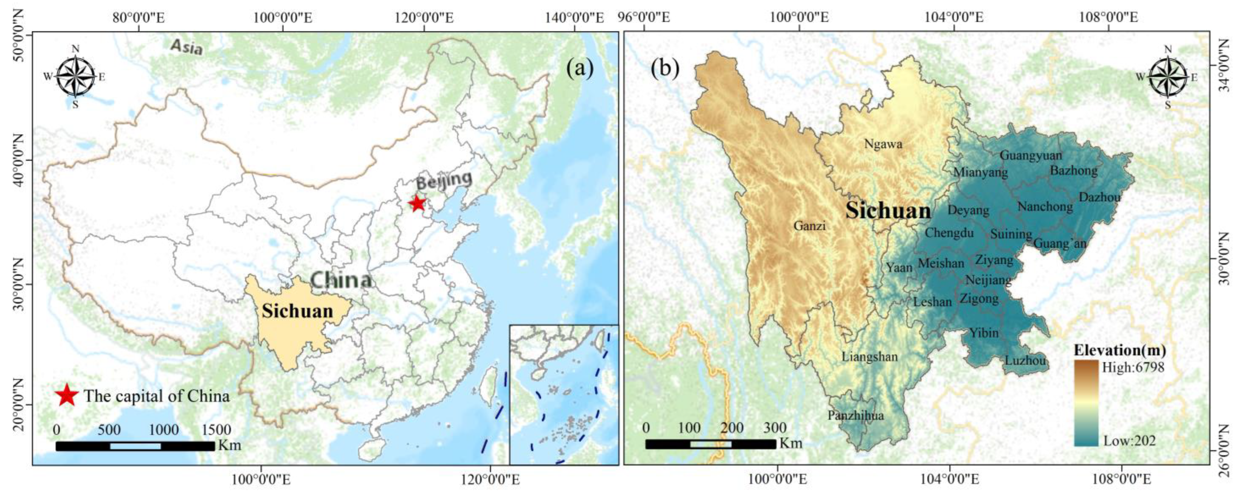
2. Study Area
3. Materials and Methods
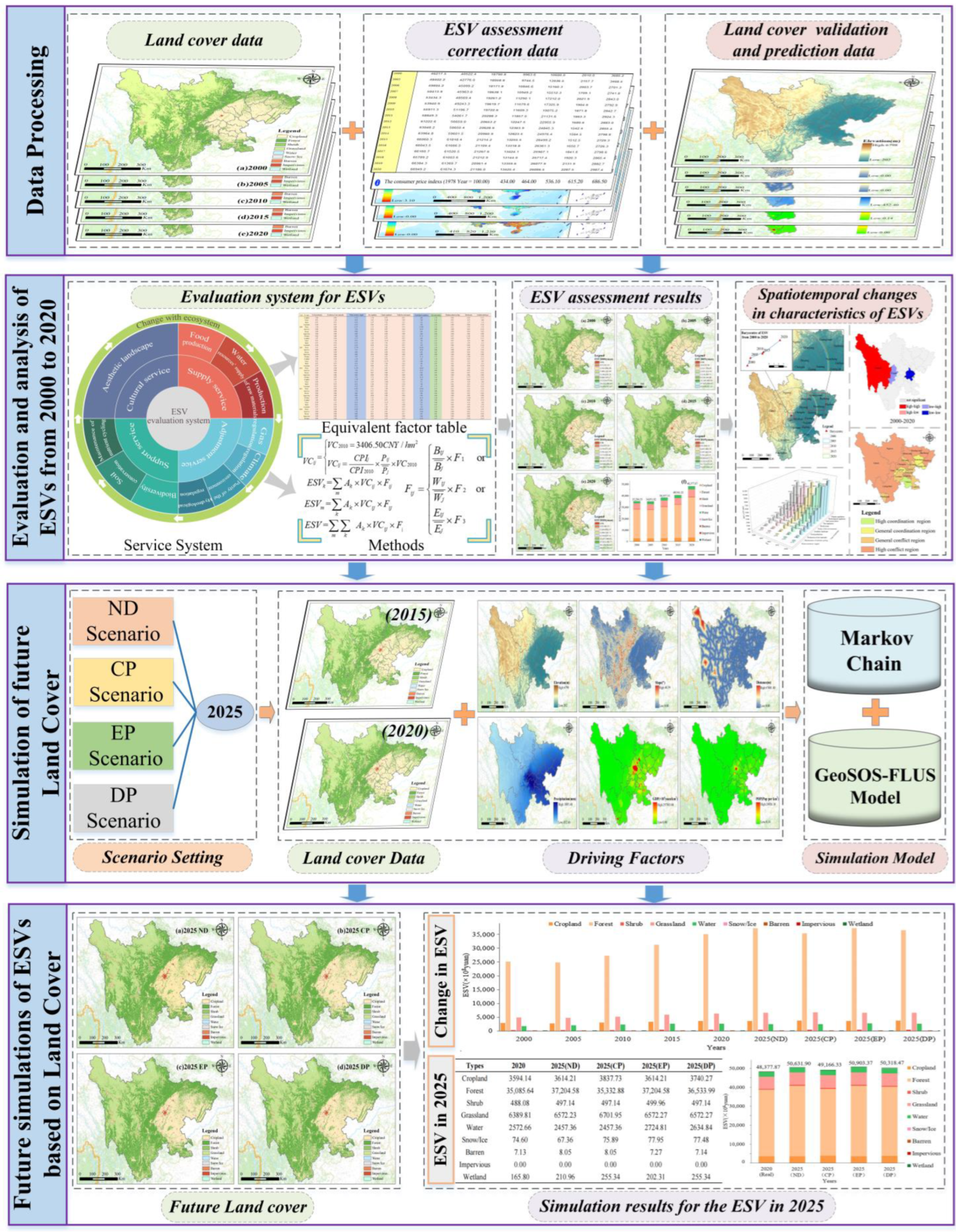
3.1. Framework Design
3.2. Data Source and Preprocess
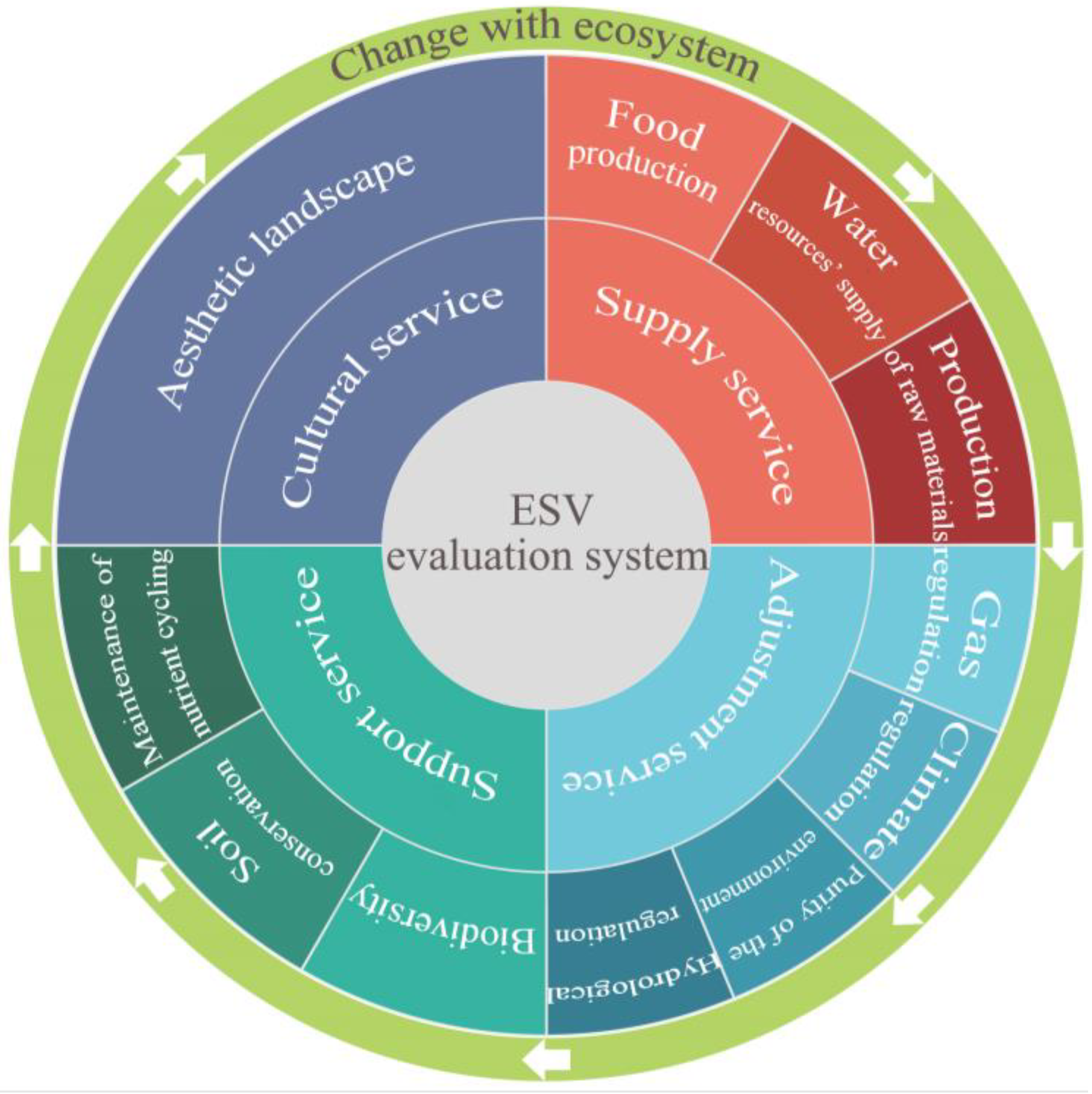
3.3. Evaluation Method of ESVs
3.3.1. Calculation of the Standard Unit Equivalent Factor Value
3.3.2. Revision of the ESV Equivalent Factor Table
3.3.3. Calculation of ESV
3.4. Analysis of the Evolution of the Characteristics of ESV
3.4.1. Analysis of the Evolution of the Characteristics of the ESV
3.4.2. Spatial Heterogeneity of the ESV
3.4.3. Coupled Analysis of ESV and Sustainable Development
3.5. Simulation of Future Land Cover
3.5.1. Markov Chain Model
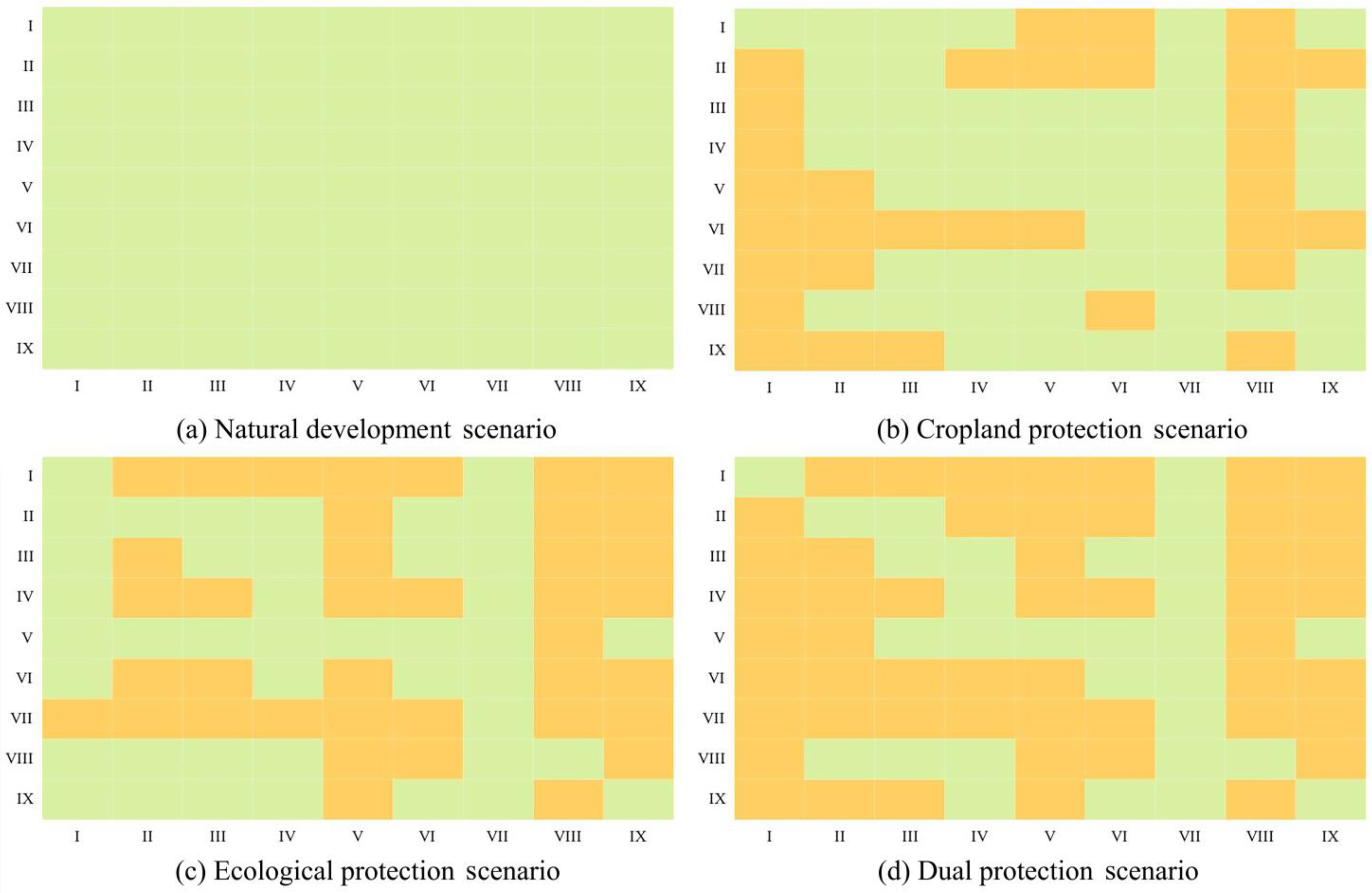
3.5.2. Scenario Setting
3.5.3. GeoSOS-FLUS Model
3.6. Model Validation
3.7. Future Simulations of ESVs Based on LC
4. Results and Analysis
4.1. Spatiotemporal Evolution of LC
4.1.1. Overall Characteristics of LC Changes
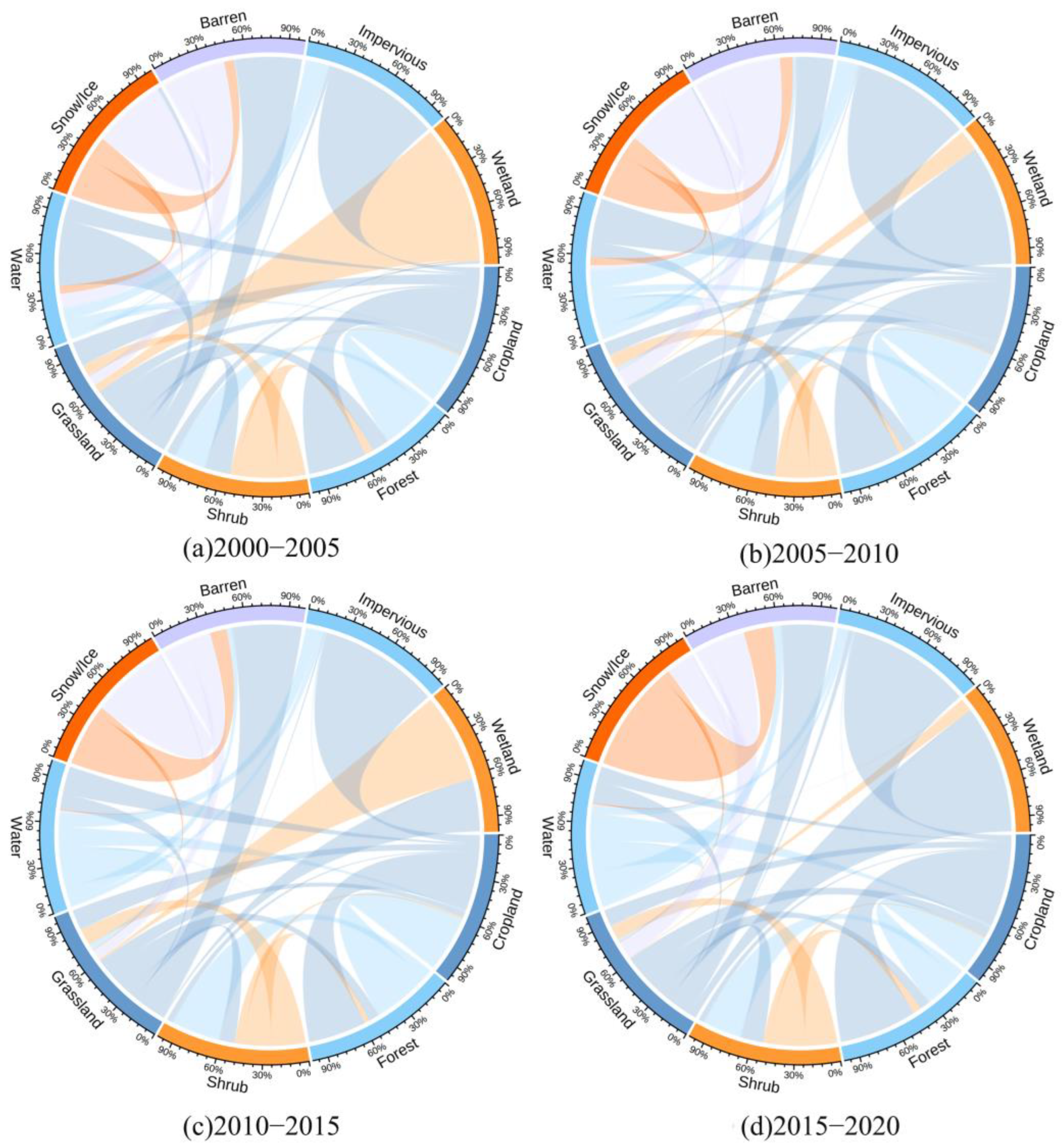
4.1.2. Structural Realignment Change in LC
4.2. Spatiotemporal Change in ESVs in Sichuan Province
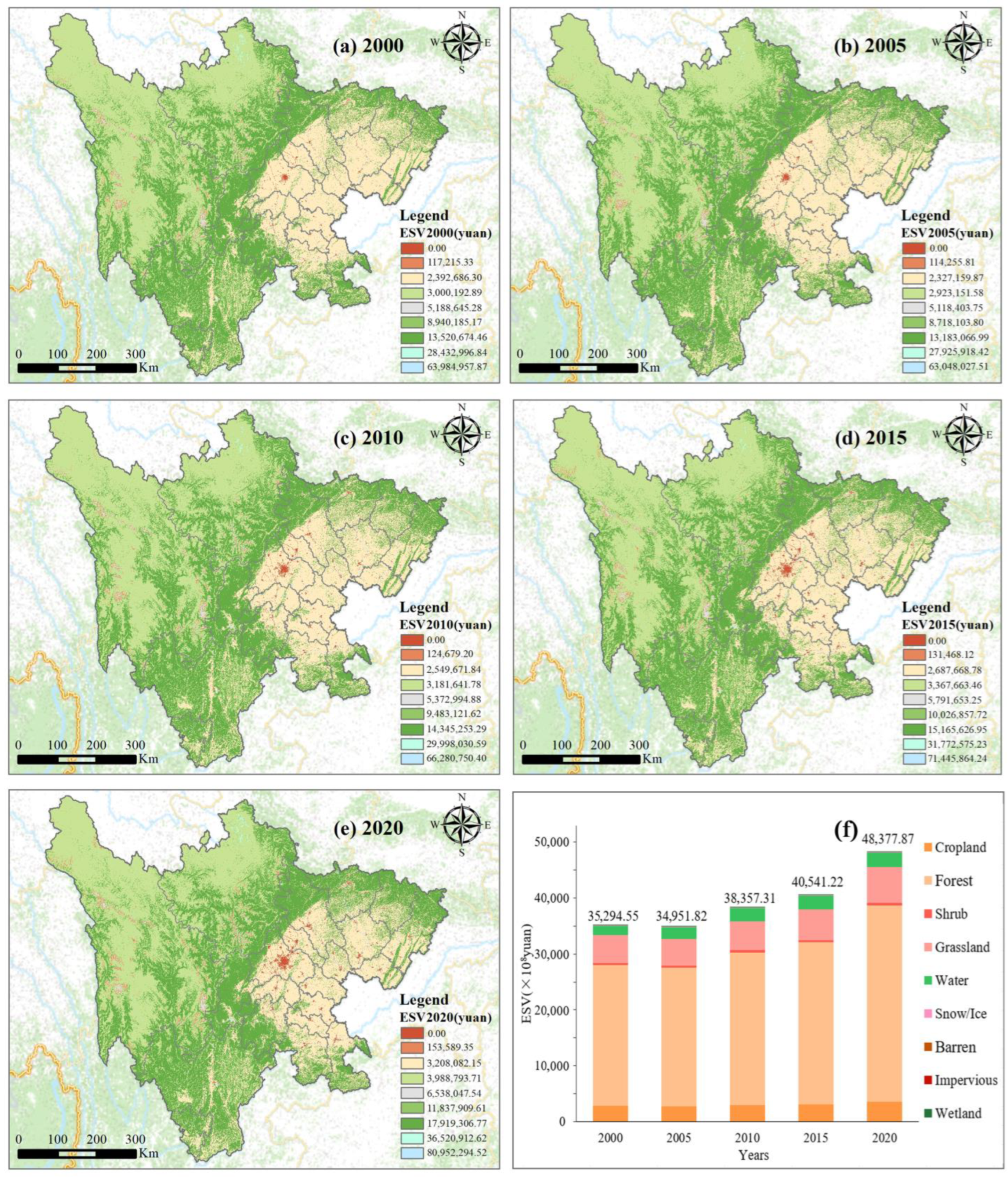
4.2.1. General Characteristics of Spatiotemporal Variations in ESVs
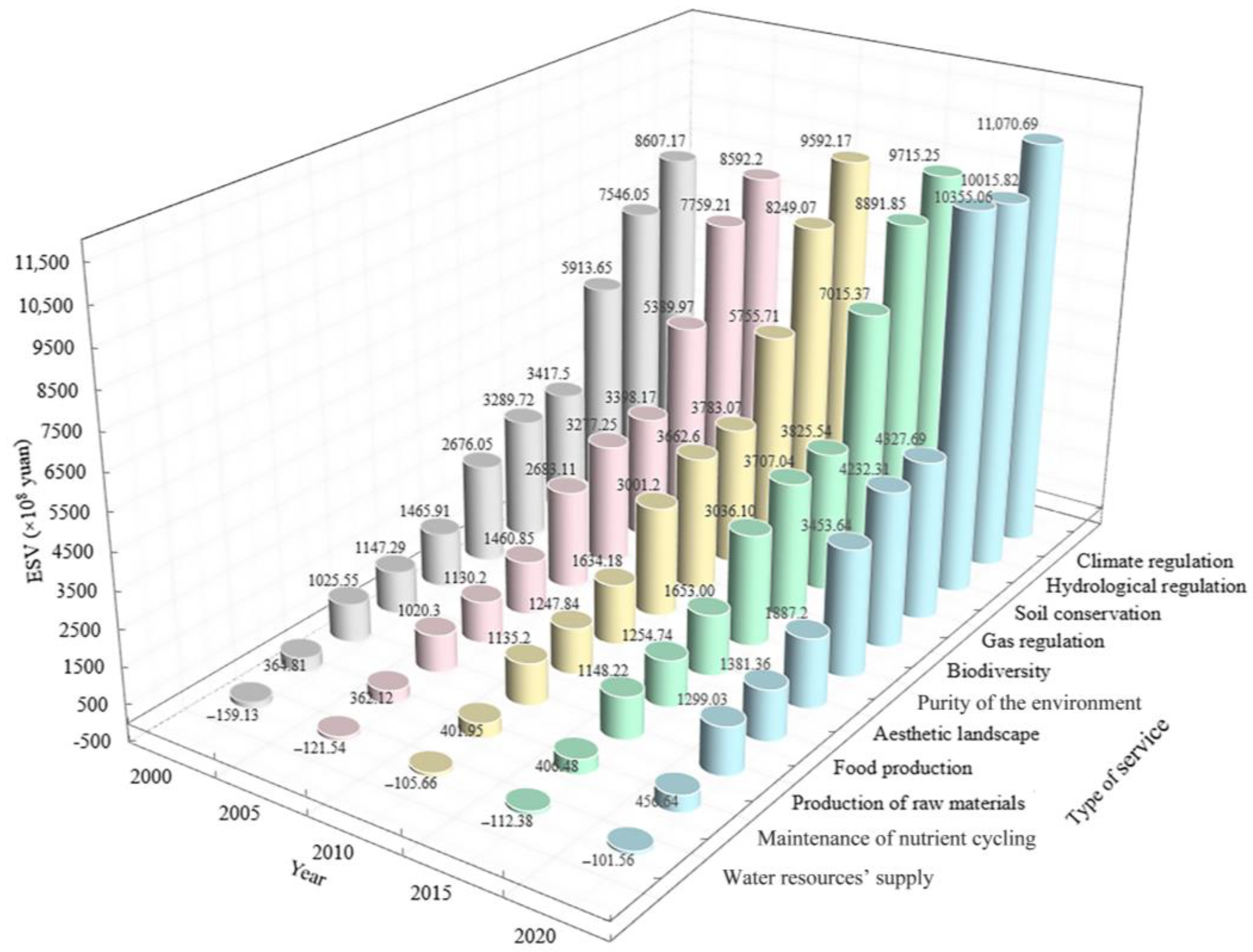
4.2.2. Analysis of Changes in ESV for Different Ecological Service Functions
4.2.3. Analysis of Changes in ESV in Prefecture-Level Cities
4.3. Multi-Scenario Simulation of LC and ESV
4.3.1. Validation of the GeoSOS-FLUS Model
4.3.2. Future LC modeling with Different Scenarios
4.3.3. ESV Assessment Based on Future LC Simulations
5. Discussion
5.1. Spatiotemporal Evolutionary Patterns of ESV and LC
5.2. Suitability of Multi-Scenario Simulation Results
5.3. ESV Evolution Driven by Policy Context
5.4. Limitations and Future Work
6. Conclusions
- (1)
- From 2000 to 2020, there was a consistent increase in the area of forests and impervious land, with forest cover expanding by 9748 km2. The most frequent transitions were observed between croplands, forests, and grasslands.
- (2)
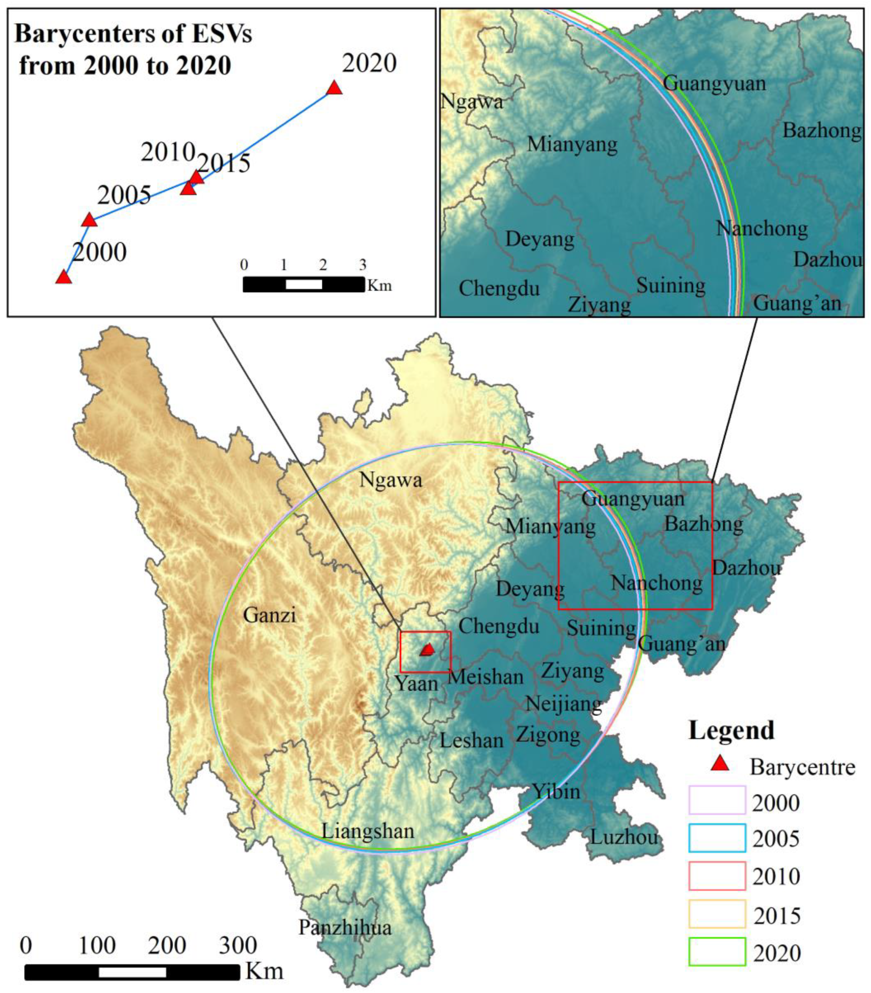
- The overall ESV remained relatively stable and exhibited a positive trend, with forests playing a significant role in this increase. The barycenter for ESV was found to be in the northeastern part of Ya’an, and it has been gradually shifting northeast since 2000. The ESV associated with the soil and water conservation function demonstrated remarkable performance, with a cumulative increase of 75% compared to that of 2000.
- (3)
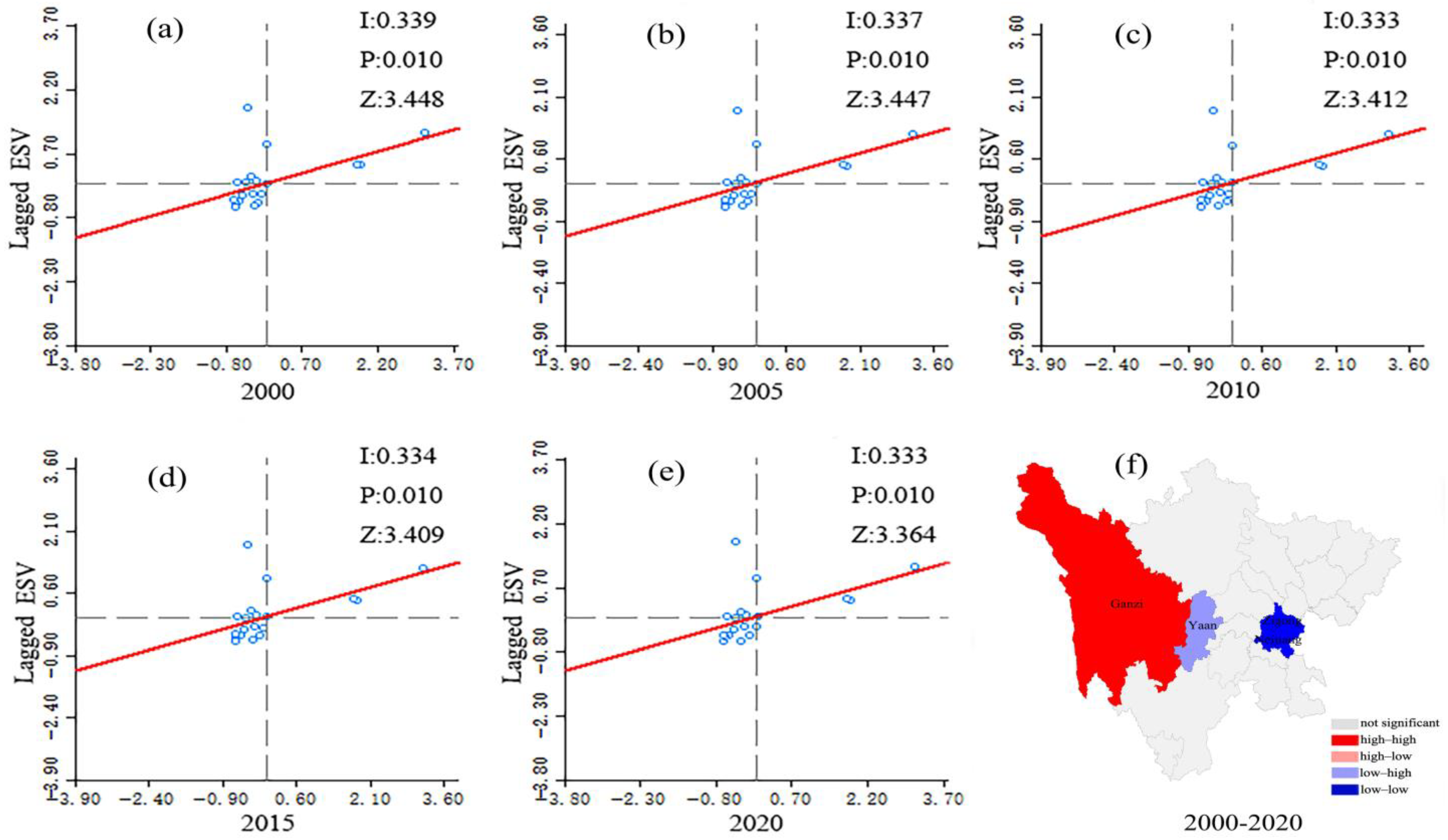
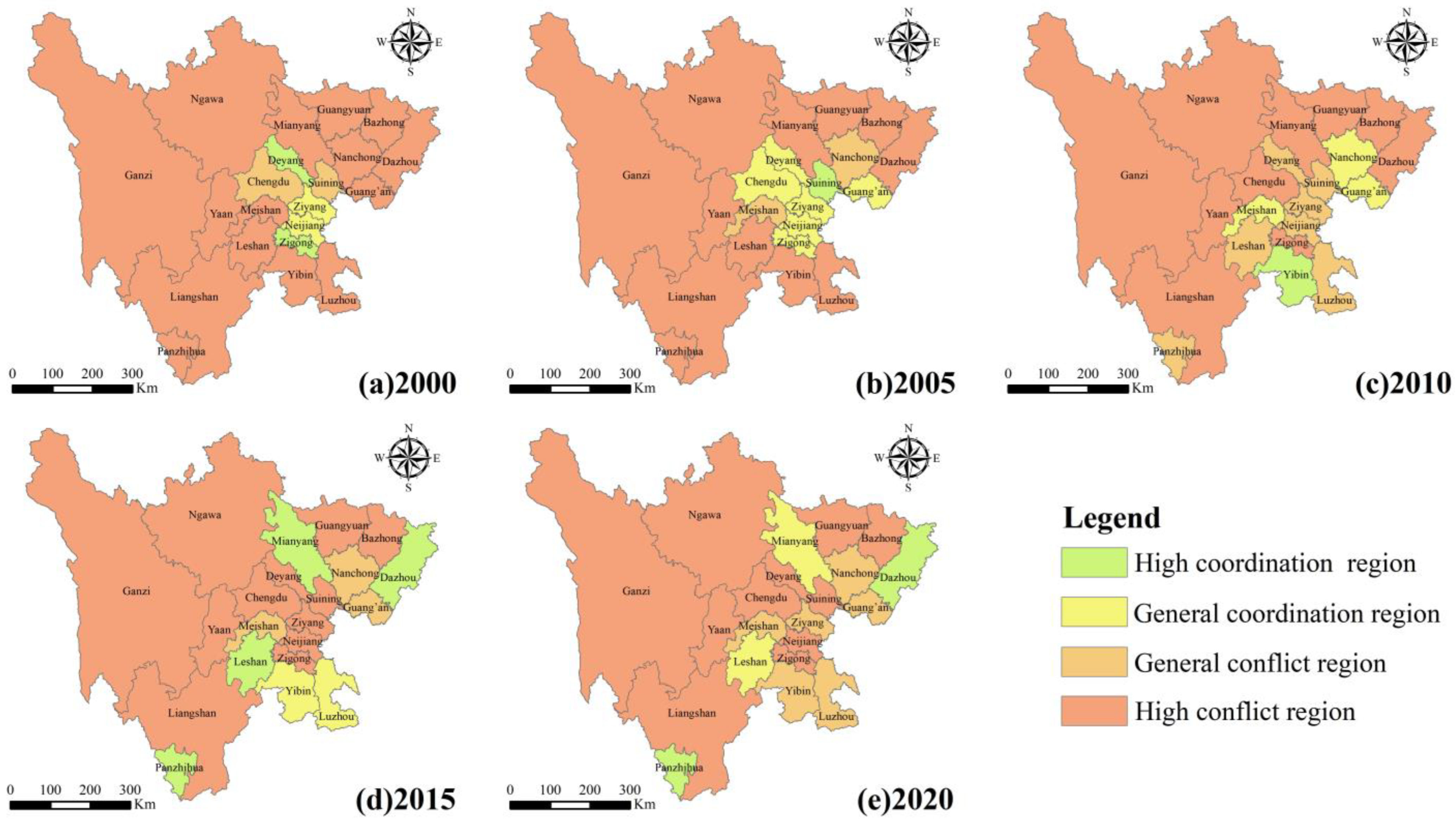
- The ESV aggregation pattern of each city has remained unchanged, with Ganzi being the only city with high aggregation. The degradation and imbalanced development in Zigong and Neijiang are constraining the improvement of the overall ESV. Overall, there are more conflict cities than coordination cities between economic development and the ecological environment. High conflict cities are concentrated in Ganzi, Ngawa, Liangshan, Yan, Bazhong, and Guangdong. Chengdu and its surrounding cities have gradually transitioned from coordination cities to conflict cities. The coordination in Panzhihua and Bazhong shows a continuous trend of improvement.
- (4)
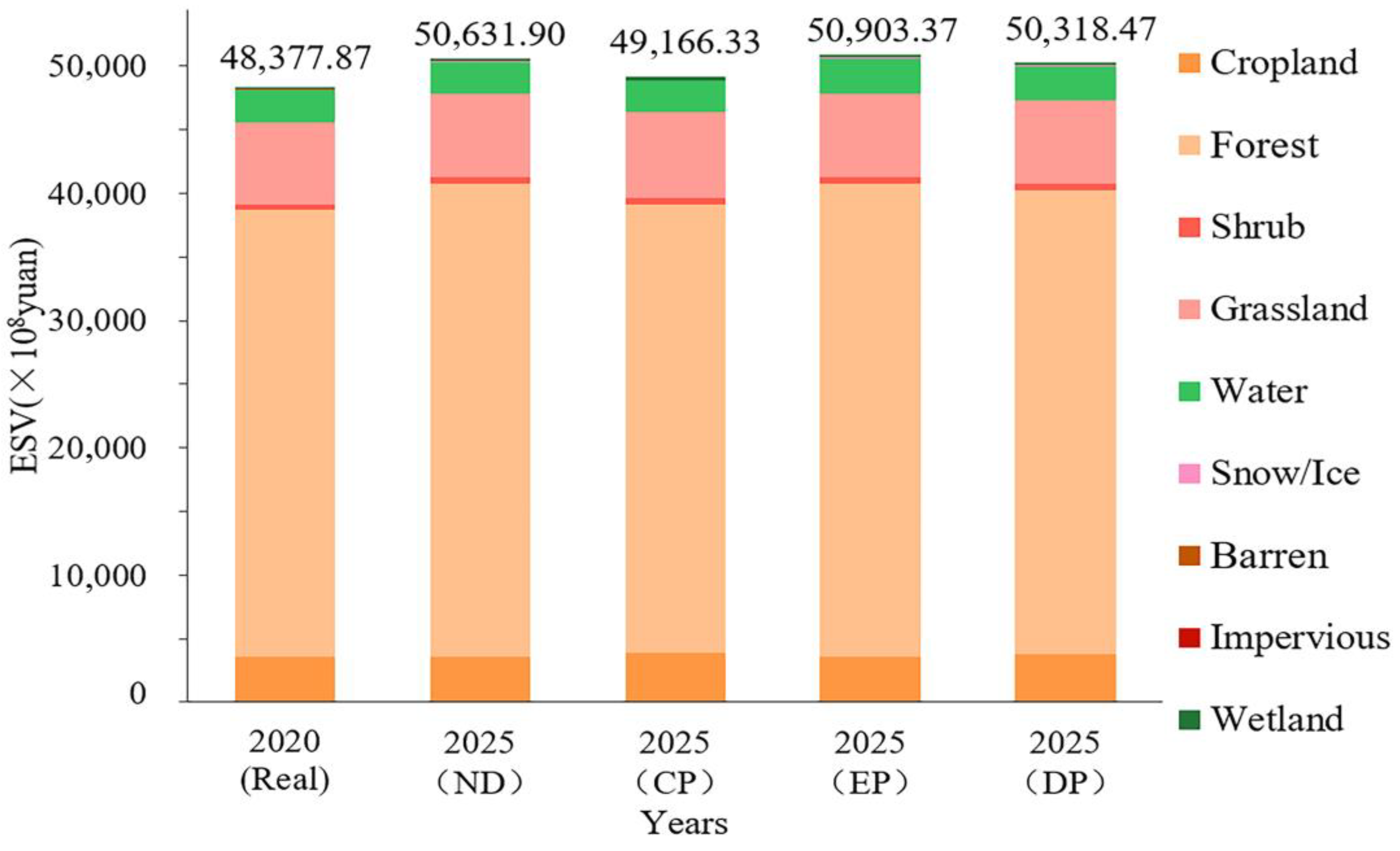
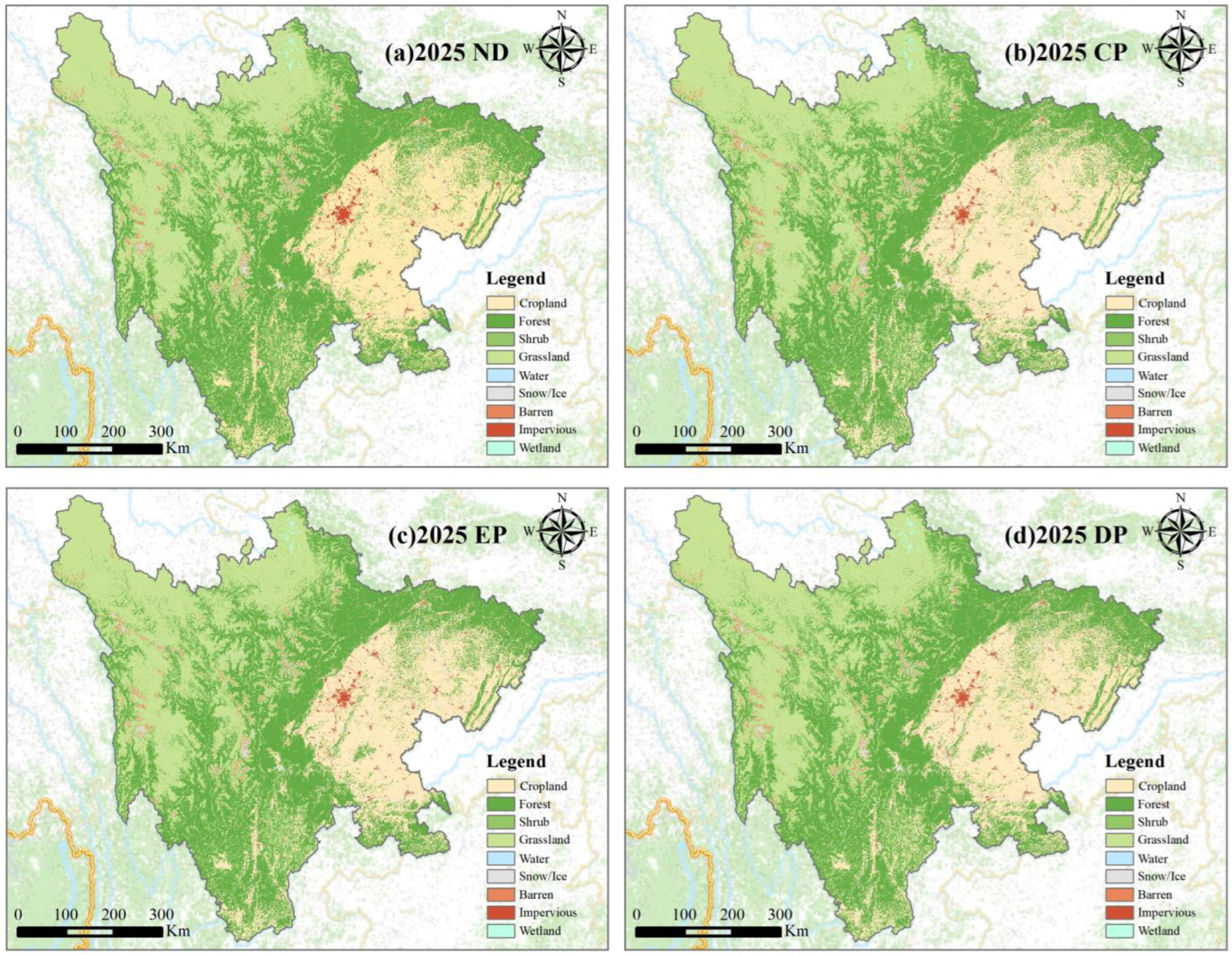
- Our simulation results align closely with the actual LC in 2020. Under all four development scenarios, the ESV of Sichuan Province in 2025 has increased, with the highest total ESV being that under the EP scenario that will reach 50,903.37 × 108 yuan.
Author Contributions
Funding
Data Availability Statement
Acknowledgments
Conflicts of Interest
Appendix A

| Ecosystem Services | Supply Service | Adjustment Service | Support Service | Cultural Service | ||||||||
|---|---|---|---|---|---|---|---|---|---|---|---|---|
| Food Production | Production of Raw Materials | Water Resources’ Supply | Gas Regulation | Climate Regulation | Purity of the Environment | Hydrological Regulation | Soil Conservation | Maintenance of Nutrient Cycling | Biodiversity | Aesthetic Landscape | ||
| 2000 | Cropland | 1.86 | 0.46 | −1.73 | 1.50 | 0.78 | 0.23 | 2.04 | 1.56 | 0.26 | 0.29 | 0.13 |
| Forest | 0.51 | 1.16 | 0.52 | 3.81 | 11.40 | 3.39 | 7.28 | 7.14 | 0.35 | 4.23 | 1.86 | |
| Shrub | 0.33 | 0.75 | 0.34 | 2.47 | 7.42 | 2.25 | 5.14 | 4.64 | 0.23 | 2.75 | 1.21 | |
| Grassland | 0.18 | 0.25 | 0.12 | 0.89 | 2.35 | 0.77 | 1.50 | 1.67 | 0.09 | 0.98 | 0.44 | |
| Water | 1.40 | 0.40 | 12.73 | 1.35 | 4.02 | 9.74 | 157.00 | 2.51 | 0.12 | 4.47 | 3.32 | |
| Snow/Ice | 0.00 | 0.00 | 3.32 | 0.32 | 0.95 | 0.28 | 10.95 | 0.00 | 0.00 | 0.02 | 0.16 | |
| Barren | 0.00 | 0.00 | 0.00 | 0.04 | 0.00 | 0.18 | 0.05 | 0.05 | 0.00 | 0.04 | 0.02 | |
| Impervious | 0.00 | 0.00 | 0.00 | 0.00 | 0.00 | 0.00 | 0.00 | 0.00 | 0.00 | 0.00 | 0.00 | |
| Wetland | 0.89 | 0.88 | 3.98 | 3.33 | 6.32 | 6.32 | 37.21 | 6.23 | 0.32 | 13.81 | 8.30 | |
| 2005 | Cropland | 1.87 | 0.46 | −1.73 | 1.50 | 0.79 | 0.23 | 2.03 | 1.43 | 0.26 | 0.29 | 0.13 |
| Forest | 0.51 | 1.16 | 0.52 | 3.81 | 11.43 | 3.39 | 7.26 | 6.55 | 0.35 | 4.24 | 1.86 | |
| Shrub | 0.33 | 0.76 | 0.34 | 2.48 | 7.44 | 2.25 | 5.13 | 4.25 | 0.23 | 2.76 | 1.21 | |
| Grassland | 0.18 | 0.25 | 0.12 | 0.90 | 2.36 | 0.77 | 1.50 | 1.53 | 0.09 | 0.98 | 0.44 | |
| Water | 1.41 | 0.40 | 12.70 | 1.35 | 4.03 | 9.76 | 156.58 | 2.30 | 0.12 | 4.48 | 3.32 | |
| Snow/Ice | 0.00 | 0.00 | 3.31 | 0.32 | 0.95 | 0.28 | 10.92 | 0.00 | 0.00 | 0.02 | 0.16 | |
| Barren | 0.00 | 0.00 | 0.00 | 0.04 | 0.00 | 0.18 | 0.05 | 0.05 | 0.00 | 0.04 | 0.02 | |
| Impervious | 0.00 | 0.00 | 0.00 | 0.00 | 0.00 | 0.00 | 0.00 | 0.00 | 0.00 | 0.00 | 0.00 | |
| Wetland | 0.90 | 0.88 | 3.97 | 3.34 | 6.33 | 6.33 | 37.11 | 5.71 | 0.32 | 13.83 | 8.31 | |
| 2010 | Cropland | 1.86 | 0.46 | −1.62 | 1.49 | 0.78 | 0.23 | 1.91 | 1.36 | 0.26 | 0.29 | 0.13 |
| Forest | 0.51 | 1.15 | 0.49 | 3.80 | 11.37 | 3.38 | 6.80 | 6.24 | 0.35 | 4.22 | 1.85 | |
| Shrub | 0.33 | 0.75 | 0.32 | 2.47 | 7.40 | 2.24 | 4.81 | 4.05 | 0.23 | 2.75 | 1.21 | |
| Grassland | 0.17 | 0.24 | 0.11 | 0.89 | 2.34 | 0.77 | 1.41 | 1.46 | 0.09 | 0.98 | 0.44 | |
| Water | 1.40 | 0.40 | 11.89 | 1.35 | 4.01 | 9.71 | 146.69 | 2.19 | 0.12 | 4.46 | 3.31 | |
| Snow/Ice | 0.00 | 0.00 | 3.10 | 0.31 | 0.94 | 0.28 | 10.23 | 0.00 | 0.00 | 0.02 | 0.16 | |
| Barren | 0.00 | 0.00 | 0.00 | 0.03 | 0.00 | 0.17 | 0.04 | 0.05 | 0.00 | 0.03 | 0.02 | |
| Impervious | 0.00 | 0.00 | 0.00 | 0.00 | 0.00 | 0.00 | 0.00 | 0.00 | 0.00 | 0.00 | 0.00 | |
| Wetland | 0.89 | 0.87 | 3.72 | 3.32 | 6.30 | 6.30 | 34.76 | 5.44 | 0.31 | 13.77 | 8.28 | |
| 2015 | Cropland | 1.81 | 0.45 | −1.69 | 1.45 | 0.76 | 0.22 | 1.99 | 1.60 | 0.25 | 0.28 | 0.12 |
| Forest | 0.49 | 1.12 | 0.51 | 3.69 | 11.06 | 3.29 | 7.11 | 7.32 | 0.34 | 4.10 | 1.80 | |
| Shrub | 0.32 | 0.73 | 0.33 | 2.40 | 7.20 | 2.18 | 5.02 | 4.75 | 0.22 | 2.67 | 1.17 | |
| Grassland | 0.17 | 0.24 | 0.12 | 0.87 | 2.28 | 0.75 | 1.47 | 1.71 | 0.09 | 0.95 | 0.43 | |
| Water | 1.36 | 0.39 | 12.43 | 1.31 | 3.90 | 9.45 | 153.30 | 2.57 | 0.12 | 4.34 | 3.22 | |
| Snow/Ice | 0.00 | 0.00 | 3.24 | 0.31 | 0.92 | 0.27 | 10.69 | 0.00 | 0.00 | 0.02 | 0.15 | |
| Barren | 0.00 | 0.00 | 0.00 | 0.03 | 0.00 | 0.17 | 0.04 | 0.06 | 0.00 | 0.03 | 0.02 | |
| Impervious | 0.00 | 0.00 | 0.00 | 0.00 | 0.00 | 0.00 | 0.00 | 0.00 | 0.00 | 0.00 | 0.00 | |
| Wetland | 0.87 | 0.85 | 3.88 | 3.23 | 6.13 | 6.13 | 36.33 | 6.38 | 0.31 | 13.40 | 8.05 | |
| 2020 | Cropland | 1.83 | 0.45 | −1.72 | 1.47 | 0.77 | 0.22 | 2.03 | 2.09 | 0.26 | 0.28 | 0.12 |
| Forest | 0.50 | 1.13 | 0.52 | 3.73 | 11.17 | 3.32 | 7.24 | 9.60 | 0.34 | 4.14 | 1.82 | |
| Shrub | 0.33 | 0.74 | 0.34 | 2.42 | 7.27 | 2.20 | 5.12 | 6.23 | 0.22 | 2.70 | 1.19 | |
| Grassland | 0.17 | 0.24 | 0.12 | 0.88 | 2.30 | 0.76 | 1.50 | 2.25 | 0.09 | 0.96 | 0.43 | |
| Water | 1.37 | 0.40 | 12.67 | 1.32 | 3.94 | 9.54 | 156.25 | 3.37 | 0.12 | 4.38 | 3.25 | |
| Snow/Ice | 0.00 | 0.00 | 3.30 | 0.31 | 0.93 | 0.27 | 10.90 | 0.00 | 0.00 | 0.02 | 0.15 | |
| Barren | 0.00 | 0.00 | 0.00 | 0.03 | 0.00 | 0.17 | 0.05 | 0.07 | 0.00 | 0.03 | 0.02 | |
| Impervious | 0.00 | 0.00 | 0.00 | 0.00 | 0.00 | 0.00 | 0.00 | 0.00 | 0.00 | 0.00 | 0.00 | |
| Wetland | 0.88 | 0.86 | 3.96 | 3.27 | 6.19 | 6.19 | 37.03 | 8.37 | 0.31 | 13.53 | 8.13 | |
References
- Desta, H. Local perceptions of ecosystem services and human-induced degradation of lake Ziway in the Rift Valley region of Ethiopia. Ecol. Indic. 2021, 127, 107786. [Google Scholar] [CrossRef]
- Escobedo, F.J.; Kroeger, T.; Wagner, J.E. Urban forests and pollution mitigation: Analyzing ecosystem services and disservices. Environ. Pollut. 2011, 159, 2078–2087. [Google Scholar] [CrossRef] [PubMed]
- Baral, H.; Keenan, R.J.; Sharma, S.K.; Stork, N.E.; Kasel, S. Economic evaluation of ecosystem goods and services under different landscape management scenarios. Land Use Policy 2014, 39, 54–64. [Google Scholar] [CrossRef]
- Chen, S.; Li, G.; Xu, Z.; Zhuo, Y.; Wu, C.; Ye, Y. Combined Impact of Socioeconomic Forces and Policy Implications: Spatial-Temporal Dynamics of the Ecosystem Services Value in Yangtze River Delta, China. Sustainability 2019, 11, 2622. [Google Scholar] [CrossRef]
- Ping, Z.; Liang, H.; Xin, F.; Peishu, H.; Yunhui, L.; Tao, Z.; Ying, P.; Zhenrong, Y. Ecosystem Service Value Assessment and Contribution Factor Analysis of Land Use Change in Miyun County, China. Sustainability 2015, 7, 7333. [Google Scholar] [CrossRef]
- De Groot, R.; Brander, L.; Van Der Ploeg, S.; Costanza, R.; Bernard, F.; Braat, L.; Christie, M.; Crossman, N.; Ghermandi, A.; Hein, L.; et al. Global estimates of the value of ecosystems and their services in monetary unit. Ecosyst. Serv. 2012, 1, 50–61. [Google Scholar] [CrossRef]
- Costanza, R.; de Groot, R.; Sutton, P.; van der Ploeg, S.; Anderson, S.J.; Kubiszewski, I.; Farber, S.; Turner, R.K. Changes in the global value of ecosystem services. Glob. Environ. Change 2014, 26, 152–158. [Google Scholar] [CrossRef]
- Xie, G.; Zhang, C.; Zhen, L.; Zhang, L. Dynamic changes in the value of China’s ecosystem services. Ecosyst. Serv. 2017, 26, 146–154. [Google Scholar] [CrossRef]
- Zhao, H.; Xu, X.; Tang, J.; Wang, Z.; Miao, C. Understanding the key factors and future trends of ecosystem service value to support the decision management in the cluster cities around the Yellow River floodplain area. Ecol. Indic. 2023, 154, 110544. [Google Scholar] [CrossRef]
- Wang, X.; Pan, T.; Pan, R.; Chi, W.; Ma, C.; Ning, L.; Wang, X.; Zhang, J. Impact of Land Transition on Landscape and Ecosystem Service Value in Northeast Region of China from 2000–2020. Land 2022, 11, 696. [Google Scholar] [CrossRef]
- Xie, G.; Zhang, C.; Zhang, C.; Xiao, Y. The value of ecosystem services in China. Resour. Sci. 2015, 30, 1243–1252. [Google Scholar]
- Zhao, T.; Ouyang, Z.; Jia, L.; Zheng, H. Ecosystem services and their valuation of China grassland. Acta Geogr. Sin. 2004, 24, 1101–1110. [Google Scholar]
- Wang, B.; Lu, S. Evaluation of economic forest ecosystem services in China. J. Appl. Ecol. 2009, 20, 417–425. [Google Scholar]
- Sun, J. Research Advances and Trends in Ecosystem Services and Evaluation in China. Procedia Environ. Sci. 2011, 2011, 1791–1796. [Google Scholar]
- Chen, D.; Zhong, L. Review of the value evaluation and realization mechanism of ecosystem services. Chin. J. Agric. Resour. Reg. Plan. 2023, 44, 84–94. [Google Scholar]
- Costanza, R.; Darge, R.; Groot, R.; Belt, H. The value of the world’s ecosystem services and natural capital. Nature 1997, 387, 253–260. [Google Scholar] [CrossRef]
- Duan, X.Y.; Chen, Y.; Wang, L.Q.; Zheng, G.D.; Liang, T. The impact of land use and land cover changes on the landscape pattern and ecosystem service value in Sanjiangyuan region of the Qinghai-Tibet Plateau. J. Environ. Manag. 2023, 325, 10. [Google Scholar] [CrossRef] [PubMed]
- Huang, Z.; Chen, Y.; Zheng, Z.; Wu, Z. Spatiotemporal coupling analysis between human footprint and ecosystem service value in the highly urbanized Pearl River Delta urban Agglomeration, China. Ecol. Indic. 2023, 148, 110033. [Google Scholar] [CrossRef]
- Burkhard, B.; Müller, A.; Müller, F.; Grescho, V.; Anh, Q.; Arida, G.; Bustamante, J.V.; Van Chien, H.; Heong, K.L.; Escalada, M.; et al. Land cover-based ecosystem service assessment of irrigated rice cropping systems in southeast Asia—An explorative study. Ecosyst. Serv. 2015, 14, 76–87. [Google Scholar] [CrossRef]
- Xiao, Y.; Huang, M.; Xie, G.; Zhen, L. Evaluating the impacts of land use change on ecosystem service values under multiple scenarios in the Hunshandake region of China. Sci. Total Environ. 2022, 850, 158067. [Google Scholar] [CrossRef]
- Rahman, M.M.; Szabó, G. Impact of Land Use and Land Cover Changes on Urban Ecosystem Service Value in Dhaka, Bangladesh. Land 2021, 10, 793. [Google Scholar] [CrossRef]
- Polasky, S.; Nelson, E.; Pennington, D.; Johnson, K.A. The Impact of Land-Use Change on Ecosystem Services, Biodiversity and Returns to Landowners: A Case Study in the State of Minnesota. Environ. Resour. Econ. 2011, 48, 219–242. [Google Scholar] [CrossRef]
- Yi, H.; Gueneralp, B.; Filippi, A.M.; Kreuter, U.P.; Gueneralp, I. Impacts of Land Change on Ecosystem Services in the San Antonio River Basin, Texas, from 1984 to 2010. Ecol. Econ. 2017, 135, 125–135. [Google Scholar] [CrossRef]
- Ávila-García, D.; Morató, J.; Pérez-Maussán, A.I.; Santillán-Carvantes, P.; Alvarado, J.; Comín, F.A. Impacts of alternative land-use policies on water ecosystem services in the Río Grande de Comitán-Lagos de Montebello watershed, Mexico. Ecosyst. Serv. 2020, 45, 101179. [Google Scholar] [CrossRef]
- Batty, M.; Couclelis, H.; Eichen, M. Urban Systems as Cellular Automata. Environ. Plan. B Plan. Des. 1997, 24, 159–164. [Google Scholar] [CrossRef]
- Nehzak, H.K.; Aghaei, M.; Mostafazadeh, R.; Dastjerdi, R. Evaluation of land use change predictions using CA-Markov model and management scenarios. Comput. Earth Environ. Sci. 2022, 6, 105–115. [Google Scholar]
- e Silva, L.P.; Xavier, A.P.C.; da Silva, R.M.; Santos, C.A.G. Modeling land cover change based on an artificial neural network for a semiarid river basin in northeastern Brazil. Glob. Ecol. Conserv. 2019, 21, 811–825. [Google Scholar] [CrossRef]
- Verburg, P.H.; Soepboer, W.; Veldkamp, A. Modeling the Spatial Dynamics of Regional Land Use: The CLUE-S Model. Environ. Manag. 2002, 30, 391. [Google Scholar] [CrossRef]
- Liu, X.; Liang, X.; Li, X.; Xu, X.; Wang, S. A future land use simulation model (FLUS) for simulating multiple land use scenarios by coupling human and natural effects. Landsc. Urban Plan. 2017, 168, 94–116. [Google Scholar] [CrossRef]
- Meng, F.; Guo, J.; Guo, Z.; Lee, J.C.K.; Liu, G.; Wang, N. Urban ecological transition: The practice of ecological civilization construction in China. Sci. Total Environ. 2021, 755, 142633–142643. [Google Scholar] [CrossRef]
- Zhang, X.; Wang, Y.; Qi, Y.; Wu, J.; Liao, W.; Shui, W.; Zhang, Y.; Deng, S.; Peng, H.; Yu, X. Evaluating the trends of China’s ecological civilization construction using a novel indicator system. J. Clean. Prod. 2016, 133, 910–923. [Google Scholar] [CrossRef]
- Wei, X.Y.; Xia, J.X. Ecological compensation for large water projects based on ecological footprint theory: A case study in China. Procedia Environ. Sci. 2012, 13, 1338–1345. [Google Scholar] [CrossRef]
- Qin, Y.; Yan, H.; Liu, J.; Dong, J.; Chen, J.; Xiao, X. Impacts of ecological restoration projects on agricultural productivity in China. Chin. Geogr. Lsci. 2013, 23, 404–416. [Google Scholar] [CrossRef]
- Zhang, G.; Dong, J.; Xiao, X.; Hu, Z.; Sheldon, S. Effectiveness of ecological restoration projects in Horqin Sandy Land, China based on SPOT-VGT NDVI data. Ecol. Eng. 2012, 38, 20–29. [Google Scholar] [CrossRef]
- Shao, Q.; Liu, S.; Ning, J.; Liu, G.; Yang, F. Assessment of ecological benefits of key national ecological projects in China in 2000–2019 using remote sensing. Acta Geogr. Sin. 2022, 77, 2133–2153. [Google Scholar]
- Chu, X.; Zhan, J.; Li, Z.; Zhang, F.; Qi, W. Assessment on forest carbon sequestration in the Three-North Shelterbelt Program region, China. J. Clean. Prod. 2019, 215, 382–389. [Google Scholar] [CrossRef]
- Zhou, D.; Zhao, S.; Zhu, C. The Grain for Green Project induced land cover change in the Loess Plateau: A case study with Ansai County, Shanxi Province, China. Ecol. Indic. 2012, 23, 88–94. [Google Scholar] [CrossRef]
- Wei, X.; Zhao, L.; Cheng, P.; Xie, M.; Wang, H. Spatial-Temporal Dynamic Evaluation of Ecosystem Service Value and Its Driving Mechanisms in China. Land 2022, 11, 1000. [Google Scholar] [CrossRef]
- Han, R.; Sun, S.; Guo, L.; Chen, Y. Evolution of Ecosystem Service Value and Analysis of Driving Forces in the East Region of Sichuan Province, China. J. Ecol. Rural Environ. 2019, 35, 1136–1143. [Google Scholar]
- Jiang, Z.; Gan, X.; Liu, J.; Bi, X.; Kang, A.; Zhou, B. Landscape Ecological Risk Assessment and Zoning Control Based on Ecosystem Service Value: Taking Sichuan Province as an Example. Appl. Sci. 2023, 13, 12103. [Google Scholar] [CrossRef]
- Cai, H.; Yang, X.; Xu, X. Human-induced grassland degradation/restoration in the central Tibetan Plateau: The effects of ecological protection and restoration projects. Ecol. Eng. 2015, 83, 112–119. [Google Scholar] [CrossRef]
- Zhao, M.; He, Z. Evaluation of the Effects of Land Cover Change on Ecosystem Service Values in the Upper Reaches of the Heihe River Basin, Northwestern China. Sustainability 2018, 10, 4700. [Google Scholar] [CrossRef]
- Huang, K.; Deng, X.; Liu, Y.; Yong, Z.; Xu, D. Does off-Farm Migration of Female Laborers Inhibit Land Transfer? Evidence from Sichuan Province, China. Land 2020, 9, 14. [Google Scholar] [CrossRef]
- Xiong, K.; Adhikari, B.R.; Stamatopoulos, C.A.; Zhan, Y.; Di, B. Comparison of Different Machine Learning Methods for Debris Flow Susceptibility Mapping: A Case Study in the Sichuan Province, China. Remote Sens. 2020, 12, 295. [Google Scholar] [CrossRef]
- He, R.; Huang, X.T.; Ye, X.Y.; Pan, Z.; Wang, H.; Luo, B.; Liu, D.M.; Hu, X.X. County Ecosystem Health Assessment Based on the VORS Model: A Case Study of 183 Counties in Sichuan Province, China. Sustainability 2022, 14, 11565. [Google Scholar] [CrossRef]
- Peng, W.F.; Kuang, T.T.; Tao, S. Quantifying influences of natural factors on vegetation NDVI changes based on geographical detector in Sichuan, western China. J. Clean. Prod. 2019, 233, 353–367. [Google Scholar] [CrossRef]
- Yang, J.; Huang, X. The 30 m annual land cover dataset and its dynamics in China from 1990 to 2019. Earth Syst. Sci. Data 2021, 13, 3907–3925. [Google Scholar] [CrossRef]
- Liu, J.; Xiong, J.; Chen, Y.; Sun, H.; Zhao, X.; Tu, F.; Gu, Y. An integrated model chain for future flood risk prediction under land-use changes. J. Environ. Manag. 2023, 342, 118125. [Google Scholar] [CrossRef]
- Ma, R.; Zhou, W.; Ren, J.; Huang, Y.; Wang, H. Multi-scenario simulation and optimization control of ecological security based on GeoSOS-FLUS model in ecological fragile area in northeast Qinghai-Tibet Plateau, China. Ecol. Indic. 2023, 151, 110324–110337. [Google Scholar] [CrossRef]
- Li, S.; Zhu, C.; Lin, Y. Conflicts between agricultural and ecological functions and their driving mechanisms in agroforestry ecotone areas from the perspective of land use functions. J. Clean. Prod. 2021, 317, 128453. [Google Scholar] [CrossRef]
- Cumming, G.S.; Buerkert, A.; Hoffmann, E.M.; Schlecht, E.; Cramon-Taubadel, S.V.; Tscharntke, T. Implications of agricultural transitions and urbanization for ecosystem services. Nature 2014, 515, 50–57. [Google Scholar] [CrossRef]
- Xiong, J.; Li, W.; Zhang, H.; Cheng, W.; Ye, C.; Zhao, Y. Selected Environmental Assessment Model and Spatial Analysis Method to Explain Correlations in Environmental and Socio-Economic Data with Possible Application for Explaining the State of the Ecosystem. Sustainability 2019, 11, 4781. [Google Scholar] [CrossRef]
- Gong, J.X. Clarifying the standard deviational ellipse. Geogr. Anal. 2002, 34, 155–167. [Google Scholar] [CrossRef]
- Zhao, Y.B.; Chen, R.Y.; Zang, P.; Huang, L.Q.; Ma, S.F.; Wang, S.J. Spatiotemporal patterns of global carbon intensities and their driving forces. Sci. Total Environ. 2022, 818, 151690. [Google Scholar] [CrossRef]
- Xia, N.; Hai, W.; Tang, M.; Song, J.; Quan, W.; Zhang, B.; Ma, Y. Spatiotemporal evolution law and driving mechanism of production–living–ecological space from 2000 to 2020 in Xinjiang, China. Ecol. Indic. 2023, 154, 110807. [Google Scholar] [CrossRef]
- Wei, W.; Peiji, S.; Xiaoxu, W.; Junju, Z.; Binbin, X. Evaluation of the coordinated development of economy and eco-environmental systems and spatial evolution in China. Acta Ecol. Sin. 2018, 38, 2636–2648. [Google Scholar]
- Ghosh, P.; Mukhopadhyay, A.; Chanda, A.; Mondal, P.; Akhand, A.; Mukherjee, S.; Nayak, S.K.; Ghosh, S.; Mitra, D.; Ghosh, T. Application of Cellular automata and Markov-chain model in geospatial environmental modeling—A review. Remote Sens. Appl. Soc. Environ. 2017, 5, 64–77. [Google Scholar] [CrossRef]
- Huang, Y.; Nian, P.; Zhang, W. The prediction of interregional land use differences in Beijing: A Markov model. Environ. Earth Sci. 2015, 73, 4077–4090. [Google Scholar] [CrossRef]
- Sanchayeeta, A.; Jane, S. Simulating Forest Cover Changes of Bannerghatta National Park Based on a CA-Markov Model: A Remote Sensing Approach. Remote Sens. 2012, 4, 3215–3243. [Google Scholar] [CrossRef]
- Liu, X.; Wei, M.; Li, Z.; Zeng, J. Multi-scenario simulation of urban growth boundaries with an ESP-FLUS model: A case study of the Min Delta region, China. Ecol. Indic. 2022, 135, 108538–108552. [Google Scholar] [CrossRef]
- Wang, J.; Lv, J.; Zhang, W.; Chen, T.; Yang, Y.; Wu, J. Land-Use Pattern Evaluation Using GeoSOS-FLUS in National Territory Spatial Planning: A Case Study of Changzhi City, Shanxi Province. Sustainability 2022, 14, 13752. [Google Scholar] [CrossRef]
- Wang, Y.; Shen, J.; Yan, W.; Chen, C. Backcasting approach with multi-scenario simulation for assessing effects of land use policy using GeoSOS-FLUS software. MethodsX 2019, 6, 1384–1397. [Google Scholar] [CrossRef]
- Khozani, Z.S.; Banadkooki, F.B.; Ehteram, M.; Ahmed, A.N.; El-Shafie, A. Combining autoregressive integrated moving average with Long Short-Term Memory neural network and optimisation algorithms for predicting ground water level. J. Clean. Prod. 2022, 348, 131224. [Google Scholar] [CrossRef]
- Li, S.; Bing, Z.; Jin, G. Spatially Explicit Mapping of Soil Conservation Service in Monetary Units Due to Land Use/Cover Change for the Three Gorges Reservoir Area, China. Remote Sens. 2019, 11, 468. [Google Scholar] [CrossRef]
- Chen, D.; Li, W.; Cai, X.; Jing, N.; Wang, R.; Tang, M.; Gao, Y. Analysis on the dynamic changes and their influencing factors of forest resources in Sichuan Province. J. Earth Environ. 2021, 12, 425–435. [Google Scholar]
- Zhang, D.; Dong, H. Understanding Arable Land Change Patterns and Driving Forces in Major Grain-Producing Areas: A Case Study of Sichuan Province Using the PLUS Model. Land 2023, 12, 1443. [Google Scholar] [CrossRef]
- Lai, J.; Yang, W. Dynamic changes of vegetation cover in natural forest area of western Sichuan in recent 29 years based on RS. Remote Sens. Land Resour. 2018, 30, 132–138. [Google Scholar]
- Ye, S.; Song, C.; Shen, S.; Gao, P.; Zhu, D. Spatial pattern of arable land-use intensity in China. Land Use Policy 2020, 99, 104845. [Google Scholar] [CrossRef]
- Wang, Z.; Wang, Z.; Zhang, B.; Lu, C.; Ren, C. Impact of land use/land cover changes on ecosystem services in the Nenjiang River Basin, Northeast China. Ecol. Process. 2015, 4, 13717–13729. [Google Scholar] [CrossRef]
- Liu, L.; Chen, Y.Y.; Wu, T.; Li, H.M. The drivers of air pollution in the development of western China: The case of Sichuan province. J. Clean. Prod. 2018, 197, 1169–1176. [Google Scholar] [CrossRef]
- Liang, X.Y.; Jin, X.B.; Liu, J.; Yin, Y.X.; Gu, Z.M.; Zhang, J.Y.; Zhou, Y.K. Formation mechanism and sustainable productivity impacts of non-grain croplands: Evidence from Sichuan Province, China. Land Degrad. Dev. 2023, 34, 1120–1132. [Google Scholar] [CrossRef]
- Huang, K.X.; Peng, L.; Wang, X.H.; Deng, W. Integrating circuit theory and landscape pattern index to identify and optimize ecological networks: A case study of the Sichuan Basin, China. Environ. Sci. Pollut. Res. 2022, 29, 66874–66887. [Google Scholar] [CrossRef] [PubMed]
- Shan, X.; Yin, J.; Wang, J. Risk assessment of shanghai extreme flooding under the land use change scenario. Nat. Hazards 2021, 110, 1039–1060. [Google Scholar] [CrossRef]
- Huang, C.B.; Zhao, D.Y.; Liu, C.; Liao, Q.P. Integrating territorial pattern and socioeconomic development into ecosystem service value assessment. Environ. Impact Assess. Rev. 2023, 100, 107088. [Google Scholar] [CrossRef]
- Tao, Y.; Lv, Y.; Li, F.; Hu, J.; Zhang, K.; Li, T.; Ren, Y. Assessment of Ecological Effect of the Natural Forest Protection Project in Southwest China. J. Ecol. Rural. Environ. 2016, 32, 716–723. [Google Scholar]
- Anley, M.A.; Minale, A.S.; Haregeweyn, N.; Gashaw, T. Assessing the impacts of land use/cover changes on ecosystem service values in Rib watershed, Upper Blue Nile Basin, Ethiopia. Trees For. People 2022, 7, 100212. [Google Scholar] [CrossRef]
- Xie, L.; Wang, H.; Liu, S. The ecosystem service values simulation and driving force analysis based on land use/land cover: A case study in inland rivers in arid areas of the Aksu River Basin, China. Ecol. Indic. 2022, 138, 108828. [Google Scholar] [CrossRef]
- Chen, W.; Wang, G.; Zeng, J. Impact of urbanization on ecosystem health in Chinese urban agglomerations. Environ. Impact Assess. Rev. 2023, 98, 106964. [Google Scholar] [CrossRef]
- Zhang, T.; Xin, X.; He, F.; Wang, X.; Chen, K. How to promote sustainable land use in Hangzhou Bay, China? A decision framework based on fuzzy multiobjective optimization and spatial simulation. J. Clean. Prod. 2023, 414, 137576. [Google Scholar] [CrossRef]
- Zhang, Y.; Zhao, X.; Gong, J.; Luo, F.; Pan, Y. Effectiveness and driving mechanism of ecological restoration efforts in China from 2009 to 2019. Sci. Total Environ. 2024, 910, 168676. [Google Scholar] [CrossRef]


| Data Type | Data Description | Time | Source of Data | Resolution |
|---|---|---|---|---|
| LC data | LC can effectively record and reflect human activities and ecosystem changes. | 2000, 2005, 2010, 2015, 2020 | Zenodo Research Data Platform (https://www.zenodo.org, accessed on 2 July 2023) | 30 m × 30 m |
| Statistical Yearbook data | Average yield of the major grain crops (rice, wheat, and corn), the planting area of dryland and paddy fields, and the CPI for residents in China and Sichuan Province. | 2000, 2005, 2010, 2015, 2020 | National Bureau of Statistics (http:www.stats.gov.cn, accessed on 5 July 2023) Sichuan Provincial Bureau of Statistics (http://tjj.sc.gov.cn, accessed on 8 July 2023) | \ |
| Net Primary Production data | Reflect the efficiency of plant fixation and the conversion of light energy into compounds through NPP. | 2000, 2005, 2010, 2015, 2020 | National Earth System Science Data Center (http://www.geodata.cn/, accessed on 12 July 2023) | 500 m × 500 m |
| Climate data | Precipitation. | 2000, 2005, 2010, 2015, 2020 | National Earth System Science Data Center (http://www.geodata.cn/, accessed on 17 July 2023) | 1 km × 1 km |
| Soil Conservation data | Ability of terrestrial ecosystems to control soil erosion and protect soil functionality. | 2000, 2005, 2010, 2015, 2020 | Science Data Bank (https://www.scidb.cn/en, accessed on 20 July 2023) | 300 m × 300 m |
| Topographic data | Describing terrain changes through the Digital Elevation Model (DEM) and Slope. | 2019 | National Cryosphere Desert Data center (http://www.ncdc.ac.cn, accessed on 1 August 2023) | 1 km × 1 km |
| Economic data | Gross domestic product (GDP). | 2010, 2015, 2019 | Resource and Environment Science and Data Center (https://www.resdc.cn, accessed on 10 August 2023) | 1 km × 1 km |
| Population data | Population (POP) in each grid cell. | 2010, 2015, 2019 | Resource and Environment Science and Data Center (https://www.resdc.cn, accessed on 13 August 2023) | 1 km × 1 km |
| Traffic data | Linear road network including railways, expressways, national highways, provincial roads, and county roads. | 2020 | Resource and Environment Science and Data Center (https://www.resdc.cn, accessed on 20 August 2023) | \ |
| Year | Average Grain Production in China (kg/hm2) | Average Grain Production in Sichuan Province (kg/hm2) | CPI (1978 Year = 100.000) | Standard Unit Equivalent Factor Value of China (Yuan/hm2) | Standard Unit Equivalent Factor Value of Sichuan Province (Yuan/hm2) |
|---|---|---|---|---|---|
| 2000 | 4753.000 | 5596.194 | 434.000 | 2757.734 | 3246.962 |
| 2005 | 5225.000 | 5687.666 | 464.000 | 2948.360 | 3209.433 |
| 2010 | 5528.000 | 5797.333 | 536.100 | 3406.500 | 3572.470 |
| 2015 | 5989.000 | 5689.742 | 615.200 | 3909.119 | 3713.789 |
| 2020 | 6296.000 | 5943.111 | 686.500 | 4362.175 | 4117.677 |
| LC | Cropland | Forest | Shrub | Grassland | Water | Snow/Ice | Barren | Impervious | Wetland |
|---|---|---|---|---|---|---|---|---|---|
| ND | 0.5 | 0.4 | 0.3 | 0.5 | 0.2 | 0.1 | 0.2 | 1.0 | 0.2 |
| CP | 0.8 | 0.4 | 0.3 | 0.5 | 0.2 | 0.1 | 0.2 | 0.4 | 0.2 |
| EP | 0.3 | 0.7 | 0.6 | 0.8 | 0.4 | 0.2 | 0.1 | 0.3 | 0.3 |
| DP | 0.65 | 0.55 | 0.45 | 0.65 | 0.3 | 0.15 | 0.15 | 0.35 | 0.25 |
| LC | 2000 | 2005 | 2010 | 2015 | 2020 | 2000–2005 | 2005–2010 | 2010–2015 | 2015–2020 |
|---|---|---|---|---|---|---|---|---|---|
| Cropland | 120,404 | 118,591 | 117,313 | 116,192 | 112,034 | −1813 | −1278 | −1121 | −4158 |
| Forest | 186,050 | 188,366 | 190,201 | 190,905 | 195,798 | 2316 | 1835 | 704 | 4893 |
| Shrub | 4091 | 3938 | 4256 | 4257 | 4123 | −153 | 318 | 1 | −134 |
| Grassland | 165,661 | 164,379 | 162,847 | 161,736 | 160,194 | −1282 | −1532 | −1111 | −1542 |
| Water | 2690 | 3335 | 3546 | 3417 | 3178 | 645 | 211 | −129 | −239 |
| Snow/Ice | 1427 | 1465 | 1499 | 1590 | 1141 | 38 | 34 | 91 | −449 |
| Barren | 3345 | 3501 | 3159 | 3906 | 4643 | 156 | −342 | 747 | 737 |
| Impervious | 1899 | 2320 | 2974 | 3827 | 4436 | 421 | 654 | 853 | 609 |
| Wetland | 434 | 106 | 206 | 171 | 454 | −328 | 100 | −35 | 283 |
| City | Total ESV (×108 Yuan) | Changes in ESV from 2000 to 2020 (×108 Yuan) | Changes in ESV from 2000 to 2020 (%) | ||||
|---|---|---|---|---|---|---|---|
| 2000 | 2005 | 2010 | 2015 | 2020 | |||
| Ngawa | 6069.38 | 5982.87 | 6524.40 | 6856.82 | 8174.79 | 2105.41 | 34.69 |
| Bazhong | 1017.72 | 1084.33 | 1204.12 | 1263.03 | 1572.14 | 554.42 | 54.48 |
| Chengdu | 734.23 | 705.23 | 723.97 | 797.94 | 980.15 | 245.92 | 33.49 |
| Dazhou | 1296.00 | 1285.89 | 1521.25 | 1523.83 | 1914.74 | 618.74 | 47.74 |
| Deyang | 288.81 | 283.27 | 306.28 | 328.49 | 403.40 | 114.59 | 39.68 |
| Ganzi | 9097.16 | 9127.01 | 9963.20 | 10,456.28 | 12,244.10 | 3146.94 | 34.59 |
| Guang’an | 306.03 | 310.79 | 355.46 | 379.79 | 438.57 | 132.54 | 43.31 |
| Guangyuan | 1419.56 | 1454.17 | 1621.23 | 1784.49 | 2272.49 | 852.93 | 60.08 |
| Leshan | 1208.23 | 1154.17 | 1268.62 | 1384.77 | 1629.63 | 421.4 | 34.88 |
| Liangshan | 5909.46 | 5773.75 | 6300.40 | 6717.81 | 7955.36 | 2045.9 | 34.62 |
| Luzhou | 1096.80 | 1037.60 | 1126.11 | 1145.66 | 1283.96 | 187.16 | 17.06 |
| Meishan | 421.32 | 399.41 | 439.85 | 477.88 | 564.29 | 142.97 | 33.93 |
| Mianyang | 1705.23 | 1663.12 | 1827.48 | 1949.99 | 2373.70 | 668.47 | 39.20 |
| Nanchong | 510.32 | 579.16 | 678.99 | 692.16 | 845.07 | 334.75 | 65.60 |
| Neijiang | 196.53 | 192.41 | 218.73 | 239.80 | 284.38 | 87.85 | 44.70 |
| Panzhihua | 798.01 | 774.76 | 828.36 | 856.64 | 995.11 | 197.1 | 24.70 |
| Suining | 211.45 | 212.51 | 248.86 | 266.51 | 345.11 | 133.66 | 63.21 |
| Ya’an | 1658.05 | 1645.16 | 1794.51 | 1909.33 | 2270.15 | 612.1 | 36.92 |
| Yibin | 987.37 | 927.59 | 1000.76 | 1084.98 | 1311.45 | 324.08 | 32.82 |
| Ziyang | 197.21 | 196.23 | 221.22 | 230.18 | 281.21 | 84 | 42.59 |
| Zigong | 165.68 | 162.39 | 183.51 | 194.84 | 238.07 | 72.39 | 43.69 |
| Average | 1680.69 | 1664.37 | 1826.54 | 1930.53 | 2303.71 | 623.02 | 37.07 |
Disclaimer/Publisher’s Note: The statements, opinions and data contained in all publications are solely those of the individual author(s) and contributor(s) and not of MDPI and/or the editor(s). MDPI and/or the editor(s) disclaim responsibility for any injury to people or property resulting from any ideas, methods, instructions or products referred to in the content. |
© 2024 by the authors. Licensee MDPI, Basel, Switzerland. This article is an open access article distributed under the terms and conditions of the Creative Commons Attribution (CC BY) license (https://creativecommons.org/licenses/by/4.0/).
Share and Cite
Li, W.; Chen, X.; Zheng, J.; Zhang, F.; Yan, Y.; Hai, W.; Han, C.; Liu, L. A Multi-Scenario Simulation and Dynamic Assessment of the Ecosystem Service Values in Key Ecological Functional Areas: A Case Study of the Sichuan Province, China. Land 2024, 13, 468. https://doi.org/10.3390/land13040468
Li W, Chen X, Zheng J, Zhang F, Yan Y, Hai W, Han C, Liu L. A Multi-Scenario Simulation and Dynamic Assessment of the Ecosystem Service Values in Key Ecological Functional Areas: A Case Study of the Sichuan Province, China. Land. 2024; 13(4):468. https://doi.org/10.3390/land13040468
Chicago/Turabian StyleLi, Wei, Xi Chen, Jianghua Zheng, Feifei Zhang, Yang Yan, Wenyue Hai, Chuqiao Han, and Liang Liu. 2024. "A Multi-Scenario Simulation and Dynamic Assessment of the Ecosystem Service Values in Key Ecological Functional Areas: A Case Study of the Sichuan Province, China" Land 13, no. 4: 468. https://doi.org/10.3390/land13040468
APA StyleLi, W., Chen, X., Zheng, J., Zhang, F., Yan, Y., Hai, W., Han, C., & Liu, L. (2024). A Multi-Scenario Simulation and Dynamic Assessment of the Ecosystem Service Values in Key Ecological Functional Areas: A Case Study of the Sichuan Province, China. Land, 13(4), 468. https://doi.org/10.3390/land13040468