Performance of a Set of Soil Water Retention Models for Fitting Soil Water Retention Data Covering All Textural Classes

Abstract

A clean environment is an essential component of sustainable development, which is based on a comprehensive understanding of the behavior of water, soil, and air. The soil water retention (SWR) curve is a crucial function that describes how soil retains water, playing a fundamental role in irrigation and drainage, soil conservation, as well as water and contaminant transport in the vadose zone. This study evaluates the accuracy, performance, and prediction capabilities of 15 SWR models. A total of 140 soil samples were collected from different sites, covering all textural classes. Standard suction tests, using both hanging column and ceramic pressure plate extractors, were conducted to compile the SWR databank. 15 SWR models were selected and fitted to the SWR data points. Soil texture, bulk density, and organic matter were used to determine their effect on the performance of the SWR models. The results indicate that the Tani and Russo models exhibit the lowest levels of accuracy and performance among the selected models. Based on the Akaike and Bayesian information criteria analysis, the van Genuchten model exhibits the lowest values among the selected models, with poor prediction capabilities in estimating the SWR curve. The significance test at the 0.05 level (95% confidence interval) shows that according to the calculated p-values for the Pearson correlation coefficient between RMSE and texture, the Brooks-Corey and van Genuchten models are poorly influenced by soil properties. The performance of the models is not significantly affected by the soil organic matter. Similarly, bulk density does not significantly affect model performance except for the Brooks–Corey, van Genuchten, Tani, and Russo models. Among the SWR models considered, the double exponential, Groenevelt and Grant, and Khlosi et al. models demonstrate superior accuracy and performance in predicting the SWR curve. This is supported by lower values for RMSE, Akaike, and Bayesian information criteria.

1. Introduction

The soil water retention (SWR) curve is the main function to evaluate and elucidate the soil’s capacity to retain water. It has an essential role in irrigation and drainage, soil conservation, and modeling water and contaminant transport in the vadose zone. The intricate nature of the soil media affects the SWR behavior so that the shape of the curve is influenced by soil physicochemical properties such as texture, structure, porosity, particle size distribution, permeability, and organic matter [1,2,3].

SWR curves can be measured directly or indirectly (predictive models) [4,5]. Despite the relative advances in measurement methods, laboratory methods, besides the rigorous and technical expertise, are still time-consuming, tedious, labor-intensive, and costly [6,7]. In addition, they are often performed on small and disturbed soil samples or small-scale in situ pilots that are less generalizable to the farm scale [8]. Therefore, to address the aforementioned limitations and disadvantages, alternative indirect methods have garnered significant interest. Many mathematical and conceptual models have been proposed in the literature to describe soil hydrological properties. These models can be classified into three main categories: physico–empirical models [9,10,11,12,13,14], pedotransfer functions (PTFs) [15,16,17], and fractal methods [18,19,20].

Physico–empirical models aim to integrate physical concepts with empirical assumptions. The physical concepts in use mostly encompass particle size distribution, pore size distribution, tortuosity, and pore connectivity [21]. The reliance on semi-physical models on soil texture and the credibility of empirical assumptions has prompted numerous models suggested for SWR curve estimation. Naturally, the accuracy and performance of SWR models in predicting the relationship between soil water content and matric potential are closely tied to the adaptation of the model to the experimental data [22].

PTF methods use the relationship established between expensive measured properties (SWR and hydraulic conductivity curves) and easily measured properties (texture, bulk density, and organic matter). This is achieved through either multivariate regression or artificial neural networks [23,24]. Nevertheless, the outcomes of the models are not applicable to all types of soil, and the PTFs are strongly influenced by the sample database. The inverse method (ICM) is a viable optimization technique for estimating unknown parameters by minimizing an objective function [25]. Typically, the objective function is defined as the difference between predicted and costly measured parameters [26]. Although defining adjustable variables improves the flexibility of the algorithm considered in the ICM to estimate the full range of the SWR curve, it also significantly increases non-uniqueness and the correlation between the estimated parameters [25]. It is important to note that in the ICM, the estimated parameters should not be strongly correlated [27]. On the other hand, selecting the appropriate initial guess for the parameters is crucial since inappropriate initial assumptions increase the possibility of divergence of the objective function [28].

Applications of fractal geometry in soil science have shown that the complicated porous medium can be characterized by the fractal representation [29]. Fractal models of soil hydraulic properties, such as the SWR, have been proposed [19,30,31]. Based on the fractal scaling of soil structure, different SWRC models have been developed. Some are mass fractal-based models [31]. Some are based on the fractal surface [32]. There are also models based on the fractal scaling of PSD or the pore phase of soils [30,33]. To apply the models, one needs to determine the fractal dimensions. However, it is rather challenging to estimate the fractal dimensions because of the complexity of measurements of the pore size and pore volume distributions.

Among semi-physical models, closed-form expressions are widely used by modelers due to their approachability and practical application [1]. Some of the proposed hydraulic functions have received more attention by researchers due to their performance and accuracy for estimating the SWR and hydraulic conductivity curves for the main twelve textural soil classes [9,10,11,12,13,34,35,36,37,38,39,40,41,42,43,44,45,46,47,48,49,50,51,52,53,54,55]. In contrast, some other models had a lack of success due to failure in generalizing for different soil types [56,57,58,59,60,61,62,63,64,65,66,67,68,69,70,71,72,73,74,75].

Closed-form functions are principally high-order nonlinear models that integrate adjustable parameters with physical or mathematical meaning. They can explain the relationship between soil water content and matric suction, as well as soil water content and hydraulic conductivity, in the form of an analytical equation. The accuracy and performance of models are normally evaluated by comparing fitted values from models to experimental SWR measurements. Given the unique S-shape of the SWR curve, many models in the form of sigmoid [9,10], multiple exponentials [13,46,54], lognormal [12], hyperbolic [56,62], and hybrid functions [36,53] have been suggested for SWR models.

This study assesses the performance and accuracy of 15 SWR models using a set of Iranian soils covering all textural classes. Furthermore, it evaluates the impact of soil properties such as texture, organic matter, and bulk density on SWR model performance.

2. SWR Models

Numerous SWR models have been proposed to describe the relationship between soil water content, θ [L³ L⁻³], and matric suction, h [L]. Typically, model performance is assessed using two θ ranges: one spanning from the saturated water content, θ_s [L³ L⁻³], to the residual water content, θ_r [L³ L⁻³], and the other extend across the entire range from the very dry part of the SWR curve. Estimating the SWR from the oven-dry region started in the 1990s; previously, SWR models were limited to the wet range due to limitations in technology and measuring equipment, especially at high suctions.

The Brooks and Corey model [9] is one of the most conventional and widespread SWR models [76]:

$$\theta =\left\{\begin{array}{ll}{\theta }_r+({\theta }_s-{\theta }_r){\left(\alpha h\right)}^{-\lambda }& \alpha h\ge 1\\ {\theta }_s& \alpha h<1\end{array}\right.$$

(1)

where α [L⁻¹] is the inverse of the air-entry suction and λ [-] > 0 is an index related to the pore size distribution (PSD) with a maximum value around 4. In fact, λ is an index that evaluates the non-uniformity of the PSD, where soils with a more uniform PSD result in larger λ.

Another practical and widespread SWR model was proposed by van Genuchten [10]. The model is presented as follows:

$$\theta ={\theta }_r+({\theta }_s-{\theta }_r){\left(1+{\left(\alpha h\right)}^n\right)}^{-m}$$

(2)

where m and n are dimensionless shape parameters without physical meaning, and α is the inverse of the air-entry suction. It should be noted that considering m = 1, this type of expression was previously used by other authors (e.g., [77,78,79].

One essential criterion for a SWR model is the conformity of the model to the inflection point. Tani [67] proposed an exponential model considering the matric suction at the inflection point, h_i [L], of the SWR curve. This model has fewer parameters, resulting in a low correlation between them.

$$\theta ={\theta }_r+({\theta }_s-{\theta }_r)\left(1+\frac{h}{h_i}\right)\mathrm{e}\mathrm{x}\mathrm{p}\left(-\frac{h}{h_i}\right)$$

(3)

Hutson and Cass [36] developed their model based on Campbell (1974). The intrinsic flaw of the Campbell model was the inability of the model to estimate the SWR curve for suctions less than the air-entry value. For this reason, Hutson and Cass [36] proposed a SWR curve as a piecewise-modified function that comprises exponential and parabolic functions as follows:

$$\theta =\left\{\begin{array}{ll}{\theta }_s-\frac{{\theta }_s{h}^2\left(1-\frac{{\theta }_i}{{\theta }_s}\right)}{a^2{\left(\frac{{\theta }_i}{{\theta }_s}\right)}^{-2b}}& \theta \ge {\theta }_i\\ {\theta }_s{\left(\frac{h}{a}\right)}^{-\frac{1}{b}}& \theta <{\theta }_i\end{array}\right.$$

(4)

where a [L] and b [-] are empirical parameters, the latter related to the slope of the SWR curve. They used the parameter a instead of the air entry suction, which is merely a correction factor.

Russo [71] proposed an effective improvement for the Tani [67] model, particularly at low suctions, and added another parameter as follows:

$$\theta ={\theta }_r+\left({\theta }_s-{\theta }_r\right){\left[\left(1+\beta h\right)\mathrm{e}\mathrm{x}\mathrm{p}\left(-\beta h\right)\right]}^{\left(2/(k+2)\right)}$$

(5)

where β refers to the empirical parameter attached to the Equation instead of the inflection point matric suction, and k is a coefficient introduced by Mualem [80].

Campbell and Shiozawa [38] proposed a reformulated expression for the van Genuchten [10] model incorporating water content adsorbed on soil surfaces at very low matric potentials as follows:

$$\theta ={\theta }_a\left(1-\frac{\ln \left(h\right)}{\ln \left(h_O\right)}\right)+{A\left[\frac{1}{1+{\left(\alpha h\right)}^4}\right]}^{\frac{1}{m}}$$

(6)

where the first term on the right-hand side notes to adsorptive water; m [-], A [-], and θ_a [L³ L⁻³] are curve-fitting parameters, and h_o [L] (~10⁵ m) is the matric suction at oven dryness.

Fredlund and Xing [40] derived a five-parameter model to cover the entire range of the SWR curve:

$$\theta =\left[1-\frac{\ln \left(1+\frac{h}{h_r}\right)}{\ln (1+\frac{{10}^6}{h_r})}\right]\left[\frac{{\theta }_s}{{\ln \left[e+{\left(\frac{h}{a}\right)}^n\right]}^m}\right]$$

(7)

where a [-], n [-], and m [-] are empirical shape parameters, and h_r [L] corresponds to the matric suction associated with θ_r.

Kosugi [12,42] proposed a lognormal SWR model considering the physical basis for the description of the soil pore size.

$$\theta =\left\{\begin{array}{ll}\theta ={\theta }_r+\frac{1}{2}\left({\theta }_s-{\theta }_r\right)\mathrm{e}\mathrm{r}\mathrm{f}\mathrm{c}\left[\frac{\ln \left(\frac{h_a-h}{h_a-h_o}\right)-n^2}{\sqrt{2}n}\right]& h>h_a\\ {\theta }_s& h\le h_a\end{array}\right.$$

(8)

where erfc is the complementary error function, and n [-], $h_o$[L] and $h_a$ [L] are model parameters. In fact, $h_a$ is the matric suction corresponding to the largest soil pore, $h_o$ is the matric suction corresponding to the smallest soil pore, and n is the standard deviation of the pore size distribution.

Fayer and Simmons [43] adapted the van Genuchten and the Brook-Corey models from saturation to oven dryness using the approach of Campbell and Shiozawa [38] as follows:

$$\theta ={\theta }_a\left(1-\frac{\ln \left(h\right)}{\ln \left(h_0\right)}\right)+\left[{\theta }_s-{\theta }_a\left(1-\frac{\ln \left(h\right)}{\ln \left(h_0\right)}\right)\right]{\left(1+{\left(\alpha h\right)}^n\right)}^{-m}$$

(9)

$$\theta =\left\{\begin{array}{ll}{\theta }_a\left(1-\frac{\ln \left(h\right)}{\ln \left(h_0\right)}\right)+\left[{\theta }_s-{\theta }_a\left(1-\frac{\ln \left(h\right)}{\ln \left(h_0\right)}\right)\right]{\left(\alpha h\right)}^{-\lambda }& \alpha h\ge 1\\ {\theta }_s& \alpha h<1\end{array}\right.$$

(10)

In the above two equations, instead of θ_r in the van Genuchten and Brooks–Corey models, the absorptive water content θ_a is used.

Assouline et al. [44] postulated a conceptual SWR model based on the conversion from solid particle volume to pore volume.

$$\theta ={\theta }_L+({\theta }_s-{\theta }_L)\left\{1-\mathrm{e}\mathrm{x}\mathrm{p}\left[-m{\left(h^{-1}-h_L^{-1}\right)}^n\right]\right\}$$

(11)

where θ_L [L³ L⁻³] is the water content whose hydraulic conductivity is a trifle and negligible, and h_L [L] is the matric suction corresponding to this very low water content. M [-] and n [-] are curve-fitting parameters influenced by particle shapes, packing configuration, and PSD.

Groenevelt and Grant [46] presented a double exponential SWR model with high mathematical versatility.

$$\theta ={\theta }_a+k_1\left\{\mathrm{e}\mathrm{x}\mathrm{p}\left[{-\left(\frac{k_0}{h_a}\right)}^n\right]-\mathrm{e}\mathrm{x}\mathrm{p}\left[{-\left(\frac{k_0}{h}\right)}^n\right]\right\}$$

(12)

k₁, k₀, and n are the curve-fitting parameters, while θ_a [L³ L⁻³] is the water content corresponding to a remarkably high matric suction h_a corresponding to permanent wilting (15,000 cm H₂O).

Khlosi et al. [47] used the adsorptive approach from Campbell and Shiozawa [38] to adapt the Kosugi [81] model from saturation to oven dryness:

$$\theta ={\theta }_a\left(1-\frac{\ln \left(h\right)}{\ln \left(h_o\right)}\right)+\frac{1}{2}\left[{\theta }_s-{\theta }_a\left(1-\frac{\ln \left(h\right)}{\ln \left(h_o\right)}\right)\right]\mathrm{e}\mathrm{r}\mathrm{f}\mathrm{c} \left(\frac{\ln \left(\frac{h}{\alpha }\right)}{\sqrt{2}n}\right)$$

(13)

Θ_a and h_o are similar to those in the Fayer and Simmons [43] model, and the other parameters are the same as in the Kosugi model [12].

Dexter et al. [13] proposed a double exponential model including five adjustable parameters with physical meaning. The parameters correspond to the soil matrix and the structural pore space, and the configuration of pores determines the shape of the SWR function.

$$w=C+A_1{e}^{\left(-\frac{h}{h_1}\right)}+A_2{e}^{\left(-\frac{h}{h_2}\right)}$$

(14)

where w is the gravimetric soil water content [M·M⁻¹], C points to the asymptote of the model when it approaches the residual water content, A₁ [M·M⁻¹] and A₂ [M·M⁻¹] are parameters related to the matrix pores and the structural pores, and h₁ [L] and h₂ [L] are the matric suction when water drains from the matrix (textural) and structural pores, respectively.

Similarly, Romano et al. [51] divided the soil pore system into two: textural and structural. They used a two-term SWR based on the lognormal Kosugi model [12] as follows:

$$\theta ={\theta }_r+\frac{1}{2}\left({\theta }_s-{\theta }_r\right)\left\{w\mathrm{e}\mathrm{r}\mathrm{f}\mathrm{c}\left[\frac{\ln \left(\frac{h}{{\alpha }_1}\right)}{\sqrt{2}{n}_1}\right]+\left(1-w\right) \mathrm{e}\mathrm{r}\mathrm{f}\mathrm{c}\left[\frac{\ln \left(\frac{h}{{\alpha }_2}\right)}{\sqrt{2}{n}_2}\right]\right\}$$

(15)

where 0 ≤ w ≤ 1 notes the weighting factor that considers the share of the textural and structural pores in the soil and their influence on the SWR curve. α₁, α₂, n_1, and n₂ are shape parameters of the model for the textural and structural pore systems, respectively. This model was further improved by Pollacco et al. [82] avoiding the use of the empirical weighting factor, w.

The selected set of SWR models are summarized in

Table 1. Closed-form analytical expressions of SWR curves used in this study.

Model *	Expression	Fitting Parameters	Number of Adjustable Parameters
BC	$\theta =\left\{\begin{array}{ll}{\theta }_r+({\theta }_s-{\theta }_r){\left(\alpha h\right)}^{-\lambda }& \alpha h\ge 1\\ {\theta }_s& \alpha h<1\end{array}\right.$	${\theta }_r,{\theta }_s,\alpha ,\lambda$	4
VG	$\theta ={\theta }_r+({\theta }_s-{\theta }_r){\left(1+{\left(\alpha h\right)}^n\right)}^{-m}$	${\theta }_r,{\theta }_s,\alpha ,n,m$	5
TA	$\theta ={\theta }_r+({\theta }_s-{\theta }_r)\left(1+\frac{h}{h_i}\right)exp\left(-\frac{h}{h_i}\right)$	${\theta }_r,{\theta }_s,h_i$	3
RU	$\theta ={\theta }_r+\left({\theta }_s-{\theta }_r\right){\left[\left(1+\beta h\right)exp\left(-\beta h\right)\right]}^{\left(2/(k+2)\right)}$	${\theta }_r,{\theta }_s,\beta ,k$	4
CS	$\theta ={\theta }_a\left(1-\frac{\ln \left(h\right)}{\ln \left(h_O\right)}\right)+{A\left[\frac{1}{1+{\left(\alpha h\right)}^4}\right]}^{\frac{1}{m}}$	${\theta }_a,h_o,A,\alpha ,m$	5
FX	$\theta =\left[1-\frac{\ln \left(1+\frac{h}{h_r}\right)}{\ln (1+\frac{{10}^6}{h_r})}\right]\left[\frac{{\theta }_s}{{\ln \left[e+{\left(\frac{h}{a}\right)}^n\right]}^m}\right]$	${\theta }_s,a,n,m$	4
HC	$\theta =\left\{\begin{array}{ll}{\theta }_s{\left(\frac{h}{a}\right)}^{-\frac{1}{b}}& \theta <{\theta }_i\\ {\theta }_s-\frac{{\theta }_s{h}^2\left(1-\frac{{\theta }_i}{{\theta }_s}\right)}{a^2{\left(\frac{{\theta }_i}{{\theta }_s}\right)}^{-2b}}& \theta \ge {\theta }_i\end{array}\right.$	${\theta }_s,{\theta }_i,a,b$	4
KO	$\theta =\left\{\begin{array}{ll}\theta ={\theta }_r+\frac{1}{2}\left({\theta }_s-{\theta }_r\right)erfc\left[\frac{\ln \left(\frac{h_a-h}{h_a-h_o}\right)-n^2}{\sqrt{2}n}\right]& h>h_a\\ {\theta }_s& h\le h_a\end{array}\right.$	${\theta }_r,{\theta }_s,h_a,h_o,n$	5
GG	$\theta ={\theta }_a+k_1\left\{exp\left[{-\left(\frac{k_0}{h_a}\right)}^n\right]-exp\left[{-\left(\frac{k_0}{h}\right)}^n\right]\right\}$	${\theta }_a,k_0,k_1,h_a,n$	5
DEX	$w=C+A_1{e}^{\left(-\frac{h}{h_1}\right)}+A_2{e}^{\left(-\frac{h}{h_2}\right)}$	${C,A}_1,A_2,h_1,h_2$	5
ATB	$\theta ={\theta }_L+({\theta }_s-{\theta }_L)\left\{1-exp\left[-m{\left(h^{-1}-h_L^{-1}\right)}^n\right]\right\}$	${\theta }_s,{\theta }_L,h_L,n,m$	5
BLF	$\theta ={\theta }_r+\frac{1}{2}\left({\theta }_s-{\theta }_r\right)\left\{\left(w\right)erfc\left[\frac{\ln \left(\frac{h}{{\alpha }_1}\right)}{\sqrt{2}{n}_1}\right]+(1-w)erfc\left[\frac{\ln \left(\frac{h}{{\alpha }_2}\right)}{\sqrt{2}{n}_2}\right]\right\}$	${\theta }_r,{\theta }_s,w,{\alpha }_1,{\alpha }_2,$ $n_1,n_2$	7
KCGS	$\theta ={\theta }_a\left(1-\frac{\ln \left(h\right)}{\ln \left(h_o\right)}\right)+\frac{1}{2}\left[{\theta }_s-{\theta }_a\left(1-\frac{\ln \left(h\right)}{\ln \left(h_o\right)}\right)\right]erfc \left(\frac{\ln \left(\frac{h}{\alpha }\right)}{\sqrt{2}n}\right)$	${\theta }_a,{\theta }_s,h_o,\alpha ,n$	5
FSBC	$\theta =\left\{\begin{array}{ll}{\theta }_a\left(1-\frac{\ln \left(h\right)}{\ln \left(h_0\right)}\right)+\left[{\theta }_s-{\theta }_a\left(1-\frac{\ln \left(h\right)}{\ln \left(h_0\right)}\right)\right]{\left(\alpha h\right)}^{-\lambda }& \alpha h\ge 1\\ {\theta }_s& \alpha h<1\end{array}\right.$	${\theta }_a,{\theta }_s,h_o,\alpha ,\lambda$	5
FSVG	$\theta ={\theta }_a\left(1-\frac{\ln \left(h\right)}{\ln \left(h_0\right)}\right)+\left[{\theta }_s-{\theta }_a\left(1-\frac{\ln \left(h\right)}{\ln \left(h_0\right)}\right)\right]{\left(1+{\left(\alpha h\right)}^n\right)}^{-m}$	${\theta }_a,{\theta }_s,h_o,$ $\alpha ,n,m$	6

* Models abbreviations: BC: Brooks and Corey model, VG: van Genuchten model, TA: Tani model, RU: Russo model, CS: Campbell and Shiozawa model, FX: Fredlund and Xing model, HC: Hutson and Cass model, KO: Kosugi model, GG: Groenevelt and Grant model, DEX: Dexter et al. double exponential model, ATB: Assouline, Tessier, and Beruand model, BLF: Romano et al. Bimodal Lognormal Function, KCGS: Khlosi et al. model, FSBC: modified BC model by Fayer and Simmons. FSVG: modified VG model by Fayer and Simmons.

. It is worth noting that SWR models can be categorized as one-, two-, and three-segment models. Fragmenting the SWR curve using piecewise functions leads to an improved fit, but it also increases problems of continuity and smoothness [41] with implications for the integrability and derivability at the junctions points [83].

3. Material and Methods

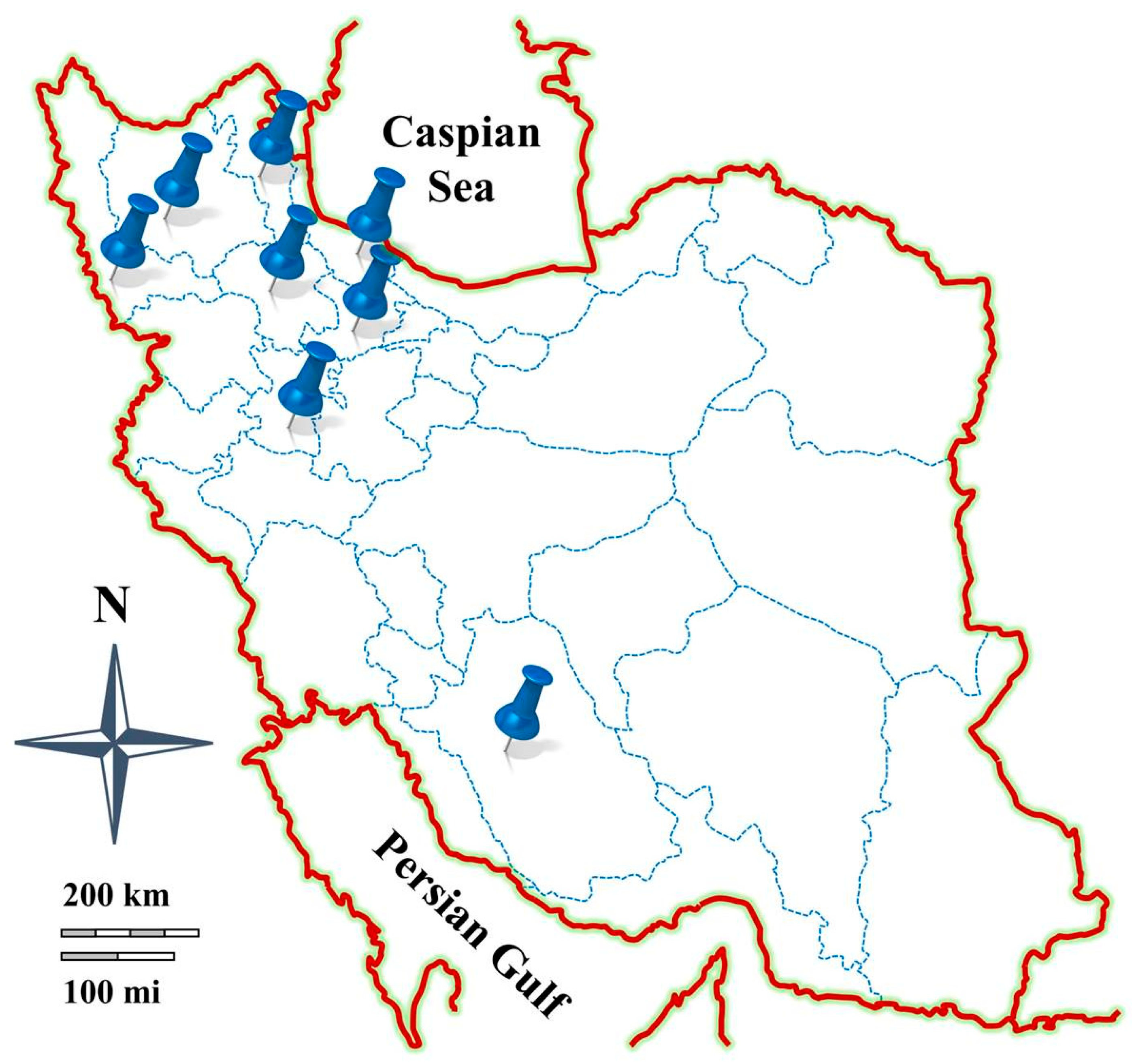
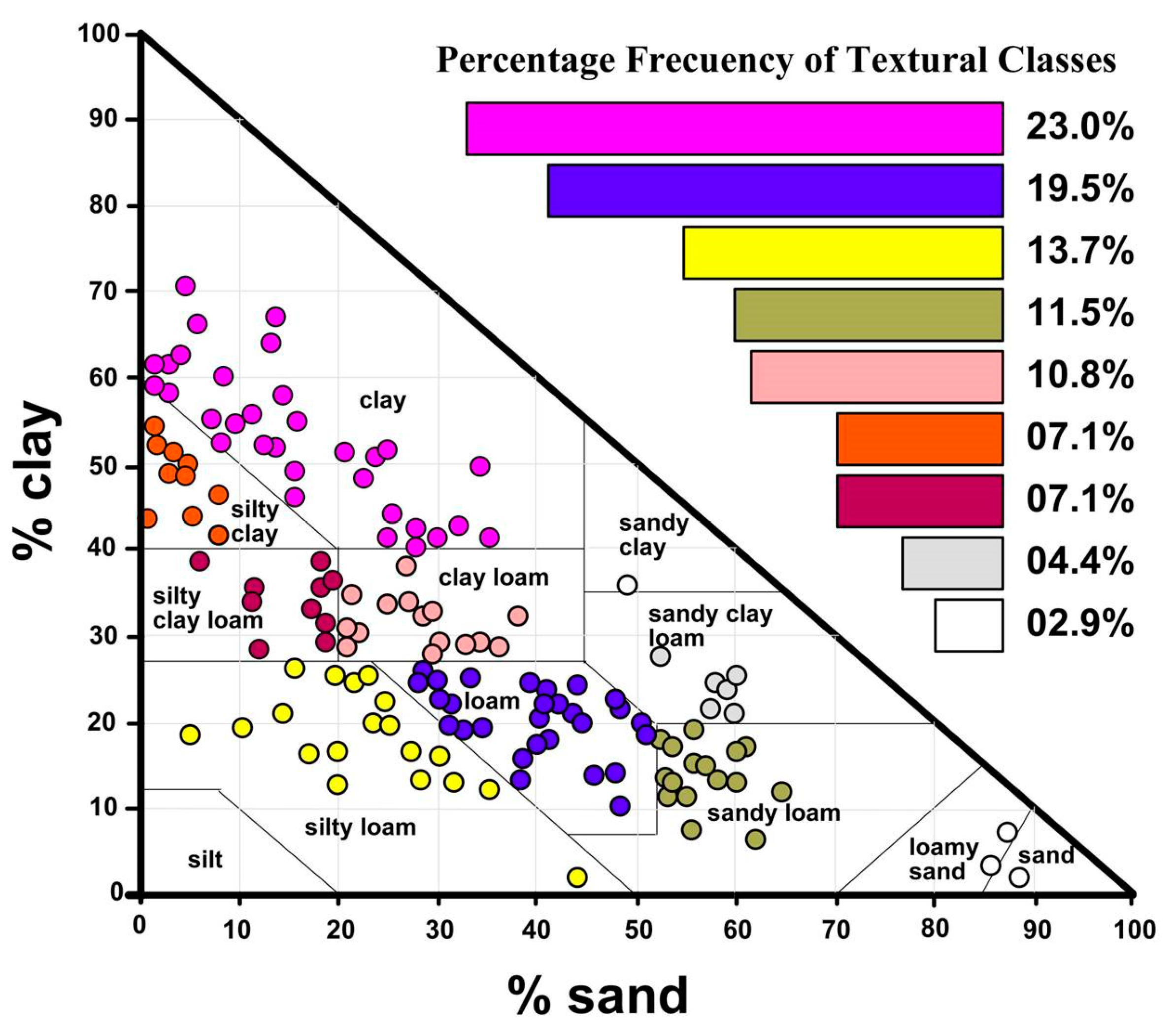
3.1. Soil Sampling and Characterization

Aiming to cover all textural classes, 140 samples were selected from different provinces of Iran. The geographical location of the selected provinces is shown in Figure 1. For soil sampling, disturbed and undisturbed samples were taken from 0–15 cm depth. Laboratory experiments include water retention measurements as well as soil texture, organic matter, bulk density, and particle density.

Soil bulk density was measured on undisturbed samples using 100 cm³ stainless steel cylinders (5 cm internal diameter and 5.1 cm height). Collected samples were oven-dried at 105 °C for 24 h prior to bulk density (ρ_b) determinations [84]. To measure other soil properties, the disturbed soil samples were air-dried and sieved (2 mm mesh). The particle size distribution (sand, silt, and clay percentages) was determined using the hydrometer method [85]. Soil particle density was measured using a glass pycnometer. The soil organic matter was determined by the wet oxidation method [86,87].

Table 2. Summary of soil properties for the selected 140 soils.

Soil Properties	Mean	Max	Min	Standard Deviation
Clay (%)	31.34	70.51	2.12	16.13
Silt (%)	38.05	69.97	4.78	12.81
Sand (%)	30.61	88.97	1.11	19.21
Bulk Density (g cm−3)	1.38	1.91	0.95	0.19
Particle Density (g cm−3)	2.54	2.71	2.23	0.10
Organic Matter (%)	1.51	4.63	0.21	0.77

summarizes soil properties for the 140 samples, and Figure 2 displays soil texture, including the frequency of each textural class. The international classification of the studied soils includes Saline Alluvial soils, Salt March soils, Lithosols, Brown soils, Calcareous lithosols, Brown soils and Chestnut soils, and Fine textured Alluvial soils. As shown in Table 2, bulk density ranges from 0.95 to 1.91 g cm⁻³, with particle density from 2.23 to 2.71 g cm⁻³. Organic matter is low, with values between 1.51 to 4.63%.

3.2. SWR Measurements

Experimental SWR data for disturbed and undisturbed soil samples were performed in the laboratory. Standard suction experiments were divided into two groups: undisturbed soils for suction measurements below 1 bar (1000 cm H₂O) and disturbed soils for suction between 1 to 15 bar (1000 to 15,000 cm H₂O). After saturating the samples from the bottom for 24 h, they were drained to the corresponding suction level using different methods. A hanging column apparatus was used for suctions of 10, 20, 30, 40, 50, 60, 70, 80, and 90 cm H₂O using undisturbed soils. The ceramic pressure plate extractors were utilized for suctions of 100, 300, 1000, 3000, 5000, and 15,000 cm H₂O. It is noticeable that for suctions of 100, 300, and 1000, undisturbed soil samples and for suctions of 3000, 5000, and 15,000 cm, H₂O-disturbed soil samples were used. The soil samples were placed on porous pressure plates (ceramic). The soil was placed directly on the porous plates without using cheesecloth to retain the soil in the samples. The soil samples placed on the pressure plates were wetted from below and allowed to saturate overnight. The desired suction was applied to the samples. After that, no water was removed from the sample, which means that the samples reached equilibrium by suction. Soil samples were then removed from the pressure plates and immediately covered with the sample holder cap to prevent evaporation. The samples were immediately transferred to an oven for determination of the soil water content (105 °C for 24 h) [88].

3.3. Evaluation and Ranking Criteria

Statistical measures such as the root mean square error (RMSE), Akaike information criterion (AIC), and Bayesian information criterion (BIC) were used to assess and compare the performance and goodness-of-fit of the selected SWR models. RMSE represents the overall differences between the measured (observed) SWR data and the predicted (estimated) values by the corresponding SWR model. These deviations are known as residuals, and for the complete fitted SWR curve, the residual sum of squares approaches zero [47]:

$$RMSE=\sqrt{\frac{1}{n}\sum _{i=1}^n{({\theta }_{i,Estimated}-{\theta }_{i,Observed})}^2}$$

(16)

where, ${\theta }_{i,Estimated}$ and ${\theta }_{i,Observed}$ refer to the estimated and measured soil water content, respectively, and n is the number of measured suction data points. The AIC test allows comparison and ranking of the models with disparate parameters (type and number):

$$\left\{\begin{array}{ll}N \mathrm{l}\mathrm{n} \left(\frac{RSS}{N}\right)+2K& \frac{N}{K}\ge 40\\ N \mathrm{l}\mathrm{n} \left(\frac{RSS}{N}\right)+2K+\frac{2K(K+1)}{N-K-1}& \frac{N}{K}<40\end{array}\right.$$

(17)

where K is the number of adjustable parameters in the model, N is the number of suction data points to be fitted, and RSS is the residual sum of squares. For two fitting models, the one with a lower AIC value is suggested better [89,90].

BIC is a model selection criterion, which is modified from the AIC criterion. The penalty term for BIC is similar to the AIC equation but uses a multiplier of ln(N) for K instead of a constant value of 2 by incorporating the sample size N. This allows to resolve the overfitting problem in data fitting [91]:

$$N \mathrm{l}\mathrm{n} \left(\frac{RSS}{N}\right)+K \mathrm{l}\mathrm{n} \left(N\right)$$

(18)

3.4. Analysis of 4 and 5 Parameter Logistic Curves

The general or standard form of four- and five-parameter logistic curves (4PLC and 5PLC) are represented by Equations (19) and (20) [92]:

$$\mathrm{y}=A_{min}+\frac{A_{max}-A_{min}}{\left[1+{\left(\frac{x}{c}\right)}^d\right]}$$

(19)

$$\mathrm{y}=A_{min}+\frac{A_{max}-A_{min}}{{\left[1+{\left(\frac{x}{c}\right)}^b\right]}^d}$$

(20)

where coefficients A_min and A_max indicate the minimum and maximum values of the dependent variable and somehow control the location of the upper and the lower asymptotes of the Equation. Coefficient c controls the location of the transition on the x-axis and refers to the inflection point in the transition between the two asymptotes. Coefficient b is the slope at the transition point c and controls the rate of approach to the asymptotes. The sign of b controls whether the curve is monotonically ascending or descending. Coefficient d controls the degree of asymmetry in an arbitrary 5PLC. This is the difference in the rates of approach from the inflection point c to the lower and the upper asymptotes. Indeed, the 5PLC model is the extended edition of the 4PLC with more flexibility to control the asymmetry of the curve [93]. The 4PLC is point symmetric on semi-log axes about its midpoint.

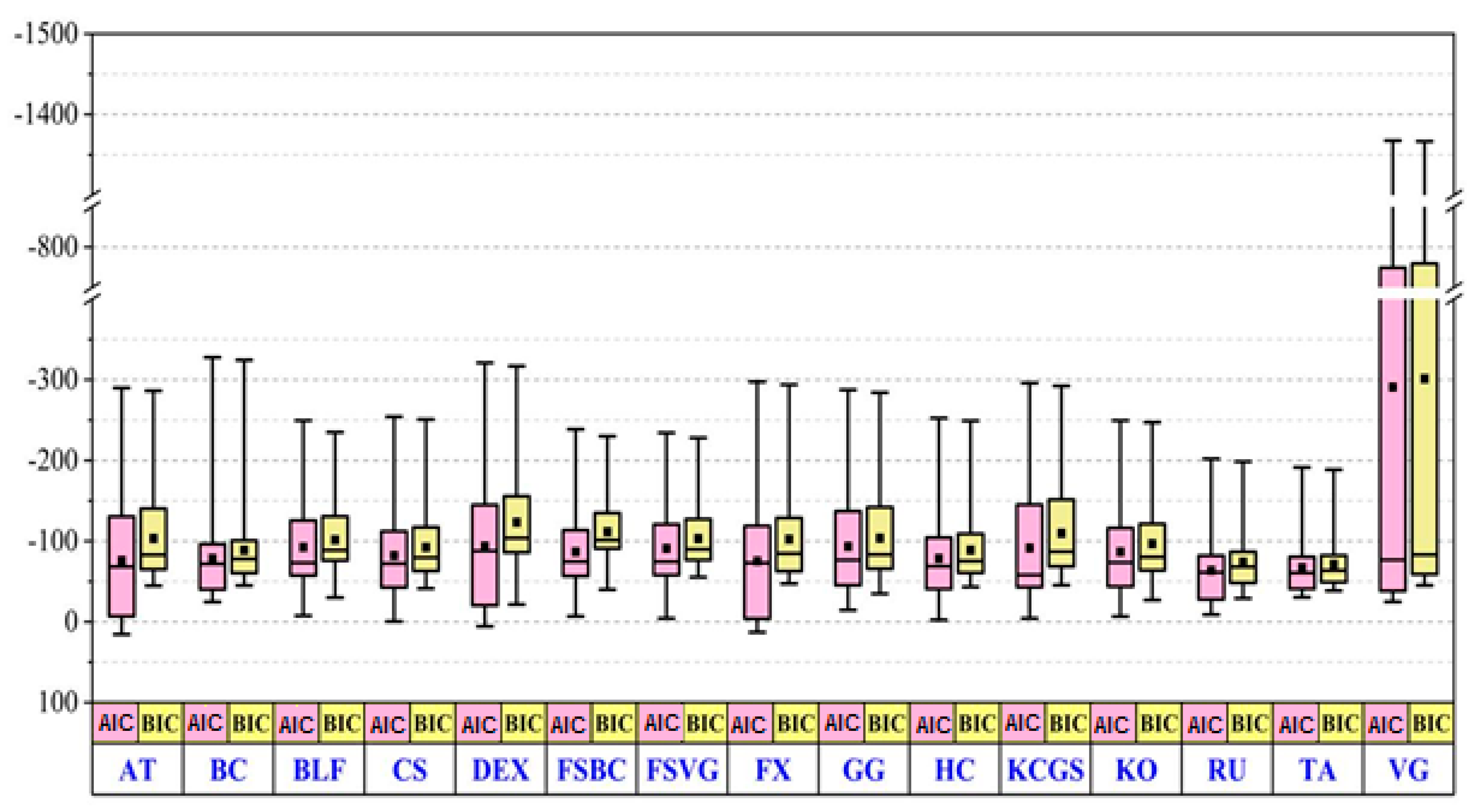
3.5. Effect of K on AIC and BIC

AIC and BIC facilitate and make it possible to compare models with a different number of parameters under equal conditions. As already mentioned, for different models, the one with the smaller AIC value is suggested to be a better model for the dataset. When comparing the fitting accuracy and performance of different models with different numbers of parameters and identical RSS, priority is given to the model with fewer parameters. Besides the smaller AIC (or BIC), a lower correlation between parameters results in increased uniqueness for estimated values. For example, considering two models with K and K + 1 parameters, substituting K + 1 in Equation (17) results in the following:

$$\begin{array}{c}{AIC}_{K+1}=N \mathrm{l}\mathrm{n}\left(\frac{RSS}{N}\right)+2\left(K+1\right)+\frac{2\left(K+1\right)\left(K+1+1\right)}{N-\left(K+1\right)-1}\\ \approx {AIC}_K+\frac{2(N+K)}{N-K-2}\end{array}$$

(21)

The above Equation indicates that regardless of the number of fitting data points (N), the addition of one additional fitting parameter to the model increases AIC linearly.

4. Results and Discussions

Figure 3 and Figure 4 and

Table 3. Statistical details from box-and-whisker plots for RMSE, AIC, and BIC (15 SWRC models are fitted to 140 empirical retention datasets). Model abbreviations: BC: Brooks and Corey model, VG: van Genuchten model, TA: Tani model, RU: Russo model, CS: Campbell and Shiozawa model, FX: Fredlund and Xing model, HC: Hutson and Cass model, KO: Kosugi model, GG: Groenevelt and Grant model, DEX: Dexter et al. double exponential model, ATB: Assouline, Tessier, and Beruand model, BLF: Romano et al. Bimodal Lognormal Function, KCGS: Khlosi et al. model, FSBC: modified BC model by Fayer and Simmons. FSVG: modified VG model by Fayer and Simmons.

	RMSE			AIC			BIC
Model	10%	50%	90%	10%	50%	90%	10%	50%	90%
BC	0.0059	0.0150	0.0300	−119.3	−71.8	−30.7	−119.8	−77.8	−51.0
VG	0.0001	0.0115	0.0274	−783.7	−78.7	−30.5	−778.8	−83.1	−50.9
TA	0.0168	0.0308	0.0447	−107.2	−60.8	−23.7	−106.9	−63.7	−44.7
RU	0.0129	0.0264	0.0434	−106.4	−61.3	−16.1	−106.7	−62.6	−44.2
CS	0.0035	0.0118	0.0241	−128.2	−72.0	−34.4	−128.8	−79.6	−54.5
FX	0.0014	0.0093	0.0233	−149.7	−72.9	−16.8	−151.1	−84.6	−53.4
HC	0.0043	0.0147	0.0275	−119.1	−68.7	−34.1	−123.6	−75.3	−54.3
KO	0.0020	0.0097	0.0250	−143.8	−73.4	−35.3	−146.6	−80.2	−54.8
GG	0.0009	0.0096	0.0219	−149.3	−76.6	−34.8	−153.1	−83.3	−55.2
DEX	0.0016	0.0074	0.0196	−154.7	−72.4	−38.7	−157.7	−85.3	−61.3
ATB	0.0009	0.0096	0.0201	−140.9	−68.3	−12.9	−150.5	−82.9	−56.9
BLF	0.0039	0.0095	0.0247	−135.3	−73.2	−48.7	−151.2	−81.8	−55.0
KCGS	0.0017	0.0082	0.0236	−161.2	−58.1	−34.7	−171.2	−87.0	−59.4
FSBC	0.0063	0.0126	0.0266	−129.7	−74.8	−49.8	−136.0	−83.2	−55.7
FSVG	0.0088	0.0113	0.0236	−145.4	−74.5	−47.9	−162.5	−83.2	−54.5

and

Table 4. Statistical detail of box-and-whisker plots for RMSE of the 15 fitted SWR curve models. Model abbreviations: BC: Brooks and Corey model, VG: van Genuchten model, TA: Tani model, RU: Russo model, CS: Campbell and Shiozawa model, FX: Fredlund and Xing model, HC: Hutson and Cass model, KO: Kosugi model, GG: Groenevelt and Grant model, DEX: Dexter et al. double exponential model, ATB: Assouline, Tessier, and Beruand model, BLF: Romano et al. Bimodal Lognormal Function, KCGS: Khlosi et al. model, FSBC: modified BC model by Fayer and Simmons. FSVG: modified VG model by Fayer and Simmons.

Model	50%	25%	75%	Max	Min	75–25%	Max–Min
BC	0.0150	0.0085	0.0207	0.1749	2.3 × 10−5	0.0122	0.1749
VG	0.0115	0.0001	0.0199	0.2274	9.5 × 10−17	0.0199	0.2274
TA	0.0308	0.0234	0.0365	0.0618	7.4 × 10−3	0.0132	0.0544
RU	0.0264	0.0188	0.0347	0.0954	2.8 × 10−3	0.0159	0.0926
CS	0.0118	0.0052	0.0179	0.0334	1.8 × 10−3	0.0127	0.0316
FX	0.0093	0.0025	0.0179	0.0376	1.1 × 10−4	0.0153	0.0375
HC	0.0147	0.0070	0.0194	0.0388	1.7 × 10−3	0.0124	0.0372
KO	0.0097	0.0041	0.0172	0.0377	1.9 × 10−4	0.0131	0.0375
GG	0.0096	0.0024	0.0163	0.0405	8.2 × 10−6	0.0139	0.0405
DEX	0.0074	0.0031	0.0130	0.0444	6.9 × 10−5	0.0099	0.0443
ATB	0.0096	0.0025	0.0152	0.0372	5.9 × 10−4	0.0127	0.0366
BLF	0.0095	0.0024	0.0161	0.0401	8.2 × 10−6	0.0137	0.0401
KCGS	0.0082	0.0012	0.0132	0.0390	1.8 × 10−6	0.0120	0.0390
FSBC	0.0126	0.0046	0.0151	0.0369	7.6 × 10−4	0.0105	0.0361
FSVG	0.0113	0.0028	0.0168	0.0377	3.1 × 10−5	0.0139	0.0376

show results corresponding to RMSE, AIC, and BIC of each SWR model using the 140 soils. According to Table 3, except for the Tani and Russo models, the 10% percentile of the other 13 models is <0.01, while the 50% percentile (median) of the other 13 models is <0.015. Therefore, selected SWR models have good performance in fitting SWR data.

Although for the Tani and Russo models the number of parameters is less than for other models, the shape of suggested functions does not correspond to the behavior of the SWR curve. Figure 5 clearly shows this demerit. Reducing the number of parameters in the model reduces the correlation between the parameters and increases the uniqueness of the parameters. The ideal SWR model will be able to account for the variations in the SWR data with the minimum number of parameters. Therefore, it is recommended to use models with fewer parameters in the fitting process as much as possible. The Tani and Russo models show the worst performance among the 15 utilized models; therefore, they are less recommended. According to Table 4, among the remaining 13 models, the maximum RMSE varies between 0.03 and 0.23, indicating that there are significant differences in the accuracy and performance of the models.

Figure 3 shows that for the BC and VG models, despite the acceptable median and 90% percentile for both models, drastic and unusual changes are observed for the RMSE (see Table 4), ranging from 2.3 × 10⁻⁵ to 0.175 and 9.5 × 10⁻¹⁷ to 0.227, respectively, indicating that these models are significantly sensitive to soil type (or soil textures) compared to other models. Based on the information in Table 3, the AIC and BIC analysis of the models also shows that the VG model has the lowest AIC and BIC among the selected models, so there are striking differences in the calculated AIC and BIC for the 10% percentile resulting from the minimum 10% percentile for the RMSE. It seems that for some soils the VG model has an excellent fit compared to other models. The reason for this peculiarity is discussed in the manuscript. From Equation (17), by increasing the performance and accuracy of the desired model in fitting the experimental data (goodness-of-fit) and also the number of empirical SWR data (N), $\frac{RSS}{N}$ approaches zero (0⁺ or zero limit). As a result, $\mathrm{l}\mathrm{n}\left(\frac{RSS}{N}\right)$ takes more negative values. In Table 3, models with more negative AIC (in other words, lower values) have higher accuracy.

The AIC and BIC results for the 15 selected models are shown in Figure 4. The results show that despite the relative proximity for the 50% percentile (median) in all models, the VG model results in wide alterations for AIC and BIC. It appears that the performance of the model is influenced by soil type and soil physical properties.

BC and VG reformulated and transformed Equations (19) and (20) to Equations (1) and (2), where the minimum and maximum soil water contents, θ_r and θ_s, are replaced by A_min and A_max, respectively. Although these models, like the traditional models, have acceptable performance for different soil types, they have some fundamental weaknesses and drawbacks, as discussed below.

(1)

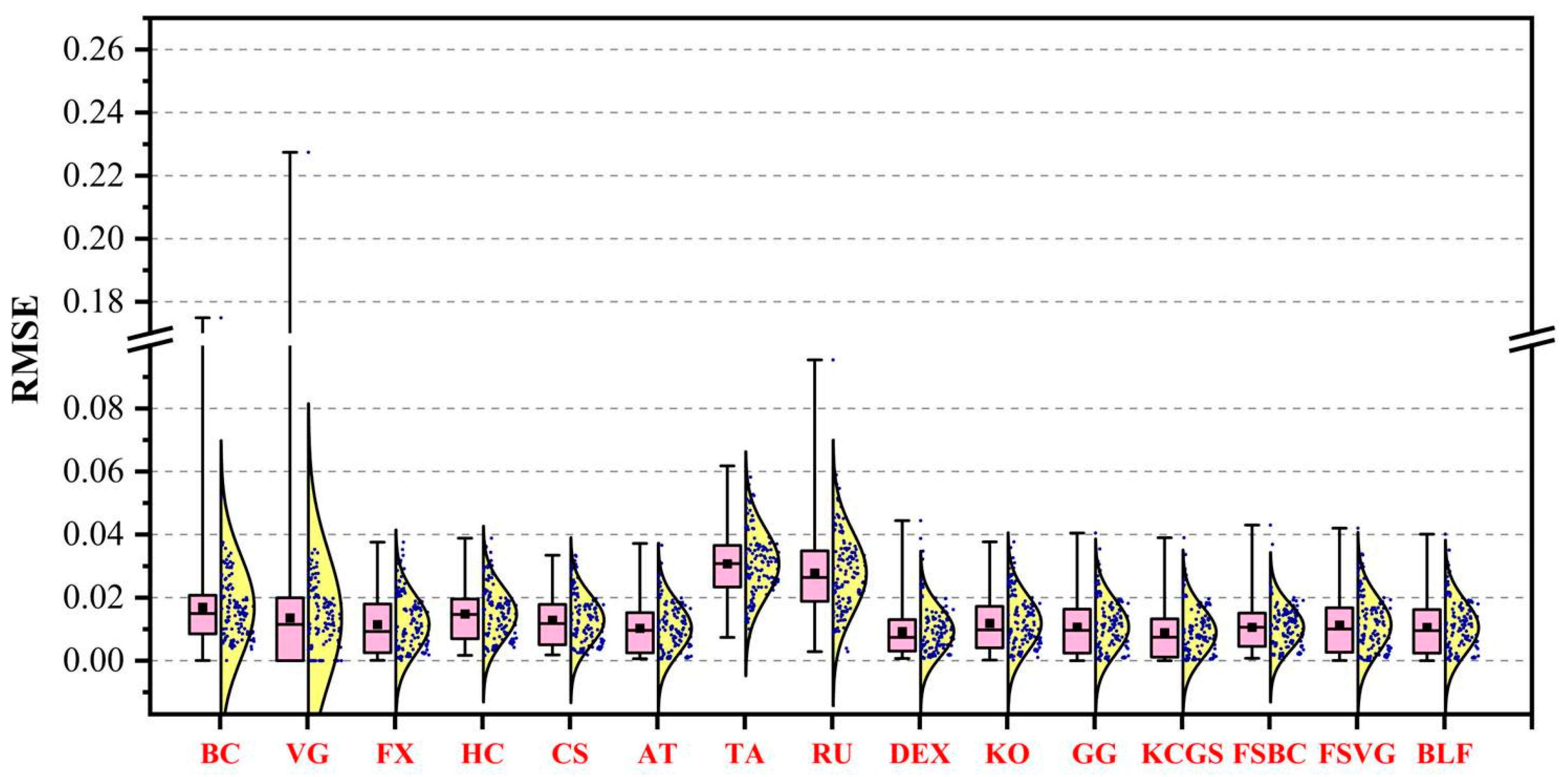
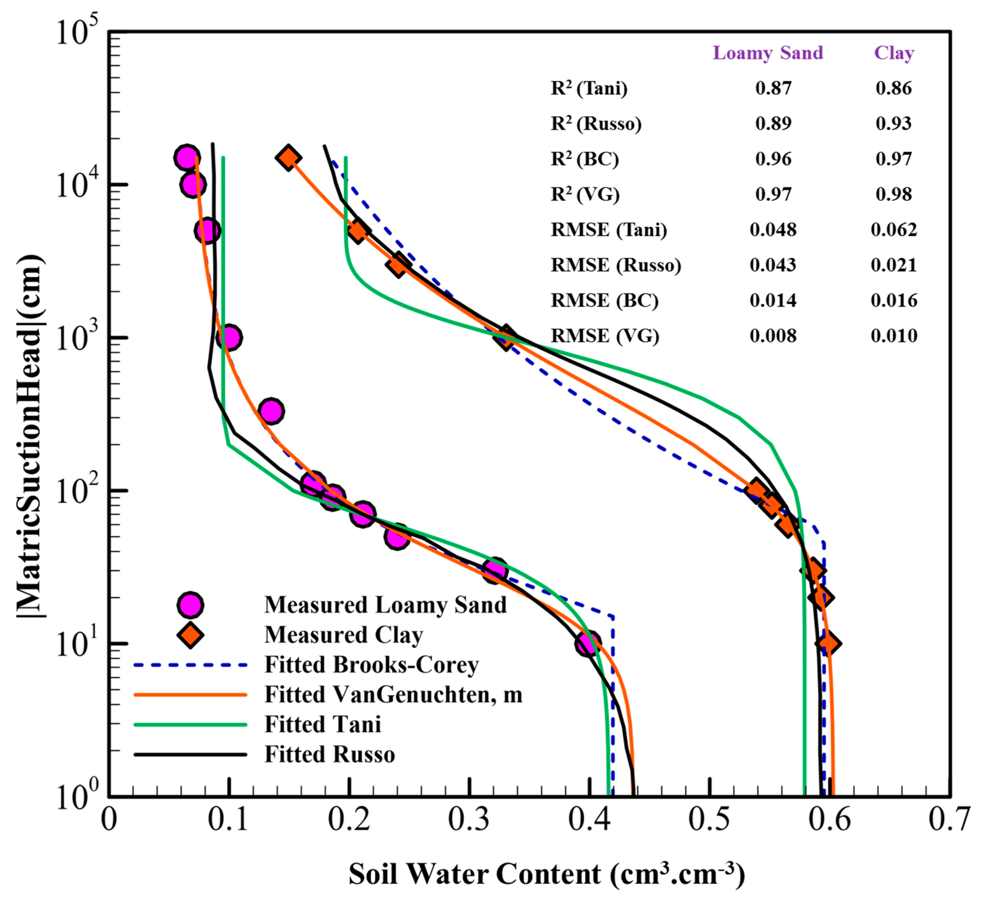
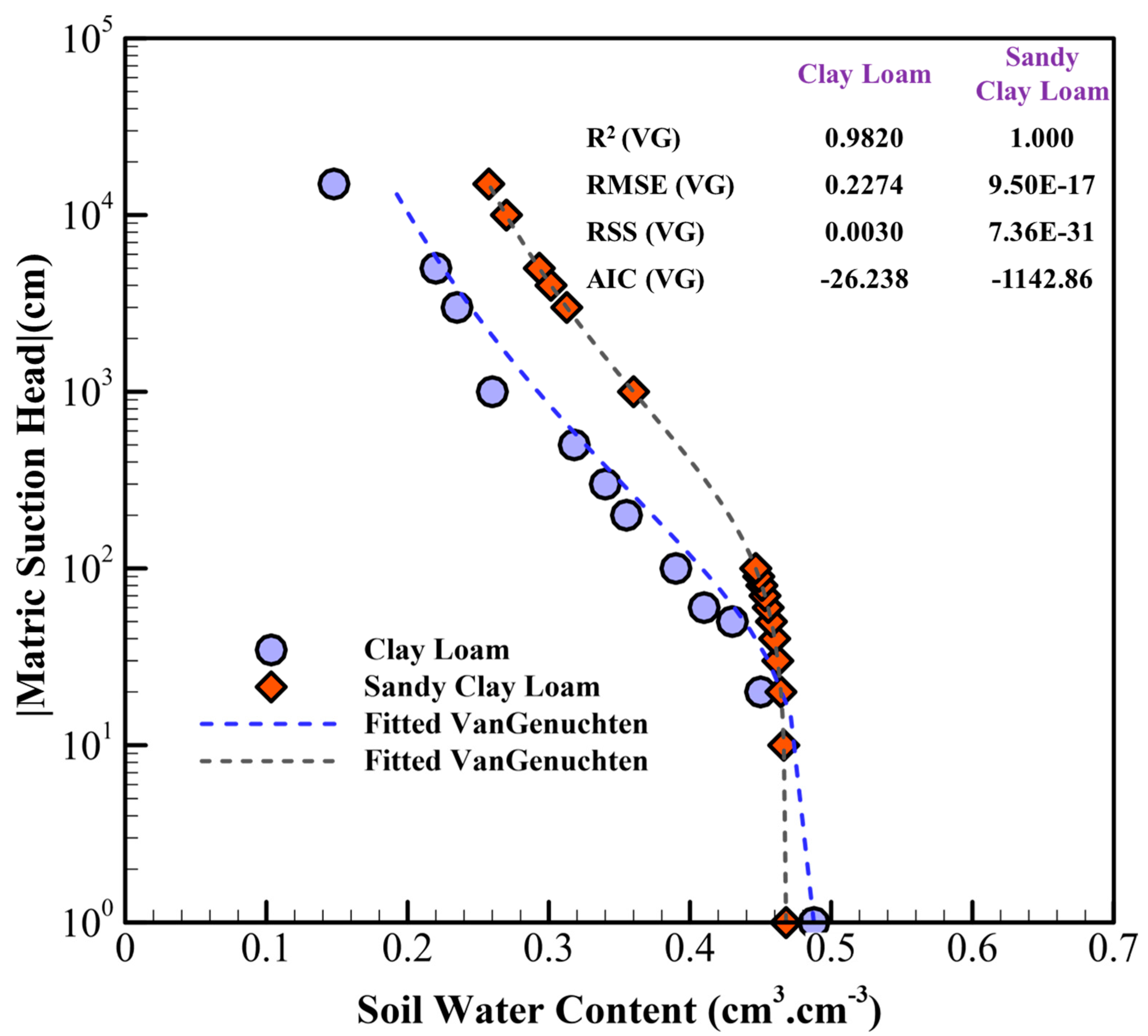
Given the nature and behavior of Equations (19) and (20), BC and VG models show excellent fit to the asymmetric retention data around the inflection point with RMSE < 10⁻¹⁰ but are inherently and significantly sensitive to pure errors and outliers in the dataset. Pure errors are errors caused by the presence of random variation in the data such that despite high R² values, the RMSE shows abnormal values (see Figure 6, Figure 7 and Figure 8).

The residual sum of squares can be decomposed into two components:

RSS = (sum of squares due to “pure error”) + (sum of squares due to “lack of fit”)

The sum of squares due to “pure error” is the sum of squares of the differences between each observed y-value (water content) and the average of all y-values ($\overline{\theta }$) corresponding to the same x-value (matric suction). The sum of squares due to lack of fit is the weighted sum of squares of differences between each average of y-values ($\overline{\theta }$) corresponding to the same x-value and the corresponding fitted y-value (θ_Estimated), the weight in each case being simply the number of observed y-values for that x-value:

$$\begin{array}{ll}RSS=& {\displaystyle \sum _{i=1}^N}{\left(measured value-fitted value\right)}^2=\\ & \underset{pure error}{\underbrace{{\displaystyle \sum _{i=1}^N}{\left(measured value-local average\right)}^2}}\\ & +\underset{lack of fit}{\underbrace{{\displaystyle \sum _{i=1}^N}{weight\times \left(local average-fitted value\right)}^2}}\end{array}$$

(22)

To minimize pure errors and obtain accurate empirical SWR for each soil sample, replication and duplication simultaneously are used during experiments so that no outliers were observed for almost 99% of the averaged SWR data. To avoid abnormal and illusive RMSEs, a few scattered outliers were ignored. In the presence of pure errors and the erratic scattering of data around the regression curve, suitable R² values are obtained (see Figure 6, Figure 7 and Figure 8 as typical examples), which by itself is not an acceptable criterion for measuring the accuracy of the model (Figure 5). The best criteria to assess models’ performance are RSS, RMSE, and AIC;

(2)

Comparison of Equations (1) and (19) and Equations (2) and (20) shows that for the BC and VG models, θ_r and θ_s are considered as the corresponding soil water content values when the logarithm of the matric suction approaches zero and infinity, respectively. Therefore, these parameters are fitting parameters without any specific physical meaning. From the data fitting, the range of variation for θ_r was higher compared to other models (0.00001 to 0.24 m³·m⁻³), indicating that these models, regardless of soil type and data range, only tried to fit the data with unphysical θ_r;

(3)

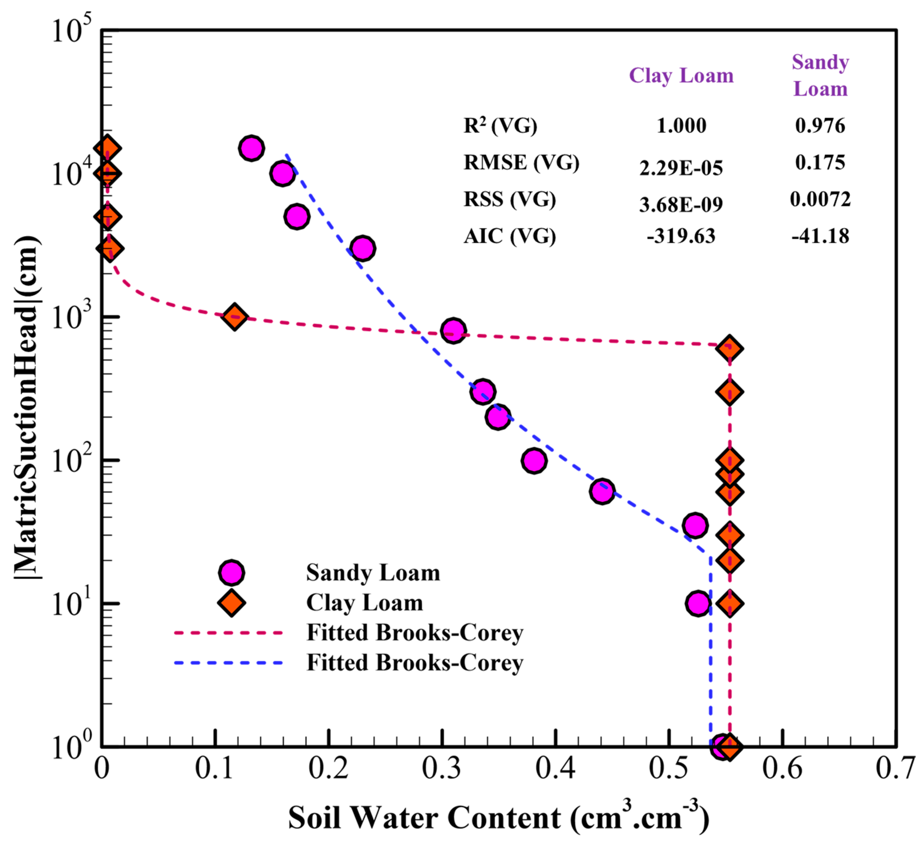
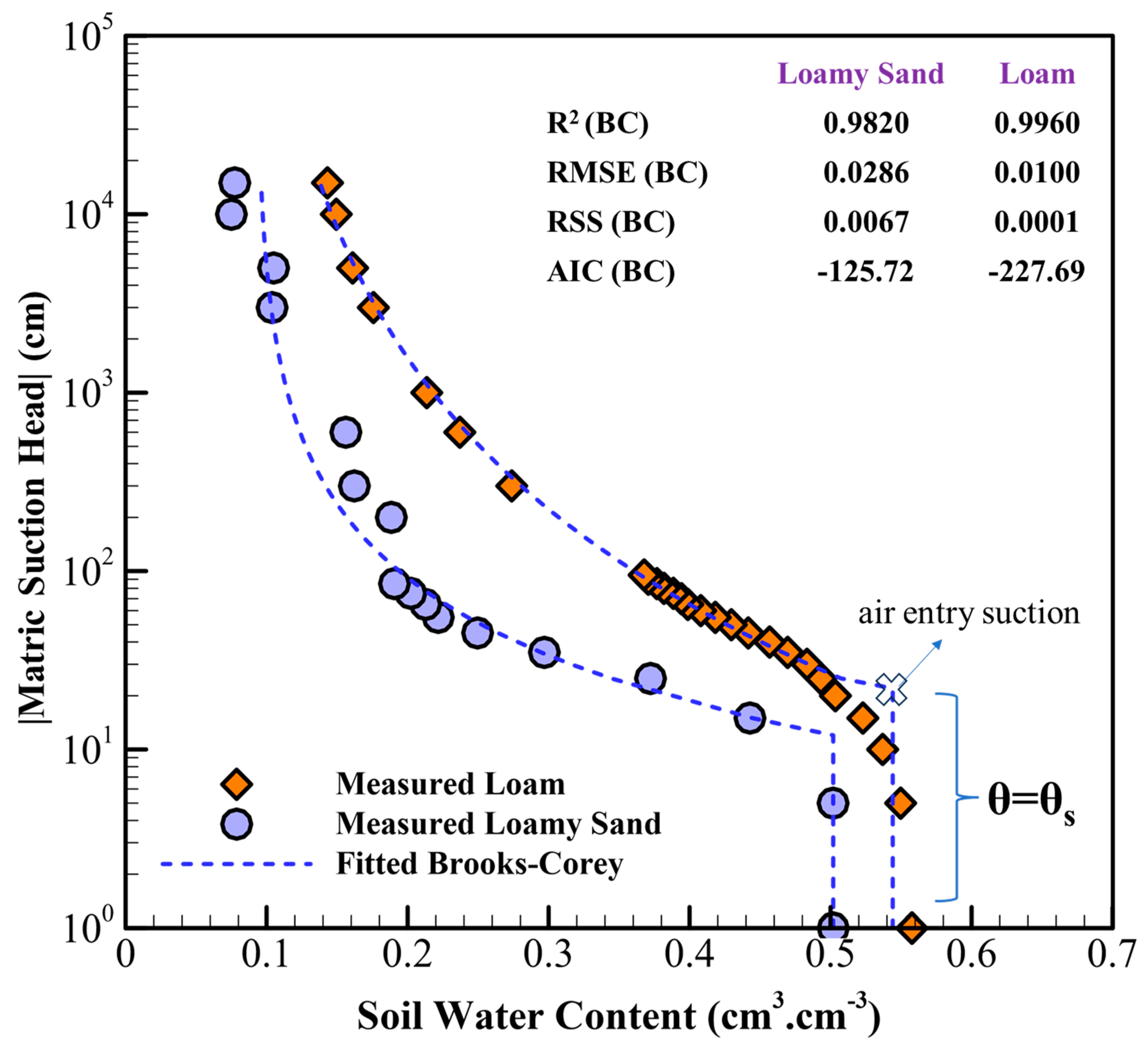
For matric suction below air entry, the BC model treats the SWR curve as a vertical line (Figure 6, Figure 7 and Figure 8). In other words, as depicted in Figure 8 for suctions below air entry, decreasing suction does not increase soil water content and its value remains constant to saturated water content. For fine textured soils with large h_a, the inability of the model to simulate this part of the SWR becomes more pronounced, resulting in an increase in the RMSE;

(4)

The VG model does not consider the matric suction at the air entry suction. However, the strength of the model lies in having an inflection point which results in an exceptional fit to measured data, particularly at high water content;

(5)

As previously discussed, the BC and VG models assume that soil suction approaches zero and infinity as the water content decreases to θ_r and increases to θ_s, respectively. This results in the constant maintenance of θ_r with additional matric suction. While this may be valid only for the wet part of the SWR, however, a large number of observed SWR data indicates that for the dry part of the SWR (θ < θ_r), increasing matric suction results in a decrease in water content that follows a linear relationship on a semi-logarithmic scale [38,94]. Given the domain and range of 4- and 5PLCs, the major drawback of the BC and VG models is that they do not define the SWR beyond θ_r;

(6)

The correlation between parameters plays a significant role in the sensitivity of the SWR model to the experimental data. In the VG model, the relationship between the three parameters of α, n, and m is such an extent that minor alteration in one parameter effectively changes the other two parameters. To better understand the sensitivity of the VG model, the correlation matrix between the VG model parameters (θ_r, θ_s, α, n, and m) for the maximum and minimum RMSE, RSS, and AIC (see Figure 6, which shows the worst and the best fits corresponding to clay loam and sandy clay loam soils) are presented in

Table 5. Calculated binary correlation matrix between VG model parameters (θ_r, θ_s, α, n, and m) corresponding to Figure 6 (worst and best performance of the VG model). (a) Relates to the sandy clay loam and (b) notes to the clay loam.

(a)	θᵣ	θs	α	n	m
θᵣ	1
θs	0.341	1
α	−0.948	−0.380	1
n	−0.827	−0.657	0.968	1
m	0.977	0.452	−0.985	−0.924	1
(b)	θᵣ	θs	α	n	m
θᵣ	1
θs	0.002	1
α	−0.967	0.037	1
n	−0.805	−0.009	0.933	1
m	0.924	0.008	−0.980	−0.996	1

.

The binary correlation matrix clearly shows that, regardless of model performance and good-of-fitness, there is a high dependency between the three parameters (α, n, and m) of the VG model.

The impact of soil properties on the performance of the SWR models is evaluated for the 140 soils. The RMSE of each SWR model was correlated with the sand-silt-clay content, bulk density, and organic matter. Results are summarized in

Table 6. Pearson correlation coefficient (PCC, p-value) between RMSE and soil sand-silt-clay content, bulk density (ρ_b), and organic matter (OM) plus related p-values at the significance level of 0.05. SWR model abbreviations are indicated in Table 1.

Model	Sand	p-value	Clay	p-value	Silt	p-value	ρb	p-value	OM	p-value
BC	0.07	0.40	−0.11	0.21	0.02	0.81	0.02	0.84	−0.14	0.08
VG	0.02	0.80	−0.06	0.48	0.04	0.61	−0.04	0.63	−0.01	0.06
TA	−0.17	0.05	−0.01	0.96	0.25	0.01	−0.09	0.31	−0.13	0.12
RU	−0.01	0.92	−0.11	0.20	0.15	0.08	−0.03	0.71	−0.09	0.11
CS	−0.06	0.46	−0.09	0.29	0.20	0.02	−0.19	0.04	−0.05	0.08
FX	0.03	0.71	−0.18	0.02	0.19	0.03	−0.03	0.11	−0.23	0.01
HC	0.07	0.38	−0.13	0.11	0.05	0.49	−0.16	0.06	0.09	0.11
KO	0.03	0.66	−0.15	0.07	0.13	0.11	−0.09	0.06	−0.17	0.08
GG	−0.01	0.95	−0.15	0.06	0.20	0.01	−0.10	0.07	−0.15	0.06
DEX	0.13	0.01	−0.22	0.01	0.08	0.36	−0.13	0.05	−0.04	0.06
ATB	0.17	0.03	−0.21	0.02	0.01	0.97	−0.12	0.10	−0.09	0.09
BLF	0.08	0.29	−0.20	0.01	0.12	0.18	0.17	0.04	−0.10	0.08
KCGS	−0.04	0.58	−0.10	0.27	0.19	0.02	−0.07	0.09	−0.18	0.06
FSBC	0.07	0.37	−0.16	0.05	0.09	0.27	−0.16	0.06	−0.07	0.12
FSVG	−0.06	0.47	−0.08	0.29	0.20	0.01	−0.09	0.08	0.05	0.09

.

In the current study, the null hypothesis (H₀) is considered when there is no correlation between RMSE (model performance) and soil properties (sand-silt-clay content, bulk density, and organic matter) in the overall population, including 140 soil samples ($r\approx 0$). On the counterpoint, for the alternative hypothesis (H₁), there is a correlation between RMSE and soil properties in the overall population ($r\ne 0$). To accept H₁, calculated p-values must be less than 0.05 or 0.01 for 95% and 99% confidence intervals, respectively. To conclusively convict and reject H₀, p-values must be less than 10⁻³.

Regarding the corresponding p-values in Table 6, it can be inferred that for the BC and VG models, there is a weak correlation between model performance (RMSE) and soil properties (sand-silt-clay content, bulk density, and organic matter) in the overall population including 140 soil samples. As mentioned before, the VG model is a closed-form sigmoid expression including the adjustable parameters obtained from fitting. In the VG model, m and n are called shape (fitting) parameters and do not have a physical meaning.

From Table 6, it can be concluded that for the BC and VG models, the model performance is strongly independent of soil texture and bulk density. On the other hand, almost in all SWR models, the model performance is impacted by organic matter, with 90% confidence. However, the calculated correlation between organic matter and RMSE is not striking, and correlations are negligible.

Another important finding from Table 6 is the Dexter (double exponential) model, where the model performance is noticeable under the influence of soil properties.

Evaluation of Equation (14) can shed more light on Table 6 results. DEX developed model has five adjustable parameters with physical meaning. The parameters of this model correspond to the soil matrix and the structural pore space. In general, for this model, the pore configuration in the soil specifies the shape of the function. In Equation (14), w is the gravimetric soil water content associated with the matric suction, C points to the asymptote of the model when it approaches the residual soil water content, A₁ and A₂ are parameters of the model associated with the matrix and structural pores of the soil, respectively, and h₁ and h₂ are related to the matric suction when water drains from the textural (matrix) and the structural pore space, respectively.

It can be deduced that the Dexter model is bimodal. The first part, (A₁ exp(h/h₁)), represents the matrix pores, and the second part, (A₂ exp(h/h₂)), considers the effect of structural pores on the SWR curve.

Table 6 also shows that at the significance level of 0.05, the PCC between RMSE and soil texture shows higher values compared to ρ_b and OM. The findings of Table 6 are consistent with Cornelis et al. [95] and Du [22]. When correlating the RMSE of the SWR model with OM and ρ_b, Cornelis et al. [95] found no significant results at the 0.05 level. They compared 48 soil samples from Belgium using unimodal analytical expressions, evaluating the accuracy, linearity, AIC, and prediction potential (PCC). Du [22] studied the performance of closed-form expressions on 94 soil samples from saturation to oven-dry. Cornelis et al. [95] observed that the VG model with m as a free parameter showed the highest accuracy and the lowest AIC. However, it had a low prediction potential, which means that the model is remarkably influenced by soil texture. Constraining m to 1 − 1/n did not resolve this issue. However, reducing the number of parameters from 5 to 4 mitigated the model’s dependence on soil texture. Both studies, Cornelis et al. [95] and Du [22] found a slight correlation between RMSE and ρ_b, as well as RMSE and OM, for most SWR models, which is attributed to the specific mathematical form of these models. The parameters within the models are primarily defined through the integration of features such as PSD and capillarity laws.

The SWR models show weak dependence on ρ_b and OM due to the narrow range of variation in these parameters. However, when compared to previously published data [38,95,96,97] and UNSODA data [98], some variations can be observed.

Evaluation of PCC between RMSE and the soil sand-silt-clay content reveals some interesting features. For all SWR models, the RMSE values are negatively correlated with clay. On the other hand, RMSE values are positively correlated with silt, indicating that by increasing clay content and decreasing silt content, the performance of the SWR model increases (this effect is weak). For sand, RMSE and SWR models exhibit contrasting patterns. The performance of all SWR models in Cornelis et al. [95] except one is also in agreement with these results.

5. Conclusions

In this study, the performance and predictive potential of 15 soil water retention (SWR) models have been assessed using 140 soils from Iran. The findings indicate important conclusions summarized below.

Based on the Akaike information criterion (AIC) and Bayesian information criterion (BIC), the van Genuchten model has the lowest values. There are significant differences in AIC and BIC for the 10% percentile, which are a result of the minimum RMSE at the 10% percentile. This can be attributed to the symmetric SWR data around the inflection point, where the minimum RMSE values for these soils were 10⁻¹⁷. The Brooks and Corey and van Genuchten models demonstrate inadequate predictive ability in estimating SWR curves. Results from the statistical test conducted at a significance level of 0.05 (95% confidence) demonstrate that soil texture has not notable impact on both models, as suggested by calculated p-values for PCC between RMSE and soil texture. Despite the relative proximity for the 50% percentile (median) in all models, the van Genuchten model results in wide alterations for AIC and BIC. It reveals that the performance of the model is influenced by soil type and soil physical properties.

The calculated Pearson correlation coefficient and associated p-values between RMSE and organic matter reveal that in almost all SWR models, the model performance is weakly influenced by organic matter, with an acceptable approximation (90% confidence). This independence is also evident for the bulk density, apart from in four models BC, VG, Tani, and Russo. Statistical investigation also reveals that the performance of the Dexter model is noticeably influenced by soil properties. The parameters of the Dexter model correspond to the soil matrix and the structural pore space, which is directly related to the shape of the SWR function.

The TA and RU models exhibit the poorest performance and accuracy compared to the studied SWR models. Among the SWR models, Dexter et al. double exponential, Groenevelt and Grant, and Khlosi et al. models show higher accuracy and performance in predicting the SWR curve in terms of RMSE, AIC, and BIC. The evaluation of prediction potential for SWR models reveals that the DEX, GG, Kosugi, Assouline, Tessier, and Beruand models show the least dependency on soil properties.

It should be noted that a small number of sandy soils were used in the data set, and therefore, the results may not be fully generalizable to sandy soils.

References

- Leij, F.J.; Russell, W.B.; Lesch, S.M. Closed-form expressions for water retention and conductivity data. Groundwater 1997, 35, 848–858. [Google Scholar] [CrossRef]
- Rasoulzadeh, A.; Sepaskhah, A.R. Advanced Topics in Soil Water Physics, Volume 1: Soil Water Characteristic Curve; University of Mohaghegh Ardabili Press: Ardabil, Iran, 2022; p. 304. (In Persian) [Google Scholar]
- Rasoulzadeh, A.; Sepaskhah, A.R.; Asghari, A.; Ghavidel, A. Long-term effects of barley residue managements on soil hydrophysical properties in north-western Iran. Geoderma Reg. 2022, 30, e00552. [Google Scholar] [CrossRef]
- Dobriyal, P.; Qureshi, A.; Badola, R.; Hussain, S.A. A review of the methods available for estimating soil moisture and its implications for water resource management. J. Hydrol. 2012, 458–459, 110–117. [Google Scholar] [CrossRef]
- Rashid, N.S.A.; Askari, M.; Tanaka, T.; Simunek, J.; van Genuchten, M.T. Inverse estimation of soil hydraulic properties under oil palm trees. Geoderma 2015, 241–242, 306–312. [Google Scholar] [CrossRef]
- Verbist, K.; Cornelis, W.M.; Gabriels, D.; Alaerts, K.; Soto, G. Using an inverse modelling approach to evaluate the water retention in a simple water harvesting technique. Hydrol. Earth Syst. Sci. 2009, 13, 1979–1992. [Google Scholar] [CrossRef]
- Zakizadeh Abkenar, F.; Rasoulzadeh, A. Functional Evaluation of Pedotransfer Functions for Simulation Of Soil Profile Drainage. Irrig. Drain. 2019, 68, 573–587. [Google Scholar] [CrossRef]
- Le Bourgeois, O.; Bouvier, C.; Brunet, P.; Ayral, P.A. Inverse modeling of soil water content to estimate the hydraulic properties of a shallow soil and the associated weathered bedrock. J. Hydrol. 2016, 541, 116–126. [Google Scholar] [CrossRef]
- Brooks, R.H.; Corey, A.T. Hydraulic Properties of Porous Media, 3rd ed.; Colorado State University: Fort Collins, CO, USA, 1964. [Google Scholar]
- van Genuchten, M.T. A Closed-form Equation for Predicting the Hydraulic Conductivity of Unsaturated Soils. Soil Sci. Soc. Am. J. 1980, 44, 892–898. [Google Scholar] [CrossRef]
- Arya, L.M.; Paris, J.F. A Physicoempirical Model to Predict the Soil Moisture Characteristic from Particle-Size Distribution and Bulk Density Data. Soil Sci. Soc. Am. J. 1981, 45, 1023–1030. [Google Scholar] [CrossRef]
- Kosugi, K. Lognormal distribution model for unsaturated soil hydraulic properties. Water Resour. Res. 1996, 32, 2697–2703. [Google Scholar] [CrossRef]
- Dexter, A.R.; Czyz, E.A.; Richard, G.; Reszkowska, A. A user-friendly water retention function that takes account of the textural and structural pore spaces in soil. Geoderma 2008, 143, 243–253. [Google Scholar] [CrossRef]
- Pollacco, J.A.P.; Fernández-Gálvez, J.; Carrick, S. Improved prediction of water retention curves for fine texture soils using an intergranular mixing particle size distribution model. J. Hydrol. 2020, 584, 124597. [Google Scholar] [CrossRef]
- Cueff, S.; Coquet, Y.; Aubertot, J.N.; Bel, L.; Pot, V.; Alletto, L. Estimation of soil water retention in conservation agriculture using published and new pedotransfer functions. Soil Tillage Res. 2021, 209, 104967. [Google Scholar] [CrossRef]
- Rasoulzadeh, A. Estimating Hydraulic Conductivity Using Pedotransfer Functions. In Hydraulic Conductivity: Issues, Determination and Applications; BoD–Books on Demand: Norderstedt, Germany, 2011. [Google Scholar] [CrossRef]
- van den Berg, M.; Klamt, E.; van Reeuwijk, L.P.; Sombroek, W.G. Pedotransfer functions for the estimation of moisture retention characteristics of Ferralsols and related soils. Geoderma 1997, 78, 161–180. [Google Scholar] [CrossRef]
- Huang, G.H.; Zhang, R.D.; Huang, Q.Z. Modeling Soil Water Retention Curve with a Fractal Method. Pedosphere 2006, 16, 137–146. [Google Scholar] [CrossRef]
- Tyler, S.W.; Wheatcraft, S.W. Fractal processes in soil water retention. Water Resour. Res. 1990, 26, 1047–1054. [Google Scholar] [CrossRef]
- Veltri, M.; Severino, G.; De Bartolo, S.; Fallico, C.; Santini, A. Scaling Analysis of Water Retention Curves: A Multi-fractal Approach. Procedia Environ. Sci. 2013, 19, 618–622. [Google Scholar] [CrossRef][Green Version]
- Katuwal, S.; Knadel, M.; Norgaard, T.; Moldrup, P.; Greve, M.H.; de Jonge, L.W. Predicting the dry bulk density of soils across Denmark: Comparison of single-parameter, multi-parameter, and vis–NIR based models. Geoderma 2020, 361, 114080. [Google Scholar] [CrossRef]
- Du, C. Comparison of the performance of 22 models describing soil water retention curves from saturation to oven dryness. Vadose Zone J. 2020, 19, e20072. [Google Scholar] [CrossRef]
- Schaap, M.G.; Leij, F.L.; van Genuchten, M.T. Rosetta: A computer program for estimating soil hydraulic parameters with hierarchical pedotransfer functions. J. Hydrol. 2001, 251, 163–176. [Google Scholar] [CrossRef]
- Rasoulzadeh, A.; Yaghoubi, A. Inverse modeling approach for determining soil hydraulic properties as affected by application of cattle manure. Int. J. Agric. Biol. Eng. 2014, 7, 27–35. [Google Scholar]
- Fernández-Gálvez, J.; Pollacco, J.A.P.; Lilburne, L.; McNeill, S.; Carrick, S.; Lassabatere, L.; Angulo-Jaramillo, R. Deriving physical and unique bimodal soil Kosugi hydraulic parameters from inverse modelling. Adv. Water Resour. 2021, 153, 103933. [Google Scholar] [CrossRef]
- Ket, P.; Oeurng, C.; Degré, A. Estimating Soil Water Retention Curve by Inverse Modelling from Combination of In Situ Dynamic Soil Water Content and Soil Potential Data. Soil Syst. 2018, 2, 55. [Google Scholar] [CrossRef]
- Rasoulzadeh, A.; Homapoor Ghoorabjiri, M. Comparing hydraulic properties of different forest floors. Hydrol. Process. 2014, 28, 5122–5130. [Google Scholar] [CrossRef]
- Van Genuchten, M.T.; Leij, F.J.; Yates, S.R. The RETC Code for Quantifying the Hydraulic Functions of Unsaturated Soils, Version 1.0; EPA: Research Triangle Park, NC, USA, 1991. [Google Scholar]
- Mandelbrot, B.B.; Passaja, D.E.; Paulley, A.J. Fractal character of fracture surfaces of metals. Nature 1984, 308, 21–722. [Google Scholar] [CrossRef]
- Perrier, E.; Rieu, M.; Sposito, G.; de Marsily, G. Models of water retention curve for soils with fractal pore size distribution. Water Resour. Res. 1996, 32, 3025–3031. [Google Scholar] [CrossRef]
- Perfect, E.; McLaughlin, N.B.; Kay, B.D.; Topp, G.C. Reply to the comment on “An improved fractal equation for the soil water retention curve”. Water Resour. Res. 1998, 34, 933–935. [Google Scholar] [CrossRef]
- Toledo, P.G.; Novy, R.A.; Davis, H.T.; Scriven, L.E. Hydraulic conductivity of porous media at low water content. Soil Sci. Soc. Am. J. 1990, 54, 673–679. [Google Scholar] [CrossRef]
- Bird, N.R.A.; Bartoli, F.; Dexter, A.R. Water retention models for fractal soil structures. Eur. J. Soil. Sci. 1996, 47, 1–6. [Google Scholar] [CrossRef]
- Brutsaert, W. Probability laws for pore-size distributions. Soil. Sci. 1966, 101, 85–92. [Google Scholar] [CrossRef]
- Laliberte, G.E. A mathematical function for describing capillary pressure-desaturation data. Int. Assoc. Sci. Hydrol. Bull. 1969, 14, 131–149. [Google Scholar] [CrossRef]
- Hutson, J.L.; Cass, A. A retentivity function for use in soil–water simulation models. J. Soil Sci. 1987, 38, 105–113. [Google Scholar] [CrossRef]
- Vogel, T.; Cislerova, M. On the reliability of unsaturated hydraulic conductivity calculated from the moisture retention curve. Transp. Porous Media 1988, 3, 1–15. [Google Scholar] [CrossRef]
- Campbell, G.S.; Shiozawa, S. Prediction of hydraulic properties of soils using particle-size distribution and bulk density data. In International Workshop on Indirect Methods for Estimating the Hydraulic Properties of Unsaturated Soils; University of California: Los Angeles, CA, USA, 1992; pp. 317–328. [Google Scholar]
- Mehta, B.K.; Shiozawa, S.; Nakano, M. Hydraulic properties of a sandy soil at low water contents. Soil Sci. 1994, 157, 208–214. [Google Scholar] [CrossRef]
- Fredlund, D.G.; Xing, A. Equations for the soil-water characteristic curve. Can. Geotech. J. 1994, 31, 521–532. [Google Scholar] [CrossRef]
- Rossi, C.; Nimmo, J.R. Modeling of soil water retention from saturation to oven dryness. Water Resour. Res. 1994, 30, 701–708. [Google Scholar] [CrossRef]
- Kosugi, K. Three-parameter lognormal distribution model for soil water retention. Water Resour. Res. 1994, 30, 891–901. [Google Scholar] [CrossRef]
- Fayer, M.J.; Simmons, C.S. Modified Soil Water Retention Functions for All Matric Suctions. Water Resour. Res. 1995, 31, 1233–1238. [Google Scholar] [CrossRef]
- Assouline, S.; Tessier, D.; Bruand, A. A conceptual model of the soil water retention curve. Water Resour. Res. 1998, 34, 223–231. [Google Scholar] [CrossRef]
- Webb, S.W. A simple extension of two-phase characteristic curves to include the dry region. Water Resour. Res. 2000, 36, 1425–1430. [Google Scholar] [CrossRef]
- Groenevelt, P.H.; Grant, C.D. A new model for the soil-water retention curve that solves the problem of residual water contents. Eur. J. Soil. Sci. 2004, 55, 479–485. [Google Scholar] [CrossRef]
- Khlosi, M.; Cornelis, W.M.; Gabriels, D.; Sin, G. Simple modification to describe the soil water retention curve between saturation and oven dryness. Water Resour. Res. 2006, 42, W11501. [Google Scholar] [CrossRef]
- Ippisch, O.; Vogel, H.J.; Bastian, P. Validity limits for the van Genuchten-Mualem model and implications for parameter estimation and numerical simulation. Adv. Water Resour. 2006, 29, 1780–1789. [Google Scholar] [CrossRef]
- Omuto, C.T. Biexponential model for water retention characteristics. Geoderma 2009, 149, 235–242. [Google Scholar] [CrossRef]
- Grant, C.D.; Groenevelt, P.H.; Robinson, N.I. Application of the Groenevelt—Grant soil water retention model to predict the hydraulic conductivity. Soil Res. 2010, 48, 447. [Google Scholar] [CrossRef]
- Romano, N.; Nasta, P.; Severino, G.; Hopmans, J.W. Using Bimodal Lognormal Functions to Describe Soil Hydraulic Properties. Soil Sci. Soc. Am. J. 2011, 75, 468–480. [Google Scholar] [CrossRef]
- Peters, A. Simple consistent models for water retention and hydraulic conductivity in the complete moisture range. Water Resour. Res. 2013, 49, 6765–6780. [Google Scholar] [CrossRef]
- Iden, S.C.; Durner, W. Comment on “Simple consistent models for water retention and hydraulic conductivity in the complete moisture range” by A. Peters. Water Resour. Res. 2014, 50, 7530–7534. [Google Scholar] [CrossRef]
- Vanderlinden, K.; Pachepsky, Y.A.; Pederera-Parrilla, A.; Martínez, G.; Espejo-Pérez, A.J.; Perea, F.; Giráldez, J.V. Water Retention and Preferential States of Soil Moisture in a Cultivated Vertisol. Soil Sci. Soc. Am. J. 2017, 81, 1–9. [Google Scholar] [CrossRef]
- Du, C. A novel segmental model to describe the complete soil water retention curve from saturation to oven dryness. J. Hydrol. 2020, 584, 124649. [Google Scholar] [CrossRef]
- King, L.G. Description of Soil Characteristics for Partially Saturated Flow. Soil Sci. Soc. Am. J. 1965, 29, 359–362. [Google Scholar] [CrossRef]
- Visser, W.C. An empirical expression for the desorption curve. In Water in the Unsaturated Zone: Proceedings of the Wageningen Symposium, IASH/AIHS; Rijtema, P.E., Wassink, H., Eds.; Unesco: Paris, France, 1966; pp. 329–335. [Google Scholar]
- Gardner, W.R.; Hillel, D.; Benyamini, Y. Post—Irrigation Movement of Soil Water: 1. Redistribution. Water Resour. Res. 1970, 6, 851–861. [Google Scholar] [CrossRef]
- Rogowski, A.S. Estimation of soil water characteristics and hydraulic conductivity: Comparison of models. Soil Sci. 1972, 114, 423–429. [Google Scholar] [CrossRef]
- Farrell, D.A.; Larson, W.E. Modeling the pore structure of porous media. Water Resour. Res. 1972, 8, 699–706. [Google Scholar] [CrossRef]
- Campbell, G.S. A Simple Method for Determining Unsaturated Conductivity from Moisture Retention Data. Soil Sci. 1974, 117, 311–314. [Google Scholar] [CrossRef]
- Gillham, R.W.; Klute, A.; Heermann, D.F. Hydraulic Properties of a Porous Medium: Measurement and Empirical Representation. Soil Sci. Soc. Am. J. 1976, 40, 203–207. [Google Scholar] [CrossRef]
- Vauclin, M.; Haverkamp, M.; Vachaud, G. Résolution Numérique d’une Équation de Diffusion Non-Linéaire: Application à L’infiltration de L’eau Dans Les Sols Non-Saturés; Presses Universitaires de Grenoble: Grenoble, France, 1979; p. 183. [Google Scholar]
- D’Hollander, E.H. Estimation of the pore size distribution from the moisture characteristic. Water Resour. Res. 1979, 15, 107–112. [Google Scholar] [CrossRef]
- Simmons, C.S.; Nielsen, D.R.; Biggar, J.W. Scaling of field-measured soil-water properties: II. Hydraulic conductivity and flux. Hilgardia 1979, 47, 103–174. [Google Scholar] [CrossRef]
- Simmons, C.S.; Nielsen, D.R.; Biggar, J.W. Scaling of field-measured soil-water properties: I. Methodology. Hilgardia 1979, 47, 75–102. [Google Scholar] [CrossRef]
- Tani, M. The properties of a water-table rise produced by a one-dimen-sional, vertical, unsaturated flow. J. Jpn. For. Soc. 1982, 64, 409–418. [Google Scholar] [CrossRef]
- McKee, C.R.; Bumb, A.C. The importance of unsaturated flow parameters in designing a monitoring system for hazardous wastes and environmental emergencies. In Proceedings of the Hazardous Materials Control Research Institute, National Conference, Atlanta, GA, USA, 4–6 March 1986; pp. 50–58. [Google Scholar]
- Bruce, R.R.; Luxmoore, R.J. Water Retention: Field Methods. Methods Soil Anal. Part 1 Phys. Mineral. Methods 1986, 5, 663–686. [Google Scholar] [CrossRef]
- Globus, A.M. Soil Hydrophysical Information for Agroecological Mathematical Models; Hydrometeoizdat: Leningrad, Russia, 1987. [Google Scholar]
- Russo, D. Determining soil hydraulic properties by parameter estimation: On the selection of a model for the hydraulic properties. Water Resour. Res. 1988, 24, 453–459. [Google Scholar] [CrossRef]
- Ross, P.J.; Williams, J.; Bristow, K.L. Equation for Extending Water-Retention Curves to Dryness. Soil Sci. Soc. Am. J. 1991, 55, 923–927. [Google Scholar] [CrossRef]
- Driessen, P.M.; Konijn, N.T. Land—Use Systems Analysis; WAU and Interdisciplinary Research (INRES), Wageningen Agricultural University: Wageningen, The Netherlands, 1992; pp. 1–230. [Google Scholar]
- Zhang, R.; van Genuchten, M.T. New Models for Unsaturated Soil Hydraulic Properties. Soil Sci. 1994, 158, 77–85. [Google Scholar] [CrossRef]
- Pachepsky, Y.A.A.; Shcherbakov, R.A.; Korsunskaya, L.P. Scaling of soil water retention using a fractal model. Soil Sci. 1995, 159, 99–104. [Google Scholar] [CrossRef]
- Haverkamp, R.; Leij, F.J.; Fuentes, C.; Sciortino, A.; Ross, P.J. Soil Water Retention. Soil Sci. Soc. Am. J. 2005, 69, 1881–1890. [Google Scholar] [CrossRef]
- Ahuja, L.R.; Swartzendruber, D. An Improved Form of Soil-Water Diffusivity Function. Soil Sci. Soc. Am. J. 1972, 36, 9–14. [Google Scholar] [CrossRef]
- Endelman, F.J.; Box, G.E.P.; Boyle, J.R.; Hughes, R.R.; Keeney, D.R.; Northup, M.L.; Saffigna, P.G. Mathematical Modeling of Soil-Water-Nitrogen Phenomena; Oak Ridge National Lab.: Oak Ridge, TN, USA, 1974. [Google Scholar]
- Varallyay, G.; Mironenko, E.V. Soil-water relationships in saline and alkali conditions. Agrokémia És Talajt. 1979, 28, 33–82. [Google Scholar]
- Mualem, Y. A new model for predicting the hydraulic conductivity of unsaturated porous media. Water Resour. Res. 1976, 12, 513–522. [Google Scholar] [CrossRef]
- Kosugi, K. General Model for Unsaturated Hydraulic Conductivity for Soils with Lognormal Pore-Size Distribution. Soil Sci. Soc. Am. J. 1999, 63, 270–277. [Google Scholar] [CrossRef]
- Pollacco, J.A.P.; Webb, T.; McNeill, S.; Hu, W.; Carrick, S.; Hewitt, A.; Lillburne, L. Saturated hydraulic conductivity model computed from bimodal water retention curves for a range of New Zealand soils. Hydrol. Earth Syst. Sci. 2017, 21, 2725–2737. [Google Scholar] [CrossRef]
- Milly, P.C.D. Estimation of Brooks-Corey Parameters from water retention data. Water Resour. Res. 1987, 23, 1085–1089. [Google Scholar] [CrossRef]
- Grossman, R.B.; Reinsch, T.G. Bulk Density and Linear Extensibility: Core Method. In Methods of Soil Analysis: Part 4 Physical Methods; Dane, J.H., Topp, G.C., Eds.; SSSA: Madison, WI, USA, 2002; pp. 201–228. [Google Scholar] [CrossRef]
- Gee, G.W.; Or, D. Particle-Size Analysis. In Methods of Soil Analysis: Part 4 Physical Methods; Dane, J.H., Topp, G.C., Eds.; Soils Science Society of America: Madison, WI, USA, 2002; pp. 255–293. [Google Scholar] [CrossRef]
- Walkley, A.; Black, I.A. An Examination of the Degtjareff Method for Determining Soil Organic Matter, and a Proposed Modification of the Chromic Acid Titration Method. Soil Sci. 1934, 37, 29–38. [Google Scholar] [CrossRef]
- Mingorance, M.D.; Barahona, E.; Fernández-Gálvez, J. Guidelines for improving organic carbon recovery by the wet oxidation method. Chemosphere 2007, 68, 409–413. [Google Scholar] [CrossRef]
- Dane, J.H.; Topp, G.C.; Campbell, G.S. Methods of soil analysis, Part 4: Physical methods; Soil Science Society of America: Madison, WI, USA; John Wiley & Sons: Hoboken, NJ, USA, 2002. [Google Scholar]
- Bozdogan, H. Akaike’s Information Criterion and Recent Developments in Information Complexity. J. Math. Psychol. 2000, 44, 62–91. [Google Scholar] [CrossRef]
- Bozdogan, H. Model selection and Akaike’s Information Criterion (AIC): The general theory and its analytical extensions. Psychometrika 1987, 52, 345–370. [Google Scholar] [CrossRef]
- Chakrabarti, A.; Ghosh, J.K. AIC, BIC and Recent Advances in Model Selection. Philos. Stat. 2011, 7, 583–605. [Google Scholar] [CrossRef]
- Gottschalk, P.G.; Dunn, J.R. The five-parameter logistic: A characterization and comparison with the four-parameter logistic. Anal. Biochem. 2005, 343, 54–65. [Google Scholar] [CrossRef]
- Cumberland, W.N.; Fong, Y.; Yu, X.; Defawe, O.; Frahm, N.; De Rosa, S. Nonlinear Calibration Model Choice between the Four and Five-Parameter Logistic Models. J. Biopharm. Stat. 2015, 25, 972. [Google Scholar] [CrossRef]
- Lu, S.; Ren, T.; Gong, Y.; Horton, R. Evaluation of Three Models that Describe Soil Water Retention Curves from Saturation to Oven Dryness. Soil Sci. Soc. Am. J. 2008, 72, 1542–1546. [Google Scholar] [CrossRef]
- Cornelis, W.M.; Khlosi, M.; Hartmann, R.; van Meirvenne, M.; de Vos, B. Comparison of Unimodal Analytical Expressions for the Soil-Water Retention Curve. Soil. Sci. Soc. Am. J. 2005, 69, 1902–1911. [Google Scholar] [CrossRef]
- Fujimaki, H.; Inoue, M. A Transient Evaporation Method for Determining Soil Hydraulic Properties at Low Pressure. Vadose Zone J. 2003, 2, 400–408. [Google Scholar] [CrossRef]
- Jensen, D.K.; Tuller, M.; de Jonge, L.W.; Arthur, E.; Moldrup, P. A New Two-Stage Approach to predicting the soil water characteristic from saturation to oven-dryness. J. Hydrol. 2015, 521, 498–507. [Google Scholar] [CrossRef]
- Nemes, A.; Schaap, M.G.; Leij, F.J.; Wösten, J.H.M. Description of the unsaturated soil hydraulic database UNSODA version 2.0. J. Hydrol. 2001, 251, 151–162. [Google Scholar] [CrossRef]