Revealing the Spatial Interactions and Driving Factors of Ecosystem Services: Enlightenments under Vegetation Restoration

Abstract

Large-scale vegetation restoration has caused complex changes in ecosystem service (i.e., ES) interactions. However, current analysis on the spatial interactions of ESs and their driving mechanisms remains deficient, limiting the adaptive management in vegetation restoration areas. This study focused on a representative restoration area (Yan’an) to analyze the relationships among carbon sequestration, water yield, baseflow regulation, and soil conservation from 1990 to 2020. Employing the bivariate boxplot and spatial autocorrelation methods, we identified the overall changes and spatial patterns of ES interactions. The geographically and temporally weighted regression (i.e., GTWR) model was applied to elucidate the driving factors of these spatial ES interactions. The results indicated the following: (1) Over the past three decades, synergies between carbon sequestration and water yield emerged as the joint results of spatial ‘low–low’ interactions and ‘high–high’ interactions between the two ESs, while other ES pairs generally exhibited comparatively weaker synergies, due to their spatial ‘low–high’ interactions in southern semi-humid areas. (2) In the northern semi-arid areas, both fractional vegetation cover (i.e., FVC) and climatic factors consistently exerted negative influences on all ‘low–low’ ES interactions, which caused a reduced area in synergies, while in the southern semi-humid areas, FVC suppressed the ‘low–high’ trade-offs between ESs, indicating the adaptability of grassland restoration efforts. (3) The impact of human activities on ES interactions has increased in the last 10 years, and exhibited positive effects on the ‘low–low’ ES interactions in northern semi-arid areas. However, the expansion of trade-off between soil conservation and carbon sequestration warrants attention. This study offers important insights into understanding the spatial interactions among carbon, water, and soil-related ESs in drylands.

1. Introduction

Land degradation is the process of decline in land quality and productivity, typically resulting from the combined interaction of human activities, climate change, and natural factors [1]. In the past few decades, vegetation restoration measures have provided prominent supports for curbing land degradation, which, therefore, are widely recognized as the critical approach to achieve targets of sustainable development goals (i.e., SDGs) [2]. Despite this, mounting evidence suggests that relationships among ecosystem services (i.e., ESs) caused by vegetation restoration have become blurred and intricate, accompanied by temporal variability and spatial non-stationarity. Under the interweaving influences of climate change, production demands, and restoration measures, the complexity of ES interactions in drylands is especially prominent. Therefore, it is essential to determine whether explicit patterns of ES interactions have emerged in these contexts, as they could largely influence dryland functioning [3].

Interactions among ESs occur when multiple services respond to the same driver of change, or when interaction among the services themselves causes changes in one service to alter another [4]. Trade-offs or synergistic effects are the primary manifestations of ES interactions. Methods such as Pearson, Spearman, and root mean square error have been widely applied to quantify the trade-offs and synergies between two ESs, providing the basis for understanding ES interactions [5,6,7]. Previous studies revealed the fact that ES trade-offs and synergies may change across spatial scales, but opinions on their multi-scale effects vary across the scientific literature. In several studies, the correlation between ESs weakened with increasing spatial scales, while other studies presented the opposite results. For instance, a comprehensive study on the Loess Plateau indicated that the relationships among water yield, carbon sequestration, and sediment transport weakened when expanding from the watershed scale to the entire study area [8], while similar studies concluded that most correlations between ESs would enhance as the scale increases, due to an effect of “peak cutting and valley filling” of scaling up [9]. Undoubtedly, exclusive dependence on global analysis proves to be inadequate for discerning spatial variations in intricate landscape [10,11,12]. Insightful knowledge of spatially explicit changes in ES interactions is crucial to advance informed approaches for landscape management [13]. To date, however, understanding on the spatial interaction among ESs under vegetation restoration remains insufficient, constraining the move from restoration efforts towards adaptive management practices.

According to the theory of social–ecological systems, factors in the system exert their influences by altering certain ESs, thereby driving the changes of trade-offs and synergies among them [14]. Thus, existing research has primarily focused on identifying the driving factors of ES changes to explore indirectly the changing mechanism of ES interactions [15,16]. For example, redundancy analysis and geographical detectors were applied to determine the driving mechanism of ES under climate change and urban expansion [17,18]. Using the geographically weighted regression (i.e., GWR), previous studies explored the spatially non-stationary effects of various driving factors (such as climate, land use, and socio-economic) influencing ESs [19]. However, due to the linkage between ecological functions and social demands, changes in ES interactions are more likely to be the epitome of the linkage between human activities and natural elements [20]. Moreover, the combination impacts of ecological process, climate, restoration measures, and social economics often vary from place to place, which largely determines the spatially differentiated characteristics of ES interactions [15,21,22]. Therefore, it is necessary to directly clarify the key driving indicators on the ES interactions in a quantitative manner. This is to be expected in formulating an integrated solution for the co-improvement of both the ecological conservation and socio-economics.

Under these contexts, we selected Yan’an, a typical vegetation restoration area in China, as the case area to address the above issues. Since 1999, Yan’an has become a pilot area of the Grain to Green Project and has achieved remarkable ‘greening’ performance over the past 20 years. Nevertheless, a pronounced conflict has emerged between the demands of re-vegetation efforts and those of economic development, particularly in human-land water utilization. Additionally, as a typical area in the semi-arid and semi-humid climate transition zone, ESs in this city are highly vulnerable to the influences of climate change and human activities. Therefore, we focused on the spatial interactions and their driving mechanisms among four ESs from 1990 to 2020, and tried to answer the following issues: (1) Under the vegetation restoration, what spatial interaction patterns occur among the ES trade-offs and synergies? (2) Under the comprehensive influences of driving factors, what have been the dominant factors affecting the spatial changes in ES relationships over the past 30 years? (3) What management implications can we draw from this pilot area for vegetation restoration in dryland areas?

2. Methods

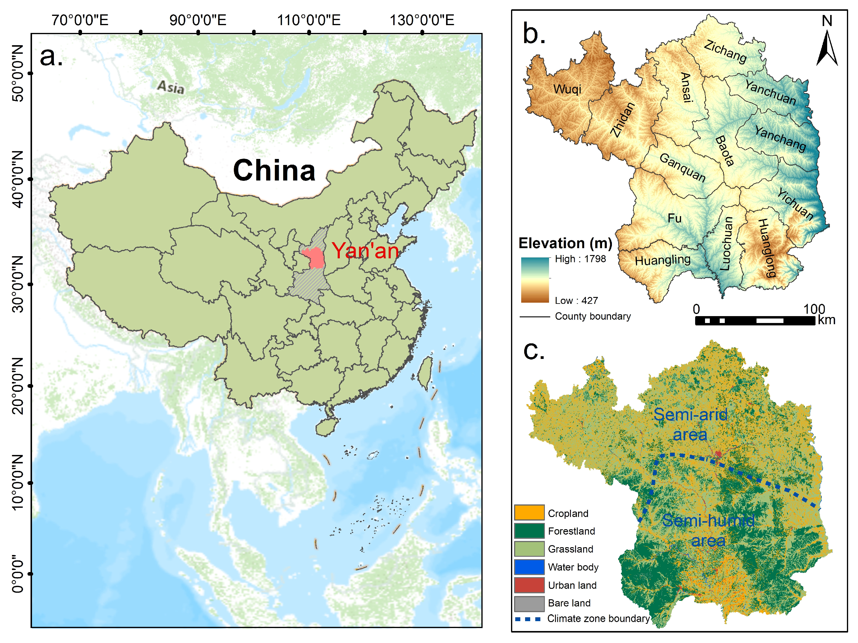
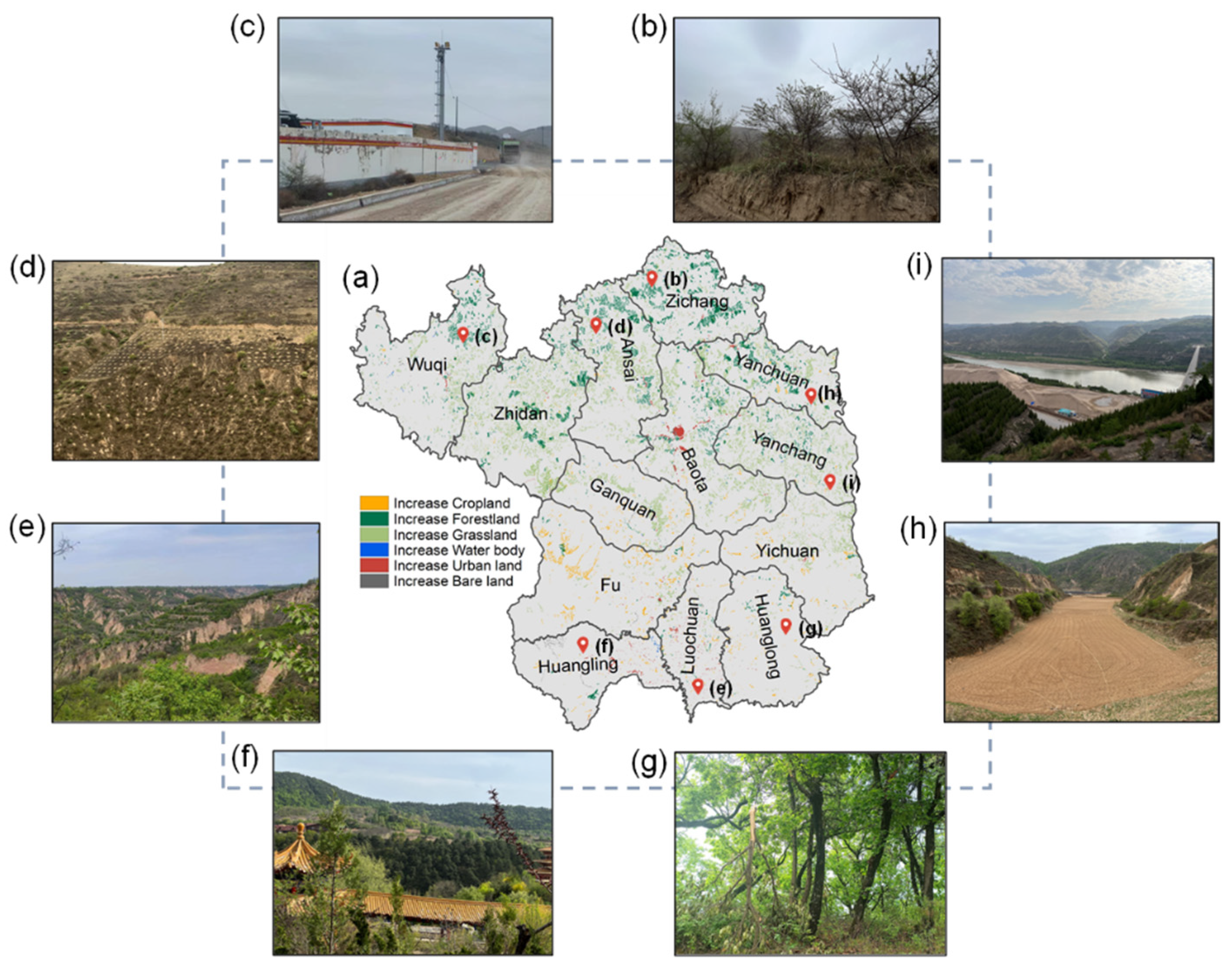
2.1. Study Area

Yan’an is located in the northern part of Shaanxi, China (35°21′ N–37°31′ N, 107°41′ E–110°31′ E) (Figure 1a). It covers a total area of 37,037 km², and is divided into 13 administrative units. Topographically, Yan’an features higher elevations in the northwest and lower elevations in the southeast, with an average elevation of approximately 1200 m (Figure 1b). According to the climate zoning in China [23], the northern part of Yan’an belongs to the semi-arid area, while the southern part belongs to the semi-humid area (Figure 1c). The annual mean temperature ranges from 10.3 to 11.6 degrees. The annual average precipitation in Yan’an is around 506 mm, primarily concentrated in July to August. Geologically, the study area belongs to the middle of hilly and rugged region on the Chinese Loess Plateau, characterized by unstable soil texture and a history of severe soil erosion.

Since the end of the last century, management measures such as small watershed management and the Grain to Green Project have been implemented in Yan’an, which have greatly contributed to the significantly increased vegetation coverage in this area. Presently, the land use structure has undergone notable changes (Figure 1c), with 21.43% of cropland being reallocated as woodland and grassland. The increased forestland is mainly in northern Yan’an, while the increased grassland is in central and southern Yan’an. In addition to re-vegetation measures, some engineering measures such as fish scale pits and check dams were implemented in northern and eastern Yan’an. Over the past 30 years, socio-economics in Yan’an has also shown consistent growth development. Fueled by abundant mineral resources, the city has experienced a steady increase in gross domestic product (i.e., GDP) and its secondary industry, reaching approximately 160.15 billion yuan and 88.57 billion yuan by 2020, respectively. However, extensive afforestation initiatives have imposed considerable pressure on local water resources, leading to instances where restored vegetation in many areas has fallen short of expectations. Moreover, the rapid economic growth has introduced uncertainties in regional environmental effects.

2.2. Research Design and Data Sources

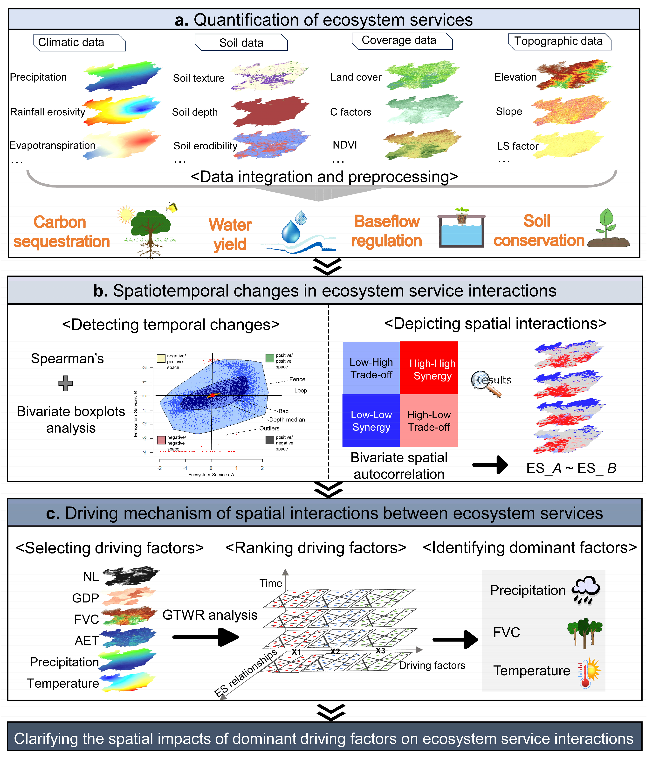
2.2.1. Research Design

The research process of this study is shown in Figure 2. Details of the map legends can be found in Supplementary Material Part I (Figure S1). Using the MODIS datasets and InVEST model, we calculated the carbon sequestration (i.e., CS), water yield (i.e., WY), baseflow regulation (i.e., BR), and soil conservation (i.e., SC) from 1990 to 2020 (Figure 2a), as they concentrated reflection on changes to the ecosystem functions under vegetation restoration. Subsequently, the Spearman correlation and bivariate boxplot analysis were applied to determine the overall temporal changes in ES interactions over the past 30 years. The spatial ES interactions and their changes were identified by using the bivariate spatial autocorrelation method (Figure 2b). Finally, the geographically and temporally weighted regression (i.e., GTWR) model was employed to explore the driving factors influencing spatial ES interactions (Figure 2c). In this process, we implemented a sorting method to identify the dominant driving factors over the past 30 years. This will offer targeted insights for improving vegetation restoration in dryland areas.

2.2.2. Data Information

In the above processes, meteorological data for this study were obtained from the National Meteorological Information Centre “https://data.cma.cn (accessed on 15 October 2022)”. Kriging interpolation was employed to transform the meteorological station data into continuously distributed spatial data, with a spatial resolution of 250 m. Soil data, utilized to quantify the soil erodibility factor and calculate the volumetric plant available water content, were obtained from the Harmonized World Soil Database (i.e., HWSD) at a spatial resolution of 1000 m “https://data.tpdc.ac.cn/ (accessed on 2 January 2023)”. The digital elevation model with a resolution of 30 m resolution was acquired from the Geospatial Data Cloud “https://www.gscloud.cn/ (accessed on 3 October 2022)”. The vegetation index was derived from the MODIS dataset “https://earthexplorer.usgs.gov/ (accessed on 4 February 2023)”, including NDVI (MOD13Q1) and NPP (MOD17A2), with spatial resolutions of 250 m and 500 m, respectively. Land use/cover data were obtained from the Institute of Geographic Sciences and Natural Resources Research, Chinese Academy of Sciences “http://www.resdc.cn/ (accessed on 27 February 2023)”, with a spatial resolution of 30 m. The land use/cover types used in this study were classified into six categories as cropland, forestland, grassland, water body, urban land, and bare land. Ecological parameters such as monthly evapotranspiration coefficients for crop (i.e., K_c) or runoff curve number (i.e., CN) are elucidated in subsequent sections. Additionally, socio-economic data, including night-time light index (500 m × 500 m) and GDP (1000 m × 1000 m), were collected for analysis of driving mechanisms. These data were all sourced from the Institute of Geographical Sciences and Natural Resources, Chinese Academy of Sciences “https://www.resdc.cn/ (accessed on 5 March 2023)”. Finally, the WGS_1984_Albers was adopted as a unified projection coordinate system. All raster data were standardized to a spatial resolution of 250 m using a nearest neighbor method to facilitate subsequent analysis.

2.3. ESs Quantification

Net primary productivity (i.e., NPP) serves as a crucial vegetation metric of the eco-logical status and productivity of terrestrial ecosystems [24]. It is commonly utilized as an indicator to reflect regional carbon sequestration dynamics [9,25]. In this study, CS was assessed using NPP as a proxy indicator, sourced from the MODIS datasets.

Based on the revised universal soil loss equation (i.e., RUSLE) [26], SC was obtained by calculating the difference between potential soil erosion and actual soil erosion. The actual soil erosion was the result of potential soil erosion multiplied by a vegetation cover factor and an erosion control practice factor [27,28]. The formula used is as follows:

$$\mathrm{SC}\left(\mathrm{x}\right)={\mathrm{E}}_{\mathrm{p}}\left(\mathrm{x}\right)-{\mathrm{E}}_{\mathrm{a}}\left(\mathrm{x}\right)$$

(1)

$${\mathrm{E}}_{\mathrm{a}}=\mathrm{R}\left(\mathrm{x}\right) \times \mathrm{K}\left(\mathrm{x}\right) \times \mathrm{LS}\left(\mathrm{x}\right) \times \mathrm{C}\left(\mathrm{x}\right) \times \mathrm{P}\left(\mathrm{x}\right)$$

(2)

$${\mathrm{E}}_{\mathrm{P}}\left(\mathrm{x}\right)=\mathrm{R}\left(\mathrm{x}\right) \times \mathrm{K}\left(\mathrm{x}\right) \times \mathrm{LS}\left(\mathrm{x}\right)$$

(3)

where E_a(x) and E_p(x) refer to actual and potential soil erosion in pixel x, respectively; R(x) is the rainfall erosion factor. The R factors in 1990, 2000, 2010, and 2020 were calculated based on the monthly rainfall [29]. The erosion productivity impact calculator (i.e., EPIC) equation was applied to calculate the soil erosion factor (i.e., K factor) [30], in which the contents of sand, silt, clay, and organic carbon were obtained from the HWSD. LS(x) is the slope length factor calculated from DEM. The C(x) is the vegetation cover factor in pixel x, and the P(x) is the erosion control practice factor in pixel x. They were estimated by using a fractional vegetation cover-based method [28] and a slope-based method [31], respectively.

Then, the InVEST water yield model, utilizing the principle of water balance to estimate the depth of WY in each grid cell, was applied. The detailed theory can be found in the InVEST User’s Guide. The formula employed is as follows:

$$\mathrm{Y}(\mathrm{x}) =\left[1-\frac{\mathrm{AET}\left(\mathrm{x}\right)}{\mathrm{P}\left(\mathrm{x}\right)}\right]\times \mathrm{P}(\mathrm{x})$$

(4)

$$\frac{\mathrm{AET}\left(\mathrm{x}\right)}{\mathrm{P}\left(\mathrm{x}\right)}=1+\frac{\mathrm{AET}\left(\mathrm{x}\right)}{\mathrm{P}\left(\mathrm{x}\right)}-{\left[{\left(1+\frac{\mathrm{AET}\left(\mathrm{x}\right)}{\mathrm{P}\left(\mathrm{x}\right)}\right)}^{\mathsf{\omega }}\right]}^{\raisebox{1ex}{$1$}\!\left/ \!\raisebox{-1ex}{$\mathsf{\omega }$}\right.}$$

(5)

$$\mathrm{PET}\left(\mathrm{x}\right)={\mathrm{K}}_{\mathrm{c}}({\mathrm{l}}_{\mathrm{x}}) \times {\mathrm{ET}}_0\left(\mathrm{x}\right)$$

(6)

$$\mathsf{\omega }(\mathrm{x})=\mathrm{Z}\frac{\mathrm{AWC}\left(\mathrm{x}\right)}{\mathrm{P}\left(\mathrm{x}\right)}+1.25$$

(7)

where Y(x) is the water yield in pixel x; AET is the actual evapotranspiration; P(x) is the precipitation in pixel x, and the precipitation layers are mapped by spatial interpolation based on the meteorological station data (Table 1); PET(x) is the potential evapotranspiration; K_c(l_x) is the crop evapotranspiration correlation coefficient. Using the modified Hargreaves equation, the annual reference evapotranspiration (i.e., ET₀(x)) in 1990, 2000, 2010, and 2020 were quantified [32]. The ω(x) is an empirical parameter; AWC(x) is the volumetric plant available water content. The soil parameters were also obtained from the HWSD and were used to calculate the volumetric plant available water content (i.e., PAWC). The Z parameter is an empirical constant reflecting the seasonal distribution of precipitation ranging from 1 to 30. Using the empirical formula based on the number of precipitation events in each year [33], we calculated the Z values as 20.26, 17.13, 20.4, and 19.47, respectively.

BR is the discharge from underground storage and can be the main source of streamflow in the dry season [34]. The InVEST seasonal water yield model was used to quantify this service. Monthly precipitation and monthly evapotranspiration data were mapped for each year. Meanwhile, we counted the number of monthly precipitation events in 1990, 2000, 2010, and 2020, respectively, to create a CSV table for the model input. The hydrological soil group was classified based on soil texture derived from the HSWD. Values of K_c were readily available from the InVEST online resources “https://naturalcapitalproject.stanford.edu/software/invest/invest-downloads-data (accessed on 22 January 2023)”. It is calculated as follows:

$${\mathrm{QF}}_{\mathrm{i},\mathrm{m}}={\mathrm{RE}}_{\mathrm{i},\mathrm{m}}\times \left\{\left({\mathrm{a}}_{\mathrm{i},\mathrm{m}}-{\mathrm{S}}_{\mathrm{i}}\right)\exp \left(-\frac{0.2{\mathrm{S}}_{\mathrm{i}}}{{\mathrm{a}}_{\mathrm{i},\mathrm{m}}}\right)+\frac{{\mathrm{S}}_{\mathrm{i}}^2}{{\mathrm{a}}_{\mathrm{i},\mathrm{m}}}\exp \left(\frac{0.8{\mathrm{S}}_{\mathrm{i}}}{{\mathrm{a}}_{\mathrm{i},\mathrm{m}}}\right){\mathrm{E}}_1\left(\frac{{\mathrm{S}}_{\mathrm{i}}}{{\mathrm{a}}_{\mathrm{i},\mathrm{m}}}\right)\right\}\times \left(25.4\left[\frac{\mathrm{mm}}{\mathrm{in}}\right]\right)$$

(8)

where QF_i,m, RE_i,m, and a_i,m are, respectively, the quick flow generated by pixel i in month m, the number of rain events, and the mean rain depth. The irrigation and horticulture handbooks published by FAO to determine the CN value for each soil group, were used to calculate S_i:

$${\mathrm{L}}_{\mathrm{i}}={\mathrm{P}}_{\mathrm{i}}-{\mathrm{QF}}_{\mathrm{i}}-{\mathrm{AET}}_{\mathrm{i}}$$

(9)

where L_i is the local recharge derived from the annual water budget; P_i is the annual precipitation; AET_i is the annual actual evapotranspiration.

If the local recharge is negative, the pixel does not contribute to baseflow and is assigned 0. If the pixel contributed to groundwater recharge, then it is a function of the amount of flow leaving the pixel and of the relative contribution to recharge of this pixel. For a pixel that is not adjacent to the stream channel, the cumulative baseflow is proportional to the cumulative baseflow that leaves the adjacent downslope pixels minus the cumulative baseflow generated on the same downslope pixel:

$${\mathrm{B}}_{\mathrm{sum},\mathrm{i}}={\mathrm{L}}_{\mathrm{sum},\mathrm{i}}, \mathrm{if} \mathrm{j} \mathrm{is} \mathrm{a} \mathrm{nonstream} \mathrm{pixel}$$

(10)

$$\mathrm{or} {\mathrm{B}}_{\mathrm{sum},\mathrm{i} }{=\mathrm{L}}_{\mathrm{sum},\mathrm{i}}{\sum }_{\mathrm{j}\in \left\{\mathrm{cells} \mathrm{to} \mathrm{which} \mathrm{cell} \mathrm{i} \mathrm{pours}\right\}}{\mathrm{P}}_{\mathrm{ij}}, \mathrm{if} \mathrm{j} \mathrm{is} \mathrm{a} \mathrm{stream} \mathrm{pixel}$$

(11)

$${\mathrm{B}}_{\mathrm{i}}=\max \left({\mathrm{B}}_{\mathrm{sum},\mathrm{i}}·\frac{{\mathrm{L}}_{\mathrm{i}}}{{\mathrm{L}}_{\mathrm{sum},\mathrm{i}}}\right),0$$

(12)

where B_sum,i is the actual contribution of a pixel to the baseflow; L_sum,i is the cumulative upstream recharge; p_ij is the proportion of flow from cell i to j. And baseflow B_i, can be directly derived from the proportion of the cumulative baseflow leaving cell i, with respect to the available recharge to the upstream cumulative recharge.

The four ESs were all mapped in ArcGIS 10.5 to visualize their spatial patterns in 1990, 2000, 2010, and 2020. Their overall changes over the past 30 years were also provided to facilitate subsequent analysis (Supplementary Material Part II).

2.4. Integrated Approach for Detecting ESs Interactions

2.4.1. Detecting Temporal Changes in ES Relationships

In this study, the Spearman analysis was applied to describe the average states of ES interactions. It can be expressed as follows:

$${\mathrm{r}}_{\mathrm{s}}=1-\frac{6\sum {\mathrm{d}}_{\mathrm{i}}^2}{\mathrm{N}({\mathrm{N}}^2-1)}$$

(13)

$${\mathrm{d}}_{\mathrm{i}}={\mathrm{X}}_{\mathrm{i}}-{\mathrm{Y}}_{\mathrm{i}}$$

(14)

where r_s is the rank correlation coefficient, ranging from −1 to 1, N refers to the total number of samples, X_i and Y_i, respectively, represent the serial numbers of two datasets that have been arranged from smallest to largest, d_i refers to the difference of each team sorting variable. To perform the statistical analysis, we spatially sampled four ESs in each period. The Z-score standardized method was employed to normalize the 6000 sample points. Then, the Spearman analyses for all pairs of ESs were calculated in R v4.2.2. Referring to the relevant research [17], correlation coefficients of Spearman were divided as high correlation (|r| ≥ 0.5), moderate correlation (0.3 ≤ |r| ≤ 0.5), and low correlation (0.1 ≤ |r| ≤ 0.3). A significant positive correlation indicates a synergic relationship between the two ESs, while a significant negative correlation suggests a trade-off between them.

The bivariate boxplot, a non-parametric statistical method, was then employed to delineate the asymmetry and discrete correlations among ESs [35]. Bagplot provides a visual representation of the interaction between two variables [36]. The position of the depth median in the bagplot identifies the area where the data are relatively concentrated [37]. Combining bag direction (correlation), bag shape (distribution asymmetry and outliers), and bag area (discretization of data distribution) enables a better understanding of the relationship between ESs (Figure 2b). In this study, we plotted the bagplots for ES pairs using the ‘aplpack’ package in R v4.2.2.

2.4.2. Spatially Explicit Analysis on ES Interactions

The bivariate spatial autocorrelation was employed to reveal the spatial interactions between two ESs. This method can quantify relationships between two variables with spatially interactive characteristics, thereby helping to reveal potential connections among ESs. It comprises the global spatial autocorrelation and the local spatial autocorrelation. The former reflects whether the ES interactions are spatially correlated across the entire study area, typically quantified using the global Moran index (i.e., Moran’s I). Local spatial autocorrelation examines the correlation between one variable at a specific location with another variable at the neighboring location, often represented using a local indicators of spatial association (i.e., LISA) cluster [38]. Hence, trade-off and synergy between two ESs can be visualized by analyzing the LISA cluster types [39]. In other words, synergy or trade-off can be identified based on codirectional correlation (i.e., ‘high–high’ or ‘low–low’ interaction) or the inverse correlation (i.e., ‘high–low’ or ‘low–high’ interactions) in the LISA cluster maps (Figure 2b).

Here, the global Moran’s I and local LISA cluster plots for each ES pair in 1990, 2000, 2010, and 2020 were calculated using the GeoDa1.10 software. This software has been widely used in geospatial data analysis to explore in-depth potential patterns, trends, and correlations in geographic space [38]. We created grids with 2500 m × 2500 m in ArcGIS10.5 as the survey unit for mapping the LISA cluster between ESs. This grid scale can satisfy the load for computer running and also provide more granular ES interaction information. It should be pointed out that the spatial autocorrelation of variables is a prerequisite for the application of the LISA and the GTWR analysis in subsequent sections. Thus, we examined the suitability for the ES interactions using the global Moran’s I. The p-value of the global Moran’s I represents the probability of this trend occurring, and the Z-score is a multiple of the standard deviation [40]. According to the test standards (Table S2), the six ES pairs from 1990 to 2020 all passed the significance test with high degree of confidence (Table S3). This process demonstrates the applicability of LISA in this study.

2.5. Analyzing the Spatial Driving Factors of ES Interactions

2.5.1. Theory on the GTWR Model

This study used the GTWR model to explore the driving mechanism on the ES interactions over the past 30 years (Figure 2c). The GTWR is a local linear regression model that incorporates spatiotemporal non-stationarity, in which each observation possesses a unique temporal weight matrix. And the regression coefficient of observations to the dependent variable attenuates with the increasing distance in time and space [41]. As an extension for the GWR, this method not only captures the comprehensive spatial information of driving factors, but also addresses the issue of their time-scale variations, providing more accurate results in time series analysis [42]. The formula of the GTWR model can be expressed as follows:

$${\mathrm{y}}_{\mathrm{i}}={\mathsf{\beta }}_0({\mathrm{u}}_{\mathrm{i}},{\mathrm{v}}_{\mathrm{i}},{\mathrm{t}}_{\mathrm{i}})+{\sum }_{\mathrm{k}=1}^{\mathrm{p}}{\mathsf{\beta }}_{\mathrm{k}}({\mathrm{u}}_{\mathrm{i}},{\mathrm{v}}_{\mathrm{i}},{\mathrm{t}}_{\mathrm{i}}){\mathrm{x}}_{\mathrm{i}\mathrm{k}}+{\mathsf{\epsilon }}_{\mathrm{i}}$$

(15)

where y_i is the explanatory variable for the i-th sample; u_i, v_i, t_i refer to the latitude, longitude, and data time of the i-th sample, respectively; β₀(u_i, v_i, t_i) refers to the regression intercept; β_k(u_i, v_i, t_i) refers to the regression coefficient of the variable k; x_ik is the value of variable x_k at i sample; and ε_i is the residual of the model.

2.5.2. Selection of Driving Factors

The direct ecological processes and the external ’catalysis’ by nature or socio-economics are commonly regarded as the two types of reasons for ES trade-offs and synergies [43,44]. Consulting relevant studies in Table 1, we initially collected nine major indicators for the GTWR analysis. The GTWR method emphasizes spatial variations of variables over time [22]. Changes in terrain factors were generally weak on the 30-year time scale, thus, they were consequently not included in the final analysis. Furthermore, the multicollinearity should be removed to avoid information redundancy among variables. Here, the variance inflation factor (i.e., VIF) was used to test the multicollinearity among driving factors. In this process, population density was excluded based on the results of multicollinearity tests. Ultimately, six driving factors (Table 1), including temperature, precipitation, actual evapotranspiration (i.e., AET), fractional vegetation cover (i.e., FVC), GDP, and night-time light index were selected to determine the impacts on ES trade-offs and synergies. The results of VIF for the six variables in each year are shown as

Table 2. VIF test for driving factors.

Variables	VIF Results
	1990	2000	2010	2020
Temperature	1.6	2.5	6.4	3.7
Precipitation	3.5	6.0	10.5	6.4
AET	6.5	7.7	5.4	3.7
FVC	5.6	5.3	5.0	3.5
GDP	1.2	1.2	1.4	1.1
Night-time light index	1.1	1.1	1.2	1.1

. All values were below 10, suggesting there was no multicollinearity among these factors [45].

Table 1. Selection of driving factors of ES interactions.

Types	Variables	References
Meteorological factors	Temperature	[46,47,48]
	Precipitation
	AET
Vegetation factors	FVC	[49]
Terrain factors	Elevation	[5,50]
	Slope
Socio-economic factors	GDP	[51]
	Night-time light index	[52]
	Population density

Note: the black variables denote the factors that were ultimately incorporated into the GTWR model, whereas the italicized grey variables represent factors that were excluded in the analysis as they did not meet the research requirements.

Table 1. Selection of driving factors of ES interactions.

Types	Variables	References
Meteorological factors	Temperature	[46,47,48]
	Precipitation
	AET
Vegetation factors	FVC	[49]
Terrain factors	Elevation	[5,50]
	Slope
Socio-economic factors	GDP	[51]
	Night-time light index	[52]
	Population density

Note: the black variables denote the factors that were ultimately incorporated into the GTWR model, whereas the italicized grey variables represent factors that were excluded in the analysis as they did not meet the research requirements.

2.5.3. Model Execution and Goodness Detection

We performed the GTWR model using ArcGIS10.5. The Gaussian distance–decay-based function was used to calculate the spatiotemporal weights. The corrected Akaike information criterion (i.e., AICc) was utilized to determine the optimal bandwidth. Subsequently, we examined the advantages of GTWR compared to the GWR using representative statistical indices. The R² value indicates the goodness of fit of the independent variables to the dependent variable. The AICc measures the balance between the accuracy of different models and the number of calibration parameters, with lower values indicating better model performance [53]. The comparison results indicates that the latter had a better fitting effect (

Table 3. Comparison of goodness between the GWR and the GTWR models.

ES Pairs	Model	R2	AICc
CS-WY	GTWR	0.74	920.3
	GWR	0.63	978.7
BR-WY	GTWR	0.79	1181.0
	GWR	0.71	1240.7
BR-CS	GTWR	0.69	1280.6
	GWR	0.64	1272.7
SC-CS	GTWR	0.68	1295.0
	GWR	0.62	1294.7

).

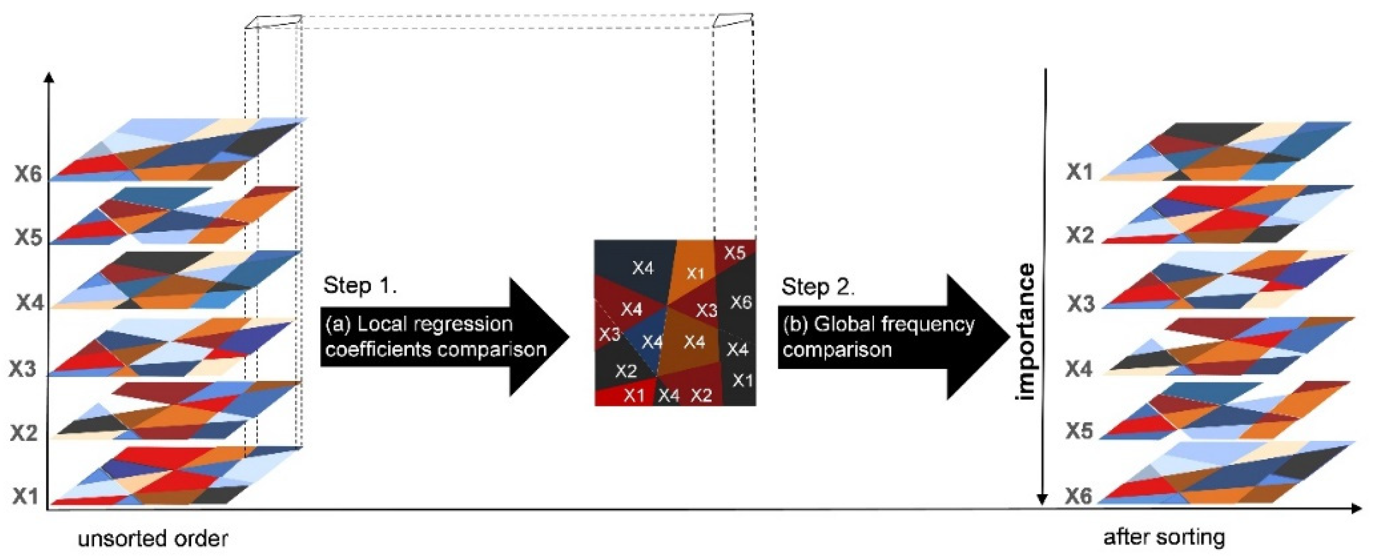
2.5.4. Ranking the Driving Factors to Discern Dominant Factors in Each Period

Changes in direction and strength of influence are generally the two important aspects for detecting driving mechanisms [41,54]. The GTWR results presented maps of spatial regression coefficients for each driving factor over the past 30 years. However, these coefficients exhibited variations both in strength and direction across space, making it difficult to determine directly the dominant drivers on ES interactions in each location.

Here, we implemented a ranking approach to identify the dominant driving factors based on the spatial regression coefficients of the six factors (Figure 3). First, we conducted a ranking by comparing the absolute values of the normalized regression coefficients for each driving factor. That is, the one with the largest regression coefficient was regarded as the first driving factor for the analyzed unit, and so forth. This process eliminated the interferences of the sign (i.e., direction) of coefficients on their strength. Based on the preceding step, we sequentially calculated the frequency of occurrence from the first to sixth driving factors across the entire study area. The driving factor with the highest frequency was identified as the primary driving force, followed by the subsequent factors in descending order, ultimately establishing the final ranking of the driving factors. Consequently, integrating local regression coefficients and global frequencies, the ranking approach offers a comprehensive reflection of the importance of driving factors. This highlighted those factors likely to have a particularly strong impact on the ES relationships. It should be emphasized that we just screened out the dominant driving factors through the ranking approach. Thus, the later section showed the original results obtained from the GTWR model.

3. Results

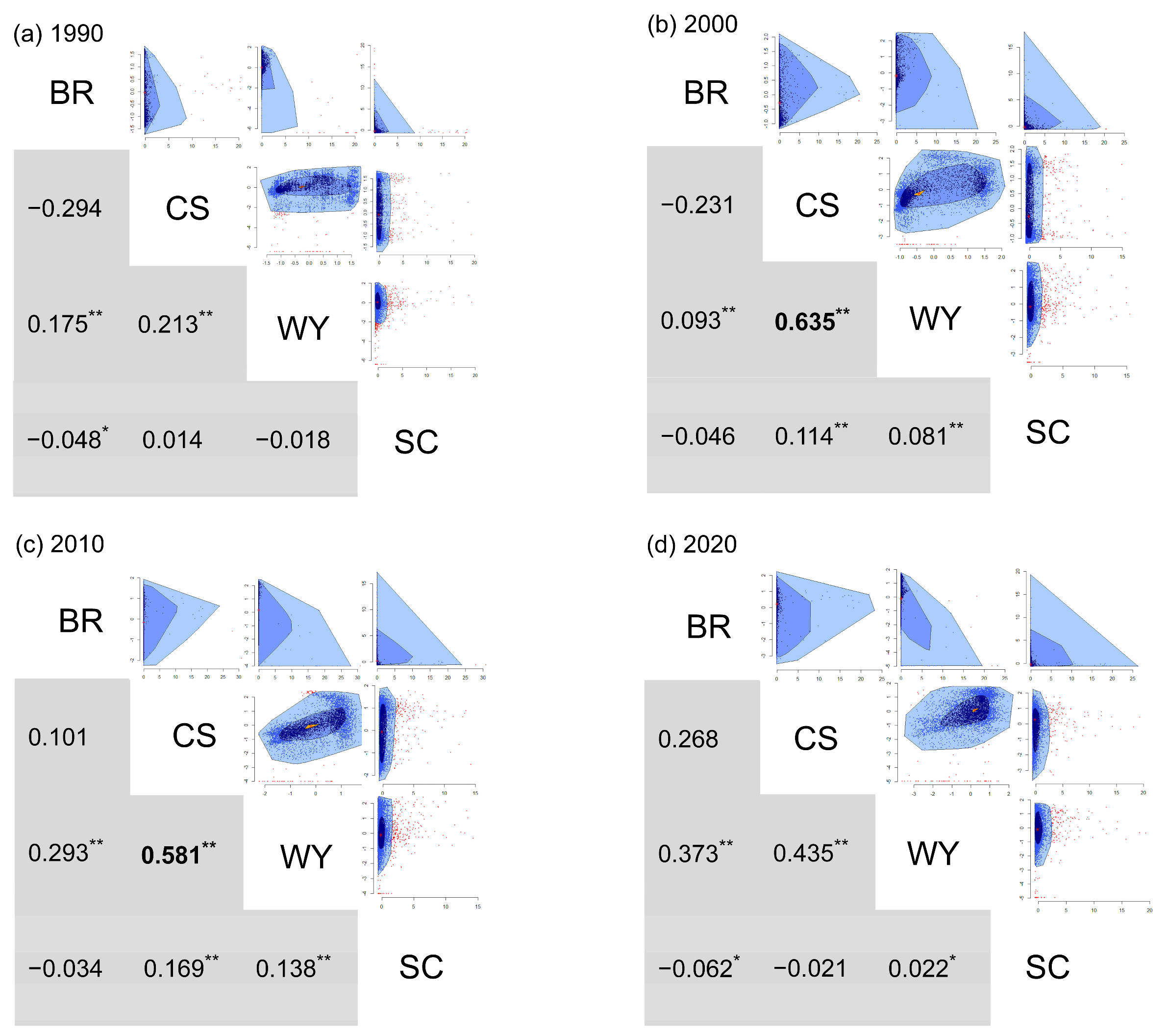
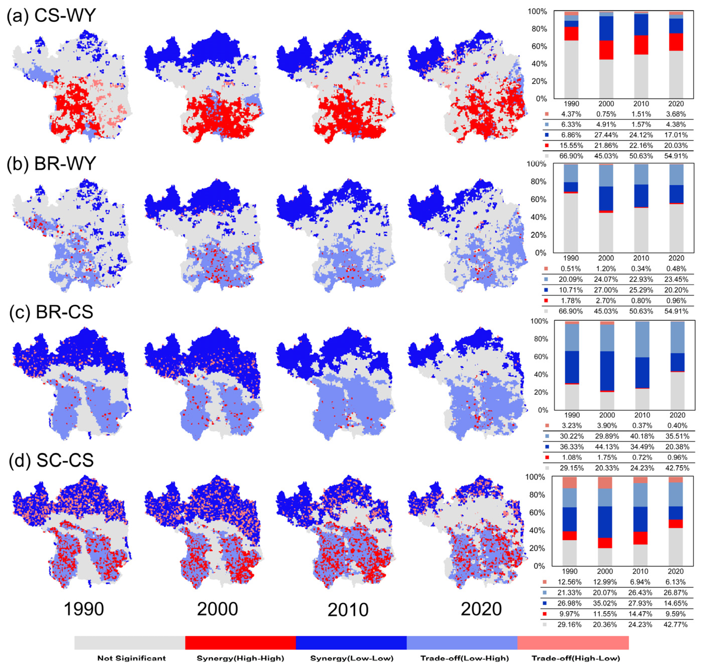
3.1. Temporal Changes in ES Interactions

The combined results of Spearman correlation and bivariate boxplot analysis indicated changes in the interactions between ES pairs over time (Figure 4). In 1990, only three of the six ES pairs showed statistically significant correlations, all of which were weakly correlated (0.1 ≤ |r| ≤ 0.3). After 2000, the significant synergistic relationships were concentrated among CS, WY, and SC, demonstrating an overall increase compared with 1990. However, synergies between CS and WY have gradually weakened over the past 20 years. Moreover, correlation between WY and SC, as well as CS and SC, reached their maximum in 2010, followed by a declining trend in the last decade. A significant synergy was observed between BR and WY, while relationships between BR and the other two ESs were always very faint over the past 30 years.

The bagplots offered detailed information on the interaction types among the four ESs. For the synergy between CS and WY in 1990 (Figure 4a), data values were concentrated in the high-value region along the CS axis, running almost parallel to the WY axis. This suggested that the synergistic relationship between the two ESs was primarily driven by areas with high CS values. From 2000 to 2010 (Figure 4b,c), however, the concentrated values in bagplots emerged at both ends of the bags, suggesting the synergies between the two ESs were contributed by both high-value CS areas and low-value CS areas. In contrast, bagplots of CS and SC, as well as WY and SC, exhibited an approximately vertical distribution over the past 30 years. This implied that the synergies were mainly contributed by the low-value areas of SC. The bagplots of BR and other ESs showed a triangle and a larger area of loop, representing the numerical discreteness in this service. And the distribution of concentrated values indicated that the weak synergies related to BR and other ESs were mainly contributed by the low values of BR.

3.2. Spatial Variations in ES Interactions

Water consumption during the growth stages of restored vegetation varies depending on natural conditions and vegetation types, largely leading to the differences in carbon and water related ESs within a region [55]. Based on the results of bivariate spatial autocorrelation, we exhibited the spatial interactions of ES pairs, including carbon sequestration and water yield (i.e., CS-WY), baseflow regulation and water yield (i.e., BR-WY), baseflow regulation and carbon sequestration (i.e., BR-CS), soil conservation and carbon sequestration (i.e., SC-CS). Indeed, these four ES pairs highlighted two distinct spatial interactions (Figure 5), revealing the spatial differentiation of trade-offs and synergies in the northern and southern areas.

First, the spatial interaction patterns of CS-WY and BR-WY had similar features (Figure 5a,b). It can be observed that the two ES pairs manifested ‘low–low’ synergy in the northern semi-arid areas, with an initially increased area followed by a decrease. In the southern semi-humid counties, the two ES pairs also showed consistency in their spatial distribution. However, CS-WY displayed the ‘high–high’ synergy, whereas BR-WY showed ‘low–high’ trade-off, with the proportion exceeding 20%. It indicated these regions had higher WY accompanied by lower BR. Second, BR-CS and SC-CS shared the similar spatial interaction patterns, exhibiting ‘low–low’ synergy in the northern semi-arid areas (Figure 5c,d). Interactions of the two ES pairs also showed differences in the southern counties. The ‘low–high’ trade-off was evident in BR-CS, primarily distributed in native vegetation areas in the southeast and southwest counties. In contrast, SC-CS showed a certain area of ‘high–high’ synergy in the southern counties, peaking at 14.47% in 2010.

3.3. Spatial Driving Mechanism of ES Interactions

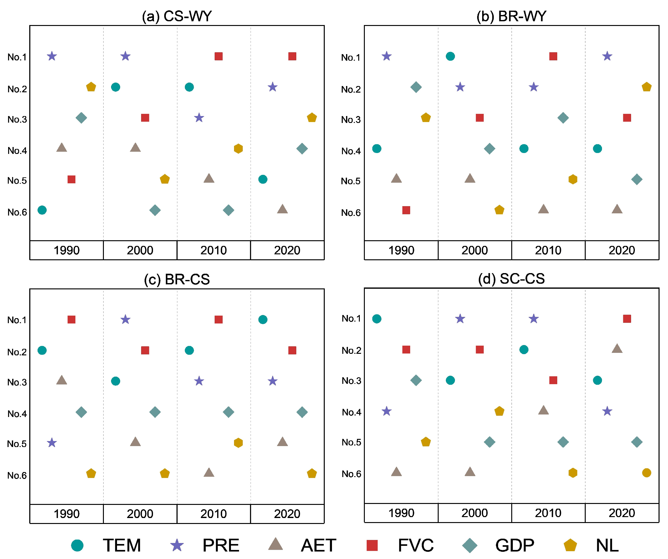
3.3.1. Driver Changes in ES Interactions

Figure 6 illustrated the ranking of driving factors affecting the four types of ES interactions at different periods. For the CS-WY and the BR-WY (Figure 6a,b), precipitation emerged as a primary factor, consistently ranking a position in the top three over the past 30 years. Human activities, including night-time light index and GDP, also played a dominant role before the vegetation restoration, reflecting the high sensitivity of ecosystem functions to human disturbance. From 2000 to 2010, FVC became the dominant driver, and its contribution continued to increase during this period. Meanwhile, impacts stemming from GDP and night-time light index have weakened since 2000. Over the last decade, the increased forestlands and grasslands have gradually stabilized under artificial management and natural regulation, while the contribution of human activities has been on the rise.

Temperature and FVC have been the dominant driving factors for BR-CS and SC-CS (Figure 6c,d), consistently ranking among the top three factors. In 1990, the impact of precipitation was comparatively weak. After 2000, while the effects of precipitation showed fluctuating changes, its overall contributions to BR-CS increased. Accordingly, FVC and temperature, along with precipitation determined the changes in the ES relationships from 2000 to 2020. Meanwhile, contributions from AET exhibited a continuous upward trend for SC-CS, reaching the second position in 2020. However, GDP or night-time light index exerted stable and minor impacts on the two types of ES pairs over the past 30 years.

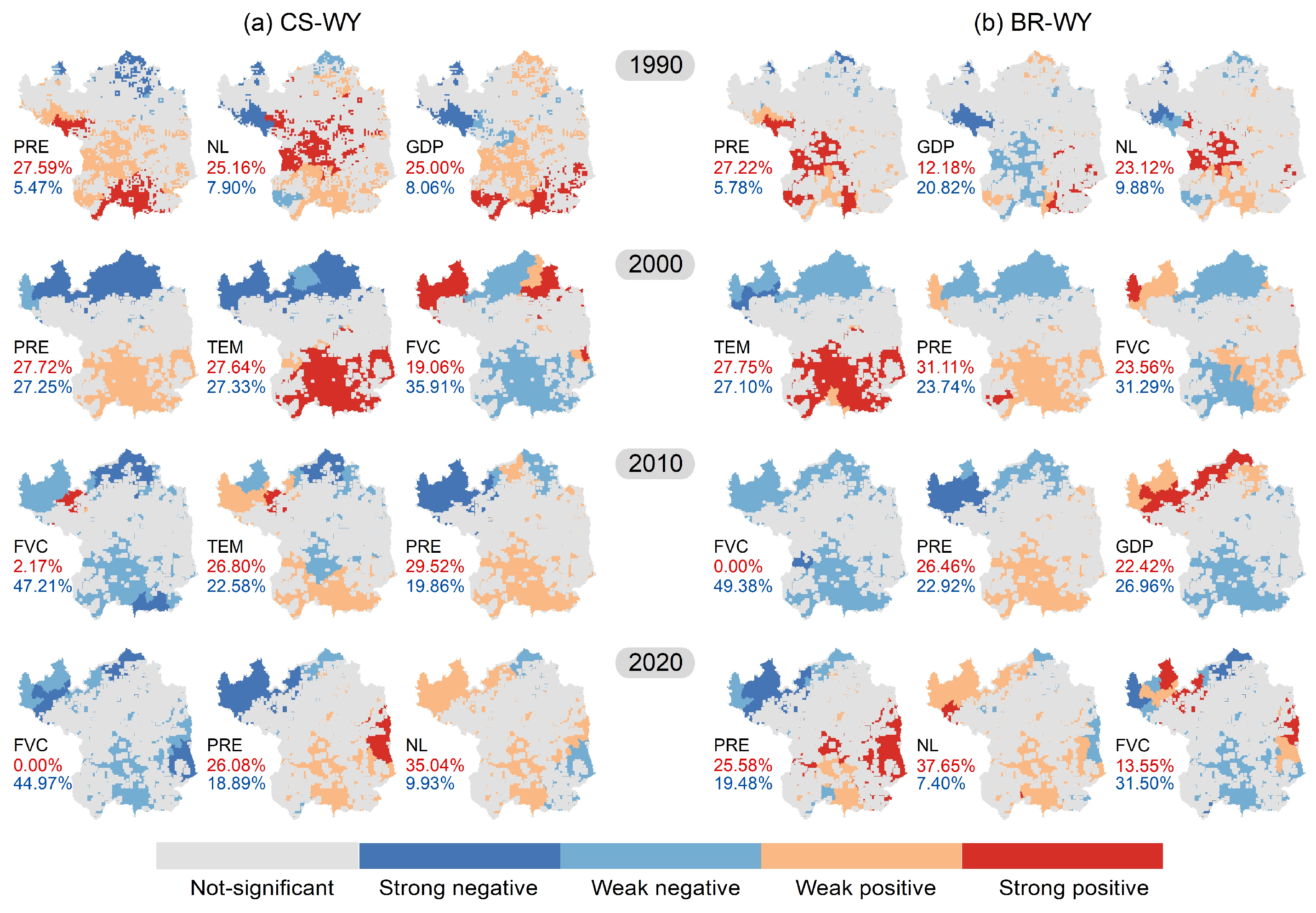
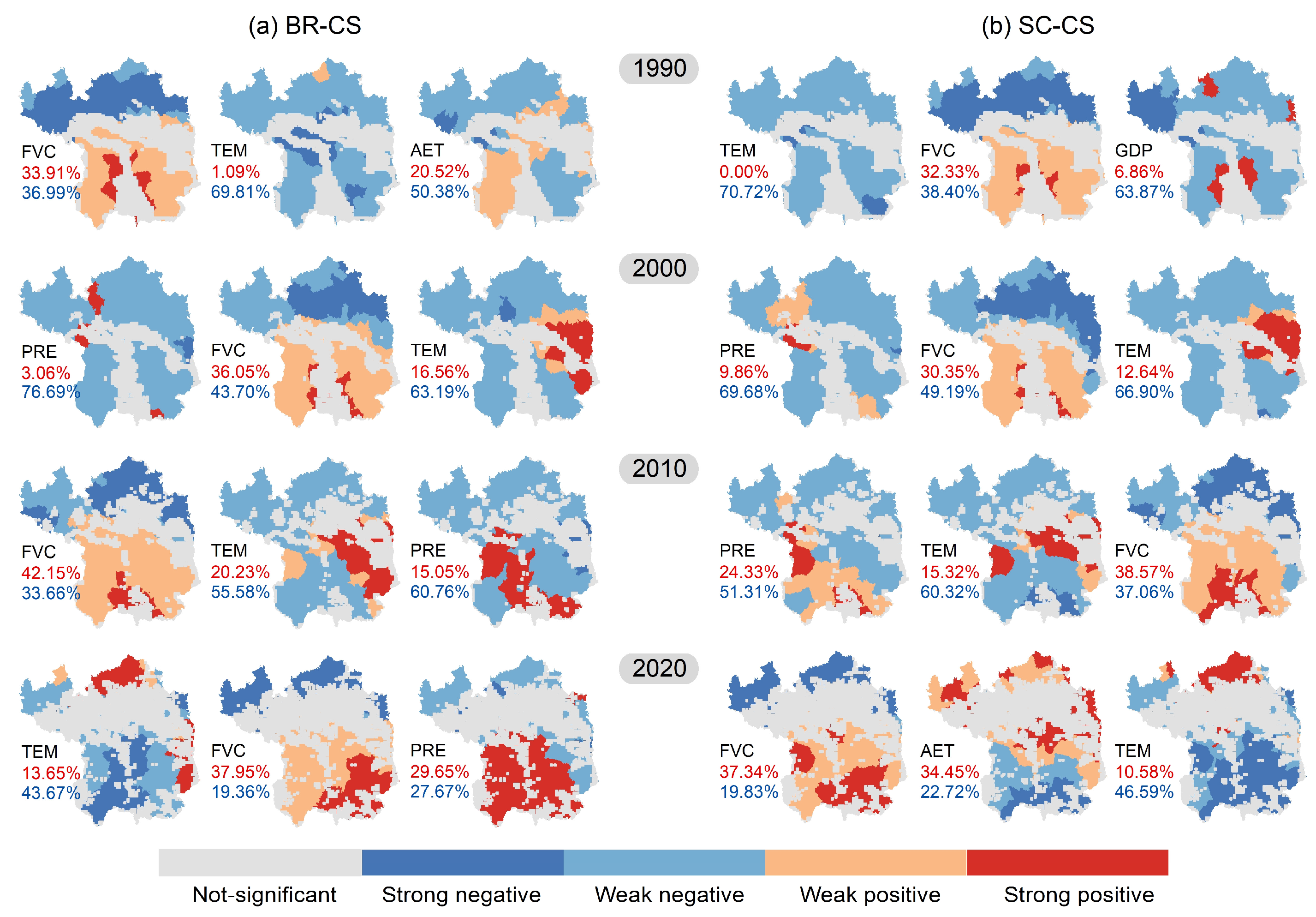
3.3.2. Spatial Changes in Driving Factors of ES Interactions

Here, the dominant driving factors of the four ES pairs were mapped (Figure 7 and Figure 8). In general, the spatial dominant driving factors of CS-WY and BR-WY exhibited consistency. A comparable picture was also observed for BR-CS and SC-CS.

For CS-WY, the results revealed the effects of spatial drivers on different types of synergies between the two ESs in the northern and southern areas (Figure 7a). Precipitation negatively affected the ‘low–low’ synergy of CS-WY in the northern semi-arid areas, but had a positive effect on the ‘high–high’ synergy in the central-southern semi-humid areas. Notably, as the impacts of FVC increased (Figure 6a), its positive effects on CS-WY decreased from 19.06% to 2.17% from 2000 to 2010. By 2020, FVC exhibited entirely negative impacts on CS-WY, with more pronounced negative effects in the northern areas. Furthermore, in 1990, both GDP and night-time light index had adverse effects on the ‘low–low’ synergy in the northern regions, and exhibited positive effects in the southern counties. However, in the last decade, night-time light index demonstrated positive impacts (accounting for 35.04%) in most areas of the study area.

The spatial impacts of precipitation and FVC on BR-WY exhibited patterns similar to their effects on CS-WY (Figure 7b). However, precipitation may exacerbate the ‘low–high’ trade-off in southern counties. Meanwhile, the positive impact area of FVC on the ‘low–high’ trade-off in BR-WY decreased from 23.56% to 13.55% from 2000 to 2020, accompanied by a significant shift of positive impacts on location. Compared to 2000, for instance, FVC exhibited its negative impacts on the south counties in 2020. Additionally, the impact pattern of night-time light index on BR-WY was almost the same as that of CS-WY in 2020, with a positive impact area of 37.65%.

Overall, FVC, temperature, and precipitation exhibited comparable spatial influence patterns on the BR-CS and SC-CS (Figure 8). In the northern semi-arid areas, the ‘low–low’ synergy was suffered mainly from precipitation, temperatures and FVC negative effects (Figure 8a). By contrast, the positive effects of FVC and precipitation on the ‘low–high’ trade-off of BR-CS consistently expanded after 2000, reaching a proportion of 37.95% and 29.65% in 2020. In other words, the increases in FVC and precipitation would intensify the trade-offs between BR and CS. By 2020, AET exhibited a stronger influence on SC-CS, as depicted in Figure 8b. This influence manifested positively in the northern region but negatively impacted on the SC-CS in southern counties, accounting for 34.45% and 22.72%, respectively.

4. Discussion

4.1. Differentiated Synergies among ESs under Vegetation Restoration

Trade-off theory that more vegetation leads to less water has become a prevailing paradigm in recent decades [56,57]. However, conclusions on carbon and water-related ES relationships resulting from re-vegetation in drylands often vary across the scientific literature. Many regional-scale studies also verify that vegetation restoration enhances the synergistic benefits between CS and water-related ESs [58,59]. Therefore, adopting an explicit perspective that considers both temporal and spatial changes is equally crucial for analyzing ES interactions [60]. Through the long-term scale analysis on ES spatial interactions in this study, the results revealed the distinctly different synergistic effects between carbon and water-related ESs in semi-arid areas and semi-humid areas. This offers important insights for clarifying previous ambiguous information.

Over the past 30 years, the increase in forestland and grassland in Yan’an has been primarily concentrated in the northern areas of Wuqi, Zichang, Zhidan, and Ansai, as well as in the southern regions of Fu and Luochuan (Figure 9a). Changes in trade-offs and synergies of CS-WY and BR-WY have been indeed concentrated in these counties, indicating the sensitivity of water-related ESs to vegetation restoration. Despite extensive reforestation efforts in the northern regions, the accumulated biomass remained lower. Meanwhile, the arid climate conditions have led to a lower WY and BR in the northern counties. In contrast, WY in the southern counties has been always the highest in the region due to the abundant rainfall. Consequently, the patterns of the ‘low–low’ synergy in the northern counties and the ‘high–high’ synergy in the southern counties collectively contributed to the positive relationships between CS and WY over the past 30 years (Figure 4).

During field surveys, we found that the recovery grasslands in the southern counties typically manifested in the form of ‘patches’ intricately interwoven within the original natural or secondary vegetation communities (Figure 9e). However, the efficiency of recovery grasslands for preventing soil loss and promoting water infiltration is notably inferior to that of the surrounding perennial tree vegetation [61]. Moreover, Luochuan and Fu have been the main counties for cropland utilization in the southern region, presenting an increased area of croplands over the past 10 years. The loose soil resulting from agricultural activities coupled with abundant rainfall renders these areas more prone to soil erosion [62]. Consequently, the spatial mismatch between higher WY and lower SC or BR in southern counties resulted in the spatial patterns of ‘low–high’ trade-off for SC-WY or BR-WY (Figure 5b).

However, the ‘low–high’ trade-offs in BR-CS and SC-CS were completely different in the native vegetation areas in the southeast (i.e., Yichuan and Huanglong) and southwest (i.e., Fu and Huangling). In regions with a high cover of native vegetation (Figure 9f), the penetration of vegetation roots effectively stabilizes the soil and prevents soil erosion [63]. Meanwhile, the densely staggered canopy directly intercepts precipitation and stores it within the plant canopy for subsequent evaporation, resulting in less water infiltration into the ground [46]. Therefore, the ‘low–high’ trade-offs of BR-CS reflect the direct interactions of ecosystem functions rather than the deterioration of ESs (Figure 5c). Additionally, the synergy of SC-CS in mature forests has been widely demonstrated in numerous studies [64]. However, this study further revealed that in the later growth stage of mature forests, the ‘high–high’ synergy area of SC-CS decreased to 9.59% (Figure 5d). According to the field surveys, thinning may be one of the reasons. Coincidentally, recent research also indicated that CS and SC exhibited trade-off interactions under the combined influences of climate and vegetation change [65]. These insights all emphasized the necessity to analyze ES interactions based on local drivers.

4.2. Driving Forces with Spatial Differences Jointly Affect ES Interactions

Time lags in ES responses caused by vegetation growth or climate changes, along with the spatial heterogeneity of ESs induced by spatial isolation or human activities, contribute to the intricate interactions of the ESs [12,66]. This study revealed that the interactions among carbon, water, and soil related ESs have been primarily driven by FVC, precipitation, and temperature, and exhibited spatially differentiated effects in northern and southern areas (Figure 7 and Figure 8).

In an arid climate environment, increased FVC and temperature directly aggravate vegetation water consumption and water evaporation [67], resulting in reduced WY and BR [68]. Thus, the increase in FVC and climatic factors have been the main reasons for the resulting decline in ‘low–low’ synergy among the four ES pairs (Figure 5). This underscores the heightened sensitivity of ‘low–low’ synergy in the northern region to climate change and vegetation growth [69]. More importantly, the ‘low–low’ synergy does not necessarily signify a favorable state of ES interactions. Despite the current re-vegetation, endeavors have combined engineering measures such as check dams (Figure 9h), fish scale pits (Figure 9d), striving to enhance the effective utilization of water resources through changing microtopography [58,70]. But their effects in enhancing soil moisture and reducing nutrient loss in the eastern and northern areas of Yan’an are quite different (Figure 9b,i). As we observed, the area of ‘low–low’ synergy among the four ES pairs has already shown a shrinking trend in the last 10 years. Therefore, the picture of northern regions exchanging ‘water’ for ‘carbon’ or ‘soil’ ESs reflected the potential risks of unsustainable re-vegetation in semi-arid areas. These findings highlight the challenges in future adaptive management in semi-arid areas: under the uncertain influence of human activities, how to integrate effectively vegetation restoration with the advantages of microtopography to cope with the constraints of climatic context.

By contrast, in regions characterized by a higher level of humidity, vegetation growth experiences less constraint due to the higher water availability [46]. Therefore, in the southern subhumid areas, precipitation positively affected the ‘high–high’ synergy of CS-WY (Figure 7a). FVC exerted negative impacts both on the synergy in CS-WY and ‘low–high’ tradeoff of BR-WY, which essentially reflects the basic fact that growth in re-vegetation reduces WY. On the flip side, it demonstrated the adaptability of grassland restoration efforts in the southern region. That is, compared with forestlands, the increased grassland in the southern region exhibits a lower water consumption during its growth process. Therefore, in the central-southern region focused on grassland restoration, FVC suppressed the ‘low–high’ trade-off of BR-WY (Figure 7b).

However, in southern areas with native vegetation cover, the higher FVC and precipitation could further intensify the ‘low–high’ trade-offs of BR-CS (Figure 8a). For SC-CS, there is a consensus that augmenting FVC in mature forests can promote a synergistic relationship between the two ESs [71], while recent studies have revealed that rising temperatures will affect vegetation photosynthesis, leading to a decrease in the CS capacity of mature forests [46,72]. Therefore, temperature suppressed the ‘low–high’ trade-off in BR-CS and SC-CS through limiting excessive CS (Figure 8). Moreover, the field survey indicated thinning operations are commonly carried out for native forests in southern areas such as Huangling and Huanglong (Figure 9g). Some studies have confirmed that inadequate thinning methods are often closely linked to diminished SC and water quality [73,74]. Particularly in mountainous areas, where there are significant variations in temperature and precipitation along the elevation gradient, the stability of ecosystems after logging were easily disturbed [75]. In this study, owing to the upstream and downstream relationships in topography, changes in the native vegetation areas may also diminish the potential for surrounding ecosystem restoration. As observed, from 2010 to 2010, the ‘low–high’ trade-off of SC-CS in the southwest and southeast regions exhibited a more pronounced spread towards the central grassland restoration area (Figure 5d). This implies that thinning practices in native vegetation areas should be approached cautiously to mitigate potential adverse effects on ecosystem functioning [76,77].

4.3. Uncertain Impacts of Human Activities

Although ES characteristics mainly depend on natural elements that act on their functioning directly, human activities play an increasingly important role in shaping the ES interactions [78]. Recently, a national scale research study indicated that over the past decade, China’s ecological restoration has been mainly influenced by anthropogenic factors, such as population, land use, and urbanization [79,80]. Even in Yan’an, an area dominated by natural ecosystems, an enhanced influence of night-time light index and GDP within the re-vegetated areas from 2010 to 2020 also can be observed (Figure 6), which was concentrated on water-related ESs. Not only that, this study found that the impacts of anthropogenic factors shifted from negative or insignificant effects to promoting effects on ‘low–low’ synergy in the northern areas (Figure 7). Relevant research reported that the implementation of ecological restoration projects in dryland areas positively contributed to the progressive integration and landscape connectivity [81]. In addition, the connected landscapes can improve ES interactions by influencing the flow and distribution of water resources and enhancing the runoff-generation capacity of natural systems [82].

However, field investigations indicated that in northern Yan’an, the re-vegetated areas have been subjected to several years of pressure from industrial activities, such as oil and gas extraction (Figure 9c). Industrial production has escalated the demand for water supplies while diminishing the essential role of ecosystems in delivering a water-related service [83]. This could also exacerbate the observed decline in WY and BR (Table S1). Additionally, industrial activities, mainly focused on energy development and utilization, have undoubtedly enhanced carbon emissions in the region, thereby impairing the net CS of regenerated vegetation [84,85]. Consequently, an alternative and more realistic reason is that human activities have simultaneously impaired both the water-related functions and net carbon sink benefits, and reinforced their interactions. It still requires more in-depth quantitative analysis and continuous monitoring to determine the impacts of intensified human activities.

5. Conclusions

Based on the spatially explicit analysis of the ES trade-offs and synergies, this study explored the spatiotemporal effects of natural and social drivers on ES interactions. The current results enlighten us with several means to answer the questions we proposed at the beginning. First, in the distinct vegetation restoration environments across northern and southern Yan’an, spatial patterns of ES interactions exhibited entirely different characteristics. In the northern semi-arid areas, the ES interactions were primarily characterized by ‘low–low’ synergies, yet their extent has gradually diminished from 2000 to 2020. In contrast, in the southern semi-humid areas, ES pairs (except the CS-WY) exhibited ‘low–high’ trade-off, encompassing more than 20% of the study area. Second, although precipitation, temperature, and FVC have been the primary drivers since vegetation restoration, the impacts of human activities on CS-WY and BR-WY have continued to escalate in the last ten years. From a spatial perspective, the weakening of the ‘low–low’ synergy in the northern re-vegetation areas can be attributed to the negative effects from climatic contexts and FVC increase, while the ES interactions in the southern re-vegetation areas showed better adaptability. Finally, under the uncertain influence of climate and human activities, effective methods should be actively explored to enhance water resource utilization for re-vegetation in an arid environment. Additionally, changes in native vegetation areas have shown their impacts on the ES interactions in adjacent vegetation restoration areas. Therefore, it is also crucial to meticulously evaluate the impact of vegetation management measures in native vegetation areas on local and downstream water and soil processes.

In future, the ongoing intensification of human activities is anticipated to amplify uncertainties regarding the efficacy of vegetation restoration in drylands. Further in-depth quantitative analysis of the underlying mechanisms is an urgent need, while long-term and sustained observations of ESs and their interactions are crucial steps in assessing the adaptation of restoration efforts.

References

- Wei, W.; Chen, D.; Wang, L.X.; Daryanto, S.; Chen, L.D.; Yu, Y.; Lu, Y.L.; Sun, G.; Feng, T.J. Global synthesis of the classifications, distributions, benefits and issues of terracing. Earth-Sci. Rev. 2016, 159, 388–403. [Google Scholar] [CrossRef]
- Lü, Y.H.; Lü, D.; Feng, X.M.; Fu, B.J. Multi-scale analyses on the ecosystem services in the Chinese Loess Plateau and implications for dryland sustainability. Curr. Opin. Env. Sust. 2021, 48, 1–9. [Google Scholar] [CrossRef]
- Manzano, P.; Burgas, D.; Cadahía, L.; Eronen, J.T.; Fernández-Llamazares, Á.; Bencherif, S.; Holand, Ø.; Seitsonen, O.; Byambaa, B.; Fortelius, M.; et al. Toward a holistic understanding of pastoralism. One Earth 2021, 4, 651–665. [Google Scholar] [CrossRef]
- Raudsepp-Hearne, C.; Peterson, G.D. Scale and ecosystem services: How do observation, management, and analysis shift with scale—Lessons from Québec. Ecol. Soc. 2016, 21, 16. [Google Scholar] [CrossRef]
- Lorilla, R.S.; Poirazidis, K.; Detsis, V.; Kalogirou, S.; Chalkias, C. Socio-ecological determinants of multiple ecosystem services on the Mediterranean landscapes of the Ionian Islands (Greece). Ecol. Model. 2020, 422, 108994. [Google Scholar] [CrossRef]
- Chang, H.S.; Lin, Z.H.; Hsu, Y.Y. Planning for green infrastructure and mapping synergies and trade-offs: A case study in the Yanshuei River Basin, Taiwan. Urban For. Urban Green. 2021, 65, 127325. [Google Scholar] [CrossRef]
- Xu, J.Y.; Chen, J.X.; Liu, Y.X. Partitioned responses of ecosystem services and their tradeoffs to human activities in the Belt and Road region. J. Clean. Prod. 2020, 276, 123205. [Google Scholar] [CrossRef]
- Su, C.H.; Dong, M.; Fu, B.J.; Liu, G.H. Scale effects of sediment retention, water yield, and net primary production: A case-study of the Chinese Loess Plateau. Land Degrad. Dev. 2020, 31, 1408–1421. [Google Scholar] [CrossRef]
- Yang, M.H.; Gao, X.D.; Zhao, X.N.; Wu, P.T. Scale effect and spatially explicit drivers of interactions between ecosystem services—A case study from the Loess Plateau. Sci. Total Environ. 2021, 785, 147389. [Google Scholar] [CrossRef]
- Feng, J.Y.; Chen, F.S.; Tang, F.R.; Wang, F.C.; Liang, K.; He, L.Y.; Huang, C. The Trade-Offs and Synergies of Ecosystem Services in Jiulianshan National Nature Reserve in Jiangxi Province, China. Forests 2022, 13, 416. [Google Scholar] [CrossRef]
- Locatelli, B.; Imbach, P.; Wunder, S. Synergies and trade-offs between ecosystem services in Costa Rica. Environ. Conserv. 2013, 41, 27–36. [Google Scholar] [CrossRef]
- Renard, D.; Rhemtulla, J.M.; Bennett, E.M. Historical dynamics in ecosystem service bundles. Proc. Natl. Acad. Sci. USA 2015, 112, 13411–13416. [Google Scholar] [CrossRef]
- Dade, M.C.; Mitchell, M.G.E.; McAlpine, C.A.; Rhodes, J.R. Assessing ecosystem service trade-offs and synergies: The need for a more mechanistic approach. Ambio 2019, 48, 1116–1128. [Google Scholar] [CrossRef] [PubMed]
- Feng, Q.; Zhao, W.; Hu, X.; Liu, Y.; Daryanto, S.; Cherubini, F. Trading-off ecosystem services for better ecological restoration: A case study in the Loess Plateau of China. J. Clean. Prod. 2020, 257, 120469. [Google Scholar] [CrossRef]
- Cademus, R.; Escobedo, F.J.; McLaughlin, D.L.; Abd-Elrahman, A.H. Analyzing Trade-Offs, Synergies, and Drivers among Timber Production, Carbon Sequestration, and Water Yield in Pinus elliotii Forests in Southeastern USA. Forests 2014, 5, 1409–1431. [Google Scholar] [CrossRef]
- Tian, A.; Wang, Y.H.; Webb, A.A.; Liu, Z.B.; Ma, J.; Yu, P.T.; Wang, X. Water yield variation with elevation, tree age and density of larch plantation in the Liupan Mountains of the Loess Plateau and its forest management implications. Sci. Total Environ. 2021, 752, 141752. [Google Scholar] [CrossRef]
- Sun, X.Y.; Shan, R.F.; Liu, F. Spatio-temporal quantification of patterns, trade-offs and synergies among multiple hydrological ecosystem services in different topographic basins. J. Clean. Prod. 2020, 268, 122338. [Google Scholar] [CrossRef]
- Wei, J.X.; Hu, A.; Gan, X.Y.; Zhao, X.D.; Huang, Y. Spatial and Temporal Characteristics of Ecosystem Service Trade-Off and Synergy Relationships in the Western Sichuan Plateau, China. Forests 2022, 13, 1845. [Google Scholar] [CrossRef]
- Ahmadi Mirghaed, F.; Souri, B. Technology. Monitoring ecosystem services through land use change in a semiarid region: A case study of the Taluk watershed, southwestern Iran. Int. J. Environ. Sci. Technol. 2022, 19, 12523–12536. [Google Scholar] [CrossRef]
- Reyers, B.; Biggs, R.; Cumming, G.S.; Elmqvist, T.; Hejnowicz, A.P.; Polasky, S. Getting the measure of ecosystem services: A social–ecological approach. Front. Ecol. Environ. 2013, 11, 268–273. [Google Scholar] [CrossRef]
- Gomes, L.C.; Bianchi, F.J.J.A.; Cardoso, I.M.; Fernandes Filho, E.I.; Schulte, R.P.O. Land use change drives the spatio-temporal variation of ecosystem services and their interactions along an altitudinal gradient in Brazil. Landsc. Ecol. 2020, 35, 1571–1586. [Google Scholar] [CrossRef]
- Jiang, W.; Fu, B.J.; Gao, G.; Lv, Y.H.; Wang, C.; Sun, S.; Wang, K.; Schuler, S.; Shu, Z.G. Exploring spatial-temporal driving factors for changes in multiple ecosystem services and their relationships in West Liao River Basin, China. Sci. Total Environ. 2023, 904, 166716. [Google Scholar] [CrossRef] [PubMed]
- Zheng, J.Y.; Yin, Y.H.; Li, B.Y. A new scheme for climate regionalization in China. Acta Geogr. Sin. 2010, 65, 3–12. [Google Scholar] [CrossRef]
- Hao, R.F.; Yu, D.Y.; Huang, T.; Li, S.H.; Qiao, J.M. NPP plays a constraining role on water-related ecosystem services in an alpine ecosystem of Qinghai, China. Ecol. Indic. 2022, 138, 108846. [Google Scholar] [CrossRef]
- Luo, Y.; Guo, X.J.; Lü, Y.H.; Zhang, L.W.; Li, T. Combining spatiotemporal interactions of ecosystem services with land patterns and processes can benefit sensible landscape management in dryland regions. Sci. Total Environ. 2024, 909, 168485. [Google Scholar] [CrossRef] [PubMed]
- Renard, K.G.; Foster, G.R.; Weesies, G.A.; Mccool, D.K.; Yoder, D.C. Predicting Soil Erosion by Water: A Guide to Conservation Planning with the Revised Universal Soil Loss Equation (RUSLE); US Department of Agriculture, Agricultural Research Service: Washington, DC, USA, 1997.
- Cheng, L.; Yang, Q.K.; Xie, H.X.; Wang, C.M.; Guo, W.L. GIS and CSLE Based Quantitative Assessment of Soil Erosion in Shaanxi, China. J. Soil Water Conserv. 2009, 23, 61–66. [Google Scholar] [CrossRef]
- Cai, C.F.; Ding, S.W.; Shi, Z.H.; Huang, L.; Zhang, G.Y. Study of Applying USLE and Geographical Information System IDRISI to Predict Soil Erosion in Small Watershed. J. Soil Water Conserv. 2000, 14, 19–24. [Google Scholar] [CrossRef]
- Angulo-Martínez, M.; Beguería, S. Estimating rainfall erosivity from daily precipitation records: A comparison among methods using data from the Ebro Basin (NE Spain). J. Hydrol. 2009, 379, 111–121. [Google Scholar] [CrossRef]
- Williams, J.R.; Jones, C.A.; Kiniry, J.R.; Spanel, D.A. The EPIC crop growth model. Trans. ASAE 1989, 32, 497–0511. [Google Scholar] [CrossRef]
- Lufafa, A.; Tenywa, M.M.; Isabirye, M.; Majaliwa, M.; Woomer, P. Prediction of soil erosion in a Lake Victoria basin catchment using a GIS-based Universal Soil Loss model. Agric. Syst. 2003, 76, 883–894. [Google Scholar] [CrossRef]
- Droogers, P.; Allen, R.G. Estimating Reference Evapotranspiration Under Inaccurate Data Conditions. Irrig. Drain. 2002, 16, 33–45. [Google Scholar] [CrossRef]
- Anjinho, P.D.S.; Barbosa, M.A.G.A.; Mauad, F.F. Evaluation of InVEST’s Water Ecosystem Service Models in a Brazilian Subtropical Basin. Water 2022, 14, 1559. [Google Scholar] [CrossRef]
- Hamel, P.; Valencia, J.; Schmitt, R.; Shrestha, M.; Piman, T.; Sharp, R.P.; Francesconi, W.; Guswa, A.J. Modeling seasonal water yield for landscape management: Applications in Peru and Myanmar. J. Environ. Manag. 2020, 270, 110792. [Google Scholar] [CrossRef] [PubMed]
- Jopke, C.; Kreyling, J.; Maes, J.; Koellner, T. Interactions among ecosystem services across Europe: Bagplots and cumulative correlation coefficients reveal synergies, trade-offs, and regional patterns. Ecol. Indic. 2015, 49, 46–52. [Google Scholar] [CrossRef]
- Schirpke, U.; Candiago, S.; Egarter Vigl, L.; Jager, H.; Labadini, A.; Marsoner, T.; Meisch, C.; Tasser, E.; Tappeiner, U. Integrating supply, flow and demand to enhance the understanding of interactions among multiple ecosystem services. Sci. Total Environ. 2019, 651, 928–941. [Google Scholar] [CrossRef] [PubMed]
- Ellili-Bargaoui, Y.; Walter, C.; Lemercier, B.; Michot, D. Assessment of six soil ecosystem services by coupling simulation modelling and field measurement of soil properties. Ecol. Indic. 2021, 121, 107211. [Google Scholar] [CrossRef]
- Anselin, L.; Syabri, I.; Kho, Y. GeoDa: An Introduction to Spatial Data Analysis. Geogr. Anal. 2005, 38, 5–22. [Google Scholar] [CrossRef]
- Shirvani, Z.; Abdi, O.; Buchroithner, M.F.; Pradhan, B. Analysing Spatial and Statistical Dependencies of Deforestation Affected by Residential Growth: Gorganrood Basin, Northeast Iran. Land Degrad. Dev. 2017, 28, 2176–2190. [Google Scholar] [CrossRef]
- Bing, Z.; Qiu, Y.; Zhong, W.; Jiang, H. Study on the Spatial Relationship between Landscape Recreation Service Demand and Urbanization—A Case Study in Shanghai. Appl. Ecol. Environ. Res. 2019, 17, 7535–7548. [Google Scholar] [CrossRef]
- Ran, P.L.; Hu, S.G.; Frazier, A.E.; Yang, S.F.; Song, X.Y.; Qu, S.J. The dynamic relationships between landscape structure and ecosystem services: An empirical analysis from the Wuhan metropolitan area, China. J. Environ. Manag. 2023, 325, 116575. [Google Scholar] [CrossRef]
- Huang, B.; Wu, B.; Barry, M. Geographically and temporally weighted regression for modeling spatio-temporal variation in house prices. Int. J. Geogr. Inf. Sci. 2010, 24, 383–401. [Google Scholar] [CrossRef]
- Benra, F.; Nahuelhual, L.; Gaglio, M.; Gissi, E.; Aguayo, M.; Jullian, C.; Bonn, A. Ecosystem services tradeoffs arising from non-native tree plantation expansion in southern Chile. Landsc. Urban Plan. 2019, 190, 103589. [Google Scholar] [CrossRef]
- Jiang, C.; Zhang, H.Y.; Zhang, Z.D. Spatially explicit assessment of ecosystem services in China’s Loess Plateau: Patterns, interactions, drivers, and implications. Glob. Planet. Chang. 2018, 161, 41–52. [Google Scholar] [CrossRef]
- Zhang, H.Y.; Jiang, C.; Wang, Y.X.; Zhao, Y.; Gong, Q.H.; Wang, J.; Yang, Z.Y. Linking land degradation and restoration to ecosystem services balance by identifying landscape drivers: Insights from the globally largest loess deposit area. Environ. Sci. Pollut. Res. 2022, 29, 83347–83364. [Google Scholar] [CrossRef]
- Rötzer, T.; Rahman, M.A.; Moser-Reischl, A.; Pauleit, S.; Pretzsch, H. Process based simulation of tree growth and ecosystem services of urban trees under present and future climate conditions. Sci. Total Environ. 2019, 676, 651–664. [Google Scholar] [CrossRef]
- Ahammad, R.; Stacey, N.; Eddy, I.M.S.; Tomscha, S.A.; Sunderland, T.C.H. Recent trends of forest cover change and ecosystem services in eastern upland region of Bangladesh. Sci. Total Environ. 2019, 647, 379–389. [Google Scholar] [CrossRef]
- Sirimarco, X.; Barral, M.P.; Villarino, S.H.; Laterra, P. Water regulation by grasslands: A global meta-analysis. Ecohydrology 2017, 11, e1934. [Google Scholar] [CrossRef]
- Ebabu, K.; Tsunekawa, A.; Haregeweyn, N.; Adgo, E.; Meshesha, D.T.; Aklog, D.; Masunaga, T.; Tsubo, M.; Sultan, D.; Fenta, A.A.; et al. Effects of land use and sustainable land management practices on runoff and soil loss in the Upper Blue Nile basin, Ethiopia. Sci. Total Environ. 2019, 648, 1462–1475. [Google Scholar] [CrossRef] [PubMed]
- Li, D.L.; Cao, W.F.; Dou, Y.H.; Wu, S.Y.; Liu, J.G.; Li, S.C. Non-linear effects of natural and anthropogenic drivers on ecosystem services: Integrating thresholds into conservation planning. J. Environ. Manag. 2022, 321, 116047. [Google Scholar] [CrossRef]
- Culhane, F.; Teixeira, H.; Nogueira, A.J.A.; Borgwardt, F.; Trauner, D.; Lillebø, A.; Piet, G.; Kuemmerlen, M.; McDonald, H.; O’Higgins, T.; et al. Risk to the supply of ecosystem services across aquatic ecosystems. Sci. Total Environ. 2019, 660, 611–621. [Google Scholar] [CrossRef]
- Abraham, H.; Scantlebury, D.M.; Zubidat, A.E. The loss of ecosystem-services emerging from artificial light at night. Chronobiol. Int. 2019, 36, 296–298. [Google Scholar] [CrossRef] [PubMed]
- Yanagihara, H.; Kamo, K.I.; Imori, S.; Satoh, K. Bias-corrected AIC for selecting variables in multinomial logistic regression models. Linear. Algebra Appl. 2012, 436, 4329–4341. [Google Scholar] [CrossRef]
- Liu, Y.X.; Liu, S.L.; Wang, F.F.; Liu, H.; Li, M.Q.; Sun, Y.X.; Wang, Q.B.; Yu, L. Identification of key priority areas under different ecological restoration scenarios on the Qinghai-Tibet Plateau. J. Environ. Manag. 2022, 323, 116174. [Google Scholar] [CrossRef] [PubMed]
- Brogna, D.; Vincke, C.; Brostaux, Y.; Soyeurt, H.; Dufrêne, M.; Dendoncker, N. How does forest cover impact water flows and ecosystem services? Insights from “real-life” catchments in Wallonia (Belgium). Ecol. Indic. 2017, 72, 675–685. [Google Scholar] [CrossRef]
- Ilstedt, U.; Bargués Tobella, A.; Bazié, H.R.; Bayala, J.; Verbeeten, E.; Nyberg, G.; Sanou, J.; Benegas, L.; Murdiyarso, D.; Laudon, H.; et al. Intermediate tree cover can maximize groundwater recharge in the seasonally dry tropics. Sci. Rep. 2016, 6, 21930. [Google Scholar] [CrossRef] [PubMed]
- Zhao, J.C.; Pan, D.L.; Wei, W.; Duan, X.W. Simulation experiment on the influence of vegetation pattern on soil infiltration and water and sediment process. Acta Ecol. Sin. 2021, 41, 1373–1380. [Google Scholar] [CrossRef]
- Liu, Y.F.; Liu, Y.; Wu, G.L.; Shi, Z.H. Runoff maintenance and sediment reduction of different grasslands based on simulated rainfall experiments. J. Hydrol. 2019, 572, 329–335. [Google Scholar] [CrossRef]
- Yu, P.; Zhou, T.; Luo, H.; Liu, X.; Shi, P.J.; Zhang, Y.J.; Zhang, J.Z.; Zhou, P.F.; Xu, Y.X. Global Pattern of Ecosystem Respiration Tendencies and Its Implications on Terrestrial Carbon Sink Potential. Earth’s Future 2022, 10, e2022EF002703. [Google Scholar] [CrossRef]
- Qiu, J.X.; Carpenter, S.; Booth, E.; Motew, M.; Kucharik, C. Spatial and temporal variability of future ecosystem services in an agricultural landscape. Landsc. Ecol. 2020, 35, 2569–2586. [Google Scholar] [CrossRef]
- Yang, J.; Xie, B.P.; Zhang, D.G. Spatial-temporal heterogeneity of ecosystem services trade-off synergy in the Yellow River Basin. J. Desert Res. 2021, 41, 78–87. [Google Scholar] [CrossRef]
- Lang, Y.Q.; Yang, X.H.; Cai, H.Y. Quantifying anthropogenic soil erosion at a regional scale—The case of Jiangxi Province, China. Catena 2023, 226, 107081. [Google Scholar] [CrossRef]
- Hao, R.F.; Yu, D.Y.; Wu, J.G. Relationship between paired ecosystem services in the grassland and agro-pastoral transitional zone of China using the constraint line method. Agric. Ecosyst. Environ. 2017, 240, 171–181. [Google Scholar] [CrossRef]
- Yin, L.C.; Wang, X.F.; Zhang, K.; Xiao, F.Y.; Cheng, C.W.; Zhang, X.R. Trade-offs and synergy between ecosystem services in National Barrier Zone. Geogr. Res. 2019, 38, 2162–2172. [Google Scholar] [CrossRef]
- Li, G.Y.; Jiang, C.H.; Gao, Y.; Du, J. Natural driving mechanism and trade-off and synergy analysis of the spatiotemporal dynamics of multiple typical ecosystem services in Northeast Qinghai-Tibet Plateau. J. Clean. Prod. 2022, 374, 134075. [Google Scholar] [CrossRef]
- Walker, B.H.; Carpenter, S.R.; Rockstrom, J.; Crépin, A.-S.; Peterson, G.D. Drivers, “Slow” Variables, “Fast” Variables, Shocks, and Resilience. Ecol. Soc. 2012, 17, 30. [Google Scholar] [CrossRef]
- Jiang, H.L.; Xu, X.; Guan, M.X.; Wang, L.F.; Huang, Y.M.; Jiang, Y. Determining the contributions of climate change and human activities to vegetation dynamics in agro-pastural transitional zone of northern China from 2000 to 2015. Sci. Total Environ. 2020, 718, 134871. [Google Scholar] [CrossRef] [PubMed]
- Xu, Z.H.; Peng, J.; Zhang, H.B.; Liu, Y.X.; Dong, J.Q.; Qiu, S.J. Exploring spatial correlations between ecosystem services and sustainable development goals: A regional-scale study from China. Landsc. Ecol. 2022, 37, 3201–3221. [Google Scholar] [CrossRef]
- Bejagam, V.; Sharma, A. Remote sensing-based multi-scale characterization of ecohydrological indicators (EHIs) in India. Ecol. Eng. 2023, 187, 106841. [Google Scholar] [CrossRef]
- Li, T.; Lü, Y.H.; Ma, L.Y.; Li, P.F. Exploring cost-effective measure portfolios for ecosystem services optimization under large-scale vegetation restoration. J. Environ. Manag. 2023, 325, 116440. [Google Scholar] [CrossRef]
- Pan, J.H.; Wei, S.M.; Li, Z. Spatiotemporal pattern of trade-offs and synergistic relationships among multiple ecosystem services in an arid inland river basin in NW China. Ecol. Indic. 2020, 114, 106345. [Google Scholar] [CrossRef]
- Liu, Q.Y.; Peng, C.; Schneider, R.; Cyr, D.; McDowell, N.; Kneeshaw, D. Drought-induced increase in tree mortality and corresponding decrease in the carbon sink capacity of Canada’s boreal forests from 1970 to 2020. Glob. Chang. Biol. 2023, 29, 2274–2285. [Google Scholar] [CrossRef] [PubMed]
- Daryanto, S.; Wang, L.X.; Fu, B.J.; Zhao, W.W.; Wang, S. Development. Vegetation responses and trade-offs with soil-related ecosystem services after shrub removal: A meta-analysis. Land Degrad. Dev. 2019, 30, 1219–1228. [Google Scholar] [CrossRef]
- Wenger, A.S.; Atkinson, S.; Santini, T.; Falinski, K.; Hutley, N.; Albert, S.; Horning, N.; Watson, J.E.M.; Mumby, P.J.; Jupiter, S.D. Predicting the impact of logging activities on soil erosion and water quality in steep, forested tropical islands. Environ. Res. Lett. 2018, 13, 044035. [Google Scholar] [CrossRef]
- Chaves, J.E.; Aravena Acuña, M.C.; Rodríguez-Souilla, J.; Cellini, J.M.; Rappa, N.J.; Lencinas, M.V.; Peri, P.L.; Martínez Pastur, G.J. Carbon pool dynamics after variable retention harvesting in Nothofagus pumilio forests of Tierra del Fuego. Ecol. Process. 2023, 12, 5. [Google Scholar] [CrossRef]
- Edwards, D.P.; Tobias, J.A.; Sheil, D.; Meijaard, E.; Laurance, W.F. Maintaining ecosystem function and services in logged tropical forests. Trends Ecol. Evol. 2014, 29, 511–520. [Google Scholar] [CrossRef] [PubMed]
- Ranius, T.; Hämäläinen, A.; Egnell, G.; Olsson, B.; Eklöf, K.; Stendahl, J.; Rudolphi, J.; Sténs, A.; Felton, A. The effects of logging residue extraction for energy on ecosystem services and biodiversity: A synthesis. J. Environ. Manag. 2018, 209, 409–425. [Google Scholar] [CrossRef] [PubMed]
- Manzoor, S.A.; Malik, A.; Zubair, M.; Griffiths, G.; Lukac, M. Linking social perception and provision of ecosystem services in a sprawling urban landscape: A case study of Multan, Pakistan. Sustainability 2019, 11, 654. [Google Scholar] [CrossRef]
- Li, F.Z.; Yin, X.X.; Shao, M. Natural and anthropogenic factors on China’s ecosystem services: Comparison and spillover effect perspective. J. Environ. Manag. 2022, 324, 116064. [Google Scholar] [CrossRef] [PubMed]
- Zhang, Y.Q.; Zhao, X.; Gong, J.; Luo, F.; Pan, Y.P. Effectiveness and driving mechanism of ecological restoration efforts in China from 2009 to 2019. Sci. Total Environ. 2024, 910, 168676. [Google Scholar] [CrossRef]
- Fan, X.; Yu, H.R.; Tiando, D.S.; Rong, Y.J.; Luo, W.X.; Eme, C.; Ou, S.Y.; Li, J.F.; Liang, Z. Impacts of human activities on ecosystem service value in arid and semi-arid ecological regions of China. Int. J. Environ. Res. Public Health 2021, 18, 11121. [Google Scholar] [CrossRef]
- Thorslund, J.; Cohen, M.J.; Jawitz, J.W.; Destouni, G.; Creed, I.F.; Rains, M.C.; Badiou, P.; Jarsjö, J. Solute evidence for hydrological connectivity of geographically isolated wetlands. Land Degrad. Dev. 2018, 29, 3954–3962. [Google Scholar] [CrossRef]
- Bi, Y.Z.; Zheng, L.; Wang, Y.; Li, J.F.; Yang, H.; Zhang, B.W. Coupling relationship between urbanization and water-related ecosystem services in China’s Yangtze River economic Belt and its socio-ecological driving forces: A county-level perspective. Ecol. Indic. 2023, 146, 109871. [Google Scholar] [CrossRef]
- Deng, C.; Liu, J.; Liu, Y.; Li, Z.; Nie, X.; Hu, X.; Wang, L.; Zhang, Y.; Zhang, G.; Zhu, D.; et al. Spatiotemporal dislocation of urbanization and ecological construction increased the ecosystem service supply and demand imbalance. J. Environ. Manag. 2021, 288, 112478. [Google Scholar] [CrossRef] [PubMed]
- Erb, K.H.; Kastner, T.; Plutzar, C.; Bais, A.L.S.; Carvalhais, N.; Fetzel, T.; Gingrich, S.; Haberl, H.; Lauk, C.; Niedertscheider, M.; et al. Unexpectedly large impact of forest management and grazing on global vegetation biomass. Nature 2018, 553, 73–76. [Google Scholar] [CrossRef] [PubMed]