Abstract
Driven by continuously evolving precipitation shifts and temperature increases, the frequency and intensity of droughts have increased. There is an obvious need to accurately monitor drought. With the popularity of machine learning, many studies have attempted to use machine learning combined with multiple indicators to construct comprehensive drought monitoring models. This study tests four machine learning model frameworks, including random forest (RF), convolutional neural network (CNN), support vector regression (SVR), and BP neural network (BP), which were used to construct four comprehensive drought monitoring models. The accuracy and drought monitoring ability of the four models when simulating a well-documented Inner Mongolian grassland site were compared. The results show that the random forest model is the best among the four models. The R2 range of the test set is 0.44–0.79, the RMSE range is 0.44–0.72, and the fitting accuracy relationship could be described as RF > CNN > SVR ≈ BP. Correlation analysis between the fitting results of the four models and SPEI found that the correlation coefficient of RF from June to September was higher than that of the other three models, though we noted the correlation coefficient of CNN in May was slightly higher than that of RF (CNN = 0.79; RF = 0.78). Our results demonstrate that comprehensive drought monitoring indices developed from RF models are accurate, have high drought monitoring ability, and can achieve the same monitoring effect as SPEI. This study can provide new technical support for comprehensive regional drought monitoring.
1. Introduction
In general, drought is caused by a water imbalance as a result of a long-term water deficit or excessive evapotranspiration [1,2]. Scientific evidence from the latest report of the Intergovernmental Panel on Climate Change (IPCC) confirms that weather patterns have shifted in an extreme direction since the 1950s; the global climate has undergone dramatic changes, especially the increase in global temperature, which has led to the increasing frequency and intensity of drought at global and regional scales [3,4,5]. Drought is a major ecological and economic burden [6] and often seriously degrades land resources, water resources, and agricultural resources [7,8]. The drought in Inner Mongolia is the result of the combination of increasing temperature and significantly decreasing precipitation [9]. Huang et al. [10] showed that Inner Mongolia has a high risk of summer drought mainly due to reduced precipitation. Ji et al. [11] proved that precipitation and temperature were the main factors driving the increase in drought in Inner Mongolia. Drought monitoring research is a major focus of global research [12,13,14].
Traditional remote sensing drought monitoring mainly monitors single factors, such as soil moisture or vegetation growth, which may be unable to fully capture drought [15]. In recent years, many scholars have begun to combine multiple drought impact indicators to construct a comprehensive drought model [16,17]. Machine learning has been gradually applied to the study of drought index construction because machine learning tools can effectively deal with the nonlinear relationship between various drought factors [18]. These approaches are in the process of development. For example, a comprehensive drought monitoring model was constructed by Shen et al. [19,20,21] using a random forest model framework, considering remote sensing drought indices such as the TRMM-Z index, vegetation condition index (VCI), and temperature condition index (TCI). Random forest approaches are only one form of machine learning. Deep learning is another form of machine learning method based on neural network analysis, which was originally proposed by Hinton and Salakhutdinov [22]. Deep learning can imitate the operation of the human brain to analyze and interpret data, and its performance outperforms other machine learning methods [23]. In the construction of a comprehensive drought index, the use of a machine learning algorithm may allow for the extraction of more useful features from a large number of drought factors, which is impossible for other traditional algorithms [24]. However, given the novelty of the method and the challenges in implementation, there are few studies on drought monitoring using machine learning [25]. To that end, this study selects multiple machine learning and deep learning models to jointly construct a remote sensing drought monitoring index, then compares and analyzes the differences in the ability of different machine learning models to construct a drought monitoring index and explores the use of multi-source remote sensing data for large-area, long-term and high-precision drought monitoring methods.
2. Materials and Methods
2.1. Study Area
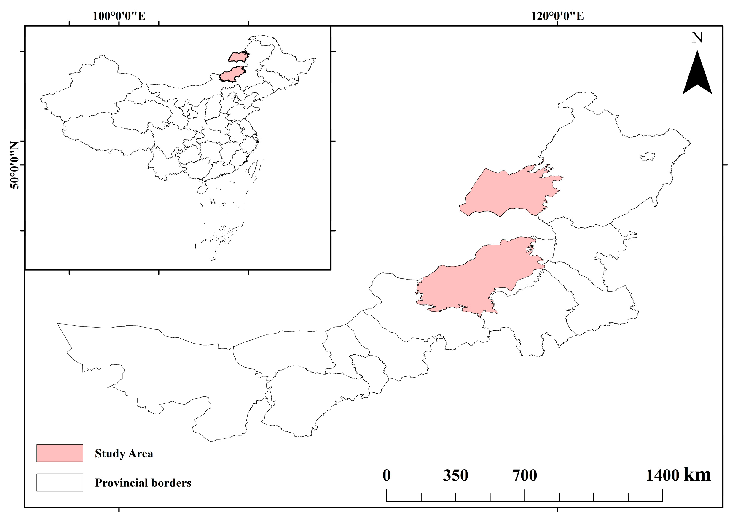
The study area is a typical grassland area in Inner Mongolia, located in the Xilingol League Prefecture near Hulunbuir City. The geographical range is 113°49′–120°26′ E, 43°08′–49°96′ N, the altitude ranges from 495–1577 m, the east–west length of the area is about 350 km, and the north–south width of the area is about 150 km, with a total grassland area of 152,521 km2 (Figure 1). The average temperature in the study area during the growing season is 17 °C, and the average precipitation in the growing season is 232 mm. The area is considered to have a northern temperate continental climate. The distribution of water resources is not balanced. There are more water resources in the eastern region, and most central and western regions are short of water resources. The cold wind in winter is strong, and both precipitation and temperature peak during the summer. The vegetation type in the study area is typical of the regional steppe, the dominant species being Stipa krylovii, S. grandis, and Leymus chinensis.
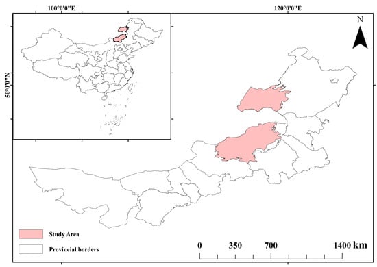
Figure 1.
Geographical location of the study area.
2.2. Research Data
The time range of this study is the growing season (May–September) from 2001 to 2022. This study used multi-source remote sensing data, including vegetation index (MOD13A2), surface temperature (MOD11A2), and evapotranspiration (MOD16A2) data from the Moderate Resolution Imaging Spectroradiometer (MODIS). The study collected precipitation data from the Climate Hazards Group InfraRed Precipitation with Station data (CHIRPS) global rainfall data set and collected soil moisture data from the Famine Early Warning Systems Network Land Data Assimilation System (FLDAS). The spatial resolution of MOD13A2 and MOD11A2 is 1000 m. The resolution of MOD16A2 is 500 m. The spatial resolution of CHIRPS data is 5566 m. The spatial resolution of FLDAS data is 11,132 m. In order to ensure all data are at the same spatial resolution and scale, all data were resampled to 1000 m resolution using the bilinear interpolation method in GEE (Google Earth Engine). Similarly, to ensure time windows were consistent, the data with different time resolutions were processed into monthly mean data by the mean value synthesis method (Table 1).

Table 1.
Description of indices obtained from sensors and orbital models.
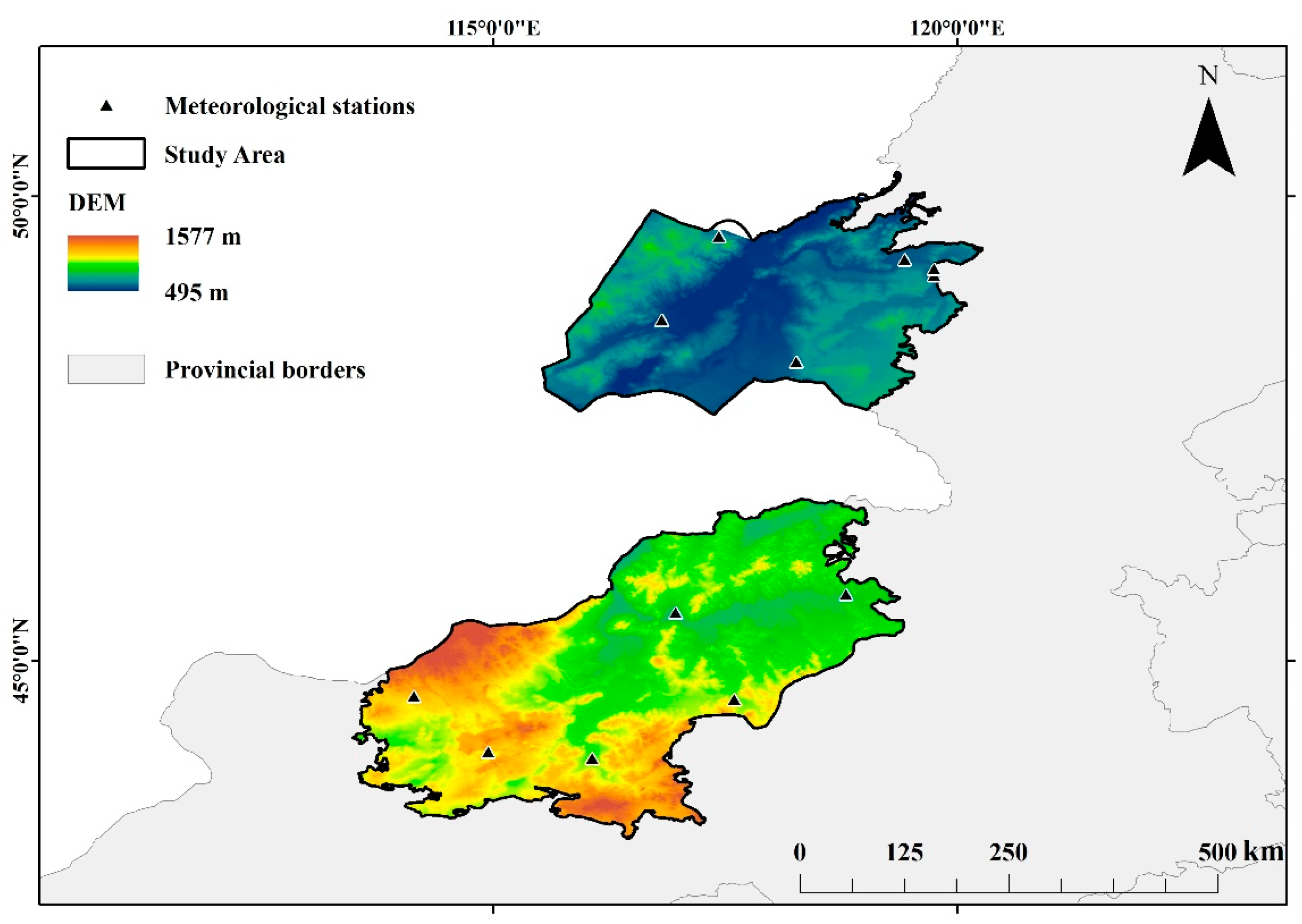
The meteorological station data used in this study are collected from stations evenly distributed across the northeast of the Inner Mongolia Autonomous Region. The monthly average temperature and monthly precipitation of 12 meteorological stations were used (Table 2). The monthly average precipitation is used to calculate SPI and SPEI, and the monthly average temperature is used to calculate SPEI. The above meteorological station data are from the Inner Mongolia Meteorological Bureau (Figure 2, Table 2).
Table 2.
The information of meteorological station data.

Figure 2.
Distribution of meteorological stations in the study area.
2.3. Characteristic Variable
The occurrence of drought is a complex process. Many factors directly or indirectly lead to drought, including increased evapotranspiration, decreased soil water content, and increased surface temperature. Furthermore, mutual feedback and time lag between vegetation and dry conditions are crucial for the construction of a drought index. Vegetation changes reflect the wet and dry conditions of the region, as well as the relationship between soil, atmosphere, and water [5,26,27,28,29]. The Normalized Difference Vegetation Index (NDVI), land surface temperature (LST), precipitation (PRE), evapotranspiration (ET), and soil moisture (SM) were selected as independent variables to construct a remote sensing drought monitoring model. The above five indicators can be used when detecting the absolute value of drought at a certain time, but they are incompetent when expressing the drought situation at a certain time in a long time series (we can identify a ‘drought’ but not its magnitude or duration). Therefore, the above five indicators are used to develop a ‘condition index’.
2.3.1. VCI
NDVI values alone are insufficient for understanding how NDVI responds to drought over a long period of time, so the VCI is used as a proxy vegetation drought parameter in this study. The VCI calculated based on NDVI can monitor the difference in productivity of an ecosystem [30] and can better reflect the impact of drought stress on vegetation. The calculation formula of VCI is as follows:
Here, NDVI, NDVImax, and NDVImin are the monthly NDVI value, the multi-year maximum value, and the multi-year minimum value of monthly NDVI in the study time range, respectively. VCI values range from 0–1. The lower the value, the worse the vegetation growth; the higher the value, the better the vegetation growth.
2.3.2. TCI
The TCI is a drought monitoring index based on LST, which is used to determine temperature-related drought phenomena [31]. When drought occurs, the decrease of soil moisture may have an indirect negative effect on soil temperature surface temperature; thus, an abnormally high surface soil temperature during the crop growing season may be considered an indicator of drought. The calculation formula of TCI is as follows:
LST, LSTmax, and LSTmin are the monthly TCI value, monthly maximum TCI value, and monthly minimum value in the study time range, respectively. The range of TCI is 0–1, and TCI is close to or equal to 0 when drought occurs. In wet conditions, the TCI is close to 1.
2.3.3. ECI
Evapotranspiration is a valuable indicator of drought [32]. The evapotranspiration status index was used to monitor the degree of vegetation water shortage in the study area for a long time. The calculation formula is as follows:
Among them, ET, ETmax, and ETmin are the monthly ET values in the study time range, the multi-year maximum value of monthly ET, and the multi-year minimum value of monthly ET, respectively. The range of ECI is 0–1. The smaller the value of ECI, the higher the evapotranspiration in the study area, and vice versa.
2.3.4. SMCI
Soil is a vital component of terrestrial ecosystems and plays an important role in regulating the energy balance of the terrestrial water cycle. Soil moisture (SM) regulates surface–plant–atmosphere interaction process, affects climate and weather processes [33], and is an important factor affecting the energy exchange between soils, plants, and the atmosphere [34]. In agricultural systems, drought can be tracked by SM, so the SMCI is used as an indicator to characterize soil information in drought monitoring [35]. The calculation formula is as follows:
Among them, SM, SMmax, and SMmin are the monthly SM value, the multi-year maximum of monthly SM, and the multi-year minimum of monthly SM in the study time range, respectively. The range of SMCI is 0–1. The higher the soil moisture, the higher the SMCI value, and vice versa.
2.3.5. PCI
Precipitation condition index (PCI) is a drought monitoring index that can provide meteorological drought information, and vegetation drought is generally caused by meteorological drought [36]. The PCI can represent the influence of long-term precipitation (Pre) changes on drought. The calculation formula is as follows:
Among them, Pre, Premax, and Premin are the monthly precipitation values within the study time range and the multi-year maximum and minimum values of the monthly Pre, respectively. PCI ranges from 0 to 1, wherein low precipitation leads to a value nearer zero and higher periods of rainfall lead to PCI values near 1.
2.3.6. SPI3 and SPI6
The Standardized Precipitation Index (SPI) is widely used in large-scale drought monitoring [37]. The index regards the continuous time series of precipitation at a certain time scale (such as 1, 3, 6, and 12 months) as obeying a certain probability density function distribution (such as gamma distribution), then derives the corresponding cumulative probability function and then converts it into a standard normal distribution. After conversion, the SPI corresponding to a certain time scale is expressed as the x-axis value of the standard normal distribution corresponding to the cumulative probability of the sample precipitation. In simpler terms, the SPI can be thought of as an index based on the average rainfall in an area over a given timescale so that ‘drought’ may be estimated as points in time that are sufficiently different for the mean rainfall in that region. The drought grade of SPI is shown in Table 3:
Table 3.
SPI drought level.
2.3.7. SPEI
The Standardized Precipitation Evapotranspiration Index (SPEI) is a standardized drought index that comprehensively considers precipitation and evapotranspiration [38]. The absolute value of SPEI reflects the degree of drought or wetness. The principle of this index is to assume that the difference between precipitation and evapotranspiration obeys the Log-logistic probability distribution and standardizes it to obtain the following equation:
In this equation, = 2.515517, = 0.802853, = 0.010328, = 1.432788, = 0.189269, and = 0.001308. The classification of the SPEI drought grade is shown in Table 4.
Table 4.
SPEI drought level.
2.4. Model
2.4.1. Back Propagation
The BP (Back Propagation) neural network framework was first proposed by a group of scientists led by Rumelhart and McClelland in 1986. It is a multi-layer feedforward network trained by error backpropagation and is one of the most widely used neural network models [39]. Liu applied the BP neural network to agricultural drought monitoring in 2020 and achieved good monitoring results [40]. A number of studies have shown that BP has a good fitting effect in the construction of drought monitoring index [41,42]. Its basic algorithm is based on the gradient descent method, using gradient search technology so that the error and mean square error of the predicted value and the actual output value of the training network are the lowest. The topology of a conventional BP neural network model includes an input layer, a hidden layer, and an output layer.
Using MATLAB R2020b, we can train a BP neural network using the newff function to construct a comprehensive drought monitoring model. In this model, ‘epochs’ represents the maximum number of training sessions, ‘goal’ indicates the accuracy required for training, and ‘lr’ represents the learning rate of the model. The model parameters are shown in Table 5:
Table 5.
BP neural network parameters.
2.4.2. Support Vector Machines
Support vector machines (SVMs) are novel data mining tools based on statistical learning theory. SVMs have dealt well with regression problems (time series analysis), pattern recognition (classification and discriminant analysis), and many other problems. SVM approaches have been used for binary classification problems, and support vector regression (SVR) is an important application branch of support vector machine. SVR and SVMs are both derived from the concept of support vector machines, but they are tailored for several types of predictive modeling problems. SVM aims to find the optimal hyperplane that separates different classes in feature space. The objective is to maximize the margin between the nearest points of the classes, which are called support vectors. SVMs can handle both binary and multi-class classification problems. SVR, on the other hand, is used for regression tasks. Instead of trying to maximize the margin between two classes, an SVR attempts to fit the best hyperplane that can predict continuous values within a certain margin of tolerance (epsilon). The goal is to minimize the error within this epsilon margin while also trying to keep the model as flat as possible (minimizing the norm of the coefficients) to prevent overfitting. While an SVM focuses on maximizing the margin between classes for classification tasks, an SVR focuses on fitting a hyperplane that can predict continuous outcomes with a certain tolerance of errors for regression tasks.
Many studies have applied SVM to the construction of drought monitoring index, showing more obvious regional characteristics in terms of correlation with other meteorological stations [6,43,44,45]. This study uses SVMcgForRegress and Svmtrain functions in the MATLAB LIBSVM algorithm package to train and construct a comprehensive drought monitoring model. The penalty coefficient and gamma coefficient are calculated by cross-parameter verification. The specific training parameters are shown in Table 6:
Table 6.
SVR parameter settings.
2.4.3. Random Forest
Random forest model frameworks are commonly used approaches to machine learning simulations. The basic unit of the Random “forest” is the decision tree, and multiple decision trees are integrated by using the idea of ensemble learning. Thus, the ‘Forest’ refers to a network of multiple decision trees. Randomness is reflected in two aspects: the randomness of samples and the randomness of features. For the regression problem, the final regression result can be obtained by averaging the output of each decision tree [46]. The advantage of the random forest model is that it is useful for simulating many features with high dimensions, in that high accuracy results can be obtained without dimension reduction. Further, RF model approaches are less sensitive to outliers and missing values, making RF a useful tool for processing data with missing values. However, when the training data noise is large, the model is also prone to overfitting.
Yue et al. used RF, SVM and BP to monitor drought in the North China Plain and found that RF has high accuracy in drought monitoring [41]. A number of studies have shown that RF has a good fitting effect in the construction of drought monitoring index [44,47,48]. In this study, the TreeBagger function in MATLAB was used to construct a random forest model, and the optimal number of leaves and decision trees was screened through multiple cycles. Model parameters implication and settings are shown in Table 7 and Table 8, respectively:
Table 7.
Random Forest network parameter implication.
Table 8.
Random forest network parameter settings.
2.4.4. Convolutional Neural Network
Deep learning is a new evolution of traditional machine learning research, designed to enable the computer to learn the inherent characteristics of a dataset from a large pool of sample data and classify and predict the newly received samples. Convolutional neural networks (CNN) are one of the more common deep learning frameworks. CNNs utilize layers of convolutional filters to automatically detect and learn hierarchical patterns and features from the input data. Through a combination of convolutional layers, pooling layers, and fully connected layers, CNNs effectively capture spatial and temporal dependencies. This makes them particularly suited for tasks in image and video recognition, image classification, and any application requiring the analysis of visual input.
Hao et al. used CNN to monitor the meteorological and hydrological drought in the Huaihe River Basin and achieved good monitoring results [49]. Several studies have shown that CNN has a good fitting effect in the construction of drought monitoring index [47,50]. The model uses a convolution kernel, a normalization layer, a modified linear unit layer (ReLU) and a fully connected layer. The model parameters implication and settings are shown in Table 9 and Table 10, respectively:
Table 9.
CNN model parameter implication.
Table 10.
CNN model parameters.
2.5. Process of Model Construction
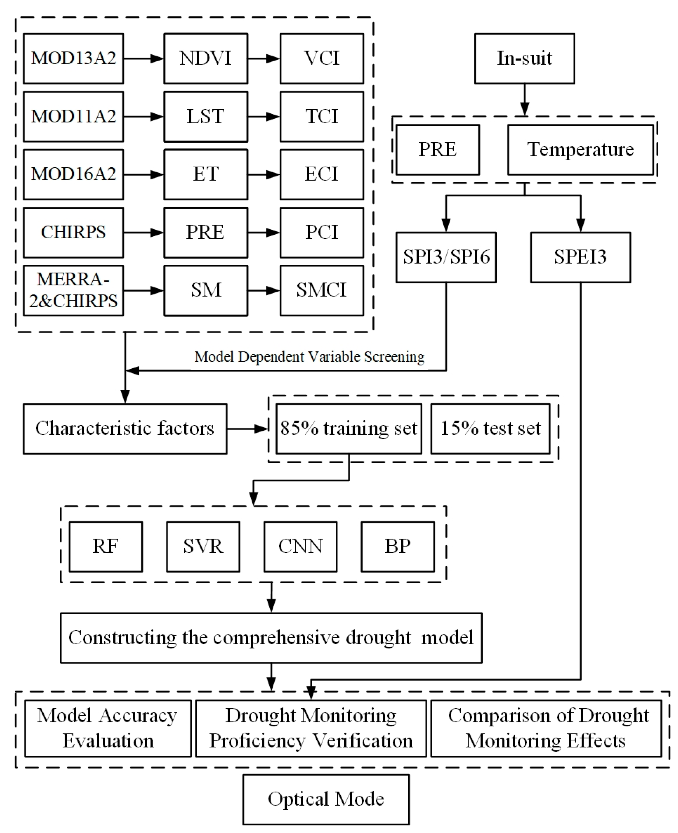
To comprehensively consider the combined effects of precipitation, vegetation, and soil on drought in the process of constructing the drought index, the five independent variables (VCI, TCI, ECI, SMCI, and PCI) and the dependent variable SPI3 were selected above. Based on the random forest model (RF), convolutional neural network model (CNN), support vector regression (SVR), and BP neural network, a comprehensive drought monitoring model with SPI = f (VCI, TCI, ECI, SMCI, and PCI) was constructed and named (CDMI). The coefficient of determination (R2) and root mean square error (RMSE) were used to evaluate the fitting accuracy of the comprehensive drought monitoring model. The data for the same month from 2001 to 2022 were divided into five groups, and the data for 22 months in each group were calculated. 85% of the total pixel number was set as the training set, and 15% was set as the test set for model training and validation. The flowchart for model construction is presented in Figure 3.
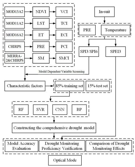
Figure 3.
Flowchart of the methods used in this study.
3. Results
3.1. Model Dependent Variable Screening
In this study, five environmental factors (VCI, TCI, ECI, SMCI, and PCI) and standardized precipitation index (SPI3/SPI6), which characterize drought from climate, vegetation, and hydrological data sources, were selected for annual and monthly Pearson correlation analysis to study the response of different environmental factors to drought in the study area.
According to the correlation analysis and comparison, the correlation between environmental factors and SPI3 is higher than that of SPI6, and all five factors have passed the 0.01 significance test (Table 11). Except for evapotranspiration, environmental factors were positively correlated with SPI. PCI and SMCI were highly correlated with SPI, and the correlation between SPI3 and PCI was 0.81. The correlation between ECI and SPI3 was the lowest, only −0.59; the correlation between other indicators and SPI3 was between 0.6–0.8.
Table 11.
Pearson correlation coefficients between the five drought indicators and SPI at different month scales used in this study.
The response of each factor to drought was different in different growing seasons. Correlation analysis between each factor and SPI was conducted on the monthly data, and all the results passed the 0.01 significance test (Table 12). In the growing season (May-September), the correlation between SPI3 and SPI6 was small, but SPI3 was higher than SPI6, which was consistent with the comparison results at the annual scale. Among the five environmental factors, the correlation between precipitation and SPI3 was the highest, and the correlation coefficient ranged from 0.37 to 0.66. Across time, the correlation between May and July was higher than 0.55, and the correlation between August and September was lower, only reaching 0.4. The correlation between vegetation and land surface temperature has the same change trend, the lowest in May, which is 0.2–0.3, and the highest in June–September, when the correlation coefficient reaches 0.45–0.65. The correlation between land surface temperature and SPI is slightly higher than that of vegetation indices and SPI. There was a high correlation between soil moisture and SPI3, except that the correlation coefficient was only 0.38 in September; in the other months, it was more than 0.45. The correlation between evapotranspiration and SPI3 was the lowest, and the correlation coefficient was between −0.2 and −0.3.
Table 12.
Monthly correlation analysis between drought indicators and SPI.
According to the annual and monthly correlation analysis of SPI3 and SPI6, it can be concluded that the correlation coefficient between SPI3 and environmental factors is higher than that of SPI6 (p < 0.01). The correlation between precipitation and SPI3 was the highest, with a significant positive correlation. Soil moisture, surface temperature and vegetation were well correlated with SPI3. The correlation between evapotranspiration and SPI3 was low and negatively correlated. These results suggest that precipitation has the greatest impact on drought in the study area, followed by soil moisture, surface temperature, vegetation growth, and evapotranspiration. Therefore, in the following machine learning research, SPI3 is selected as the dependent variable of the machine learning model, and VCI, TCI, SMCI, ECI, and PCI are selected as the independent variables to construct the machine learning model.
3.2. Model Accuracy Evaluation Results
The accuracy evaluation results of the test set of the comprehensive drought monitoring index (CDMI) are shown in Table 13 and Table 14 and Figure 4. R2 was used to verify the correlation between the comprehensive drought monitoring index constructed by the four machine learning models and the measured SPI3.
Table 13.
Comparison of four model test sets for R2.
Table 14.
Comparison of four model test sets for RMSE.
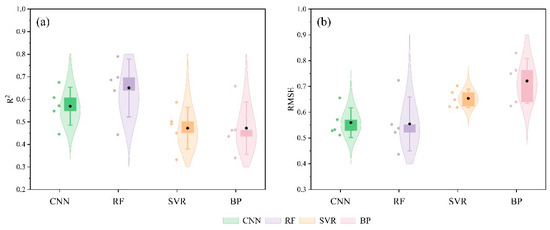
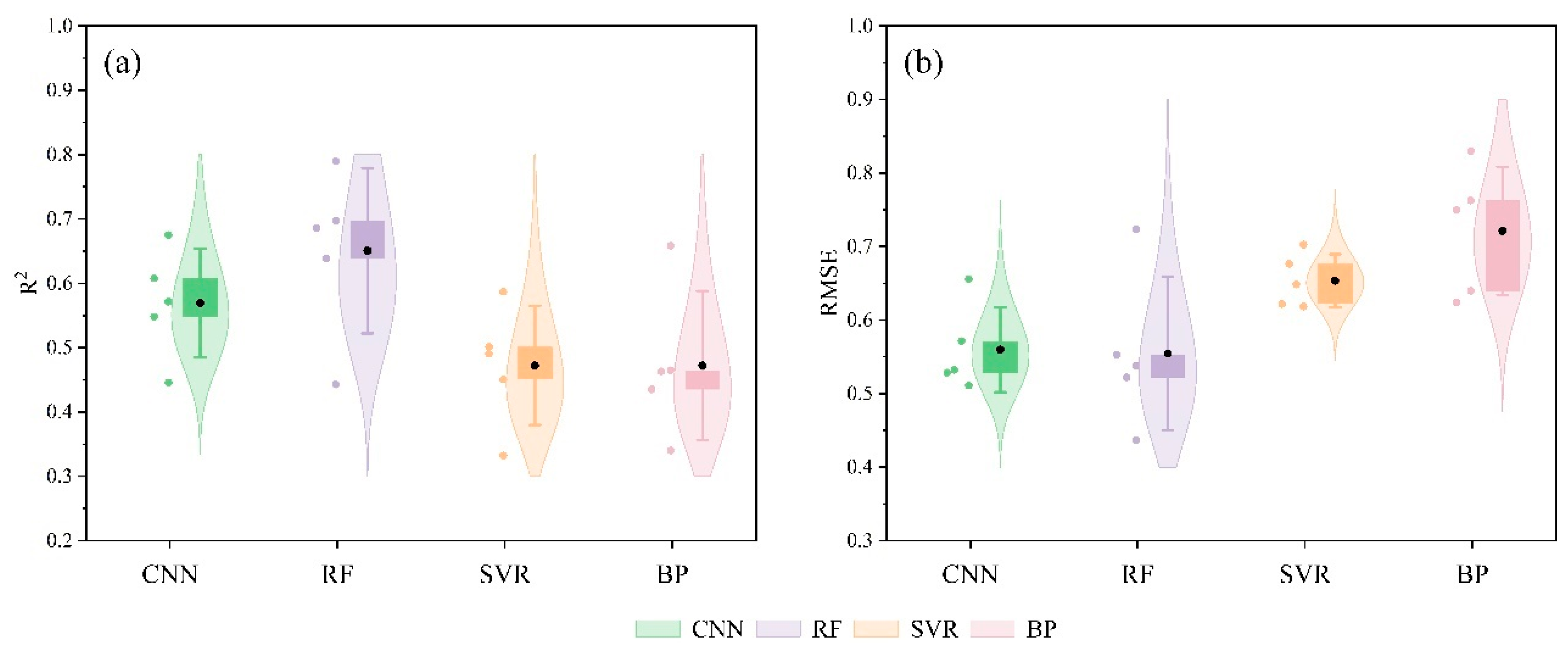
Figure 4.
Model accuracy of the testing set. (a) R2; (b) RMSE.
We observed that the R2 range of the comprehensive drought monitoring index based on the RF model ranged from 0.44–0.79, the R2 range of the CNN model ranged from 0.45–0.68, and the R2 range of the SVR model ranged from 0.33–0.59 (Table 13). The R2 range of the BP neural network model ranged from 0.31–0.60. Further, the comprehensive drought monitoring index has monthly scale differences. In all models, the model was the least accurate in September and most accurate in July. According to the comparison of R2 violin plots, it can be found that among the four machine learning models, the average R2 of the comprehensive drought monitoring index based on the random forest model is the highest, R2 > 0.60; the CNN model is second only to RF, 0.60 > R2 > 0.55; the accuracy of SVR is close to that of BP neural network, and the R2 range is between 0.4 and 0.5. The accuracy of the four models could be represented as RF > CNN > SVR ≈ BP.
RMSE was used to analyze the deviation between the predicted value and the measured value of the four models. We observed that the RMSE range of RF is 0.44–0.72, the RMSE range of CNN is 0.51–0.66, and the model deviation is low (Table 14). The RMSE range of SVR is 0.62–0.70, the RMSE range of BP is 0.61–0.80, and the model deviation is high (Table 14). The comparison between different months of the same model shows that there are also differences in the monthly scale of different models. The monthly scale difference of RMSE of the four models was compared. The results showed that the deviation degree of RF and CNN in September was the highest, and the deviation value of the model from May to August was significantly lower than that in September. The two models may be more sensitive to changes in vegetation or climatic conditions at the end of the growing season. However, a non-significant monthly scale difference was found between BP and SVR, indicating that these two models are insensitive to this change (Table 14). The average RMSE of RF and CNN is 0.5–0.6, and the deviation degree of the two models is the same. The average RMSE of SVR is between 0.6–0.7, and the average RMSE of BP is between 0.7–0.8, which are higher than RF and CNN. The comparison shows that the BP approach is arguably the least accurate, with the highest amount of deviation and the lowest amount of model fit (represented by the lower R2). The degree of deviation between the four models could be represented as RF > CNN > SVR > BP. In summary, the drought monitoring index constructed by the random forest model was the most accurate and has the best fit. The difference in accuracy between the random forest model and the CNN model is small, but the accuracy of the other two models is significantly lower than that of RF.
3.3. Drought Monitoring Proficiency Verification
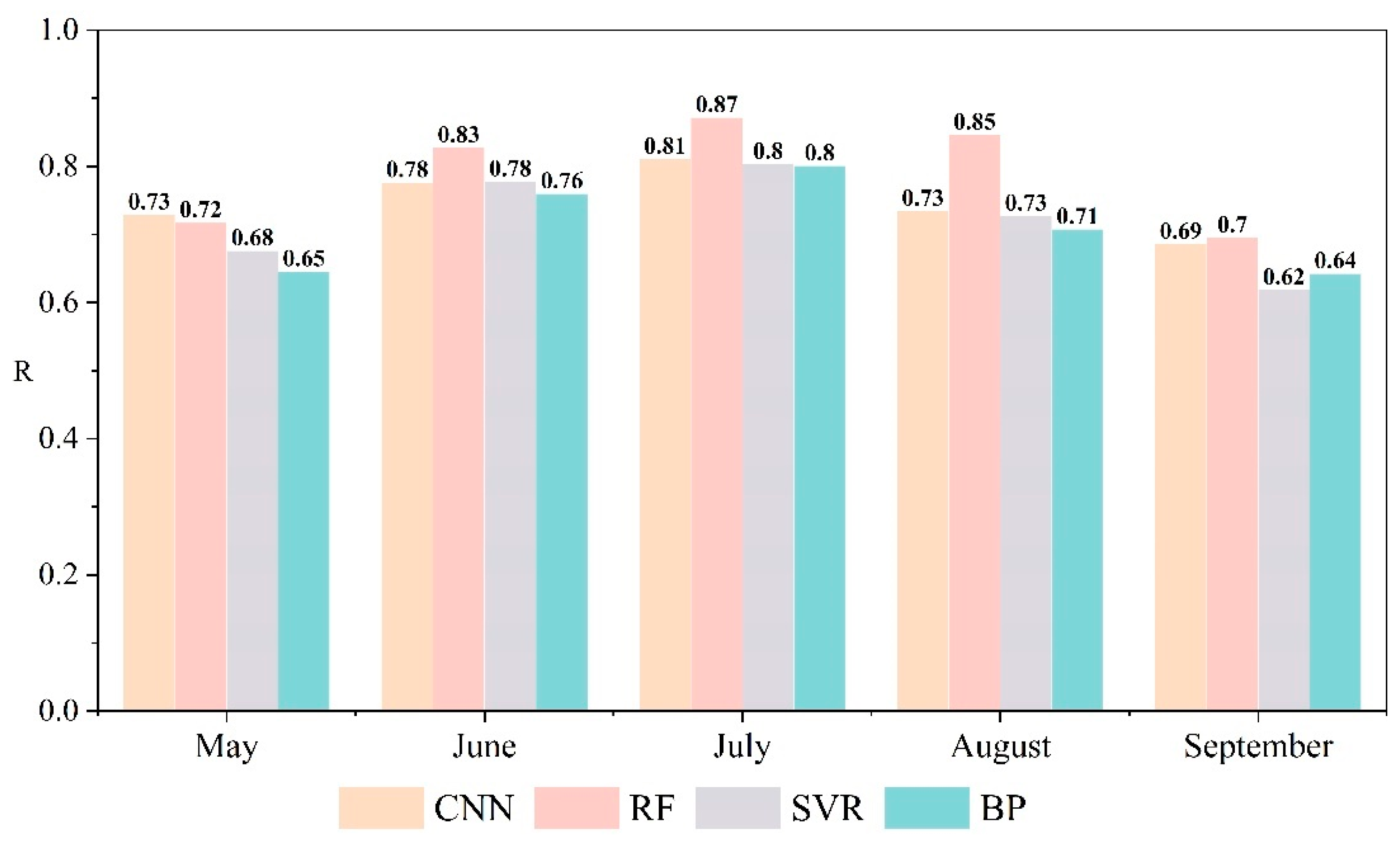
Relevant studies have shown that in arid and semi-arid areas, vegetation growth and ecosystem health status depend directly on atmospheric precipitation [11,51]. Therefore, this study uses SPEI to test the drought monitoring ability of machine learning models. The SPEI index is calculated using evapotranspiration and precipitation data. The index combines the sensitivity of drought to changes in evaporation demand (caused by temperature fluctuations and trends) with the simplicity of calculation and the multi-temporal characteristics of SPI. It is more suitable for large-scale and long-term regional drought monitoring [38,52,53]. The short-time series SPEI1 and SPEI3 are generally used to monitor meteorological drought, while the long-time series SPEI6 and SPEI12 are used to detect agricultural drought and hydrological drought [54]. Pei’s research has shown that SPEI3 is more suitable for drought monitoring in Inner Mongolia grassland [52], and it can be consistent with SPI3 on the time scale, so SPEI3 is selected in this study. It is a commonly used meteorological drought monitoring indicator. In this study, 12 meteorological stations were used to calculate the SPEI3 of the long-term series (2001–2022) to compare and verify the drought monitoring capabilities of the four machine-learning models. Pearson correlation analysis was performed between the prediction results of the four models and SPEI3. The results are shown in Figure 5.
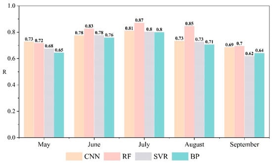
Figure 5.
Correlation between the four models and SPEI3 in different months (p < 0.01).
According to the analysis results, the correlation between the CNN model and SPEI in May is the highest, R = 0.73, followed by the correlation between RF and SPEI, R = 0.72, and then finally, the other two models wherein R < 0.7, suggesting low correlation. Among all models, the correlation between RF and SPEI3 in June–September is the highest. The Pearson’s correlation, R, in June–August for the RF model is greater than 0.8, and the other three models are significantly different from RF. In September, the correlation of all four models to SPEI was low, though RF was slightly higher than CNN, and both were significantly higher than the other two models. Except for May and September, the correlation coefficients in other months were higher than 0.8, and the above results all passed the 0.01 significance test. The results show that the comprehensive drought monitoring index based on RF can effectively improve the ability of models to simulate drought indices on a typical grassland area in Inner Mongolia [41].
3.4. Comparison of Drought Monitoring Effects
After generating our drought data, we wanted to represent the geographical variation across our landscape in an easily interpretable way. Thus, we generated a regional map divided into drought zones over a gradient scale with equal interval steps from most droughted to least.
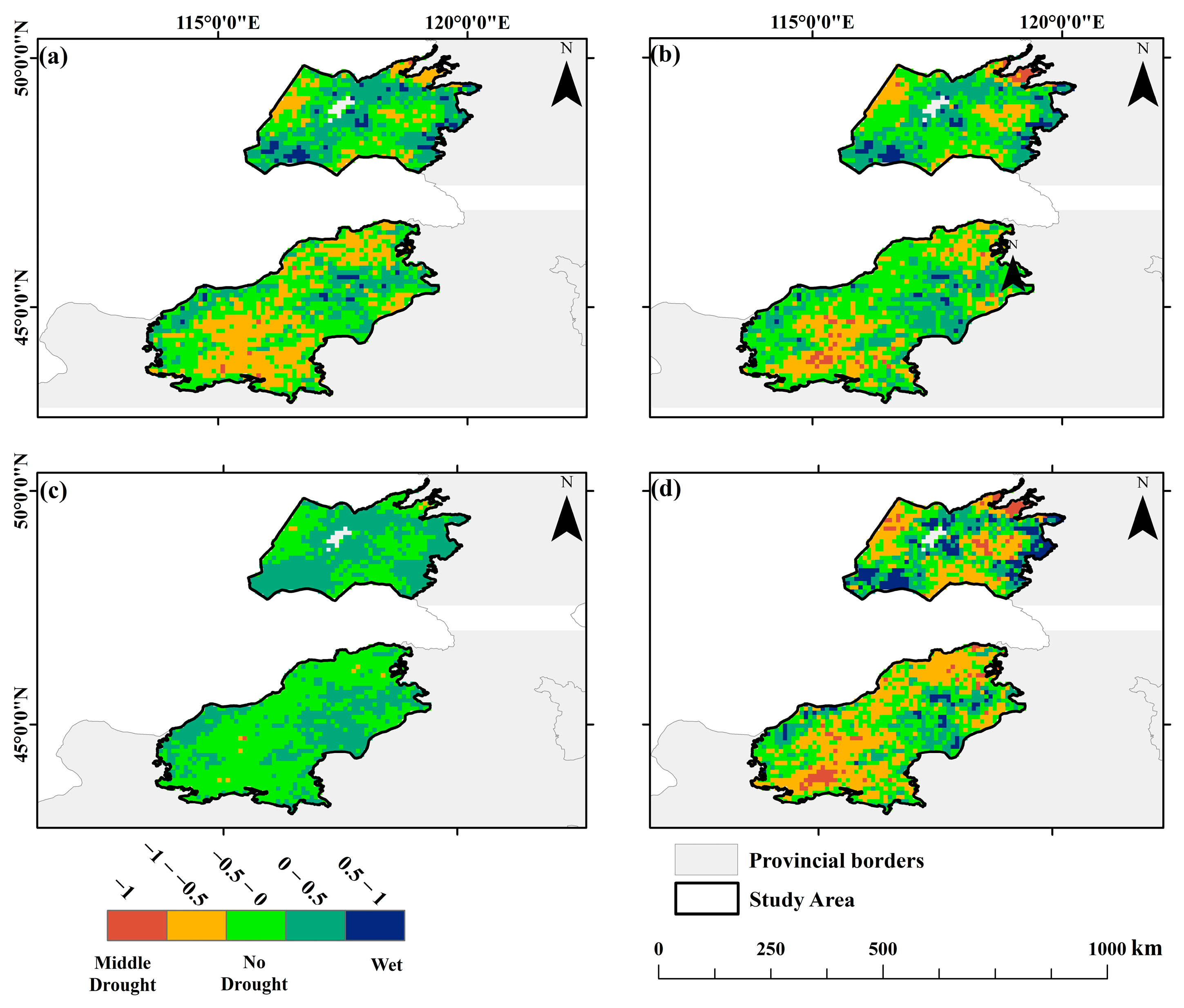
Using data from July 2019, this study takes meteorological stations as sampling points, obtains the pixel values of remote sensing data at the corresponding positions as the initial data to train the machine learning model, fits the model to the observed remote sensing data pixel by pixel, and draws the results into a spatial distribution map (Figure 6).
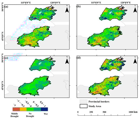
Figure 6.
Comparison of four machine learning models. (a) RF, (b) CNN, (c) SVR, and (d) BP. Colors represent drought degree: the redder the color, the stronger the level of drought.
Comparing the spatial distribution maps drawn by the four machine learning models, the fit was best in the RF model, perhaps because RF frameworks minimize the influence of extremely high and extremely low values, smoothing the rough gradient of the interpolation data. The BP approach, on the other hand, allows abnormally high or low values at the boundary of the study area and the area of gradient change, which affects the accuracy of the model’s prediction of drought gradient. Compared with other models, the BP framework has more pronounced spatial heterogeneity. This phenomenon also exists in CNN. Through the above comparison, the RF approach is the most accurate, followed by CNN. BP and SVR have obvious defects.
4. Discussion
4.1. Analysis of Drought Factors
Drought is one of the most common and frequent natural disasters in the world, and it is very difficult to accurately monitor drought [55]. The occurrence of drought is related to the complex interaction of precipitation, temperature, evapotranspiration, and vegetation. While drought monitoring indices constructed using only one of these data streams can estimate the influence of that data on drought, the complex interactions among environmental factors such as different climate types and geographical landforms may affect the ability to truly monitor all drought effects. For example, NDVI is used for drought monitoring in grassland areas with obvious seasonal differences in precipitation, but the use of NDVI in agriculturally developed areas will affect the judgment of drought due to differences in planting structure. At present, the Inner Mongolia region uses SPI, SPEI and other drought monitoring indexes based on precipitation or TVDI, NDVI and other drought monitoring indexes based on vegetation elements to monitor drought. However, the Inner Mongolia Autonomous Region is not a traditionally modeled ecosystem (e.g., a temperate or tropical lowland forest). The region is a narrow band of high-altitude desert grassland and forest that has complex vegetation heterogeneity and a good deal of topographical variation. At present, we lack a multivariate comprehensive drought monitoring index that can accurately represent this landscape [56].
In this study, five drought factors were selected as the independent variables of the model input. These factors have the same contribution rate by default before entering the model, but their contribution rates are different when the model outputs the final simulation results. In order to study the influence of each drought factor on the simulation results, we calculated the contribution ratio of different months and different drought factors (Table 15). The results showed that the contribution rate of different drought factors varied greatly in different months. From May to June, the contribution rate of PCI was highest, and it was affected by the natural conditions of Inner Mongolia. May and June are the early growing seasons of typical grasslands, when the vegetation coverage is low, and precipitation and bare surface greatly influence drought monitoring. The contribution rate of LST and VCI was higher from July to September, and the sum of them was more than 50%. This indicated that vegetation growth and land surface temperature play an important role in the formation and development of drought during this period. This is mainly because the transpiration of healthy vegetation reduces the surface temperature and reduces the loss of soil moisture. When vegetation growth is weak or the surface temperature is high, soil water loss occurs, causing regional drought. Therefore, drought is more likely to occur in the early growing season (May–June), when the surface is bare, and when precipitation decreases, drought occurs in the region. The surface vegetation coverage in the middle and late growing season (July–September) is high. When precipitation decreases, the surface plants’ water content and soil moisture can regulate drought [19].
Table 15.
Percentage contribution of drought factors.
4.2. Comparison of Drought Monitoring Capabilities of Models
With the continuous development of drought monitoring technology research, the study of drought monitoring index constructed by single factor is gradually changing to the study of multi-factor drought monitoring index. This study comprehensively considers multiple factors affecting drought, selects four machine learning models (BP, SVR, RF, and CNN), constructs a comprehensive drought monitoring index, and compares the four models through methods such as accuracy evaluation and drought capacity verification.
Compared with the results of other studies, we found that RF had a good fitting effect in different regions, different climate types, and different drought types. Compared with the Inner Mongolia grassland area, the climate of Shaanxi Province has higher average temperatures, smaller temperature differences, and higher air humidity during the growing season. The results of drought monitoring in Shaanxi Province by Han et al. showed that RF constructed the drought monitoring index had a good fitting effect, which had a high correlation with SPI (R = 0.5, p < 0.01) [57]. The major land use types in the North China Plain were cultivated land rather than grassland, and there were differences in hydrothermal conditions between these two places. The results of Yue et al.’s study found that RF was suitable for drought monitoring in this area (R2 = 0.789, RMSE = 0.454, and MAE = 0.348). The fitting accuracy of RF was better than BP and SVR, which is consistent with the results of this study [41]. Iran is located in a semi-arid area, and the land use types are mainly desert and cultivated land. Heidarizadi et al. also found that RF had good applicability for SPI prediction (R2 = 0.88) [48]. The above results showed that RF could carry out drought monitoring and achieved good results in different land use types, different climatic conditions and different regions.
We found the RF framework to be the best for generating drought monitoring data for Inner Mongolia. RF model approaches are ensemble learning tools based on generating decisions through a ‘random’ ‘forest’ of decision trees. Most importantly, RF models can ‘smooth’ large data sets with substantial numerical differences due to outliers, improving the generation of regional scale data from a limited number of sources. Further, RF is computationally cheap—the parallel operation of the decision tree means the model can run quickly and efficiently without computational strain. The SVR model is a linear classifier that excels in handling high-dimensional data due to its use of kernel functions for optimal hyperplane identification. However, its performance diminishes with large datasets as it requires high-order matrix computations, consuming substantial time and computer memory. The BP framework is similarly constrained—it takes a long time to train a BP model, and the overall accuracy is limited. Consistent with this result, Cheng et al. found that random forest outperforms SVR in drought monitoring, aligning with findings that highlight the limitations of SVR and BP neural networks with large data volumes [44]. Meanwhile, BP neural networks demand extensive training iterations without clear guidelines on network structure.
In this paper, we found that CNN was the ‘next-best’ choice after RF for generating our drought index. This is consistent with what others have seen—Prodhan found that the overall performance of deep learning is comparable to that of random forest, and its multi-layer method can find the best output in the case of high-dimensional data features [58]. However, the pooling layer of the CNN model will lead to the loss of some key features during training, which may be one of the reasons why the accuracy of the training model is lower than that of the random forest model. CNNs, as deep learning exemplars, offer high accuracy and efficiency in processing large datasets, though they may lose some features due to pooling layers, slightly lowering accuracy compared to random forest. Overall, deep learning demonstrates potential in multivariate drought monitoring, as shown by Shen et al. with their DFNN model in Henan Province, underscoring the promising application of deep learning in comprehensive monitoring models [19].
4.3. Advantages and Limitations of Drought Monitoring Model
According to an assessment of the model’s monitoring capabilities and a comparison with conventional meteorological monitoring techniques, the comprehensive drought monitoring index developed in this work offers the following benefits: (1) The comprehensive drought monitoring index constructed in this study considers multiple environmental factors that affect drought, including vegetation growth status, surface temperature, precipitation, soil moisture, evapotranspiration, etc. Therefore, the index has the ability to monitor multiple drought types. (2) The traditional meteorological interpolation method obtains high-precision spatial monitoring results by laying many dense meteorological stations. The model constructed in this study not only uses free remote sensing data and a small amount of meteorological station data but also obtains high-resolution and high-precision monitoring results. In addition, the method proposed in this study reduces the cost of drought monitoring and provides a technological method for achieving regional-scale drought monitoring.
Based on remote sensing data and meteorological station data, this paper uses machine learning models to construct a comprehensive drought monitoring index suitable for typical grassland areas in Inner Mongolia, but there are still many deficiencies in this research. (1) In this study, data from the 2001–2022 growing season (May to September) were used, and drought conditions in autumn and winter were not analyzed. In addition, the data period used in this study is short, and the use of monthly data calculation also affects the model accuracy. In the future, we will use longer time series and higher temporal resolution data to improve the monitoring accuracy of the model. (2) Limited by the number of meteorological stations, this study uses limited ground observation data. Increasing the distribution density of meteorological stations can improve the model’s accuracy and reduce the error when drawing the spatial distribution map. (3) When constructing the comprehensive drought monitoring index, the environmental factors considered are not rich enough. The terrain, slope, land cover, types of human activities and other factors also impact drought. More parameters can be added in the future to improve the drought-monitoring ability of the model [19]. (4) The machine learning model used in this study is relatively basic. With the development of machine learning and deep learning, more advanced and more advanced models can be selected for further research in the future.
5. Conclusions
Drought is complex. The concept of ‘drought’ may be reflected by a number of variables, including precipitation (i.e., drought is decreased precipitation), vegetation (drought is the desiccation of vegetation and reduced growth/photosynthetic capacity induced by water limitation), and soil (drought is the reduction of soil moisture). Therefore, more and more studies seek a comprehensive index based on multi-parameter construction rather than a single index (such as NDVI, LST, etc.) when evaluating drought conditions. In this paper, the typical grassland area of Inner Mongolia is taken as the research area, and the multi-source remote sensing data such as precipitation, vegetation and soil moisture are combined with meteorological stations. Four machine learning models (RF, CNN, BP, and SVR) are selected to train the comprehensive drought monitoring index suitable for the study area’s growth season (May–September) from 2001 to 2022. The accuracy evaluation, drought monitoring ability detection and spatial pattern analysis of the four models were carried out to screen out the most suitable machine learning model for constructing drought monitoring index in the study area. The main conclusions are as follows:
- VCI, TCI, SMCI, ECI, and PCI were used as model-independent variables, and SPI was used as a model-dependent variable to train the machine learning model. The model fitting accuracy showed that the RF model had the highest fitting accuracy, wherein the R2 range of the test set was 0.44–0.79, and the RMSE range was 0.44–0.72. The CNN model is second; the R2 ranged from 0.45–0.68, and the RMSE ranged from 0.51–0.66; the fitting accuracy of SVR and BP was low. The R2 range of the test set is between 0.3 and 0.6, and the RMSE range is between 0.60 and 0.80. The accuracy of the four models could be described as RF > CNN > SVR ≈ BP, and the random forest model is superior to other models.
- The drought monitoring ability of the four models was evaluated, and the correlation between the model fitting value and the SPEI3 calculated based on observed data was analyzed. The results show that the correlation coefficient of CNN is slightly higher than that of RF in May (CNN = 0.79, RF = 0.78), though the correlation coefficient of RF from June to September is higher than that of the other three models. The results also show that in meteorological drought monitoring, the comprehensive drought monitoring index based on RF has a higher drought monitoring ability and can basically achieve the same effect as SPEI3.
- The four comprehensive drought monitoring indexes were drawn into a spatial distribution map to compare the regional monitoring capabilities of the four models. In the division of drought gradient, RF is the most accurate, followed by CNN. RF is more accurate in describing the boundary of the study area and the area of gradient change, while BP and SVR have a large error. Using machine learning combined with multivariate remote sensing data to construct a comprehensive drought monitoring index has high accuracy on the spatial scale.
- This study can scientifically and effectively monitor and prevent drought in Inner Mongolia’s grassland area and provide theoretical reference and technical support for drought monitoring and prevention in arid and semi-arid areas.
Author Contributions
Conceptualization, Y.W. (Yuchi Wang); Methodology, Y.W. (Yuchi Wang); Software, C.J.; Validation, Y.W. (Yuchi Wang) and J.C.; Formal analysis, Y.W. (Yuchi Wang); Investigation, Z.L.; Resources, Y.W. (Yongli Wang); Writing—original draft, Y.W. (Yuchi Wang); Writing—review & editing, B.M. and C.L. All authors have read and agreed to the published version of the manuscript.
Funding
This research was funded by The Science and Technology program of the Inner Mongolia Autonomous Region of China (2021GG0386) and Department of Science and Technology of Inner Mongolia Autonomous Region (2020GG0092).
Data Availability Statement
The original contributions presented in the study are included in the article, further inquiries can be directed to the corresponding author.
Conflicts of Interest
The authors declare no conflict of interest.
References
- Wilhite, D.; Glantz, M. Understanding the drought phenomenon: The role of definitions. Water Int. 1985, 10, 111–120. [Google Scholar] [CrossRef]
- Dai, A. Drought under global warming: A review. WIREs Clim. Change 2011, 2, 45–65. [Google Scholar] [CrossRef]
- Dai, A.; Trenberth, K.E.; Qian, T. A Global Dataset of Palmer Drought Severity Index for 1870–2002: Relationship with Soil Moisture and Effects of Surface Warming. J. Hydrometeorol. 2004, 5, 1117–1130. [Google Scholar] [CrossRef]
- Faiz, M.A.; Zhang, Y.; Tian, X.; Tian, J.; Zhang, X.; Ma, N.; Aryal, S. Drought index revisited to assess its response to vegetation in different agro-climatic zones. J. Hydrol. 2022, 614, 128543. [Google Scholar] [CrossRef]
- Méndez, C.; Simpson, N. Climate Change 2023: Synthesis Report (Full Volume) Contribution of Working Groups I, II and III to the Sixth Assessment Report of the Intergovernmental Panel on Climate Change; Intergovernmental Panel on Climate Change: Geneva, Switzerland, 2023. [Google Scholar] [CrossRef]
- Zhao, Y.; Zhang, J.-H.; Yun, B.; Zhang, S.; Yang, S.; Henchiri, M.; Seka, A.; Nanzad, L. Drought Monitoring and Performance Evaluation Based on Machine Learning Fusion of Multi-Source Remote Sensing Drought Factors. Remote Sens. 2022, 14, 6398. [Google Scholar] [CrossRef]
- Lesk, C.; Rowhani, P.; Ramankutty, N. Influence of extreme weather disasters on global crop production. Nature 2016, 529, 84–87. [Google Scholar] [CrossRef] [PubMed]
- Zhang, L.; Jiao, W.; Zhang, H.; Huang, C.; Tong, Q. Studying drought phenomena in the Continental United States in 2011 and 2012 using various drought indices. Remote Sens. Environ. 2017, 190, 96–106. [Google Scholar] [CrossRef]
- Liu, S.; Kang, W.; Wang, T. Drought variability in Inner Mongolia of northern China during 1960–2013 based on standardized precipitation evapotranspiration index. Environ. Earth Sci. 2016, 75, 145. [Google Scholar] [CrossRef]
- Huang, J.; Sun, S.; Xue, Y.; Zhang, J. Changing characteristics of precipitation during 1960–2012 in Inner Mongolia, northern China. Meteorol. Atmos. Phys. 2014, 127, 257–271. [Google Scholar] [CrossRef]
- Ji, B.; Qin, Y.; Zhang, T.; Zhou, X.; Yi, G.; Zhang, M.; Li, M. Analyzing Driving Factors of Drought in Growing Season in the Inner Mongolia Based on Geodetector and GWR Models. Remote Sens. 2022, 14, 6007. [Google Scholar] [CrossRef]
- Nakicenovic, N.; Swart, R. Special Report on Emissions Scenarios (SRES)—A Special Report of Working Group III of the Intergovernmental Panel on Climate Change; Intergovernmental Panel on Climate Change: Geneva, Switzerland, 2000; Volume 559. [Google Scholar]
- Svoboda, M.; LeComte, D.; Hayes, M.J.; Heim, R.; Gleason, K.L.; Angel, J.R.; Rippey, B.; Tinker, R.; Palecki, M.A.; Stooksbury, D.E.; et al. The Drought Monitor. Bull. Am. Meteorol. Soc. 2002, 83, 1181–1190. [Google Scholar] [CrossRef]
- Portela, M.M.; dos Santos, J.F.; Silva, A.T.; Benitez, J.B.; Frank, C.; Reichert, J.M. Drought analysis in southern Paraguay, Brazil and northern Argentina: Regionalization, occurrence rate and rainfall thresholds. Hydrol. Res. 2014, 46, 792–810. [Google Scholar] [CrossRef]
- Ibrahim, A.; Harrison, M.T.; Meinke, H.; Zhou, M. Examining the yield potential of barley near-isogenic lines using a genotype by environment by management analysis. Eur. J. Agron. 2019, 105, 41–51. [Google Scholar] [CrossRef]
- Yin, J.; Zhan, X.; Hain, C.R.; Liu, J.; Anderson, M.C. A Method for Objectively Integrating Soil Moisture Satellite Observations and Model Simulations toward a Blended Drought Index. Water Resour. Res. 2018, 54, 6772–6791. [Google Scholar] [CrossRef]
- Zargar, A.; Sadiq, R.; Naser, B. A review of drought indices. Environ. Rev. 2011, 19, 333–349. [Google Scholar] [CrossRef]
- Prodhan, F.A.; Zhang, J.; Hasan, S.S.; Pangali Sharma, T.P.; Mohana, H.P. A review of machine learning methods for drought hazard monitoring and forecasting: Current research trends, challenges, and future research directions. Environ. Model. Softw. 2022, 149, 105327. [Google Scholar] [CrossRef]
- Shen, R.; Huang, A.; Li, B.; Guo, J. Construction of a drought monitoring model using deep learning based on multi-source remote sensing data. Int. J. Appl. Earth Obs. Geoinf. 2019, 79, 48–57. [Google Scholar] [CrossRef]
- Felsche, E.; Ludwig, R. Applying machine learning for drought prediction in a perfect model framework using data from a large ensemble of climate simulations. Nat. Hazards Earth Syst. Sci. 2021, 21, 3679–3691. [Google Scholar] [CrossRef]
- Deng, H.; Cheng, F.; Wang, J.; Wang, C. Monitoring of Drought in Central Yunnan, China Based on TVDI Model. Pol. J. Environ. Stud. 2021, 30, 3511–3523. [Google Scholar] [CrossRef]
- Hinton, G.E.; Salakhutdinov, R.R. Reducing the Dimensionality of Data with Neural Networks. Science 2006, 313, 504–507. [Google Scholar] [CrossRef]
- LeCun, Y.; Bengio, Y.; Hinton, G. Deep learning. Nature 2015, 521, 436–444. [Google Scholar] [CrossRef] [PubMed]
- Prodhan, F.; Zhang, J.-H.; Yao, F.; Shi, L.; Prasad, T.; Pangali Sharma, T.P.; Zhang, D.; Cao, D.; Zheng, M.; Ahmed, N.; et al. Deep Learning for Monitoring Agricultural Drought in South Asia Using Remote Sensing Data. Remote Sens. 2021, 13, 1715. [Google Scholar] [CrossRef]
- Sittaro, F.; Hutengs, C.; Semella, S.; Vohland, M. A Machine Learning Framework for the Classification of Natura 2000 Habitat Types at Large Spatial Scales Using MODIS Surface Reflectance Data. Remote Sens. 2022, 14, 823. [Google Scholar] [CrossRef]
- Du, L.; Tian, Q.; Yu, T.; Meng, Q.; Jancso, T.; Udvardy, P.; Huang, Y. A comprehensive drought monitoring method integrating MODIS and TRMM data. Int. J. Appl. Earth Obs. Geoinf. 2013, 23, 245–253. [Google Scholar] [CrossRef]
- Tong, S.; Bao, G.; Bao, Y.; Huang, X. Monitoring of long-term vegetation dynamics and responses to droughts of various timescales in Inner Mongolia. Ecosphere 2023, 14, e4415. [Google Scholar] [CrossRef]
- Tramblay, Y.; Quintana Seguí, P. Estimating soil moisture conditions for drought monitoring with random forests and a simple soil moisture accounting scheme. Nat. Hazards Earth Syst. Sci. 2022, 22, 1325–1334. [Google Scholar] [CrossRef]
- Wei, H.; Liu, X.; Hua, W.; Zhang, W.; Ji, C.; Han, S. Copula-Based Joint Drought Index Using Precipitation, NDVI, and Runoff and Its Application in the Yangtze River Basin, China. Remote Sens. 2023, 15, 4484. [Google Scholar] [CrossRef]
- Gao, Q.; Li, Y.e.; Wan, Y.; Lin, E.; Xiong, W.; Jiangcun, W.; Wang, B.; Li, W. Grassland degradation in Northern Tibet based on remote sensing data. J. Geogr. Sci. 2006, 16, 165–173. [Google Scholar] [CrossRef]
- Kogan, F.N. Droughts of the Late 1980s in the United States as Derived from NOAA Polar-Orbiting Satellite Data. Bull. Am. Meteorol. Soc. 1995, 76, 655–668. [Google Scholar] [CrossRef]
- Allen, R.; Tasumi, M.; Morse, A.; Trezza, R.; Wright, J.; Bastiaanssen, W.G.M.; Kramber, W.J.; Lorite, I.; Robison, C. Satellite-Based Energy Balance for Mapping Evapotranspiration with Internalized Calibration (METRIC)—Applications. J. Irrig. Drain. Eng. 2007, 133, 395–406. [Google Scholar] [CrossRef]
- Mittelbach, H.; Lehner, I.; Seneviratne, S.I. Comparison of four soil moisture sensor types under field conditions in Switzerland. J. Hydrol. 2012, 430–431, 39–49. [Google Scholar] [CrossRef]
- Bogena, H.; Huisman, J.; Baatz, R.; Franssen, H.-J.; Vereecken, H. Accuracy of the cosmic-ray soil water content probe in humid forest ecosystems: The worst case scenario. Water Resour. Res. 2013, 49, 5778–5791. [Google Scholar] [CrossRef]
- Liu, Q.; Zhang, S.; Hairu, Z.; Yun, B.; Zhang, J.-H. Monitoring drought using composite drought indices based on remote sensing. Sci. Total Environ. 2019, 711, 134585. [Google Scholar] [CrossRef]
- Li, Z.; Han, Y.; Hao, T. Assessing the Consistency of Remotely Sensed Multiple Drought Indices for Monitoring Drought Phenomena in Continental China. IEEE Trans. Geosci. Remote Sens. 2020, 58, 5490–5502. [Google Scholar] [CrossRef]
- Mckee, T.B.; Doesken, N.J.; Kleist, J.R. The Relationship of Drought Frequency and Duration to Time Scales. In Proceedings of the 8th Conference on Applied Climatology, Anaheim, CA, USA, 17–22 January 1993. [Google Scholar]
- Vicente-Serrano, S.M.; Beguería, S.; López-Moreno, J.I. A Multiscalar Drought Index Sensitive to Global Warming: The Standardized Precipitation Evapotranspiration Index. J. Clim. 2010, 23, 1696–1718. [Google Scholar] [CrossRef]
- Rumelhart, D.E.; McClelland, J.L.; PDP Research Group. Parallel Distributed Processing: Explorations in the Microstructure of Cognition. Volume 1. Foundations; MIT Press: Cambridge, MA, USA, 1987. [Google Scholar]
- Liu, X.; Zhu, X.; Zhang, Q.; Yang, T.; Pan, Y.; Sun, P. A remote sensing and artificial neural network-based integrated agricultural drought index: Index development and applications. Catena 2020, 186, 104394. [Google Scholar] [CrossRef]
- Yue, H.; Yu, X.; Liu, Y.; Wang, X. The Construction and Migration of a Multi-source Integrated Drought Index Based on Different Machine Learning. Water Resour. Manag. 2023, 37, 5989–6004. [Google Scholar] [CrossRef]
- Honglan, L.; Qiang, Z.; Junguo, Z.; Haibo, W.; Xiaoyan, W. Application of the BP Neural Network Model in Summer Drought Prediction: A case in the Hexi Corridor. J. Desert Res. 2015, 35, 474–478. [Google Scholar]
- A Alshahrani, M.; Laiq, M.; Noor-ul-Amin, M.; Yasmeen, U.; Nabi, M. A support vector machine based drought index for regional drought analysis. Sci. Rep. 2024, 14, 9849. [Google Scholar] [CrossRef]
- Cheng, M.; Zhong, L.; Ma, Y.; Wang, X.; Li, P.; Wang, Z.; Qi, Y. A New Drought Monitoring Index on the Tibetan Plateau Based on Multisource Data and Machine Learning Methods. Remote Sens. 2023, 15, 512. [Google Scholar] [CrossRef]
- Zhou, J.; Fan, Y.; Guan, Q.; Feng, G. Research on Drought Monitoring Based on Deep Learning: A Case Study of the Huang-Huai-Hai Region in China. Land 2024, 13, 615. [Google Scholar] [CrossRef]
- Breiman, L. Random forests. Mach. Learn. 2001, 45, 5–32. [Google Scholar] [CrossRef]
- Elbeltagi, A.; Srivastava, A.; Ehsan, M.; Sharma, G.; Yu, J.; Khadke, L.; Gautam, V.K.; Awad, A.; Jinsong, D. Advanced stacked integration method for forecasting long-term drought severity: CNN with machine learning models. J. Hydrol. Reg. Stud. 2024, 53, 101759. [Google Scholar] [CrossRef]
- Heidarizadi, Z.; Ownegh, M.; Komaki, C. Assessment of drought risk using multi-sensor drought indices and vulnerability factors: A case study of semi-arid region in Iran. Arab. J. Geosci. 2024, 17, 73. [Google Scholar] [CrossRef]
- Hao, R.; Yan, H.; Chiang, Y.-M. Forecasting the Propagation from Meteorological to Hydrological and Agricultural Drought in the Huaihe River Basin with Machine Learning Methods. Remote Sens. 2023, 15, 5524. [Google Scholar] [CrossRef]
- Liu, W.; Huang, Y.; Wang, H. Effective Deep Learning Seasonal Prediction Model for Summer Drought over China. Earth’s Future 2024, 12, e2023EF004409. [Google Scholar] [CrossRef]
- Brueck, H.; Erdle, K.; Gao, Y.; Giese, M.; Zhao, Y.; Peth, S.; Lin, S. Effects of N and water supply on water use-efficiency of a semiarid grassland in Inner Mongolia. Plant Soil 2009, 328, 495–505. [Google Scholar] [CrossRef]
- Pei, Z.; Fang, S.; Wang, L.; Yang, W. Comparative Analysis of Drought Indicated by the SPI and SPEI at Various Timescales in Inner Mongolia, China. Water 2020, 12, 1925. [Google Scholar] [CrossRef]
- Ming, B.; Guo, Y.-Q.; Tao, H.-B.; Liu, G.-Z.; Li, S.-K.; Wang, P. SPEIPM-based research on drought impact on maize yield in North China Plain. J. Integr. Agric. 2014, 14, 660–669. [Google Scholar] [CrossRef]
- Zhang, Z.; Ju, W.; Zhou, Y.; Li, X. Revisiting the cumulative effects of drought on global gross primary productivity based on new long-term series data (1982–2018). Glob. Change Biol. 2022, 28, 3620–3635. [Google Scholar] [CrossRef]
- Ali, S.; Tong, D.; Xu, Z.; Henchiri, M.; Kalisa, W.; Shi, S.; Zhang, J.-H. Characterization of drought monitoring events through MODIS- and TRMM-based DSI and TVDI over South Asia during 2001–2017. Environ. Sci. Pollut. Res. 2019, 26, 33568–33581. [Google Scholar] [CrossRef] [PubMed]
- Han, W.; Guan, J.; Zheng, J.; Liu, Y.; Ju, X.; Liu, L.; Li, J.; Mao, X.; Li, C. Probabilistic assessment of drought stress vulnerability in grasslands of Xinjiang, China. Front. Plant Sci. 2023, 14, 1143863. [Google Scholar] [CrossRef] [PubMed]
- Han, H.; Bai, J.; Yan, J.; Yang, H.; Ma, G. A combined drought monitoring index based on multi-sensor remote sensing data and machine learning. Geocarto Int. 2019, 36, 1161–1177. [Google Scholar] [CrossRef]
- Zhang, L.; Zhang, L.; Du, B. Deep Learning for Remote Sensing Data: A Technical Tutorial on the State of the Art. IEEE Geosci. Remote Sens. Mag. 2016, 4, 22–40. [Google Scholar] [CrossRef]
Disclaimer/Publisher’s Note: The statements, opinions and data contained in all publications are solely those of the individual author(s) and contributor(s) and not of MDPI and/or the editor(s). MDPI and/or the editor(s) disclaim responsibility for any injury to people or property resulting from any ideas, methods, instructions or products referred to in the content. |
© 2024 by the authors. Licensee MDPI, Basel, Switzerland. This article is an open access article distributed under the terms and conditions of the Creative Commons Attribution (CC BY) license (https://creativecommons.org/licenses/by/4.0/).