Quantification and Simulation of the Ecosystem Service Value of Karst Region in Southwest China

Abstract

Regional ecosystem service value (ESV) is significantly influenced by factors such as land use/cover change (LUCC). In this study, from the perspective of spatio-temporal heterogeneity, we constructed a dynamic and zonal equivalence table of ecosystem service values using the equivalence factor method and analyzed the spatio-temporal changes in ecosystem service values of different agricultural plantation regions of the karst mountainous areas of southwestern China (Yunnan Province, YP) in the years from 1990 to 2020. Also, the ESV of YP in 2030 was simulated using the Patch-generating Land Use Simulation (PLUS) model. The results showed the following: (1) land use/land cover (LULC) in YP from 1990 to 2020 was dominated by needle-leaved forestland, broadleaved forestland, grassland, and rainfed cropland. (2) The total ESV in YP fluctuated between CNY 876.74 and 1323.68 B from 1990 to 2020, expanding at a rate of 50.98%. The largest portion of the total ESV comes from climate regulation. The ESV increased from east to west, and the positive spatial correlation of the ESV gradually weakened. (3) The ESV in YP was projected to reach CNY 1320.70 B by 2030, representing a decrease of ~CNY 2.98 B since 2020. The results showed a decline in the ecological environment’s quality in YP.

1. Introduction

Ecosystem services (ESs) are advantages that people receive from ecosystem habitats, properties, or processes, either directly or tangentially [1]. They include material, energy, and information flows from natural capital stocks, which are combined with human capital and human capital services to generate human well-being [1]. Land use/cover change (LUCC) changes the structures and functions of ecosystems, thereby affecting the services they provide [2]. For example, Liu et al. [3] indicated that ecosystem provisioning services tended to disappear and cultural services were significantly enhanced during rapid urbanization in Shenzhen. Ecosystem service value (ESV) measures the capacity of ESs. ESV is expressed through monetary units [4], effectively integrating ecological issues into social development decisions, and has become one of the key aspects of ES research. The intensification of human activities and associated LUCC have resulted in the degradation of global ESs and a sharp drop in ESV. The degradation of ESV resulting from LUCC urgently needs to be quantified to facilitate sustainable development. Karst ecosystems have a variety of service capacities such as climate regulation and water conservation and have a huge potential for carbon sequestration [5]. In addition, due to the unique spatial structure, karst ecosystems have unique aesthetic landscapes and cultural values such as peak forests and caves [6]. Many researchers [7,8,9] have revealed the characteristics of the changes in ESs and ESV in the karst region of Southwest China from different perspectives. However, karst ecosystems have a weak resistance to disturbance and are prone to reverse succession under human disturbance, leading to the degradation of their ESs and a reduction in ESV. Therefore, it is significant to explore the evolutionary pattern of ESV in the karst region for ecological-policy decision making and ecological restoration in the region.

The economic value of the global biosphere ES was originally calculated by Costanza et al. [1]. Subsequently, many related ESV assessment studies have been conducted [10,11,12,13]. To date, there have been many ESV assessment studies. ESV studies have focused on forests [14], farmland [15], coastal [16], and mangrove [17] ecosystems. The spatial scales of ESV evaluation studies have ranged from global [18,19] and national [20,21,22] to mesoscale, such as those involving provinces [23] and basins [24], to small scales such as those involving cities [25,26] and counties [27]. Approaches to evaluating ESV include the material quality evaluation method [28] and the value quantity evaluation method [13,29]. The most popular method for ESV assessment is the equivalent factor method (EFM) in the value quantity evaluation method since it is easy to understand and needs less information [30]. The ESV equivalent table is the foundation of the EFM. It constructs the ESV equivalent table of different types of ESs through the knowledge backgrounds of experts and then combines this table with the area of an ecosystem to realize the estimation of regional ESV [30]. Refer to the study by Xie et al. [31] in which the Chinese ESV equivalence table was constructed based on previous studies [1]. In China, ESV studies of different regions and scales have frequently used this table.

Although the above studies assessed ESV in different regions of the world, there are certain limitations. First, the EFM is a static evaluation method, and previous studies have ignored the dynamic process of ESs. Second, in previous studies on the revision of ESV equivalent tables, the average yield and planting area of the major grain types in the overall study region throughout the study period typically determined the value of a standard equivalent factor, ignoring the spatial heterogeneity within the study area. Although a very small number of studies [30,32,33] have considered the dynamics of ESs, they have not considered the spatial heterogeneity within the study area. Consequently, to increase the precision of regional ESV evaluation, the influence of the spatio-temporal heterogeneity of research objects must be considered.

Yunnan Province (YP) is one of the world’s four largest contiguous karst areas, and its ecosystem service value has changed considerably with the implementation of ecological projects such as “Grain for Green” and comprehensive management of rocky desertification. Xie et al. [34] and Wang et al. [35] measured ESV in China and Southwest China (including YP). However, these studies did not consider the dynamic characteristics of ESs, with insufficient spatial resolution and relatively short temporal continuities. It is crucial to assess ESV in YP from the perspective of spatio-temporal heterogeneity. YP has a vast land area, complex topography and landforms, a diversity of climate types, and significant spatial heterogeneity, especially visible in the obvious differences in horizontal and vertical areas of planting. For example, among the five plantation zones in YP (the Central Yunnan Plateau Basin Zone, the South Yunnan Central Mountain and Broad Valley Zone, the Southern Border Low Mountain Zone, the Northwest Yunnan Alpine Valley Zone, and the Northeast Yunnan Mountain Plain Zone), rice, corn, and potatoes are the three primary grain types in the Northeast Yunnan Mountain Plain Zone whereas rice, corn, and wheat are the three main grain types in the other four zones. The spatial heterogeneity described above most likely led to significant differences in ESV within different cropping zones within YP. Therefore, it is necessary to take into account the spatial heterogeneity within YP and develop a more accurate ESV equivalence table to ensure the accuracy of ESV assessment.

In view of the above state of research, we considered the dynamics and spatial heterogeneity of ESs in YP. Based on the Chinese ESV Equivalence Table, we constructed a dynamic equivalence table for the sub-regions of YP through the major grain types and dynamic adjustment factors for net primary production (NPP), precipitation, and soil conservation in different sub-regions of YP. It not only achieves an accurate zonal dynamic estimation of ESV in YP but also proposes a new perspective based on spatio-temporal heterogeneity for regional ESV estimation. Secondly, we used the Patch-generating Land Use Simulation (PLUS) model to implement the simulation of ESV in Yunnan Province. The study focused on answering the following two questions: how did the ESV change in different sub-regions of YP from 1990 to 2020, and how will it change in 2030?

2. Materials and Methods

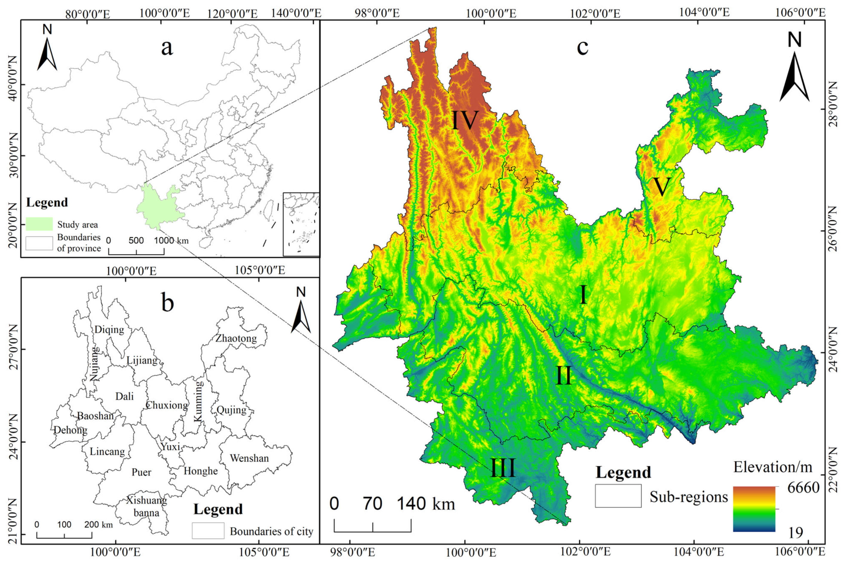
2.1. Study Area

YP is a key component of the “two screens and three belts” ecological security strategy in China. It is on the southwestern border of China, between 97°31′ E and 106°11′ E and between 21°8′ N and 29°15′ N and has an area of ~39.41 × 10⁴ km² (Figure 1). The province has a complex terrain with high mountain valleys to the west and plateaus to the east. The complex terrain leads to an obvious three-dimensional climate. Northwest Yunnan falls within a frigid climate zone, central and east Yunnan fall into a temperate climate zone, and southern and west Yunnan are in the geothermal valley area.

The complex topography, natural climate, soil conditions, ethnicity, and history of YP have led to the different characteristics of the five different planting areas in YP. Most of the Central Yunnan Plateau Basin Zone belongs to the subtropical and warm temperate climate types, with gentle terrain, numerous lakes, and superior agricultural production conditions. Most of the South Yunnan Central Mountain and Broad Valley Zone has a subtropical and mid-subtropical climate. The terrain descends slowly from northwest to southeast, and there are abundant forest resources. The Southern Border Low Mountain Zone has a hot and humid climate and low terrain, with superior natural conditions, and mainly develops tropical crops. The Northwest Yunnan Alpine Valley Zone in northwestern Yunnan has a cold climate and the lowest level of crop yields. The topography and landforms of the Northeast Yunnan Mountain Plain Zone are complex, the climate is significantly different, the distribution of crops has obvious “three-dimensionality”, and it is easily affected by natural disasters. For the convenience of subsequent analysis, we named the above five regions Sub-region I, Sub-region II, Sub-region III, Sub-region IV, and Sub-region V, respectively.

2.2. Data Sources

Basic geographic data, LULC data, NPP data, soil data, meteorological data, DEM data, and socioeconomic data were among the types of data we used. (1) The basic geographic data were derived from the China National Geographic Information Resources Catalogue Service System (https://www.webmap.cn/, accessed on 5 August 2023) at a scale of 1:1 million. (2) LULC data were taken from the GLC_FCS 30 dataset with 30 m spatial resolution [36]. (3) The NPP data were derived from two different datasets: the NPP data from 1990 to 2010 were derived from the ChinaNPP_1985_2015 [37] and the NPP data in 2020 were derived from MOD17A3, which have spatial resolution of 1 km and 500 m, respectively. Due to differences in spatial resolution and data extent between the two datasets, the NPP data in 2020 were corrected through regression analysis and resampling. (4) Soil data include soil type and soil conservation data, of which soil type data were derived from the Harmonized World Soil Database (HWSD) at a scale of 1:1 million and soil conservation data were derived from the China Soil Conservation Data (CSCD) at a spatial granularity of 300 m [38]. (5) Meteorological data were derived from China’s 1 km monthly precipitation/average temperature dataset (1901–2022) [39]. (6) DEM data were derived from ASTER GEDM with 30 m spatial resolution, obtained from Geospatial Data Cloud (http://www.gscloud.cn/, accessed on 12 August 2023). (7) Socioeconomic data included data on population density, grain production, and grain planting area in YP, with population density data downloaded from the Data Centre for Resource and Environmental Sciences of the Chinese Academy of Sciences (http://www.resdc.cn, accessed on 20 August 2023) and grain production data sourced from the Yunnan Provincial Statistical Yearbook.

2.3. Methods

Figure 2 shows the process used in the present study to calculate ESV for the study area. There were the main steps: (1) the construction of dynamic ESV equivalence tables for different sub-regions of YP based on socioeconomic data, NPP, precipitation, soil conservation data, and the Chinese ESV base equivalence table; (2) the calculation of ESV for YP using the EFM, and an analysis of its spatio-temporal evolution, spatial autocorrelation, and response to LUCC; and (3) the simulation of the ESV of YP in 2030 through the PLUS model.

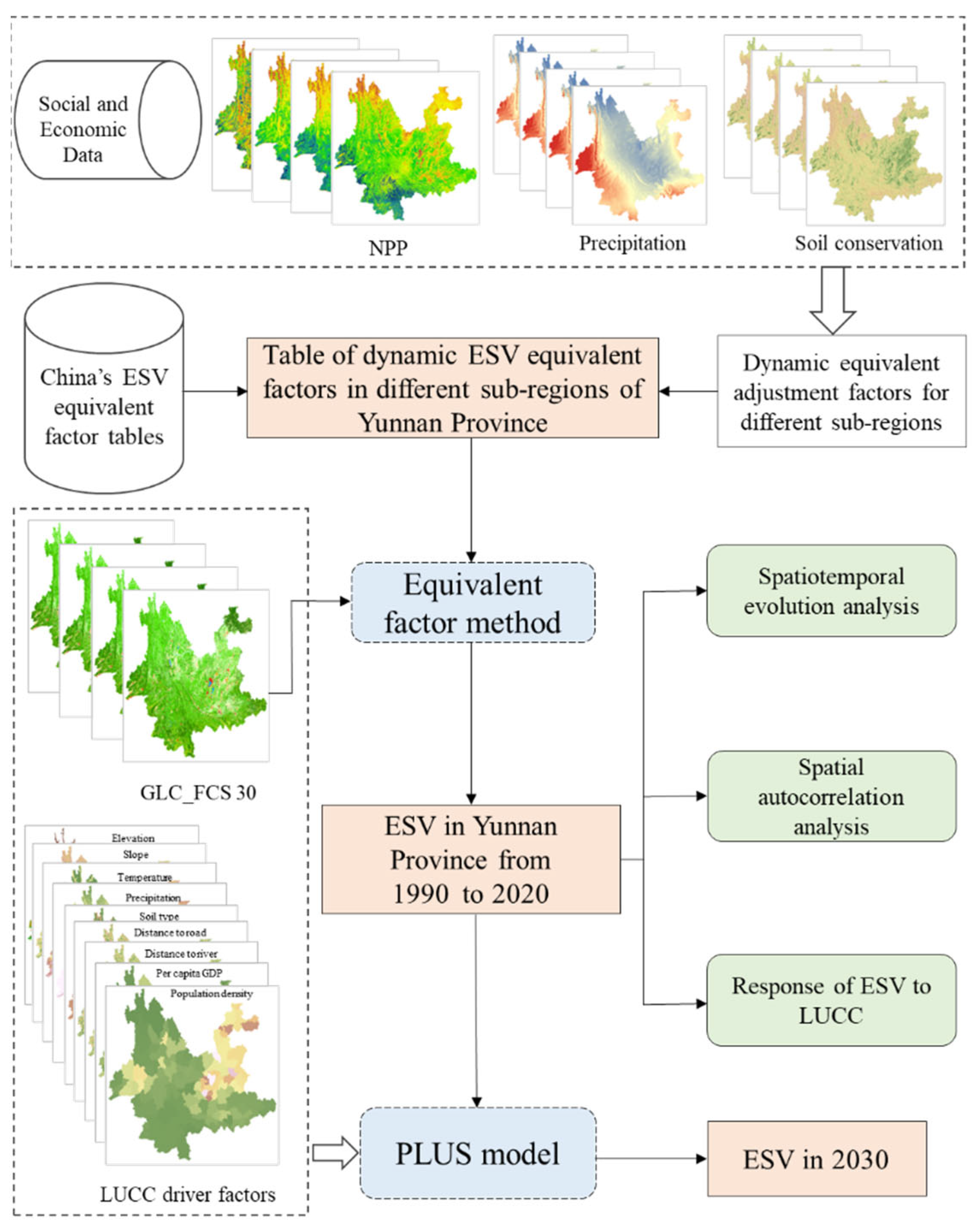
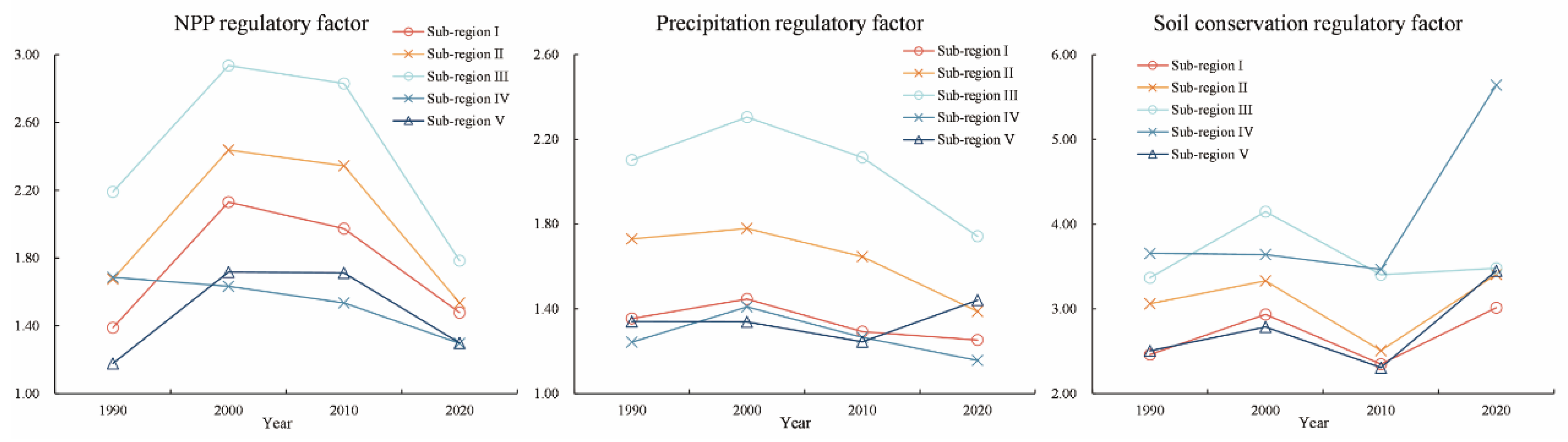
2.3.1. Construction of Dynamic ESV Equivalent Tables

The Chinese ESV Equivalent Table, which Xie et al. [30] amended in 2015, served as the foundation for the current work. We revised the table through 4 steps due to the different study areas. Firstly, 1 standard equivalent factor is the economic value of the annual natural grain production from 1 hm² of farmland with the national average yield [31]. Compared with China, there is a large difference in the economic value of the annual natural grain yield of farmland in Yunnan Province, which leads to a large difference in its standard equivalence factor. Therefore, the equivalent factor adjustment coefficient of 0.7 was calculated using the ratios of the Yunnan Province and national-average grain yields per unit of grain from 1990 to 2020.

Secondly, Equation (1) was used to revise the economic value of a standard equivalent factor in different sub-regions of YP. Among them, the principal food crops in the four sub-regions I, II, III, and IV are rice, wheat, and corn while the main food types in Sub-region V are rice, corn, and potato. Value of a standard equivalent factor in different sub-regions from 1990 to 2020 (

Table 1. Value of a standard equivalent factor in different sub-regions from 1990 to 2020 (CNY/hm²).

Sub-Regions	1990	2000	2010	2020
I	1497.11	1895.66	2060.33	2253.36
II	1033.83	1305.55	1440.97	1663.45
III	1235.26	1513.30	1589.53	1654.42
IV	857.28	1179.41	1314.86	1382.57
V	1212.10	1365.67	1711.71	1726.77

) were obtained through the above two procedures.

$$E_a=\frac{1}{7}{\sum }_{i=1}^n\frac{m_i{p}_i{q}_i}{M}$$

(1)

In Equation (1), E_a is the economic value of 1 standard equivalent factor; i represents the type of food crop; m_i, p_i, and q_i are the average price, unit yield, and planting area of the i-th food crop, respectively; and M represents the gross area of food crops.

Thirdly, ESs change over time. Previous studies [31] have shown that several ESs such as food production and raw material of ecosystems are positively correlated with biomass. Precipitation has a significant effect on water supply and hydrological regulation. Precipitation, topography, soil quality, and vegetation cover all have a substantial impact on soil conservation. Therefore, the ESV equivalent in the study area can be dynamically adjusted through NPP, precipitation, and soil conservation (Equation (2)). Among them, the equivalent factors for food production, raw material production, gas regulation, climate regulation, environmental purification, nutrient cycling, biological diversity, and aesthetic value services in the Chinese ESV Equivalent Table were adjusted by the NPP adjustment factor, and these were calculated through Equation (3). The equivalent factors for water supply and water regulation services were adjusted by a precipitation adjustment factor, and these were calculated in Equation (4). The equivalent factor for soil conservation services were adjusted by a soil conservation adjustment factor, calculated as shown in Equation (5). Figure 3 displays the dynamic adjustment variables for NPP, precipitation, and soil conservation in various regions from 1990 to 2020.

Finally, the ESV dynamic equivalent tables of different sub-regions in YP were obtained by multiplying the correction coefficient of the equivalence factor, the value of a standard equivalence factor, and the basic Chinese ESV equivalent table from Xie et al. [30] with different adjustment factors.

$$F_{nij}=\left\{\begin{array}{c}{P}_{ij}\times F_{n1} or\\ R_{ij}\times F_{n2} or\\ S_{ij}\times F_{n3}\end{array}\right.$$

(2)

$$P_{ij}=\frac{B_{ij}}{\overline{B}}$$

(3)

$$R_{ij}=\frac{W_{ij}}{\overline{W}}$$

(4)

$$S_{ij}=\frac{E_{ij}}{\overline{E}}$$

(5)

In Equations (2)–(5), F_nij is the ESV equivalent factor per unit area of the n-th ES type in the j-th region of an ecosystem in the i-year; P_ij, R_ij, and S_ij are the adjustment factors of NPP, precipitation and soil conservation in the j-th region in i-th year, respectively; F_n is the ESV equivalent factor of the n-th ecosystem service; and n₁, n₂ and n₃ are ESs related to NPP, precipitation and soil conservation, respectively. B_ij, E_ij, and E_ij are NPP, precipitation, and soil conservation in the j-th region in i-th year, respectively. $\overline{B}$, $\overline{W,}$ and $\overline{E}$ are the average NPP, average annual precipitation, and average soil conservation in China, respectively.

2.3.2. Estimation of ESV

Based on EFM (Equation (3)) and the dynamic equivalence table of ESV for various sub-regions, the ESV for Yunnan Province was estimated.

$$ESV={\sum }_{i=1}^n{A}_i\times V{C}_i$$

(6)

In Equation (6), i is the ecosystem type, A_i is the area of the i-th ecosystem type, and VC_i is the ESV equivalent factor per unit area of the i-th ecosystem type.

2.3.3. Exploratory Spatial Data Analysis

Spatial autocorrelation is an assessment of the similarities between variables based on their location similarity [40]. The first indicator of spatial autocorrelation was determined to be the Global Moran’s I index [41]. It characterizes the spatial autocorrelation of the whole area and outputs the value. Moran’ s I was in the range [–1, 1], with an I exceeding zero, less than zero, and equal to zero indicating a positive, negative, and no spatial correlation between the variables, respectively. The Global Moran’s I index was calculated using the following equation:

$$I=\frac{n{\sum }_{i=1}^n{\sum }_{j=1}^n{w}_{ij}(x_i-\overline{x})(x_j-\overline{x})}{\left({\sum }_{i=1}^n{\sum }_{j=1}^n{w}_{ij}\right){\sum }_{i=1}^n{(x_i-\overline{x})}^2}$$

(7)

The Getis–Ord Gi* index determines the spatial concentration of entities or regions containing high values [42]. It provides the output on a per-pixel basis. This index could indicate the distribution characteristics of ESVs, namely high-value clusters (hot spots) and low-value clusters (cold spots). A G_i* greater than or less than 0 indicates an aggregation area hot spot or cold spot, respectively:

$$G_i^{*}=\frac{{\sum }_{j=1}^n{w}_{ij}(x_j-\overline{x}){\sum }_{j=1}^n{w}_{ij}}{\sqrt{\left[\frac{\left\{{\sum }_{j=1}^n{x}_j^2\right\}}{n}\right]-{\overline{x}}^2}\sqrt{\frac{[n{\sum }_{j=1}^n{w}_{ij}^2-{\left({\sum }_{j=1}^n{w}_{ij}\right)}^2]}{n-1}}}$$

(8)

In Equations (7) and (8), n is the number of areas divided by the study area, x_i represents the attribute value in the i-th area, x_j represents the attribute value in the j-th area, $\overline{x}$ is the average of all attribute values, and w_ij represents the spatial weight matrix.

2.3.4. ESV Prediction with the PLUS Model

The PLUS model is a grid-based LUCC simulation model that combines a novel strategy for land extension and a multi-type random patch seed-based cellular automaton (CA) model. The PLUS model has been shown to simulate data with a higher accuracy compared with those of similar models [43]. The data input into the PLUS model in the present study included population density, GDP, distance from major roads, distance from major rivers, elevation, slope, average annual temperature, average annual precipitation, and soil type. The probabilities of development of various types of LULC, LULC conversion rules, and neighborhood weights were calculated and set. This study built on previous studies [43,44] and analyses of LUCC transfer matrices in YP, and it was set that all LULC types could be transferred to each other under natural development conditions. Among these, the neighborhood weights of rainfed cropland, irrigated cropland, broadleaved forest, needle-leaved forest, shrubland, grassland, wetlands, impervious surfaces, bare areas, water body, and permanent ice and snow were 0.9, 0.1, 0.9, 0.7, 0.1, 0.4, 0.1, 0.2, 0.1, 0.1, and 0.1, respectively.

The LULC data for the study area in 2010, as well as the development probability, transfer cost matrix, and neighborhood weights of various LULC classes, were used to simulate LULC data for 2020. The simulated LULC data were compared with observed data (Figure 4). The results of the simulation had a Kappa coefficient of 0.86, and overall accuracy was 89.65%. These results indicated that the PLUS model performs well in simulating LULC in YP.

3. Results

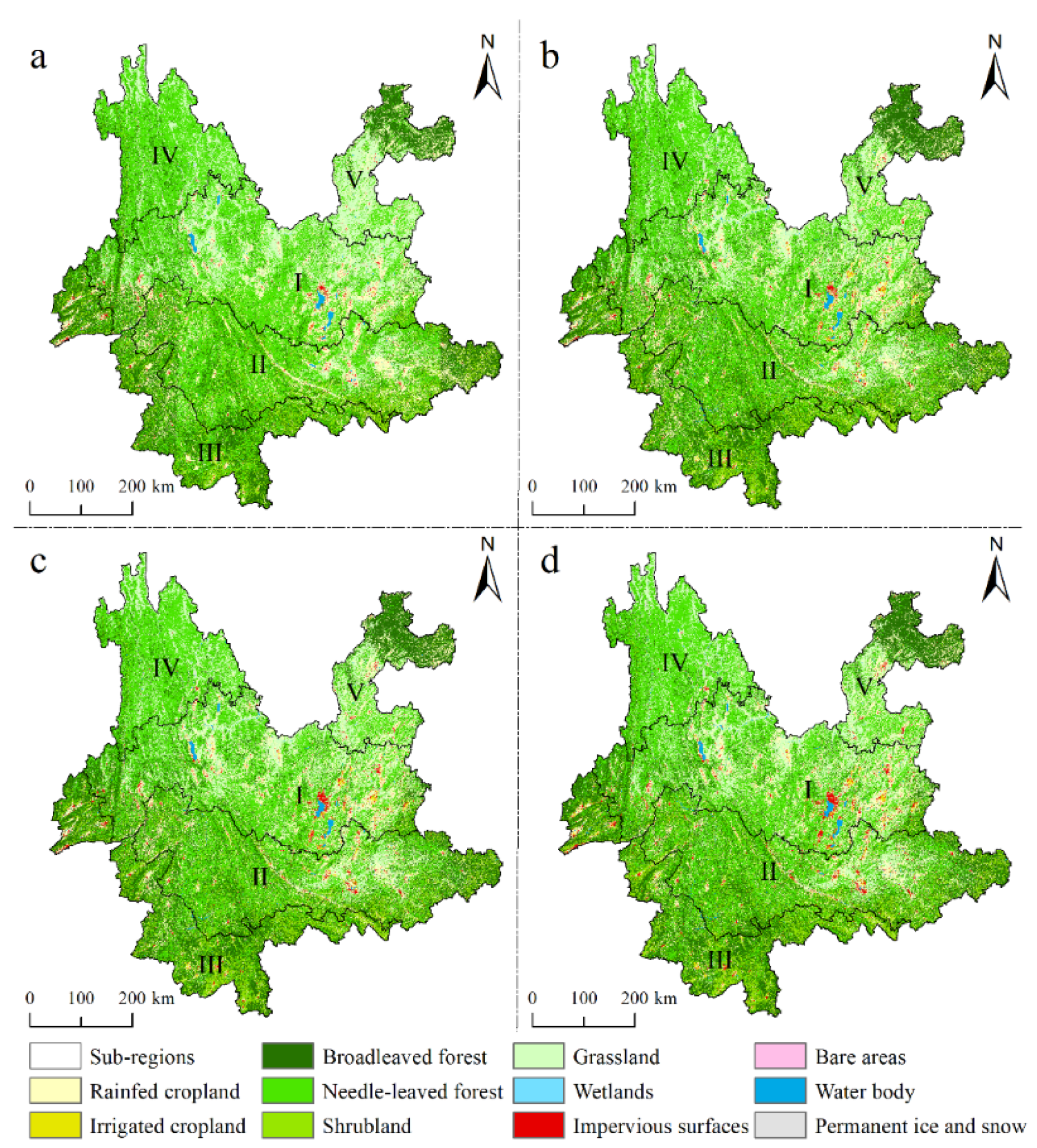
3.1. LUCC in YP from 1990 to 2020

From the perspective of the area of LUCC in YP (Figure 5a), the LULC in YP was dominated by needle-leaved forest, broadleaved forest, grassland, and rainfed cropland, collectively comprising more than 85% of YP’s total LULC area (36.62%, 24.33%, 15.71%, and 13.22%, respectively) (Figure 5). The area of rainfed cropland in YP fluctuated and decreased, with an average annual reduction of 24.74 km². The areas of irrigated cropland and broadleaved forest fluctuated and increased, with average annual increases of 56.84 km² and 516.81 km², respectively. The areas of needle-leaved forest and grassland continued to decrease at 521.75 km²/yr and 412.66 km²/yr, respectively. The areas of shrubland, wetlands, impervious surfaces, bare areas, water body, and permanent ice and snow continued to expand at 217.94 km²/yr, 0.33 km²/yr, 118.41 km²/yr, 3.79 km²/yr, 38.58 km²/yr and 6.44 km²/yr, respectively.

From the perspective of the area of LUCC in different sub-regions (Figure 5b–d,f), from 1990 to 2020, Sub-regions I, II, and IV were dominated by needle-leaved forest, and their areas were decreasing at the rates of 179.70 km²/yr, 228.35 km²/yr, and 24.28 km²/yr, respectively. The main LULC type in Sub-region III was broadleaved forest, and its area was decreasing at 3.51 km²/yr. In 1990, the main LULC type in Sub-region V was grassland, and from 2000 to 2020, the main LULC type in this region became broadleaved forest, which continued to expand at 91.59 km²/yr.

From the perspective of the area of LUCC in YP (Figure 5a), from 1990 to 2020, rainfed croplands and irrigated croplands were mainly distributed in Kunming, Qujing, northern Chuxiong, and north-eastern Honghe Prefecture in Sub-region I and northwestern Wenshan Prefecture in Sub-region II. (Figure 6). Broadleaved forests were concentrated in northern Zhaotong City in Sub-region V and in Sub-region III. Needle-leaved forests were concentrated in the western parts of Sub-region II and Diqing Prefecture in Sub-region IV. Shrublands and grasslands were mainly distributed in the east of Sub-regions I and II and the south of Sub-region V, mostly around cultivated land. Water bodies was dominated by nine plateau lakes and six water systems. Among them, the Dianchi, Fuxian, Xingyun, Yangzonghai, Qilu, Erhai, Chenghai, and Lugu lakes were in Sub-region I whereas the Yilong lake was in Sub-region II. Impervious surfaces were mainly distributed around the lakes. Permanent ice and snow were mainly distributed in northern Diqing and Nujiang states in Sub-region IV.

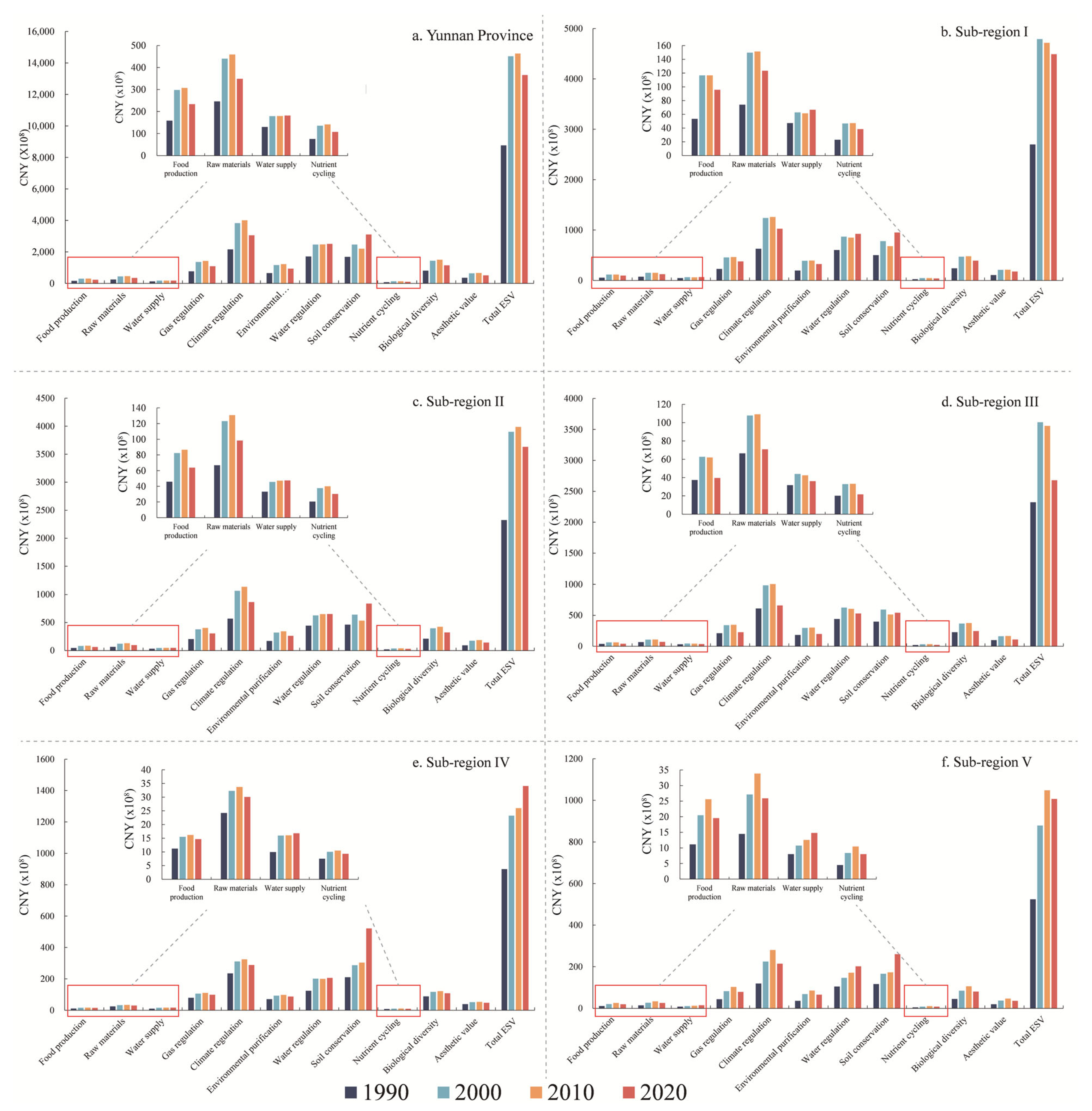
3.2. Characteristics of ESV Changes in YP from 1990 to 2020

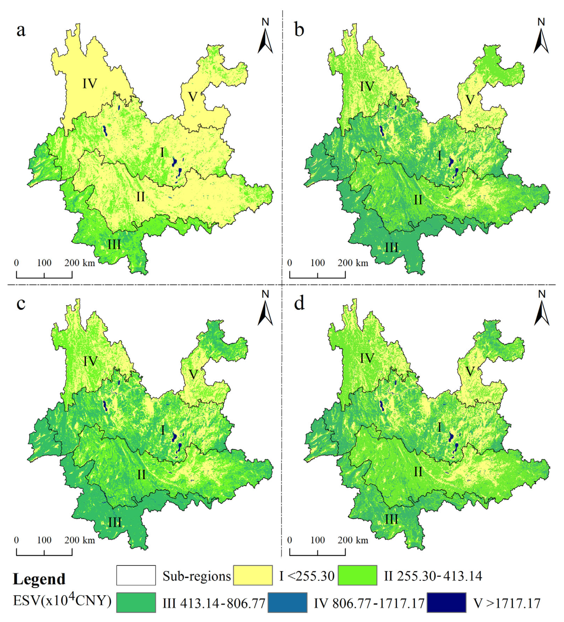
3.2.1. Spatial and Temporal Evolution of ESV in YP

From the perspective of total ESV in YP. The total ESV in YP from 1990 to 2020 fluctuated between CNY 876.74 and 1323.68 B, with a growth rate of 50.98% (Figure 7). The categories could be ranked according to different services’ average contributions to total ESV as follows: climate regulation > soil conservation > water regulation > biological diversity > gas regulation > environmental purification > aesthetic value > raw materials > food production > water supply > maintenance of nutrient cycles (Figure 7). Among them, the values of water supply and water regulation continually increased on average per year by CNY 173.01 M and CNY 2.67 B, respectively. The value of soil conservation fluctuated in an “increase-decrease-increase” trend. The value of all other services increased in a fluctuating “increasing-then-decreasing” trend.

From the perspective of total ESV in different sub-regions, the total ESV in Sub-regions I, II, III, and V increased at fluctuating rates of 5.98 B CNY/yr, 4.36 B CNY/yr, 1.19 B CNY/yr, and 1.61 BCNY/yr, respectively. The value of climate regulation had the highest contribution to total ESV, and its average proportions were 24.67%, 26.06%, 26.59%, and 24.11%, respectively. The total ESV in Sub-region IV continued to grow at 1.77 B CNY/yr, and the value of soil conservation, with an average ratio of 26.63%, made the biggest contribution to the overall ESV.

ESV in YP from 1990 to 2020 increased from east to west (Figure 8). Areas with low ESV (levels I and II) were mainly distributed in the eastern part of Sub-region I, Sub-region II, and Sub-region IV and the middle and south of Sub-region V, especially in Zhaotong City and Honghe Prefecture. The area of level I decreased continuously at 5856.63 km²/yr while the area of level II increased by 93,859.98 km². The areas of median ESV (level III) were mainly located in the western part of Sub-region I and Sub-region III, and these areas fluctuated and decreased at 2675.80 km²/yr. Areas of high ESV (levels IV and V) were concentrated in the Dianchi Lake and Erhai Lake basins in Sub-region I, and their areas increased by 1250.36 km² and 314.64 km², respectively.

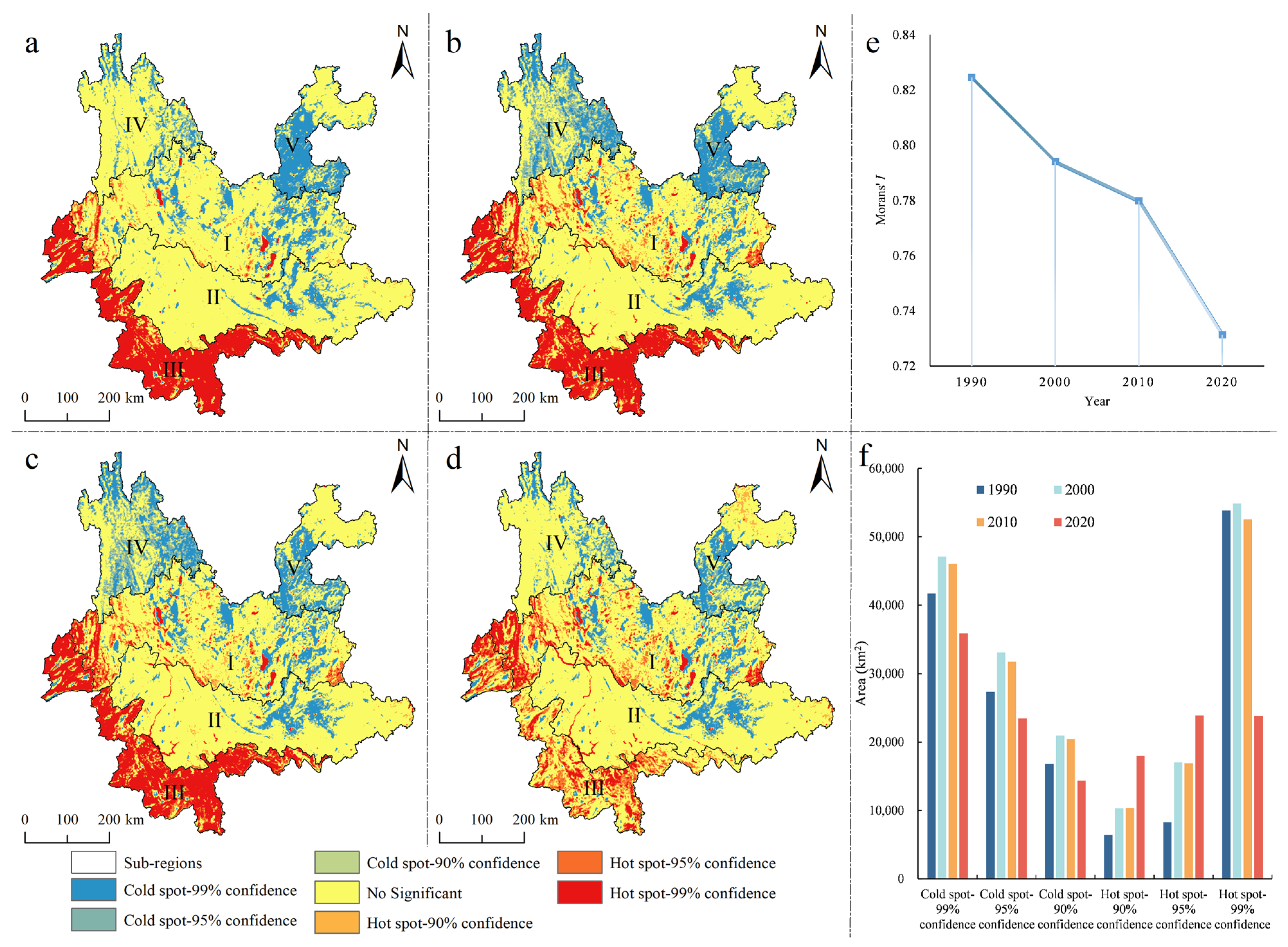
3.2.2. Changes in Spatial Autocorrelation of ESV in YP

The Moran’s I index in YP continued to decline from 1990 to 2020, with the positive spatial correlation gradually weakening (Figure 9e). Sub-region III and the lakes of Sub-region I had the majority of the high-value cluster areas (hot spots) of ESV, accounting for 17.39%, 20.86%, 20.24%, and 16.67% of the total area, respectively. In the northeast of Sub-region IV and in the middle and south of Sub-region V, the low-value cluster (cold spots) of ESV was primarily concentrated, accounting for 21.78%, 25.66%, 24.92%, and 18.68% of the total area, respectively (Figure 9). Over the past 30 years, the area of ESV high- and low-value agglomerations in YP has decreased. However, in our study, the rate of decline of low ESV areas exceeded that of high ESV areas, with their values being 407.08 km²/yr and 95.11 km²/yr, respectively.

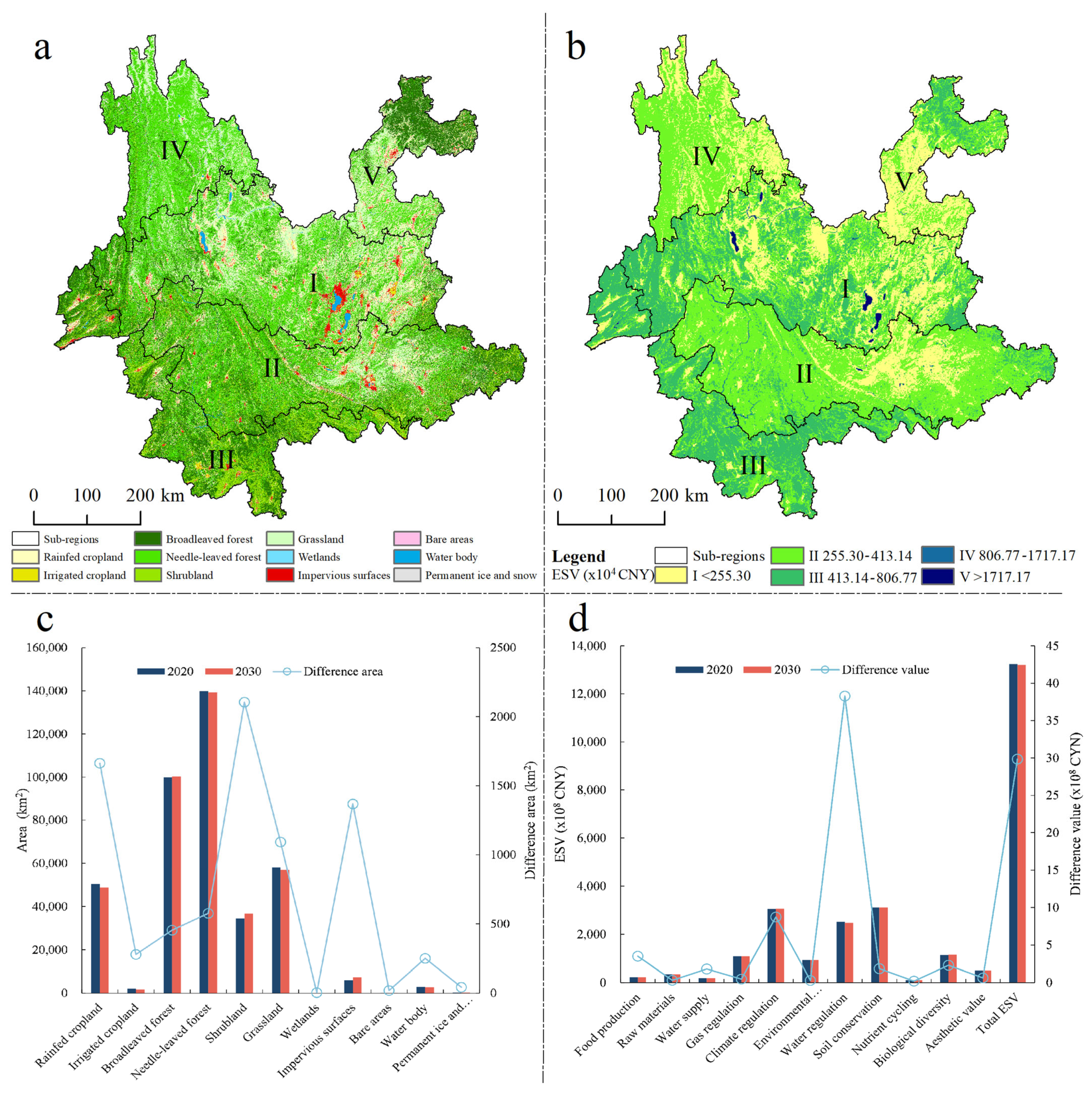
3.3. Prediction of ESV for YP

The spatial distribution of LULC in YP was not dramatically altered in 2030, and needle-leaved forest land was predicted to remain the dominant LULC type in YP in 2030 (Figure 10a). Compared with 2020, the areas of rainfed cropland, irrigated cropland, needle-leaved forest, grassland, wetlands, bare areas, water bodies, and permanent ice and snow were predicted to continue to decrease by 1662.97 km², 278.48 km², 575.81 km², 1092.24 km², 3.74 km², 20.05 km², 249.93 km², and 436.61 km², respectively by 2030. Broadleaf forests, shrublands, and impervious surface expanded rapidly outwards at rates of 45.52 km²/yr, 210.52 km²/yr, and 136.74 km²/yr, respectively (Figure 10c).

The spatial pattern of ESV in YP in 2030 was essentially unchanged from that of 2020 (Figure 10b), and the total ESV slightly decreased by CNY 2.98 B. Among them, the values of food production, raw materials, water supply, water regulation, and nutrient cycling showed a decreasing trend, decreasing by CNY 350.12 M, CNY 31.77 M, CNY 181.72 M, CNY 3.829 B, and CNY 20.41 M, respectively; the values of gas regulation, climate regulation, environmental purification, soil conservation, biological diversity, and aesthetic value showed an increasing trend, increasing by CNY 46.79 M, CNY 873.66 M, CNY 30.42 M, CNY 184.81 M, CNY 231.10 M, and CNY 62.61 M, respectively (Figure 10d).

4. Discussion

4.1. Reliability and Applicability of Research

In terms of methodology, the EFM estimates ESV on the premise that the unit value of each hectare ecosystem type is constant [1]. Costanza et al. [18] showed that the underlying data and models they used to assess global ESV can be applied at multiple scales. At different regional and spatial scales, experts can adjust the values of local ecosystem conditions through differences in local ecological and economic environments [45] to develop a more locally relevant table of value equivalents. The method is widely used in different countries and regions of the world such as central Mexico [46], northern Ethiopia [47], Texas in the USA [48], and the Sundarbans Biosphere Region of India [49]. These large number of cases illustrate the reliability of the method and its applicability in other regions. However, ESs have significant spatial and temporal heterogeneity due to multifactorial influences such as natural substrate conditions, natural hazards, climate change, and LUCC. This effect was less considered in the above studies. Therefore, this study proposed a perspective of ESV assessment based on spatio-temporal heterogeneity. In fact, the methodology of this study was a slight improvement of the EFM, which can be applied to other areas as well. It is important to note that the revised data of the ESV equivalence table need to be adjusted during the method migration process according to the ecosystem characteristics, socioeconomic background, and data availability of the target area to ensure the validity of the assessment method.

In terms of research results, in previous studies on ESs and ESV in YP, Zhang et al. [50] noted that ESV in YP showed an increasing trend from 2000 to 2010. Wang et al. [51] demonstrated that the ESV in YP had been increasing from 2000 to 2020 and that the value of climate control made up the largest portion of YP’s overall ESV. ESV low-value areas were primarily found in the northeast and central of YP whereas ESV high-value areas were primarily found in the northwest and southwest of YP. According to Luo et al. [52], ESV in YP increased gradually between 2005 and 2018, with a pattern of “high in the west, low in the middle, and east”. Wang et al. [53] showed that the spatial distribution of the three ESs of carbon storage, water yield, and habitat quality in YP was “low in the east and high in the west”. The results of this study are highly consistent with all the investigations mentioned above, demonstrating the validity and applicability of the method.

4.2. Effect of LUCC on ESV

LUCC was shown to be a key factor affecting ESV [54,55,56,57]. According to the findings of Xiao et al. [58] and Xing et al. [59], land urbanization would result in a decline in regional ESV. Wang et al. [60] showed a strong positive correlation between LULCC intensity and ESV. Liu et al. [61] demonstrated that the enhancement in ESV in the agro-pastoral interlaced zone in northern China is related to a vegetation restoration project in this region. Total ESV in YP showed a fluctuating increasing trend over time (Figure 7a) that was closely related to LUCC. As can be seen in Figure 11, both in YP and in different sub-regions, for different LULC types, the ESV produced by forests (including broadleaved forest, needle-leaved forest, and shrubland) was the highest. The forest area of YP showed a fluctuating increase from 1990 to 2020. This was due to the implementation of ecological conservation programs like the “Colorful Yunnan Protection Action” and the “Grain for Green” program [50]. Consequently, the ESV in YP showed a rise in volatility from 1990 to 2020. The ecological rehabilitation work of the “Running Yunnan Project” and “returning ponds, returning lakes, and returning wetlands” has provided favorable support for the growth of wetland and water body area in YP. This has led to a gradual increase in ESV for water supply and hydrological regulation. The ESV of other services showed upward trends due to increasing areas in cropland and forestland.

Most of the low-value areas of ESV were located in YP’s eastern part, including the eastern part of Sub-region I, Sub-region II, Sub-region IV, and the middle and south of Sub-region V. The southwest of YP, encompassing the west of Sub-regions I and III, was where the median-value areas of ESV were primarily found. The high-value regions were scattered throughout Sub-region I’s water body areas (Figure 8). This spatial distribution pattern could be mainly attributed to the layout of the LULC. The average ESVs produced by 1 ha of rainfed and irrigated cropland in YP between 1990 and 2020 were CNY 7252.18 and CNY 4893.56, respectively. These values were below those generated by water bodies (CNY 136,866.10), wetlands (CNY 64,887.38), broadleaved forests (CNY 33,634.52), and needle-leaved forests (CNY 25,826.72).

The eastern part of YP, dominated by Sub-region I and Sub-region II, is characterized by a flat terrain, mild climate, abundant water resources, and large population. These conditions are favorable for agriculture, resulting in a concentrated area of cultivated land and a consequent low ESV [58,62]. Sub-region IV was also an area of low ESV. This is because the presence of the Jinsha, Nujiang, and Lancang rivers in northwestern Yunnan along with associated mountains and valleys has created an environment rich in forest resources [50,63]. Insufficient heat resources, poor crop growth conditions, and extensive farming by farmers lead to low production levels of food crops and backward per unit yield, making the equivalent factor of this area’s ESV lower than those of other Sub-regions. Sub-region III had a relatively high ESV. This was because the region is low-lying, being rich in light, heat, water, soil, and biological resources, and its favorable natural conditions provide an excellent environment for tropical plant growth.

4.3. Strategies to Improve ES

Yang et al. [64] identified an increasing trend in forests in YP by 2027. Han et al. [65] predicted that the ecological security of agricultural land in YP would continue to decrease from 2017 to 2025. The above research supports the assertion that the ESV of gas regulation, climate regulation, environmental purification, soil conservation, biological diversity, and aesthetic value in YP will increase and the ESV of food production and raw material will decrease in 2030 (Figure 10d). Given this spatial heterogeneity in ESV, it is important to identify methods of improving ecosystem services in different regions.

The eastern part of YP, dominated by Sub-regions I, II, and V, is experiencing rapid urban expansion, insufficient cropland reserve resources, rocky desertification, and serious soil erosion. Therefore, there is a need to strictly control the boundaries of urban expansion, optimize the use of existing construction land, and guide the layout of cities and towns in suitable mountainous areas. In addition, permanent basic farmland should be promoted; farmland protection should be enforced, particularly in urbanized areas; farmland quality should be improved; and the transition from traditional agricultural production to tourism and leisure agriculture should be facilitated. Also, the policies of “Grain for Green”, improving the quality and quantity of forests, and promoting the restoration of rocky desertification in southeastern Yunnan should be continued. Water sources and wetlands in plateau lake areas such as the Dianchi and Fuxian lakes should be protected.

Northwest Yunnan, dominated by Sub-region IV, is limited by geographical conditions, and this region contains a high proportion of ecologically sensitive areas [66]. Damage to the ecological environment is difficult to reverse. Therefore, forest resource management and biodiversity protection should be strengthened, and a strong ecological buffer zone should be constructed on the “southeast edge of the Qinghai-Tibet Plateau”. In order to increase food yields per unit, farming techniques for crops used for human consumption must also be improved.

Southern Yunnan, dominated by Sub-region III, is rich in forest resources. Therefore, the conservation of forest resources in this area should be strengthened, and the ecological buffer zone of the “southern border” and carbon neutral demonstration areas should be enforced.

4.4. Future Research

This research offers a more precise evaluation of regional ESV from a perspective of spatio-temporal heterogeneity, which will help researchers in providing an appropriate evaluation of ESV in different regions. It is worth noting that the equivalence factor method can be used to rapidly calculate the ESV of a study area. However, this is highly subjective and cannot reflect the complexity and internal mechanism of the ecosystem [67]. Therefore, ESV studies based on ecological models, such as InVEST [68] and Solves [69], are becoming increasingly extensive. Although the above ecological models consider the complexity of the ecosystem, they are often based on a characteristic research area or ecosystem [67]. Future studies should aim to improve the accuracy of ESV assessment. It is possible to use high-resolution remote sensing images to enhance LULC’s classification accuracy further and to couple several models, such as InVEST and the equivalency technique, to gain the advantages of each.

In addition, expressing the ESV in monetary units is an important tool for raising public awareness and communicating the importance of ecosystems to decision makers [70]. At present, ESVs are estimated based on current monetary values. Firstly, the current monetary value is an important indicator of the current economic situation, and the assessment results based on the current monetary value can be directly used in the current policy management, which is more realistic. Furthermore, the estimation of ESV usually involves a longer time scale, with inflation causing changes in the purchasing power of the currency over time. If historical currency values are used to estimate ESV, the rate of inflation needs to be taken into account, which may add to the uncertainty and complexity of the estimation. Therefore, in our study, we used current monetary values to quantify the economic value of the equivalent factor in YP from 1990 to 2020. However, it has to be noted that our study also predicted the ESV of YP in 2030 based on the current monetary value, and did not take into account future economic changes and inflation, which may underestimate the future ESV. Future studies could use inflation rates or other economic indicators to adjust the predictions.

5. Conclusions

Spatio-temporal heterogeneity is an important factor influencing the accurate assessment of ESV in large-scale regions, but most previous studies have ignored the effect. In order to overcome this deficiency, we have proposed a new perspective on regional ESV estimation based on the spatio-temporal heterogeneity of ES, which can accurately estimate the ESV in different sub-regions of the study area. The results of our study show that LULC in YP from 1990 to 2020 was dominated by needle-leaved forest, broadleaved forest, grassland, and rainfed cropland. Total ESV in YP from 1990 to 2020 fluctuated and increased at 14.90 B CNY/yr. ESV increased from east to west. ESV fluctuated due to the YP forest’s fluctuating development, and its spatial distribution was controlled by the LULC pattern. The value of climate regulation made up the largest portion of the total ESV of all the services. ESV had a significant positive spatial correlation, but this correlation was gradually weakening. In 2030, the total ESV of YP decreased slightly by CNY 2.98 B, and the spatial pattern did not change significantly.

References

1. Costanza, R.; Arge, R.; Groot, R.; Farber, S.; Grasso, M.; Hannon, B.; Limburg, K.; Naeem, S.; Neill, R.V.O.; Paruelo, J.; et al. The value of the world’s ecosystem services and natural capital. Nature 1997, 387, 253–260. [Google Scholar] [CrossRef]
2. Hasan, S.; Zhen, L.; Miah, M.; Ahamed, T.; Samie, A. Impact of land use change on ecosystem services, A review. Environ. Dev. 2020, 34, 100527. [Google Scholar] [CrossRef]
3. Liu, Z.; Liu, Z.; Zhou, Y.; Huang, Q. Distinguishing the Impacts of Rapid Urbanization on Ecosystem Service Trade-Offs and Synergies, A Case Study of Shenzhen, China. Remote Sens. 2022, 14, 4604. [Google Scholar] [CrossRef]
4. Mancini, M.S.; Galli, A.; Coscieme, L.; Niccolucci, V.; Lin, D.; Pulselli, F.M.; Bastianoni, S.; Marchettini, N. Exploring ecosystem services assessment through Ecological Footprint accounting. Ecosyst. Serv. 2018, 30, 228–235. [Google Scholar] [CrossRef]
5. Bai, X.; Ran, C.; Chen, J.; Luo, G.; Chen, F.; Xiao, B.; Long, M.; Li, Z.; Zhang, X.; Shen, Q.; et al. Methods, progess and prospect for diagnosis of karst ecosystem health in China, An overview. Chin. Sci. Bull. 2023, 68, 2550–2568. [Google Scholar]
6. Nie, X.; Wang, Q.; Wu, J.; Wang, H.; Chen, Z.; He, J. Effectively enhancing perceptions of cultural ecosystem services, A case study of a karst cultural ecosystem. J. Environ. Manag. 2022, 315, 115189. [Google Scholar] [CrossRef]
7. Gao, J.; Zuo, L.; Liu, W. Environmental determinants impacting the spatial heterogeneity of karst ecosystem services in Southwest China. Land Degrad. Dev. 2020, 32, 1718–1731. [Google Scholar] [CrossRef]
8. Hu, Z.; Wang, S.; Bai, X.; Luo, G.; Li, Q.; Wu, L.; Yang, Y.; Tian, S.; Li, C.; Deng, Y. Changes in ecosystem service values in karst areas of China. Agric. Ecosyst. Environ. 2022, 301, 107026. [Google Scholar] [CrossRef]
9. Zhang, X.; Xie, B.; Zhou, K.; Li, J.; Yuan, C.; Xiao, J.; Xie, J. Mapping ecosystem service clusters and exploring their driving mechanisms in karst peak-cluster depression regions in China. Ecol. Indic. 2023, 158, 111524. [Google Scholar] [CrossRef]
10. Viglizzo, E.F.; Frank, F.C. Land-use options for Del Plata Basin in South America, Tradeoffs analysis based on ecosystem service provision. Ecol. Econ. 2006, 57, 140–151. [Google Scholar] [CrossRef]
11. Tong, C.; Feagin, R.A.; Lu, J.; Zhang, X.; Zhu, X.; Wei, W.; He, W. Ecosystem service values and restoration in the urban Sanyang wetland of Wenzhou, China. Ecol. Eng. 2007, 29, 249–258. [Google Scholar] [CrossRef]
12. Wu, Y.; Jie, C.; Xu, B.; Peng, C.; Ying, G. Ecosystem service value assessment for constructed wetlands, A case study in Hangzhou, China. Ecol. Econ. 2008, 68, 116–125. [Google Scholar] [CrossRef]
13. Jenkins, W.A.; Murray, B.C.; Kramer, R.A.; Faulkner, S.P. Valuing ecosystem services from wetlands restoration in the Mississippi Alluvial Valley. Ecol. Econ. 2010, 69, 1051–1061. [Google Scholar] [CrossRef]
14. Estoque, R.C.; Myint, S.W.; Wang, C.; Ishtiaque, A.; Aung, T.T.; Emerton, L.; Ooba, M.; Hijioka, Y.; Mon, M.S.; Wang, Z.; et al. Assessing environmental impacts and change in Myanmar’s mangrove ecosystem service value due to deforestation (2000–2014). Glob. Chang. Biol. 2018, 24, 5391–5410. [Google Scholar] [CrossRef]
15. Negash, E.; Getachew, T.; Birhane, E.; Gebrewahed, H. Ecosystem Service Value Distribution Along the Agroecological Gradient in North-Central Ethiopia. Earth Syst. Environ. 2020, 4, 107–116. [Google Scholar] [CrossRef]
16. Brown, G.; Hausner, V. An empirical analysis of cultural ecosystem values in coastal landscapes. Ocean. Coast. Manag. 2017, 142, 49–60. [Google Scholar] [CrossRef]
17. Brander, L.; Wagtendonk, A.; Hussain, S.; McVittie, A.; Verburg, P.; de Groot, R.; van der Ploeg, S. Ecosystem service values for mangroves in Southeast Asia, A meta-analysis and value transfer application. Ecosyst. Serv. 2012, 1, 62–69. [Google Scholar] [CrossRef]
18. Costanza, R.; Groot, R.; Sutton, P.; Ploeg, S.; Anderson, S.J.; Kubiszewski, I.; Farber, S.; Turner, R.K. Changes in the global value of ecosystem services. Glob. Environ. Chang. 2014, 26, 152–158. [Google Scholar] [CrossRef]
19. Sannigrahi, S.; Bhatt, S.; Rahmat, S.; Paul, S.K.; Sen, S. Estimating global ecosystem service values and its response to land surface dynamics during 1995–2015. J. Environ. Manag. 2018, 223, 115–131. [Google Scholar] [CrossRef]
20. Cao, S.; Liu, Y.; Su, W.; Zheng, X.; Yu, Z. The net ecosystem services value in mainland China. Sci. China-Earth Sci. 2018, 61, 595–603. [Google Scholar] [CrossRef]
21. Baniya, B.; Tang, Q.; Pokhrel, Y.; Xu, X. Vegetation dynamics and ecosystem service values changes at national and provincial scales in Nepal from 2000 to 2017. Environ. Dev. 2019, 32, 100464. [Google Scholar] [CrossRef]
22. Kubiszewski, I.; Costanza, R.; Dorji, L.; Thoennes, P.; Tshering, K. An initial estimate of the value of ecosystem services in Bhutan. Ecosyst. Serv. 2013, 3, E11–E21. [Google Scholar] [CrossRef]
23. Remme, R.; Edens, B.; Schroter, M. Monetary accounting of ecosystem services, A test case for Limburg province, the Netherlands. Ecol. Econ. 2015, 112, 116–128. [Google Scholar] [CrossRef]
24. Immerzeel, B.; Vermaat, J.; Riise, G.; Juutinen, A.; Futter, M. Estimating societal benefits from Nordic catchments, An integrative approach using a final ecosystem services framework. PLoS ONE 2021, 16, e0252352. [Google Scholar] [CrossRef]
25. Li, T.; Li, W.; Qian, Z. Variations in ecosystem service value in response to land use changes in Shenzhen. Ecol. Econ. 2010, 69, 1427–1435. [Google Scholar] [CrossRef]
26. Nikodinoska, N.; Paletto, A.; Pastorella, F.; Granvik, M.; Franzese, P. Assessing, valuing and mapping ecosystem services at city level, The case of Uppsala (Sweden). Ecol. Model. 2018, 368, 411–424. [Google Scholar] [CrossRef]
27. Zhang, H.; Yang, Q.; Zhang, Z.; Lu, D. Spatiotemporal Changes of Ecosystem Service Value Determined by National Land Space Pattern Change, A Case Study of Fengdu County in The Three Gorges Reservoir Area, China. Int. J. Environ. Res. Public Health 2021, 18, 5007. [Google Scholar] [CrossRef]
28. Liu, Y.; Li, J.; Yang, Y. Evaluation of forest ecosystem services based on biomass in Shanxi Province. Acta Ecol. Sin. 2012, 32, 2699–2706. [Google Scholar]
29. Stoeckl, N.; Condie, S.; Anthony, K. Assessing changes to ecosystem service values at large geographic scale, A case study for Australia’s Great Barrier Reef. Ecosyst. Serv. 2021, 51, 101352. [Google Scholar] [CrossRef]
30. Xie, G.; Zhang, C.; Zhang, L.; Chen, W.; Li, S. Improvement of the Evaluation Method for Ecosystem Service Value Based on Per Unit Area. J. Nat. Resour. 2015, 30, 1243–1254. [Google Scholar]
31. Xie, G.; Zhen, L.; Lu, C.; Xiao, Y.; Chen, C. Expert Knowledge Based Valuation Method of Ecosystem Services in China. J. Nat. Resour. 2008, 5, 911–919. [Google Scholar]
32. Pan, H.; Zhang, Q.; Li, J.; Xu, J.; Huang, P. Spatial and temporal evolution of ecosystem service value based on dynamic equivalent in Yi-Han severely impoverished areas. Acta Ecol. Sin. 2020, 40, 8218–8229. [Google Scholar]
33. Holland, R.; Eigenbrod, F.; Armsworth, P.; Anderson, B.; Thomas, C.; Gaston, K. The influence of temporal variation on relationships between ecosystem services. Biodivers. Conserv. 2011, 20, 3285–3294. [Google Scholar] [CrossRef]
34. Xie, G.; Zhang, C.; Zheng, L.; Zhang, L. Dynamic changes in the value of China’s ecosystem services. Ecosyst Serv. 2017, 26, 146–154. [Google Scholar] [CrossRef]
35. Wang, J.; Liu, F.; Bai, X.; Dai, W.; Li, Q. The spatial and temporal evolution and simulation forecast of ecosystem service values in southwest China. Acta Ecol. Sin. 2019, 39, 7057–7066. [Google Scholar]
36. Zhang, X.; Liu, L.; Chen, X.; Gao, Y.; Mi, Y. GLC_FCS30, Global land-cover product with fine classification system at 30€m using time-series Landsat imagery. Earth Syst. Sci. Data 2021, 13, 2753–2776. [Google Scholar] [CrossRef]
37. Chen, P. Monthly NPP dataset covering China’s terrestrial ecosystems at north of 18°N (1985–2015). J. Glob. Chang. Data Discov. 2019, 3, 34–41+143–150. [Google Scholar]
38. Li, J.; He, H.; Zeng, Q.; Chen, L.; Sun, R. A Chinese soil conservation dataset preventing soil water erosion from 1992 to 2019. Sci. Data 2023, 10, 319. [Google Scholar] [CrossRef]
39. Peng, S.; Ding, Y.; Liu, W.; Li, Z. 1 km monthly temperature and precipitation dataset for China from 1901 to 2017. Earth Syst. Sci. Data 2019, 11, 1931–1946. [Google Scholar] [CrossRef]
40. Huo, X.; Li, H.; Sun, D.; Zhou, L.; Li, B. Combining Geostatistics with Moran’s I Analysis for Mapping Soil Heavy Metals in Beijing, China. Int. J. Environ. Res. Public Health 2012, 9, 995–1017. [Google Scholar] [CrossRef]
41. Aghadadashi, V.; Molaei, S.; Mehdinia, A.; Mohammadi, J.; Moeinaddini, M.; Bakhtiari, A.R. Using GIS, geostatistics and Fuzzy logic to study spatial structure of sedimentary total PAHs and potential eco-risks; An Eastern Persian Gulf case study. Mar. Pollut. Bull. 2019, 49, 110489. [Google Scholar] [CrossRef]
42. Catchpole, S.; Rivera, R.; Hernández, C.; De La Pena, J.; Conzalez, P. Predicting spatial distribution patterns and hotspots of fish assemblage in a coastal basin of the central-south of Chile, by geostatistical techniques. J. Limnol. 2019, 78, 220–232. [Google Scholar] [CrossRef]
43. Liang, X.; Guan, Q.; Clarke, C.; Liu, S.; Wang, B.; Yao, Y. Understanding the drivers of sustainable land expansion using a patch-generating land use simulation (PLUS) model, A case study in Wuhan, China. Comput. Environ. Urban Syst. 2021, 85, 101569. [Google Scholar] [CrossRef]
44. Wang, Q.; Wang, H.; Chang, R.; Zeng, H.; Bai, X. Dynamic simulation patterns and spatiotemporal analysis of land-use/land-cover changes in the Wuhan metropolitan area, China. Ecol. Model. 2022, 464, 109850. [Google Scholar] [CrossRef]
45. Costanza, R.; Groot, R.; Braat, L.; Kubiszewski, I.; Fioramonti, L.; Sutton, P.; Farber, S.; Grasso, M. Twenty years of ecosystem services, How far have we come and how far do we still need to go? Ecosyst. Serv. 2017, 28, 1–16. [Google Scholar] [CrossRef]
46. Mendoza-González, G.; Martínez, M.L.; Lithgow, D.; Pérez-Maqueo, O.; Simonin, P. Land use change and its effects on the value of ecosystem services along the coast of the Gulf of Mexico. Ecol. Econ. 2012, 82, 23–32. [Google Scholar] [CrossRef]
47. Solomon, N.; Segnon, A.C.; Birhane, E. Ecosystem Service Values Changes in Response to Land-Use/Land-Cover Dynamics in Dry Afromontane Forest in Northern Ethiopia. Int. J. Environ. Res. Public Health 2019, 16, 4653. [Google Scholar] [CrossRef]
48. Yi, H.; Gueneralp, B.; Filippi, A.M.; Kreuter, U.P.; Guneralp, I. Impacts of Land Change on Ecosystem Services in the San Antonio River Basin, Texas, from 1984 to 201. Ecol. Econ. 2017, 135, 125–135. [Google Scholar] [CrossRef]
49. Sannigrahi, S.; Chakraborti, S.; Joshi, P.K.; Keesstra, S.; Sen, S.; Paul, S.K.; Kreuter, U.; Sutton, P.C.; Jha, S.; Dang, K.B. Ecosystem service value assessment of a natural reserve region for strengthening protection and conservation. J. Environ. Manag. 2019, 244, 208–227. [Google Scholar] [CrossRef]
50. Zhang, H.; Liao, X.; Zhai, T. Evaluation of ecosystem service based on scenario simulation of land use in Yunnan Province. Phys. Chem. Earth 2018, 104, 58–65. [Google Scholar] [CrossRef]
51. Wang, F.; Fu, W.; Chen, J. Spatial–Temporal Evolution of Ecosystem Service Value in Yunnan Based on Land Use. Land 2022, 11, 2217. [Google Scholar] [CrossRef]
52. Luo, R.; Chen, X.; Zhang, L.; Yang, W. Spatial-temporal Evolution of Ecosystem Service Value of Counties in YP Based on Land Utilization. J. Anhui Agric. Sci. 2022, 50, 45–48+85. [Google Scholar]
53. Wang, R.; Zhao, J.; Chen, G.; Lin, Y.; Yang, A.; Cheng, J. Coupling PLUS–InVEST Model for Ecosystem Service Research in Yunnan Province, China. Sustainability 2022, 15, 271. [Google Scholar] [CrossRef]
54. Bryan, B.; Ye, Y.; Zhang, J.; Connor, J. Land-use change impacts on ecosystem services value, Incorporating the scarcity effects of supply and demand dynamics. Ecosyst. Serv. 2018, 32, 144–157. [Google Scholar] [CrossRef]
55. Pérez-Ramírez, I.; Requena-Mullor, J.; Castro, A.; García-Llorente, M. Land transformation changes people’s values of ecosystem services in Las Vegas agrarian landscapes of Madrid Spain. Land Use Policy 2023, 134, 106921. [Google Scholar] [CrossRef]
56. Sun, C.; Ma, Y.; Gong, L. Response of ecosystem service value to land use/cover change in the northern slope economic belt of the Tianshan Mountains, Xinjiang, Chin. J. Arid. Land 2021, 13, 1026–1040. [Google Scholar] [CrossRef]
57. Zhang, J.; Li, X.; Zhang, C.; Yu, L.; Wang, J.; Wu, X.; Hu, Z.; Zhai, Z.; Li, Q.; Wu, G.; et al. Assessing spatiotemporal variations and predicting changes in ecosystem service values in the Guangdong-Hong Kong-Macao Greater Bay Area. Gisci. Remote Sens. 2022, 59, 184–199. [Google Scholar] [CrossRef]
58. Xiao, W. Remote Sensing Monitoring of Cropland Change for the Recently 10 Years in Yunnan Based on GEE Platform; Yunnan Normal University: Kunming, China, 2020. [Google Scholar] [CrossRef]
59. Xing, L.; Zhu, Y.; Wang, J. Spatial spillover effects of urbanization on ecosystem services value in Chinese cities. Ecol. Indic. 2021, 121, 107028. [Google Scholar] [CrossRef]
60. Wang, Y.; Ding, J.; Li, X.; Zhang, J.; Ma, G. Impact of LUCC on ecosystem services values in the Yili River Basin based on an intensity analysis model. Acta Ecol. Sin. 2022, 42, 3106–3118. [Google Scholar]
61. Liu, M.; Jia, Y.; Zhao, J.; Shen, Y.; Pei, H.; Zhang, H.; Li, Y. Revegetation projects significantly improved ecosystem service values in the agro-pastoral ecotone of northern China in recent 20 years. Sci. Total Environ. 2021, 788, 147756. [Google Scholar] [CrossRef]
62. Deng, Y. Research on Land Cover Classification in YP Based on MODIS Data; Yunnan Normal University: Kunming, China, 2015. [Google Scholar]
63. Han, T.; Xi, X.; Wang, C.; Bao, Y.; Luo, S. Study on Forest Classification in Yunnan based on Decision Tree Algorithm. Remote Sens. Technol. Appl. 2014, 29, 744–751. [Google Scholar]
64. Yang, Y.; Huang, G.; Wang, X.; Su, H.; Zhi, C. Research on Prediction of Forest Resources and the Carbon Sequestration Potential in Yunnan Pronvince. For. Resour. Manag. 2017, 4, 44–49. [Google Scholar] [CrossRef]
65. Han, L.; Pan, Y.; Gao, Q.; Ma, J. Evaluation and Prediction of the Cultivated Land Ecological Security in YP Based on PSR and Unbiased GM (1, 1) Model. Ecol. Econ. 2019, 35, 148–154. [Google Scholar]
66. Nong, L. Evaluation of Ecological Vulnerability Evaluation of Yunnan Province Based on SPR Model; Yunnan Normal University: Kunming, China, 2021. [Google Scholar]
67. Deng, C.; Liu, J.; Li, Z.; Xiao, H.; Nie, X. Review and Analysis of Ecosystem Services Research between Domestic and Foreign in Recent 20 Years. Ecol. Environ. Sci. 2019, 28, 2119–2128. [Google Scholar] [CrossRef]
68. Sánchez-Canales, M.; Benito, L.; Passuello, A.; Terrado, M.; Ziv, G.; Acuna, V.; Schuhmacher, M.; Elorza, F. Sensitivity analysis of ecosystem service valuation in a Mediterranean watershed. Sci. Total Environ. 2012, 440, 140–153. [Google Scholar] [CrossRef]
69. Sherrouse, B.C.; Semmens, D.J.; Ancona, Z.H.; Brunner, N.M. Analyzing land-use change scenarios for trade-offs among cultural ecosystem services in the Southern Rocky Mountains. Ecosyst. Serv. 2017, 26, 431–444. [Google Scholar] [CrossRef]
70. de Groot, R.; Brander, L.; Ploeg, S.; Costanza, R.; Bernard, F.; Braat, L.; Christie, M.; Crossman, N.; Ghermandi, A.; Hein, L. Global estimates of the value of ecosystems and their services in monetary units. Ecosyst. Serv. 2012, 1, 50–61. [Google Scholar] [CrossRef]
Figure 1. Map of YP, China: (a) administrative divisions of China, (b) administrative regions of YP, and (c) digital elevation model (DEM) of YP, I–V represent sub-region I to sub-region V, respectively.
Land 13 00812 g001
Figure 2. Process used in the present study to calculate the ESV of YP, China.
Land 13 00812 g002
Figure 3. Dynamic adjustment factors of NPP, precipitation, and soil conservation.
Land 13 00812 g003
Figure 4. Comparison of LULC in YP in 2020: (a) actual LULC; (b) modeled LULC. I–V represent sub-region I to sub-region V, respectively.
Land 13 00812 g004
Figure 5. Area of different LULC types in the study area from 1990 to 2020: (a) YP, (b) Sub-region I, (c) Sub-region II, (d) Sub-region III, (e) Sub-region IV, (f) Sub-region V.
Land 13 00812 g005
Figure 6. Spatial distribution of LULC types in YP: (a) 1990, (b) 2000, (c) 2010, (d) 2020. I–V represent sub-region I to sub-region V, respectively.
Land 13 00812 g006
Figure 7. ESV in the study area from 1990 to 2020: (a) YP, (b) Sub-region I, (c) Sub-region II, (d) Sub-region III, (e) Sub-region IV, (f) Sub-region V.
Land 13 00812 g007
Figure 8. Spatial distribution of ecosystem service value (ESV) in YP, China: (a) 1990, (b) 2000, (c) 2010, and (d) 2020. I–V represent sub-region I to sub-region V, respectively.
Land 13 00812 g008
Figure 9. Spatial autocorrelation of ESV in YP: (a) 1990, (b) 2000, (c) 2010, and (d) 2020; (e) Moran’s I and (f) areas of cold and hot spots. I–V represent sub-region I to sub-region V, respectively.
Land 13 00812 g009
Figure 10. Spatial distribution and area of LULC and ESV in YP, China in 2030: (a) spatial distribution of LULC, (b) spatial distribution of ESV, (c) LULC area, and (d) ESV. I–V represent sub-region I to sub-region V, respectively.
Land 13 00812 g010
Figure 11. ESVs for different LULCs in YP, China from 1990 to 2020: (a) YP, (b) different sub-regions.
Land 13 00812 g011