Abstract
Drylands are characterized by unique ecosystem types, sparse vegetation, fragile environments, and vital ecosystem services. The accurate mapping of dryland ecosystems is essential for their protection and restoration, but previous approaches primarily relied on modifying land use data derived from remote sensing, lacking the direct utilization of latest remote sensing technologies and methods to map ecosystems, especially failing to effectively identify key ecosystems with sparse vegetation. This study attempts to integrate Google Earth Engine (GEE), random forest (RF) algorithm, multi-source remote sensing data (spectral, radar, terrain, texture), feature optimization, and image segmentation to develop a fine-scale mapping method for an ecologically critical area in northern China. The results showed the following: (1) Incorporating multi-source remote sensing data significantly improved the overall classification accuracy of dryland ecosystems, with radar features contributing the most, followed by terrain and texture features. (2) Optimizing the features set can enhance the classification accuracy, with overall accuracy reaching 91.34% and kappa coefficient 0.90. (3) User’s accuracies exceeded 90% for forest, cropland, and water, and were slightly lower for steppe and shrub-steppe but were still above 85%, demonstrating the efficacy of the GEE and RF algorithm to map sparse vegetation and other dryland ecosystems. Accurate dryland ecosystems mapping requires accounting for regional heterogeneity and optimizing sample data and feature selection based on field surveys to precisely depict ecosystem patterns in complex regions. This study precisely mapped dryland ecosystems in a typical dryland region, and provides baseline data for ecological protection and restoration policies in this region, as well as a methodological reference for ecosystem mapping in similar regions.
1. Introduction
Drylands account for over 40% of the global terrestrial surface area and support more than one-third of the global population [1]. These water-scarce regions with sparse vegetation, low productivity, and fragile environments play an indispensable role in maintaining global biodiversity, regulating climate, and providing essential ecosystem services [2,3]. However, driven by the demand for economic development, drylands are increasingly becoming hotspots for pursuing “increased productivity” [4,5], posing severe threats to their delicate ecosystems. In China, drylands cover a vast area stretching from the northwest to the north and face severe challenges such as desertification, soil erosion, and vegetation degradation, exacerbated by climate change and intensified human activity [6].
Accurately mapping and continuously monitoring the spatial and temporal distribution patterns of dryland ecosystems are crucial for protecting these fragile regions and enhancing their resistance and resilience to various disturbances [6]. Early ecosystem mapping mainly relied on field surveys and manual interpretation [7,8], which were inefficient, costly, and unable to meet the requirements of regular and timely monitoring and mapping [9]. With the advancement of remote sensing technology, mapping the spatial patterns of ecosystems using land use/land cover as the basic unit has been widely adopted in large-scale, ecosystem-related studies [10,11,12]. For instance, Ouyang et al. [13] proposed a remote-sensing-based ecosystem classification framework based on land use classification criteria. Liu et al. [14] also attempted to classify and map China’s ecosystems by integrating land use with vegetation cover, population density, drought index, elevation, slope, and soil type. Such land use-based methods have been effectively applied on a national scale.
However, regional challenges persist, particularly in drylands. Due to the high surface reflectance and significant soil background interference in these areas, sparse vegetation ecosystems cannot be effectively extracted from existing land use data derived from remote sensing, resulting in a significant underestimation of ecosystem diversity and extent [15]. As a result, current research on dryland ecosystem dynamics has predominantly focused on built-up areas [16,17], croplands [18,19], or forests [20,21,22], neglecting the unique ecosystems of sparse vegetation. This oversight hinders a comprehensive understanding of the dynamic structural changes in ecosystems from a spatial pattern perspective. Therefore, it is urgently needed to make direct use of the latest remote sensing technology and methods to map dryland ecosystems and accurately identify various ecosystems, including sparse vegetation.
Since the advent of the Google Earth Engine (GEE) [23,24], its cloud-based big data processing capabilities, continuously expanding multi-source remote sensing datasets, and integration of advanced machine learning algorithms have paved a new technical path for precisely mapping dryland ecosystems. GEE integrates large-scale geospatial big data from around the globe, including satellite imagery, terrain, climate, and population data. Additionally, these massive datasets can be efficiently stored and processed, thereby overcoming traditional technical bottlenecks [23]. Furthermore, GEE incorporates various machine learning algorithms such as random forest (RF) [25], support vector machine (SVM) [26], and classification and regression trees (CART) [27], which can flexibly leverage multi-source, multi-dimensional data and integrate features at different scales, providing powerful feature representation capabilities for ecosystem mapping in complex and heterogeneous environments [25]. By fully utilizing the GEE’s data processing and analysis capabilities, in combination with remote sensing techniques and machine learning algorithms, we can aspire to obtain accurate dryland ecosystem maps, providing scientific evidence for the protection and sustainable utilization of these fragile regions.
Based on this, a highly representative dryland region in northern China was selected as a case study area to conduct ecosystem mapping research integrating the GEE, machine learning algorithms, multi-source remote sensing data, and object-based segmentation, among other cutting-edge approaches. This region, located in the Yellow River Basin, spans arid, semi-arid, and dry sub-humid zones, featuring a heterogeneous landscape characterized by deserts, Gobi, oases, steppes, and mountains, making it highly representative of global drylands. Furthermore, this region is a priority area in China’s fight against desertification, biodiversity conservation, and related policy initiatives. Moreover, a series of ecological engineering projects implemented in this region, such as the Three-North Shelterbelt Program, Beijing–Tianjin Sandstorm Source Control Project, Natural Forest Protection Program, Returning Farmland to Forest Program, and Returning Grazing Land to Grassland Program, have profoundly altered the ecosystems. Accurate ecosystem mapping in this area is essential for evaluating and guiding these efforts. The hypothesis of this study is that by leveraging GEE and the random forest algorithm, accurate mapping of dryland ecosystems, including sparse vegetation types, can be achieved. Through exploring the applicability of the GEE and RF algorithm for mapping dryland ecosystems, analyzing the impact of different features on mapping accuracy, and summarizing issues that need to be considered during the mapping process, we can provide scientific evidence to inform dryland ecosystem mapping and ecological environment protection policies.
2. Materials and Methods
2.1. Study Area
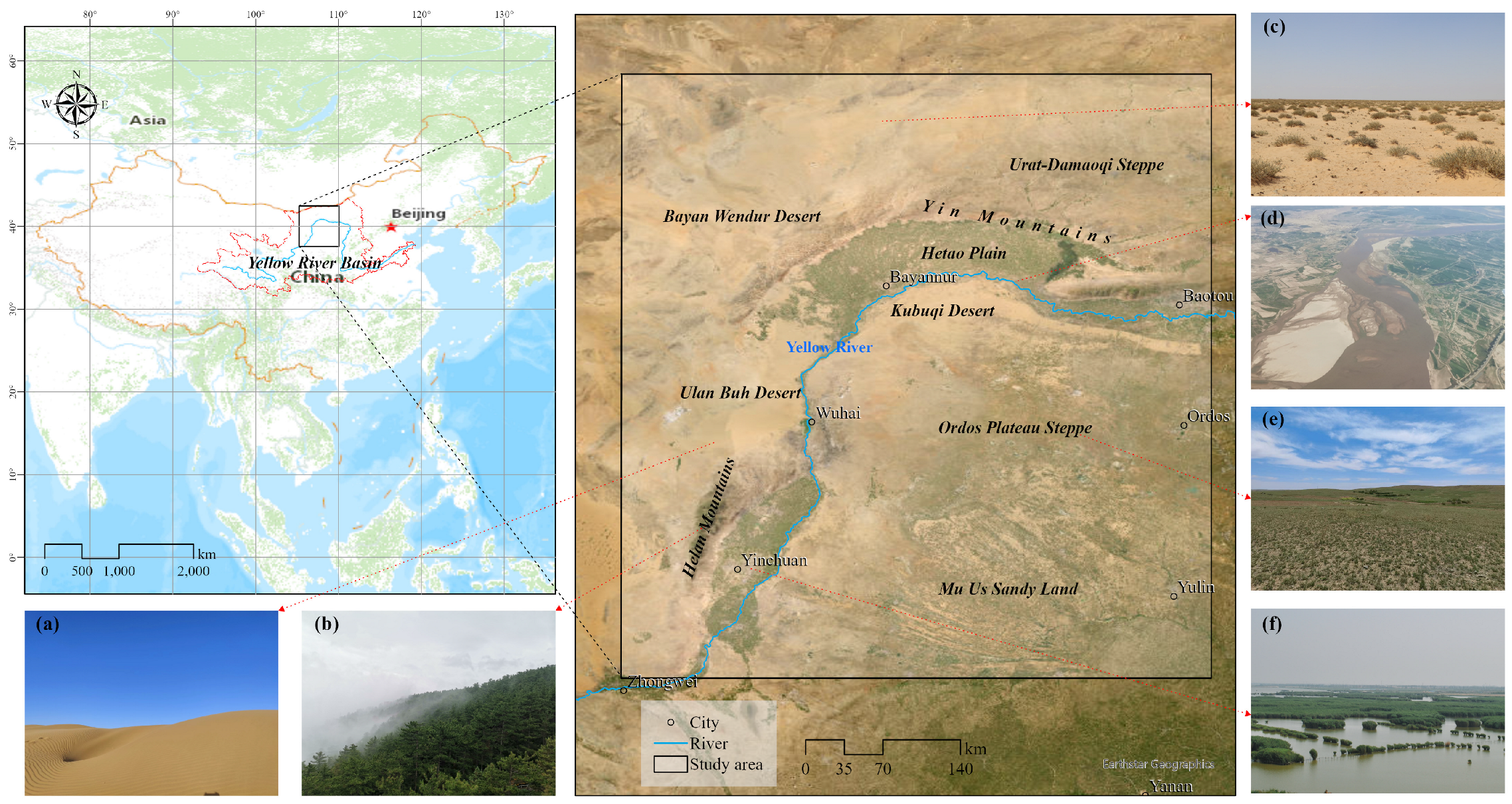
The study area located in the middle and upper reaches of the Yellow River Basin in northern China (37°33.98′–42°28.67′ N, 105°14.89′–110°25.64′ E), with a total area of 223,637.81 km2. The Yellow River crosses the study area (Figure 1). North of the river are Hetao Plain, Yin Mountains, Bayan Wendur Desert, and Gobi; to west of the river are Ulan Buh Desert, Yinchuan Plain, and Helan Mountains; to the south and east are Kubuqi Desert, Ordos Plateau Steppe, and Mu Us Sandy Land. The average annual precipitation ranges from 68 to 477 mm, the average annual temperature is from −1.9 °C to 9.6 °C, and the elevation varies from 806 to 3337 m above sea level. This area is characterized by an arid and windy climate, abundant sunshine, and high evaporation. The vegetation is dominated by desert, sandy land, Gobi, and steppe, with low biodiversity. The ecological environment is extremely fragile due to water scarcity, severe land desertification, soil degradation, and this area is prone to wind and water erosion. The population is primarily concentrated in the plains, with agriculture (wheat, corn) and animal husbandry (sheep) as the main economic activities. The industrial level is relatively low, mainly focused on resource extraction and primary processing.

Figure 1.
Location of the study area. (a): barren, (b): forest, (c): shrub-steppe, (d): water and cropland, (e): steppe, (f): wetland.
2.2. Data and Preprocessing
2.2.1. Satellite Data
Landsat 8 Operational Land Imager (OLI) surface reflectance images with 30 m spatial resolution were used as the primary data source for ecosystem classification. All surface reflectance images from the Landsat 8 OLI sensor covering the study area from 1 April to 30 September in 2022, which corresponds to the vegetation growing season in the study area, was acquired within the GEE [28]. The preprocessing of the Landsat 8 OLI imagery included cloud and cloud shadow contamination masking using the quality bands, followed by compositing using a median reducer, which uses the more frequent pixel value in the image stack to reduce the impact of atmospheric effects and cloud contamination [28,29].
The annual mosaics of ALOS-2 PALSAR-2 L-band data, which are seamless global SAR images created by mosaicking strips of PALSAR-2 SAR imagery, available in the GEE data catalog, were used as radar data [30]. Each mosaic contains a co-polarized HH backscatter (HH) and a cross-polarized HV backscatter (HV), both with a spatial resolution of 25 m [31]. The HH and HV were resampled to 30 m resolution to maintain consistency with the Landsat 8 data in the GEE.
The Shuttle Radar Topography Mission (SRTM) digital elevation model [32] with a spatial resolution of 30 m in the GEE data catalog was used to extract terrain data.
2.2.2. Sample Dataset
In this study, field survey samples were collected in August and September 2022, and supplementary field surveys were conducted during July and September 2023. To produce sufficient samples, high-resolution Google Earth imagery was also used along with the field data to produce the classification sample dataset [33]. Due to the high spatial heterogeneity within the study area, the sample selection process ensured a uniform distribution and a relatively balanced number of samples across all types. A total of 11,004 samples were obtained (Table 1), which were randomly partitioned into two subsets, with 70% of the samples used for training and the remaining 30% for validation [34].

Table 1.
Training and validation sample points in this study.
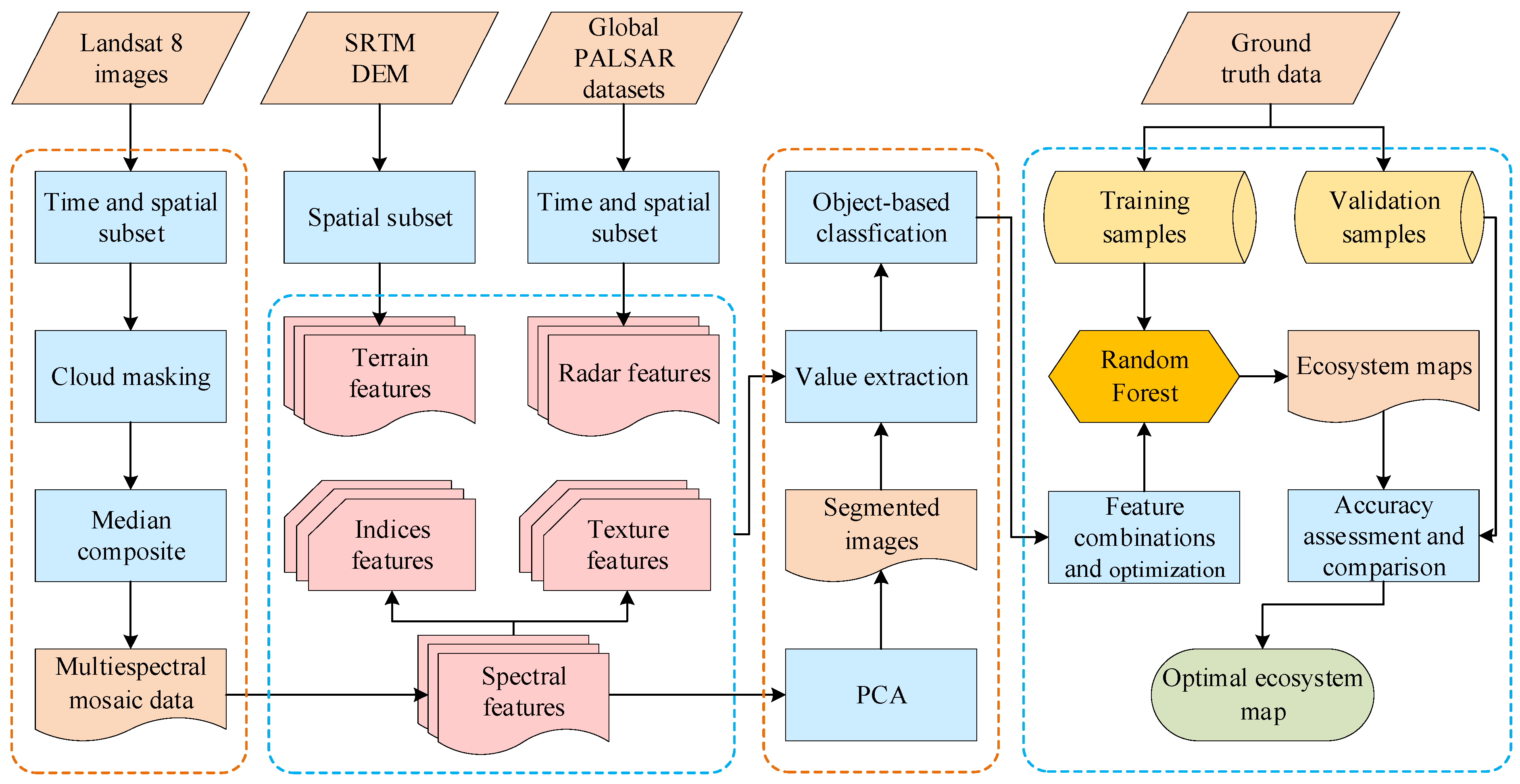
2.3. Technical Workflow
This study employs the GEE platform to map dryland ecosystems. The technical workflow employed in this study is illustrated in Figure 2. The main classification process comprises the following steps: Landsat 8 image preprocessing, selection of training and validation samples, construction of classification features, image segmentation, ecosystem classification, optimization of classification features, and accuracy assessment.
Figure 2.
Technical framework.
2.4. Classification System
Based on the existing remote-sensing-based ecosystem classification system [13], in conjunction with land cover and habitat type classifications from relevant studies [35,36,37,38,39], and considering the specific conditions of the study area, the ecosystems were categorized as follows: forest (including deciduous, evergreen, mixed, and sparse forest), shrub-steppe (the most distinctive dryland ecosystem, mainly sparse shrubs and mixed shrub-steppe with a small proportion of deciduous shrub, evergreen shrub), steppe (encompassing natural and semi-natural herbaceous steppe), cropland (including both irrigated and rainfed agricultural land), water (encompassing open water bodies such as rivers, lakes, ponds, and reservoirs), wetland (including wetland vegetation and lake marshes), built-up land (comprising urban and rural settlements, as well as infrastructure such as solar power plants, transportation networks, and industrial facilities), and barren (characterized by unvegetated land, including bare soils, salt flats, sandy fields, beaches, and bare exposed rock).
2.5. Ecosystem Classification in GEE
2.5.1. Feature Construction
A total of 24 classified features, including Landsat 8 spectral bands, spectral indices, terrain features, radar features, and texture features, were selected to construct the feature dataset for mapping ecosystems in the study area (Table 2). All features were obtained and calculated in the GEE.
Table 2.
Features of ecosystem classification in this study.
Landsat 8 OLI surface reflectance image contains 9 bands ranging from a wavelength of 0.433 to 2.3 µm. Based on the specific conditions of the study area, we excluded the coastal band used for coastal zone observations, the pan band for enhanced resolution, and the cirrus band for cloud detection. The blue, green, red, near-infrared (nir), shortwave infrared 1 (swir1), and shortwave infrared 2 (swir2) bands from the median image were selected as spectral features.
Based on the ecosystem types in this study, we selected the following spectral indices: Normalized Difference Vegetation Index (NDVI) [40], Enhanced Vegetation Index (EVI) [41,42], Modified Soil Adjusted Vegetation Index (MSAVI) [43], Spectral Variability Vegetation Index (SVVI) [44], Normalized Difference Built-Up Index (NDBI) [45], Modified Normalized Difference Water Index (MNDWI) [46], Wet Index (WET) [47,48] and Salinity index (SIT) [49,50]. The calculation formulae and significance for these indices are shown in Table 3.
Terrain features play a crucial role in shaping the spatial heterogeneity of dryland ecosystems. Elevation and slope were extracted using SRTM digital elevation model as essential terrain features in this study. Radar can obtain object roughness, texture, and other information unrestricted by weather and lighting conditions. When combined with optical remote sensing data, it can better explain, enhance, and analyze various surface features [51]. The HH and HV were selected as radar features to distinguish dryland ecosystems.
Texture features are helpful for image classification [52]. We generated a gray level image by a linear synthesis method for nir, red, and green bands (Equation (1)), and extracted texture features using gray level co-occurrence matrix (GLCM) [53], which can reflect the degree of uniformity of gray level distribution and texture thickness of the image [54]. Drawing upon relevant studies [9,55,56,57,58,59,60], we ultimately selected six GLCM metrics: angular second moment (gray_asm), correlation (gray_corr), variance (gray_var), inverse difference moment (gray_idm), and dissimilarity (gray_diss) as texture features incorporated in the classification process.
where nir, red, and green correspond to the respective bands of Landsat 8.
Table 3.
The formulae of spectral indices used in this study.
Table 3.
The formulae of spectral indices used in this study.
| Indices | Formula | Description |
|---|---|---|
| NDVI | NDVI is the most widely used vegetation index for effectively discriminating vegetation from water and soil. It proves useful for monitoring vegetation growth status, quantifying vegetation cover, and mitigating partial radiometric errors [54]. | |
| EVI | EVI can enhance the physiological, biochemical, and structural characteristics of the vegetation canopy and is helpful in mitigating the saturation effects observed in NDVI over areas of high vegetation cover [61]. | |
| MSAVI | MSAVI reduces soil background interference in sparsely vegetated regions, thereby facilitating vegetation extraction. | |
| SVVI | SVVI are employed to discriminate between forest, steppe, and cropland classes that would otherwise be challenging to differentiate spectrally [44]. | |
| NDBI | NDBI aids in the extraction of urban, industrial, mining, and residential construction land [54]. | |
| MNDWI | MNDWI is used for water body extraction and can easily distinguish shadows from water bodies, addressing the issue of shadow removal in water body extraction [62]. | |
| SIT | Certain regions within the study area suffer from severe salinization. SIT facilitates the extraction of highly saline lands. | |
| WET | WET can effectively reflect the moisture conditions of surface vegetation and soil [63]. |
Note: nir, red, blue, green, swir1, swir2 in formula correspond to the respective bands of Landsat 8 OLI images.
2.5.2. Image Segmentation
Unlike most studies that employ pixel-based methods for classification, we adopted an object-based approach for classification within the GEE. The object-based approach can integrate multiple classification features to enhance the identification ability in heterogeneous areas, and can produce classification results with good spatial consistency and continuity, effectively mitigating salt and pepper noise [64].
Image segmentation was performed using the Simple Non-Iterative Clustering (SNIC) algorithm within the GEE. To obtain optimal segmentation results, principal component analysis (PCA) was applied to the blue, green, red, nir, swir1, and swir2 bands. Subsequently, the input images required for SNIC were selected based on the principal component contribution rates. In this study, the top three principal components, accounting for a cumulative contribution rate of 99.25%, were selected as inputs to the SNIC algorithm. This contribution rate is sufficient to effectively characterize the spectral information of the image. Moreover, by utilizing the top three principal components and the robust SNIC algorithm, the impacts of noise in the principal component analysis were greatly mitigated.
2.5.3. RF Classification
The GEE provides a suite of commonly used machine learning algorithms. Among these algorithms, RF has proven to be the most effective and widely applicable for land use, habitat, or ecosystem mapping applications [57,65,66,67]. RF algorithm is an ensemble learning method that constructs multiple decision trees during training and outputs the class that is the mode of the predictions from individual trees. It offers several advantages, including the ability to handle high dimensional data, robustness to noise and outliers, and estimation of feature importance in the classification process. For this study, an RF algorithm was selected to categorize and map ecosystems due to its proven performance and versatility.
2.6. Feature Combination and Optimization
To achieve optimal classification accuracy, feature selection was conducted from two perspectives: combining classification features and optimizing feature selection. Initially, five feature combinations were established by integrating spectral bands, spectral indices, terrain features, radar features, and texture features (Table 4). The accuracy of these different feature categories was then evaluated. Subsequently, within the optimal feature combination, the classification features were ranked based on their relative importance. Features were incrementally added to the classification model based on their importance ranking, and the effect of incorporating an increasing number of features on classification accuracy was evaluated, thereby optimizing the set of features included in the final classification model [34].
Table 4.
Classification feature categories of different combinations.
2.7. Accuracy Assessment
Accuracy assessment is an important component in evaluating the reliability of classification results [68]. Using validation samples (Table 1) and a confusion matrix, multiple metrics were selected to assess the classification accuracy of ecosystems in the study area: overall accuracy (OA), kappa coefficient (KC), user’s accuracy (UA), and producer’s accuracy (PA). OA reflects the proportion of correctly classified samples in the study area. KC indicates the degree of consistency between the actual ecosystems and the predicted types. UA represents the proportion of a given ecosystem type that is correctly predicted. PA is the proportion of a given ecosystem type that is correctly identified [59].
While KC has faced criticism [69,70], it was still included in this study due to its provision of a standardized similarity measure, which allows for easy cross-study comparison and straightforward evaluation of relative classification performance, especially when comparing various classifications with randomized samples. However, it is essential to recognize the limitations of KC and not overly rely on it as the sole validation metric [71].
3. Results
3.1. Accuracy Comparison under Different Combinations
The classification accuracies of the five feature combinations are presented in Table 5. Combination C5, which integrated spectral bands, spectral indices, terrain features, radar features, and texture features, achieved the highest accuracy (OA: 90.76%; KC: 0.89). In contrast, combination C1, utilizing only spectral bands and spectral indices, exhibited the lowest classification accuracy (OA: 80.16%; KC: 0.77). Compared with C1 as the baseline, the individual addition of terrain (C2), radar (C3), and texture features (C4) led to improvements in both OA and KC for ecosystem classification in the study area. The greatest improvement was observed for C3, followed by C2, then C4, with OA increasing by 4.04%, 6.54%, and 2.37%, respectively, and KC increasing by 0.05, 0.07, and 0.03, respectively, relative to C1. These results indicate that, in the context of dryland ecosystems classification, the contribution of the three feature types to classification accuracy is in the following order: radar features > terrain features > texture features.
Table 5.
Accuracy assessment of different feature combinations.
As shown in Table 5, the contributions of terrain, radar, and texture features to the classification accuracies varied considerably across different ecosystems in the study area. For cropland and water, the C1 combination achieved relatively high UA values of 90.87% and 94.25%, respectively. The addition of terrain, radar, and texture features had minimal impact on the classification accuracy of these two ecosystems. Specifically, for water, the inclusion of terrain and radar features marginally improved the UA by 1.5% and 1%, respectively, while the addition of texture features led to a slight decline of 1%. Regarding cropland, the incorporation of texture features resulted in a 1.37% increase in UA, whereas terrain features had no influence, and radar features led to a 1.37% decrease.
Regarding built-up land, the C1 combination achieved a UA of 86.48%. The incorporation of terrain features slightly improved UA, while the inclusion of radar features further increased it to 92.7%. However, the addition of texture features led to a decline in UA. For forest and shrub-steppe, the inclusion of terrain, radar, and texture features resulted in UA improvements, with radar features contributing the most substantial increase, followed by terrain features, and texture features contributing the least. The magnitude of improvement differed significantly between radar and texture features, with differences in the increase reaching 8.31% and 8.68% for the two ecosystems, respectively. As for steppe, wetland, and barren, the addition of terrain, radar, and texture features individually enhanced UA. However, radar features contributed the most considerable increase for steppe (12.47%), terrain features for wetland (6.48%), and texture features for barren (8.01%).
When all classification features were incorporated, UA attained its highest levels for all ecosystems (except cropland), reaching 94.18% for forest, 86.60% for shrub-steppe, 84.71% for steppe, 95.50% for water, 87.05% for wetland, 94.21% for built-up land, and 90.08% for barren.
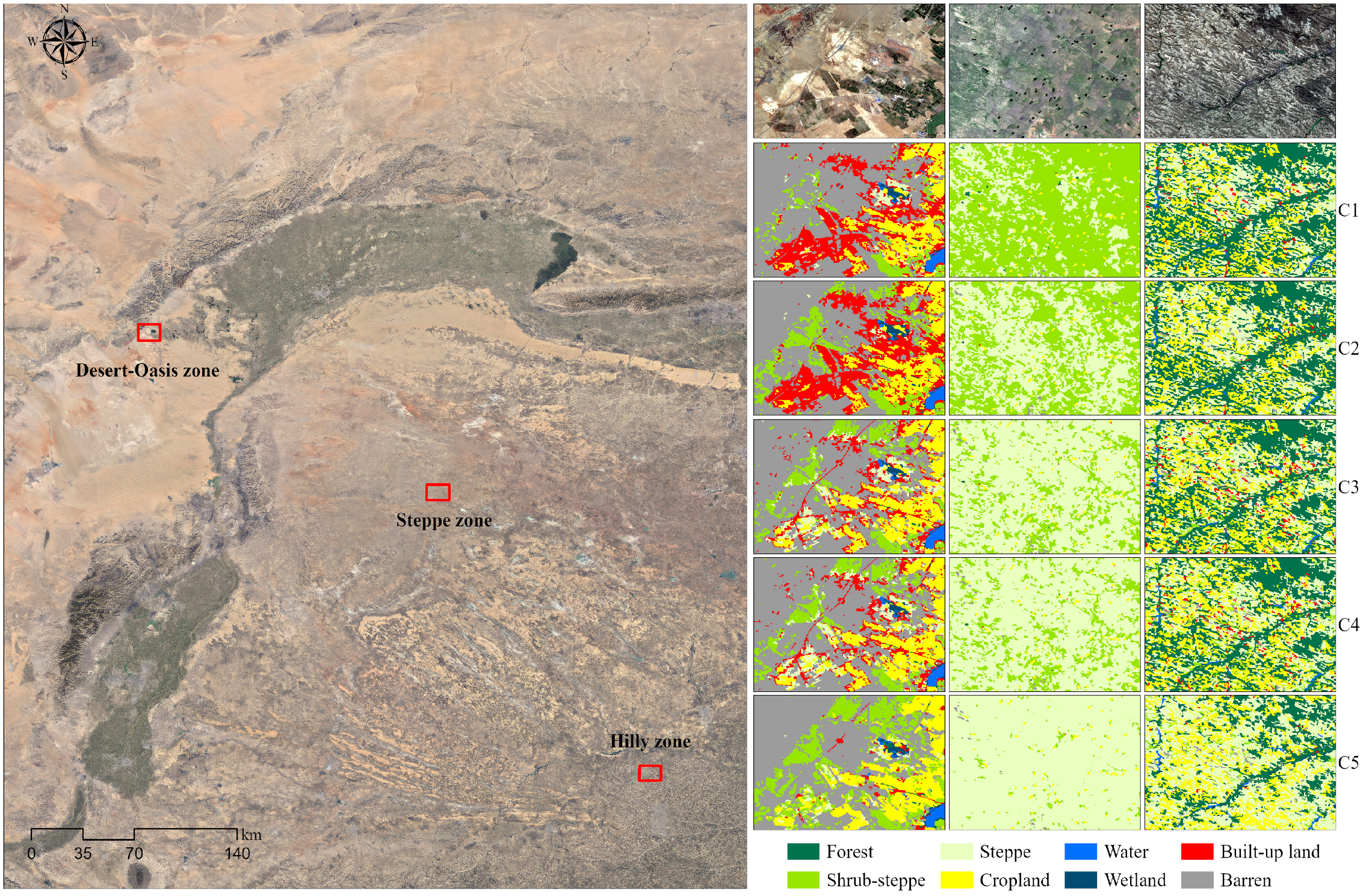
Figure 3 illustrates the variations in the spatial distribution accuracy of ecosystems across different classification combinations. C1, C2, C3, and C4 misclassified certain barren areas, such as salt flats, beaches, and bare exposed rock, as well as transition zones between ecosystems, as built-up land. Moreover, a substantial portion of steppe within the Ordos Plateau region was erroneously classified as shrub-steppe, leading to an overestimation of the shrub-steppe extent and area. Although C1 or combinations with a single additional feature dataset (C2, C3, and C4) could delineate the forest distribution relatively well, misclassifications occurred in the southeastern loess hilly zone, where steppe and cropland were incorrectly labeled as forest, resulting in an overestimation of the forest area. Consequently, in practical classification endeavors, it is crucial not only to evaluate classification accuracy using quantitative metrics such as OA, KC, UA, and PA, but also to incorporate field observations and local knowledge of the study area to accurately delineate ecosystems. This integrated approach ensures that the classified map accurately represents the spatial distribution and extent of ecosystems on the ground.

Figure 3.
Visual comparison of different feature combinations in three typical zones.
3.2. Feature Importance and Optimization
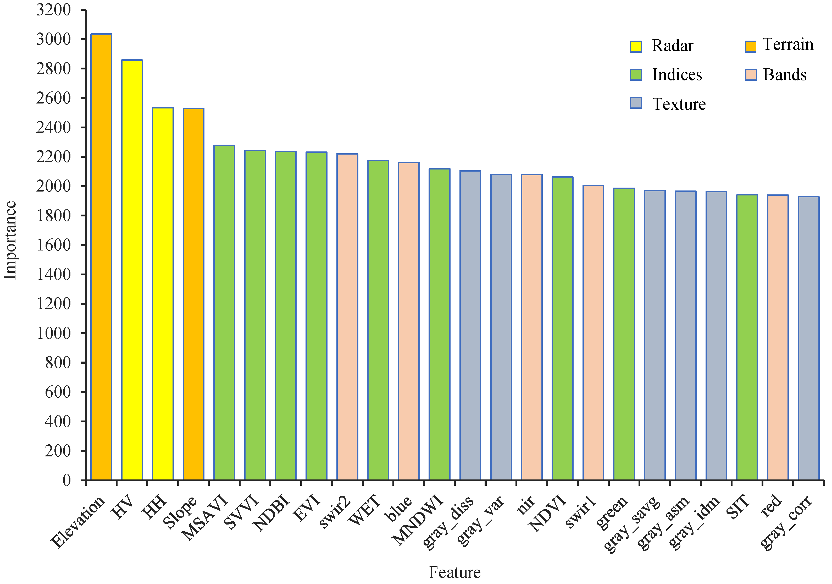
During the classification process, the average importance scores of various features were plotted using the feature importance ranking function embedded in the GEE (Figure 4). It is evident that the terrain and radar features had the highest importance scores, indicating their most significant contributions to the classification of ecosystems in the study area. Firstly, the importance score of elevation (3033.87), HV (2858.14), HH (2534.49), and slope (2528.64) were significantly higher than those of other features. Secondly, spectral index features such as MSAVI, SVVI, NDBI, and EVI had comparable importance scores, closely following terrain and radar features, while the importance scores of the remaining spectral indices were relatively scattered. The contributions of spectral band feature variables to ecosystem classification varied, and their importance rankings were relatively dispersed. Finally, for texture features, the highest ranked gray_diss was only ranked 13th, while the lowest ranked gray_corr had an importance score of 1928.71. Although the five categories of features showed overall differences in importance, the importance scores of spectral indices, spectral bands, and texture features were relatively balanced with minor differences. This indicates that under the complex natural geographic conditions of the study area, the synergistic effects of multiple features are necessary to achieve satisfactory classification results. The integration of complementary information from various feature categories enhances the discriminative power of the classification model, ultimately improving the accuracy of ecosystems mapping.

Figure 4.
Importance of features for the RF algorithm.
To further improve classification accuracy, we explored the changes in accuracy by incrementally adding features according to their importance ranking, with the results shown in Figure 5. A rapid improvement in classification accuracy was observed as the number of features increased from 3 to 5, mainly due to the high importance scores of the initially added features. As more features were progressively included, the classification accuracy exhibited a fluctuating upward trend. When the number of features reached 13, OA and KC for the study area reached 91.07% and 0.90, respectively, indicating a relatively high accuracy in delineating ecosystems. As the number of features continued to increase beyond 13, OA and KC showed a very gradual fluctuating increase, reaching their highest values of 91.34% and 0.90, respectively, when 19 features were included. Subsequently, the classification accuracy decreased as more features were added, with OA registering 90.89% and KC at 0.89 when the feature reached its maximum of 24. This decrease in accuracy can be attributed to the increased model complexity and overfitting caused by the addition of redundant features [72]. Therefore, we selected the top 19 ranked features based on their importance scores for mapping ecosystems in the dryland region, as this configuration achieved the highest accuracy while avoiding potential overfitting issues.
Figure 5.
Variation of classification accuracy with different number of features.
3.3. Accuracy Assessment of Optimal Feature Dataset
Utilizing the optimized set of 19 classification features for ecosystem mapping, OA and KC achieved 91.34% and 0.90, respectively, indicating a relatively high level of accuracy for the study area. The classification accuracies for different ecosystems are also presented in Table 6. PA for forest, cropland, water, wetland, built-up land, and barren classes were all above 90%, with built-up land reaching 96.29%. PA for shrub-steppe and steppe were slightly lower at 89.03% and 84.36%, respectively. Regarding UA, forest, cropland, water, wetland, and built-up land all exceeded 90%, while shrub-steppe, steppe, and barren exhibited UA values above 85%. These OA, KC, PA, and UA indicate that utilizing the optimized set of 19 classification features achieved a relatively high classification accuracy for mapping ecosystems in this study area, enabling the characterization of the current ecosystem status.
Table 6.
Confusion matrix of the optimal classification.
3.4. Classification Result
Utilizing the GEE, we implemented object-based image segmentation on the Landsat 8 OLI multispectral imagery using the SNIC algorithm. Subsequently, we optimized the final feature set employed for the random forest classification by evaluating the effects of different feature combinations and incrementally increasing the number of features. Utilizing this optimized feature set as input data and the test samples from the classification samples for model training, the ecosystem map for the study area was produced (Figure 6 and Table 7).
Figure 6.
Spatial representation of the optimal classification in 2022.
Table 7.
Area and percentage of each ecosystem in 2022.
An examination of the classification results reveals that steppe and barren are the most extensive ecosystems, accounting for 29.87% and 29.19% of the total area, respectively. Steppe is contiguous distributed in western Ordos, the Urat-Damaoqi region north of the Yin Mountains, with smaller patches in the western foothills of the Helan Mountains. It is interspersed with barren and forest areas in the Mu Us Sandy Land and the loess hilly regions in the southeastern part of the study area. Barren is primarily located within the Yin-Helan Mountains Range, several deserts and Gobi regions west of the Yin Mountains, the Ulan Buh Desert, the Kubuqi Desert, and the Mu Us Sandy Land. Shrub-steppe, another predominant ecosystem occupying 22.18% of the total area, is predominantly distributed in desert, sandy land, and Gobi regions, with scattered occurrences in steppe areas. Cropland, occupying 10.46% of the area, is mainly concentrated in the Hetao Plain and Yinchuan Plain, which are among the major agricultural regions in northern China, and is also widely distributed in steppe areas, the Mu Us Sandy Land, and the loess hilly regions. Forest accounts for 4.52% of the total area and is primarily found in the Helan Mountains, Wula Mountain, the vicinity of Ordos City, and the southeastern loess hilly region of the study area.
4. Discussion
4.1. Comparison of Classification Algorithms
In this study, we employed an RF algorithm to map dryland ecosystems of an ecologically critical area in northern China. Prior to this, we compared the suitability of three commonly used algorithms—RF, CART, and SVM—to determine the most appropriate classification algorithm.
Previous studies have consistently demonstrated the superior performance of RF in various aspects of dryland research. For instance, Tian et al. [73] compared the effectiveness of RF, SVM, and ANN in classifying wetland types in the arid regions of Xinjiang and found that RF had 10% higher classification accuracy than the other two algorithms. Wu et al. [74] used RF to estimate evapotranspiration in an arid oasis region in northwestern China, achieving excellent results. Similarly, Lu et al. [60] found that RF had a significant advantage in extracting desert information in the alpine arid regions of Qinghai, China. The advantages of RF have also been demonstrated in many studies focusing specifically on land cover mapping in arid regions [9,62,75].
Different algorithms have their inherent strengths and weaknesses, which has led to numerous studies investigating the effectiveness of different machine learning methods in different contexts. For example, Mustak et al. [76] found that SVM outperformed RF in terms of classification effectiveness for crop classification. Therefore, it is still necessary to compare the application effects of different machine learning algorithms before undertaking ecosystem mapping to ensure optimal classification results.
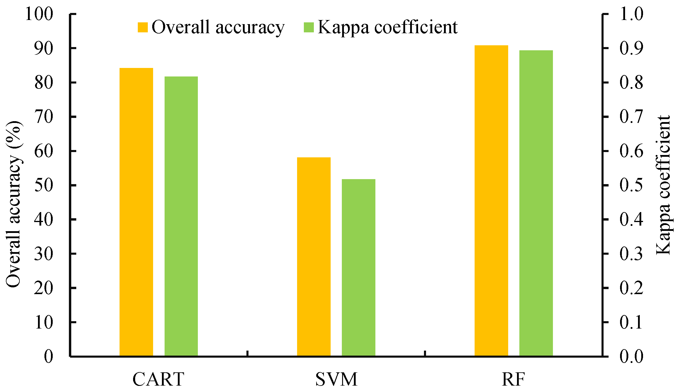
The results, as shown in Figure 7, reveal that RF achieved the highest OA of over 90% and a KC above 0.9. CART followed with an OA of 84.20% and a KC of 0.82, while the SVM algorithm performed the poorest with an OA of only 58.04% and a KC of 0.52. Both CART and SVM failed to meet the requirements for accurate ecosystem mapping in the study area. These results indicate that RF is the most suitable classification approach for ecosystem mapping in the study area.
Figure 7.
Comparison of the accuracy of three machine learning algorithms.
The superior accuracy of RF over CART in this study can be attributed to its ensemble nature, which mitigates overfitting by aggregating multiple decision trees [34]. This advantage makes RF particularly suitable for complex classification tasks in heterogeneous environments. In addition, the ability of RF to handle high-dimensional data and its robustness to noise and outliers also contribute to its superior performance. In contrast, CART is more susceptible to accuracy reductions due to excessive features [60], and SVM, despite its effectiveness in certain scenarios [76], faced challenges in accurately classifying the complex and heterogeneous nature of dryland ecosystems in this study.
4.2. The Impacts of Classification Features to Ecosystems Mapping
Given the spectral heterogeneity within the same ecosystem and the spectral homogeneity among different types, relying solely on spectral bands poses challenges for complex ecosystem classification [77]. To ensure classification accuracy, this study comprehensively considered spectral bands, spectral indices, terrain, radar, and texture features. Firstly, a series of spectral indices, including vegetation indices, built-up indices, salinity indices, water indices, and spectral variation indices, were used to support the classification process. Secondly, the distribution of ecosystems is directly or indirectly influenced by topography and geomorphology [78], necessitating the inclusion of terrain features in the classification framework. Furthermore, due to the unique characteristics of dryland environments, such as low vegetation cover and soil background interference, the discrimination of shrub-steppe, barren, and steppe ecosystems may not be effectively achieved based on spectral or terrain features alone. Therefore, texture and radar features were incorporated into the classification framework.
We found that the combination of different feature categories affected the classification accuracy of different ecosystems in different ways. The inclusion of radar features (Combination C3) significantly improved classification accuracy for forest, shrub-steppe, steppe, and built-up land by 10.53%, 9.67%, 12.47%, and 6.22%, respectively, compared to C1. This improvement is attributed to radar’s ability to provide information on surface roughness and moisture content [79,80], which helps distinguish these ecosystems with different structural and moisture characteristics. Terrain features had the most substantial impact on the classification accuracy of water and wetland (1.5% and 6.48%, respectively, compared to C1), as these ecosystems are often associated with specific topographic conditions. Texture features improved the classification of cropland and barren (1.37% and 8.01%, respectively, compared to C1) because the spatial arrangement of pixel values captured by texture features helps to differentiate these ecosystems [53], particularly where cropland has regular planting patterns and barren land has uniform surface characteristics. However, the combination incorporating all classification feature categories yielded the best classification results for most ecosystems, reflecting the potential complexity of ecosystem classification in the study area and the need for multiple features to work together for optimal performance. Simultaneously, this highlights the importance of integrating multi-source data (e.g., spectral imagery and synthetic aperture radar imagery) to overcome the limitations of individual data sources and improve classification accuracy.
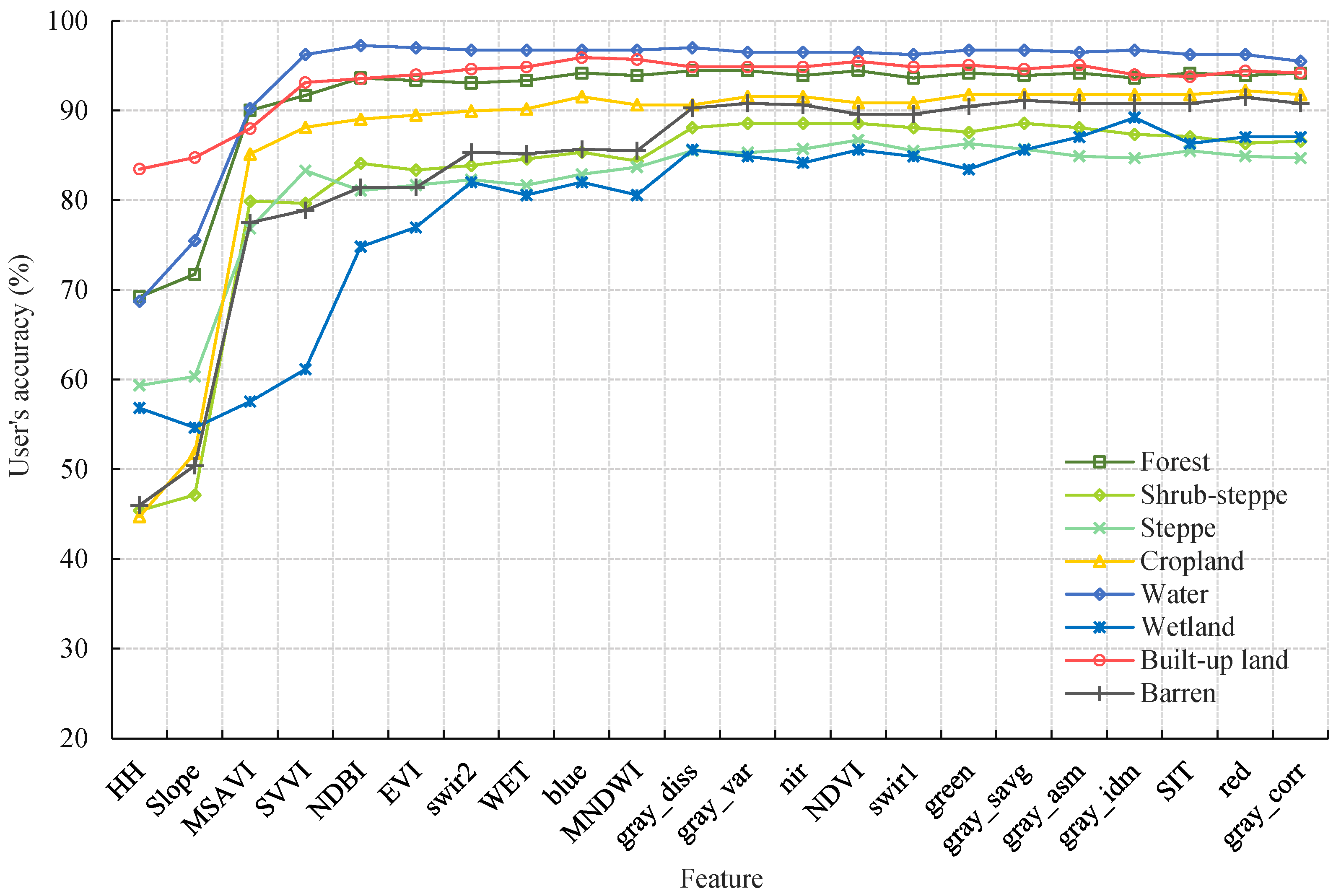
Of course, an excessive number of classification features does not necessarily lead to better results, as redundant information can reduce classification accuracy [72]. Our results, obtained by incrementally adding features, indicate that there are redundant features among the 24 classification features that we selected in this study. As shown in Figure 5 and Figure 8, the addition of gray_asm, gray_idm, SIT, red, and gray_corr resulted in a decrease in classification accuracy for entire as well as for individual ecosystems such as shrub-steppe, steppe, wetland, and built-up land. These results are consistent with those of several other feature optimization studies [34,72,81]. Therefore, optimizing classification features when there are too many becomes particularly important.
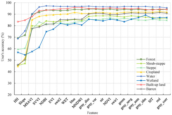
Figure 8.
Variation of user’s accuracy with the number of features for each ecosystem.
Screening for redundant classification features based on the overall increase or decrease in classification accuracy is a commonly used method, but evaluating features by considering the classification accuracy of individual ecosystems has not yet been studied. In this study, the changes in UA for different ecosystems after incorporating various classification features are shown in Figure 8. Classification features have different effects on different ecosystems. For example, the initial addition of the slope feature resulted in a 2.16% decrease in UA for wetland, while other types improved by 1.01% to 6.75%. The optimal UA for forest, shrub-steppe, steppe, cropland, water, wetland, built-up land, and barren in the study area were achieved after incorporating the gray_diss, gray_var, NDVI, red, NDBI, gray_idm, blue, and red features, respectively. These results indicate that the appropriate combination of features should be selected based on the specific research objectives and classification goals.
4.3. Mapping Ecosystems in Dryland Regions
In this study, GEE and the RF algorithm were employed to map dryland ecosystems and achieving satisfactory classification results (OA: 91.34%; KC: 0.90). PA and UA of forest (including sparse forest), shrub-steppe (including sparse shrub and mixed shrub-steppe), and barren all achieved relatively high accuracy (93.91%, 88.59%, and 85.61%, respectively), demonstrating the feasibility and effectiveness of extracting sparse vegetation ecosystems in dryland regions.
It is worth noting that there were only a few validation samples where forest was misclassified as shrub-steppe, steppe, or barren (as shown in Table 6). This indicated that forest can be effectively separated from barren, and forest can be accurately distinguished from shrub-steppe and steppe in this study. Additionally, shrub-steppe was distinguished from barren. Compared to traditional ecosystem classification methods or remote-sensing-based approaches that mainly rely on modifying land use data in this study area [14,82,83], the method we used can correctly identify sparse forest as forest and capture sparse shrub. For example, We et al. [83] identified only 0.92% and 2.05% of the area as forest and shrubland, respectively, based on GlobeLand30 data for regions that significantly overlap with our study. This discrepancy is partly due to our inclusion of sparse forest and shrub under different definitions. However, it also highlights that overlooking such sparse vegetation in land use or ecosystem studies can lead to a substantial underestimation of their ecological significance in the region.
While satisfactory classification results have been achieved for both ecosystems as a whole and individually in this study, there is still some misclassification for certain ecosystems (as shown in Table 6). The main misclassification cases involved shrub-steppe and steppe, steppe and cropland, and steppe and wetland. Specifically, the misclassification between shrub-steppe and steppe in this study can be attributed to the natural shrub-steppe structure formed by steppe degradation [84,85] and the artificially planted shrub on steppe, both of which retain a steppe background and share similar ecological and visual characteristics, including some common herbaceous vegetation types [9,28]. Additionally, in some areas, the similar graminoid vegetation and moisture conditions present in steppe, cropland, and wetland ecosystems have led to misclassification among these ecosystems. All these misclassifications can be attributed to the similarities in spectral, textural, and topographical among these ecosystems, which are challenging to distinguish using commonly used remote sensing data [86]. To address these misclassifications, some studies focusing on land and vegetation classification have attempted to conduct classification studies from different perspectives of vegetation phenology [9,87]. This approach could be an important direction for future research, as it could improve the accuracy of distinguishing ecosystems with similar characteristics.
Overall, the satisfactory classification results achieved in this study can be attributed to the following reasons. Firstly, the integration and use of multi-source remote sensing data in GEE allows the unique features of these sparse vegetation ecosystems to be characterized from multiple perspectives, including spectral, surface roughness, texture, and topography. Secondly, feature combination and optimization were conducted to eliminate redundant features and avoid a decrease in classification accuracy. Thirdly, the advantages of the RF algorithm, which can integrate various features through ensemble learning, enabled accurate ecosystems mapping. Additionally, this method can be used for the time-series mapping of dryland ecosystems, providing a reference for further in-depth investigations of their structure, function, and services. This will support ecosystem restoration, enhance ecosystem resilience and recovery capacity, and ultimately maintain ecological balance and sustainable development in this area.
4.4. Limitations and Future Perspectives
While GEE and the RF algorithm proved efficient for ecosystem classification in dryland regions, several methodological limitations were identified in this study. Firstly, the optimization of the classification feature set was based on incrementally adding features according to their importance ranking, without adequately considering collinearity among indicators. Future research should address this issue by further optimizing the feature selection method to account for potential collinearity and redundancy. Additionally, the classification features in this study were derived solely from GEE integrations or calculations, lacking external data such as soil data, which can directly influence ecosystem characteristics. Incorporating more diverse and representative external datasets, including soil and climatic data, could further enhance classification accuracy. The study was also limited by the resolution and availability of the remote sensing data used. While Landsat 8 provided valuable information, more spectrally advantageous Landsat 9 and higher-resolution Sentinel-2 data could offer more detailed insights and potentially improve classification accuracy. Future research should explore these datasets to improve the accuracy of dryland ecosystems mapping. Moreover, this study focused on a specific timeframe, neglecting the dynamic nature of ecosystems, which are subject to temporal changes. Incorporating time-series analysis and exploring the temporal dynamics of ecosystems would provide a more comprehensive understanding of ecosystem changes over time.
Overall, this study presents a systematic methodological integration for mapping typical dryland ecosystems with satisfactory classification results. Future research should focus on improving classification accuracy by incorporating diverse datasets, addressing feature collinearity, further subdividing ecosystem types, and exploring the application of the latest remote sensing technologies and advanced machine learning algorithms. These efforts will enhance ecosystem mapping capabilities and support the better management and conservation of drylands.
5. Conclusions
This study aimed to explore accurate mapping of ecosystems in a typical dryland region by integrating Google Earth Engine (GEE), the random forest (RF) algorithm, multi-source remote sensing data, feature optimization, and image segmentation techniques. The main conclusions are as follows: (1) integrating the GEE and RF algorithm proved effective for dryland ecosystem mapping, achieving an OA of 91.34% and a KC of 0.90. (2) The mapping accuracy exceeded 90% for ecosystems such as forest, cropland, built-up land, and water, while for widespread sparse vegetation ecosystems like shrub-steppe, the accuracy was slightly lower but still above 85%, demonstrating the efficacy of this approach for mapping sparse dryland vegetation. (3) The classification accuracy of dryland ecosystem mapping was significantly improved through the combination and optimization of features from multi-source remote sensing data, including spectral, terrain, radar, and texture features, compared to using spectral data alone. Among these, radar features contributed the most to improving accuracy, followed by terrain and texture features. (4) The study accurately mapped and characterized the major dryland ecosystems, identifying steppe, barren, and shrub-steppe as the most widespread, with croplands concentrated along the Yellow River plains and forests in mountainous and loess hilly regions. (5) Accurate dryland ecosystem mapping requires considering regional spatial heterogeneity, selecting more suitable remote sensing data and classification features based on actual conditions. Future research should focus on feature selection methods, incorporating more diverse ancillary datasets, and exploring the potential of higher spatial and spectral resolution satellite imagery. This study provides a baseline ecosystem map and a methodological framework supporting ecological policies in the study area, while also serving as a reference for precise ecosystem mapping in other dryland regions worldwide.
Author Contributions
Conceptualization, S.L. and Q.L.; methodology, S.L.; formal analysis, S.L. and P.G.; investigation, S.L., P.G., F.S. and X.D.; visualization, S.L.; supervision, Q.L.; writing—original draft, S.L.; writing—review and editing, S.L., J.Z., X.C. and Q.L. All authors have read and agreed to the published version of the manuscript.
Funding
This research was funded by National Nonprofit Institute Research Grant of Chinese Academy of Forestry (grant number CAFYBB2021MC002-02), National Nonprofit Institute Research Grant of Chinese Academy of Forestry (grant number CAFYBB2021ZB003-04), and Science & Technology Fundamental Resources Investigation Program (grant number 2023FY100703).
Data Availability Statement
Primary data can be obtained from the GEE platform. Additionally, the original contributions presented in the study are included in the article; further inquiries can be directed to the corresponding author.
Conflicts of Interest
The authors declare no conflicts of interest.
References
- Schulze, J.; Frank, K.; Müller, B. Governmental Response to Climate Risk: Model-Based Assessment of Livestock Supplementation in Drylands. Land Use Policy 2016, 54, 47–57. [Google Scholar] [CrossRef]
- D’Odorico, P.; Bhattachan, A. Hydrologic Variability in Dryland Regions: Impacts on Ecosystem Dynamics and Food Security. Philos. Trans. R. Soc. Lond. B Biol. Sci. 2012, 367, 3145–3157. [Google Scholar] [CrossRef] [PubMed]
- Smith, W.K.; Dannenberg, M.P.; Yan, D.; Herrmann, S.; Barnes, M.L.; Barron-Gafford, G.A.; Biederman, J.A.; Ferrenberg, S.; Fox, A.M.; Hudson, A.; et al. Remote Sensing of Dryland Ecosystem Structure and Function: Progress, Challenges, and Opportunities. Remote Sens. Environ. 2019, 233, 111401. [Google Scholar] [CrossRef]
- Baka, J. Making Space for Energy: Wasteland Development, Enclosures, and Energy Dispossessions. Antipode 2017, 49, 977–996. [Google Scholar] [CrossRef]
- Madhusudan, M.D.; Vanak, A.T. Mapping the Distribution and Extent of India’s Semi-Arid Open Natural Ecosystems. J. Biogeogr. 2023, 50, 1377–1387. [Google Scholar] [CrossRef]
- Zeng, H.; Wu, B.; Zhang, M.; Zhang, N.; Elnashar, A.; Zhu, L.; Zhu, W.; Wu, F.; Yan, N.; Liu, W. Dryland Ecosystem Dynamic Change and Its Drivers in Mediterranean Region. Curr. Opin. Environ. Sustain. 2021, 48, 59–67. [Google Scholar] [CrossRef]
- Naidoo, R.; Hill, K. Emergence of Indigenous Vegetation Classifications through Integration of Traditional Ecological Knowledge and Remote Sensing Analyses. Environ. Manag. 2006, 38, 377–387. [Google Scholar] [CrossRef] [PubMed]
- Meng, B.; Zhang, Y.; Yang, Z.; Lv, Y.; Chen, J.; Li, M.; Sun, Y.; Zhang, H.; Yu, H.; Zhang, J.; et al. Mapping Grassland Classes Using Unmanned Aerial Vehicle and MODIS NDVI Data for Temperate Grassland in Inner Mongolia, China. Remote Sens. 2022, 14, 2094. [Google Scholar] [CrossRef]
- Shafizadeh-Moghadam, H.; Khazaei, M.; Alavipanah, S.K.; Weng, Q. Google Earth Engine for Large-Scale Land Use and Land Cover Mapping: An Object-Based Classification Approach Using Spectral, Textural and Topographical Factors. GISci. Remote Sens. 2021, 58, 914–928. [Google Scholar] [CrossRef]
- Crossman, N.D.; Burkhard, B.; Nedkov, S.; Willemen, L.; Petz, K.; Palomo, I.; Drakou, E.G.; Martín-Lopez, B.; McPhearson, T.; Boyanova, K.; et al. A Blueprint for Mapping and Modelling Ecosystem Services. Ecosyst. Serv. 2013, 4, 4–14. [Google Scholar] [CrossRef]
- Blasi, C.; Capotorti, G.; Alós Ortí, M.M.; Anzellotti, I.; Attorre, F.; Azzella, M.M.; Carli, E.; Copiz, R.; Garfì, V.; Manes, F.; et al. Ecosystem Mapping for the Implementation of the European Biodiversity Strategy at the National Level: The Case of Italy. Environ. Sci. Policy 2017, 78, 173–184. [Google Scholar] [CrossRef]
- Lei, G.; Li, A.; Tan, J.; Bian, J.; Zhao, W. Ecosystem Mapping in Mountainous Areas by Fusing Multi-Source Data and the Related Knowledge. In Proceedings of the 2016 IEEE International Geoscience and Remote Sensing Symposium (IGARSS), Beijing, China, 10–15 July 2016; pp. 1344–1347. [Google Scholar] [CrossRef]
- Ouyang, Z.; Zhang, L.; Wu, B.; Li, X.; Xu, W.; Xiao, Y.; Zheng, H. An ecosystem classification system based on remote sensor information in China. Acta Ecol. Sin. 2015, 35, 219–226. [Google Scholar] [CrossRef]
- Liu, Y.; Lü, C.; Fu, B.; Yu, B. Terrestrial Ecosystem Classification and Its Spatiotemporal Changes in China during Last 20 Years. Acta Ecol. Sin. 2021, 41, 3975–3987. [Google Scholar] [CrossRef]
- Wu, B.; Fu, Z.; Fu, B.; Yan, C.; Zeng, H.; Zhao, W. Dynamics of Land Cover Changes and Driving Forces in China’s Drylands since the 1970s. Land Use Policy 2024, 140, 107097. [Google Scholar] [CrossRef]
- Du, H.; Liu, Y. Progress on the Study of Oasis Cities in Arid Zone of China. Prog. Geogr. 2005, 24, 69–79. [Google Scholar] [CrossRef]
- Qi, Z.; Cui, C.; Jiang, Y.; Chen, Y.; Ju, J.; Guo, N. Changes in the Spatial and Temporal Characteristics of China’s Arid Region in the Background of ENSO. Sci. Rep. 2022, 12, 17826. [Google Scholar] [CrossRef] [PubMed]
- Zuo, L.; Zhang, Z.; Zhao, X.; Wang, X.; Wu, W.; Yi, L.; Liu, F. Multitemporal Analysis of Cropland Transition in a Climate-Sensitive Area: A Case Study of the Arid and Semiarid Region of Northwest China. Reg. Environ. Chang. 2014, 14, 75–89. [Google Scholar] [CrossRef]
- Cai, T.; Zhang, X.; Xia, F.; Zhang, Z.; Yin, J.; Wu, S. The Process-Mode-Driving Force of Cropland Expansion in Arid Regions of China Based on the Land Use Remote Sensing Monitoring Data. Remote Sens. 2021, 13, 2949. [Google Scholar] [CrossRef]
- Cao, S.; Chen, L.; Shankman, D.; Wang, C.; Wang, X.; Zhang, H. Excessive Reliance on Afforestation in China’s Arid and Semi-Arid Regions: Lessons in Ecological Restoration. Earth-Sci. Rev. 2011, 104, 240–245. [Google Scholar] [CrossRef]
- Yang, G.; Li, J.; Zhou, L. Considerations on Forest Changes of Northwest China in Past Seven Decades. Front. Environ. Sci. 2021, 9, 589896. [Google Scholar] [CrossRef]
- Hao, Q.; Han, Y.; Liu, H.; Cheng, Y. Agricultural Development Has Not Necessarily Caused Forest Cover Decline in Semi-Arid Northern China over the Past 12,000 Years. Commun. Earth Environ. 2023, 4, 156. [Google Scholar] [CrossRef]
- Gorelick, N.; Hancher, M.; Dixon, M.; Ilyushchenko, S.; Thau, D.; Moore, R. Google Earth Engine: Planetary-Scale Geospatial Analysis for Everyone. Remote Sens. Environ. 2017, 202, 18–27. [Google Scholar] [CrossRef]
- Wang, L.; Diao, C.; Xian, G.; Yin, D.; Lu, Y.; Zou, S.; Erickson, T.A. A Summary of the Special Issue on Remote Sensing of Land Change Science with Google Earth Engine. Remote Sens. Environ. 2020, 248, 112002. [Google Scholar] [CrossRef]
- Belgiu, M.; Drăguţ, L. Random Forest in Remote Sensing: A Review of Applications and Future Directions. ISPRS J. Photogramm. 2016, 114, 24–31. [Google Scholar] [CrossRef]
- Halldorsson, G.H.; Benediktsson, J.A.; Sveinsson, J.R. Support Vector Machines in Multisource Classification. In Proceedings of the IGARSS 2003 IEEE International Geoscience and Remote Sensing Symposium, IEEE Cat. No.03CH37477, Toulouse, France, 21–25 July 2003; Volume 3, pp. 2054–2056. [Google Scholar]
- De’ath, G.; Fabricius, K.E. Classification and Regression Trees: A Powerful yet Simple Technique for Ecological Data Analysis. Ecology 2000, 81, 3178–3192. [Google Scholar] [CrossRef]
- Pizarro, S.E.; Pricope, N.G.; Vargas-Machuca, D.; Huanca, O.; Ñaupari, J. Mapping Land Cover Types for Highland Andean Ecosystems in Peru Using Google Earth Engine. Remote Sens. 2022, 14, 1562. [Google Scholar] [CrossRef]
- Zhou, J.; Liu, W. Monitoring and Evaluation of Eco-Environment Quality Based on Remote Sensing-Based Ecological Index (RSEI) in Taihu Lake Basin, China. Sustainability 2022, 14, 5642. [Google Scholar] [CrossRef]
- Stelmaszczuk-Górska, M.A.; Urbazaev, M.; Schmullius, C.; Thiel, C. Estimation of Above-Ground Biomass over Boreal Forests in Siberia Using Updated In Situ, ALOS-2 PALSAR-2, and RADARSAT-2 Data. Remote Sens. 2018, 10, 1550. [Google Scholar] [CrossRef]
- Yang, X.; Xiao, X.; Qin, Y.; Wang, J.; Neal, K. Mapping Forest in the Southern Great Plains with ALOS-2 PALSAR-2 and Landsat 7/8 Data. Int. J. Appl. Earth Obs. Geoinf. 2021, 104, 102578. [Google Scholar] [CrossRef]
- Farr, T.G.; Rosen, P.A.; Caro, E.; Crippen, R.; Duren, R.; Hensley, S.; Kobrick, M.; Paller, M.; Rodriguez, E.; Roth, L.; et al. The Shuttle Radar Topography Mission. Rev. Geophys. 2007, 45, 190. [Google Scholar] [CrossRef]
- Yang, L.; Zhang, J.; Gong, E.; Liu, M.; Ren, J.; Wang, Y. Analysis of spatio-temporal land-use patterns and the driving forces in Xi’an City using GEE and multi-source data. Trans. Chin. Soc. Agric. Eng. 2022, 38, 279–288. [Google Scholar] [CrossRef]
- Ning, X.; Chang, W.; Wang, H.; Zhang, H.; Zhu, Q. Extraction of marsh wetland in Heilongjiang Basin based on GEE and multi-source remote sensing data. Natl. Remote Sens. Bull. 2022, 26, 386–396. [Google Scholar] [CrossRef]
- Agrillo, E.; Alessi, N.; Jiménez-Alfaro, B.; Casella, L.; Angelini, P.; Argagnon, O.; Crespo, G.; Fernández-González, F.; Monteiro-Henriques, T.; Neto, C.S.; et al. The Use of Large Databases to Characterize Habitat Types: The Case of Quercus Suber Woodlands in Europe. Rend. Fis. Acc. Lincei 2018, 29, 283–293. [Google Scholar] [CrossRef]
- Fariz, T.R.; Nurhidayati, E. Mapping Land Coverage in the Kapuas Watershed Using Machine Learning in Google Earth Engine. JAGI 2020, 4, 390–395. [Google Scholar] [CrossRef]
- Farwell, L.S.; Elsen, P.R.; Razenkova, E.; Pidgeon, A.M.; Radeloff, V.C. Habitat Heterogeneity Captured by 30-m Resolution Satellite Image Texture Predicts Bird Richness across the United States. Ecol. Appl. 2020, 30, e02157. [Google Scholar] [CrossRef] [PubMed]
- Parracciani, C.; Gigante, D.; Mutanga, O.; Bonafoni, S.; Vizzari, M. Land Cover Changes in Grassland Landscapes: Combining Enhanced Landsat Data Composition, LandTrendr, and Machine Learning Classification in Google Earth Engine with MLP-ANN Scenario Forecasting. GISci. Remote Sens. 2024, 61, 2302221. [Google Scholar] [CrossRef]
- Xu, S.; Xiao, W.; Ruan, L.; Chen, W.; Du, J. Assessment of Ensemble Learning for Object-Based Land Cover Mapping Using Multi-Temporal Sentinel-1/2 Images. Geocarto Int. 2023, 38, 2195832. [Google Scholar] [CrossRef]
- Tucker, C.J. Red and Photographic Infrared Linear Combinations for Monitoring Vegetation. Remote Sens. Environ. 1979, 8, 127–150. [Google Scholar] [CrossRef]
- Huete, A.; Didan, K.; Miura, T.; Rodriguez, E.P.; Gao, X.; Ferreira, L.G. Overview of the Radiometric and Biophysical Performance of the MODIS Vegetation Indices. Remote Sens. Environ. 2002, 83, 195–213. [Google Scholar] [CrossRef]
- Somvanshi, S.S.; Kumari, M. Comparative Analysis of Different Vegetation Indices with Respect to Atmospheric Particulate Pollution Using Sentinel Data. Appl. Comput. Geosci. 2020, 7, 100032. [Google Scholar] [CrossRef]
- Qi, J.; Chehbouni, A.; Huete, A.R.; Kerr, Y.H.; Sorooshian, S. A Modified Soil Adjusted Vegetation Index. Remote Sens. Environ. 1994, 48, 119–126. [Google Scholar] [CrossRef]
- Coulter, L.L.; Stow, D.A.; Tsai, Y.H.; Ibanez, N.; Shih, H.; Kerr, A.; Benza, M.; Weeks, J.R.; Mensah, F. Classification and Assessment of Land Cover and Land Use Change in Southern Ghana Using Dense Stacks of Landsat 7 ETM+ Imagery. Remote Sens. Environ. 2016, 184, 396–409. [Google Scholar] [CrossRef]
- Zha, Y.; Gao, J.; Ni, S. Use of Normalized Difference Built-up Index in Automatically Mapping Urban Areas from TM Imagery. Int. J. Remote Sens. 2003, 24, 583–594. [Google Scholar] [CrossRef]
- Xu, H. Modification of Normalised Difference Water Index (NDWI) to Enhance Open Water Features in Remotely Sensed Imagery. Int. J. Remote Sens. 2006, 27, 3025–3033. [Google Scholar] [CrossRef]
- Baig, M.H.A.; Zhang, L.; Shuai, T.; Tong, Q. Derivation of a Tasselled Cap Transformation Based on Landsat 8 At-Satellite Reflectance. Remote Sens. Lett. 2014, 5, 423–431. [Google Scholar] [CrossRef]
- Zhang, W.; Du, P.; Guo, S.; Lin, C.; Zheng, H.; Fu, P. Enhanced remote sensing ecological index and ecological environment evaluation in arid area. Natl. Remote Sens. Bull. 2023, 27, 299–317. [Google Scholar] [CrossRef]
- Khan, N.M.; Rastoskuev, V.V.; Sato, Y.; Shiozawa, S. Assessment of Hydrosaline Land Degradation by Using a Simple Approach of Remote Sensing Indicators. Agric. Water Manag. 2005, 77, 96–109. [Google Scholar] [CrossRef]
- He, B.; Ding, J.; Wang, F.; Zhang, Z.; Liu, B. Research on data mining of salinization information based on phenological characters. Acta Ecol. Sin. 2017, 37, 3133–3148. [Google Scholar] [CrossRef]
- Joshi, N.; Baumann, M.; Ehammer, A.; Fensholt, R.; Grogan, K.; Hostert, P.; Jepsen, M.R.; Kuemmerle, T.; Meyfroidt, P.; Mitchard, E.T.A.; et al. A Review of the Application of Optical and Radar Remote Sensing Data Fusion to Land Use Mapping and Monitoring. Remote Sens. 2016, 8, 70. [Google Scholar] [CrossRef]
- Balling, J.; Herold, M.; Reiche, J. How Textural Features Can Improve SAR-Based Tropical Forest Disturbance Mapping. Int. J. Appl. Earth Obs. 2023, 124, 103492. [Google Scholar] [CrossRef]
- Haralick, R.M.; Shanmugam, K.; Dinstein, I. Textural Features for Image Classification. IEEE Trans. Syst. Man Cybern. 1973, SMC-3, 610–621. [Google Scholar] [CrossRef]
- Ma, H.; Gao, X.; Gu, X. Random forest classification of Landsat 8 imagery for the complex terrain area based on the combination of spectral, topographic and texture information. J. Geo-Inf. Sci. 2019, 21, 359–371. [Google Scholar] [CrossRef]
- Liu, D.; Chen, N.; Zhang, X.; Wang, C.; Du, W. Annual Large-Scale Urban Land Mapping Based on Landsat Time Series in Google Earth Engine and OpenStreetMap Data: A Case Study in the Middle Yangtze River Basin. ISPRS J. Photogramm. 2020, 159, 337–351. [Google Scholar] [CrossRef]
- Tassi, A.; Gigante, D.; Modica, G.; Di Martino, L.; Vizzari, M. Pixel- vs. Object-Based Landsat 8 Data Classification in Google Earth Engine Using Random Forest: The Case Study of Maiella National Park. Remote Sens. 2021, 13, 2299. [Google Scholar] [CrossRef]
- Xu, Y.; Hu, Z.; Zhang, Y.; Wang, J.; Yin, Y.; Wu, G. Mapping Aquaculture Areas with Multi-Source Spectral and Texture Features: A Case Study in the Pearl River Basin (Guangdong), China. Remote Sens. 2021, 13, 4320. [Google Scholar] [CrossRef]
- Zhang, X.; Zeraatpisheh, M.; Rahman, M.M.; Wang, S.; Xu, M. Texture Is Important in Improving the Accuracy of Mapping Photovoltaic Power Plants: A Case Study of Ningxia Autonomous Region, China. Remote Sens. 2021, 13, 3909. [Google Scholar] [CrossRef]
- Zhang, H.; Zhang, X.; Tian, Z.; Wu, J.; Li, M.; Liu, K. Extraction of Planting Structure of Winter Wheat Using GBDT and Google Earth Engine. Spectrosc. Spectr. Anal. 2023, 43, 597–607. [Google Scholar] [CrossRef]
- Lu, R.; Liu, S.; Kang, W.; Feng, K.; Guo, Z.; Zhi, Y. Combining the GEE platform and machine learning algorithm for desert information extraction. J. Desert Res. 2023, 43, 1–11. [Google Scholar]
- Yang, J.; Guo, N.; Huang, L.; Gu, J. Ananlyses on MODIS-NDVI Index Saturation in Northwest China. Plateau Meteorol. 2008, 27, 896–903. Available online: http://www.gyqx.ac.cn/CN/Y2008/V27/I4/896 (accessed on 23 October 2023).
- Bao, Q.; Ding, J.; Han, L.; Li, J.; Ge, X. Predicting Land Change Trends and Water Consumption in Typical Arid Regions Using Multi-Models and Multiple Perspectives. Ecol. Indic. 2022, 141, 109110. [Google Scholar] [CrossRef]
- Hu, X.; Xu, H. A New Remote Sensing Index for Assessing the Spatial Heterogeneity in Urban Ecological Quality: A Case from Fuzhou City, China. Ecol. Indic. 2018, 89, 11–21. [Google Scholar] [CrossRef]
- Huang, S.; Yang, L.; Chen, X.; Yao, Y. Study of typical arid crops classification based on machine learning. Spectrosc. Spectr. Anal. 2018, 38, 3169–3176. [Google Scholar] [CrossRef]
- Hay Chung, L.C.; Xie, J.; Ren, C. Improved Machine-Learning Mapping of Local Climate Zones in Metropolitan Areas Using Composite Earth Observation Data in Google Earth Engine. Build. Environ. 2021, 199, 107879. [Google Scholar] [CrossRef]
- Pelletier, C.; Valero, S.; Inglada, J.; Champion, N.; Dedieu, G. Assessing the Robustness of Random Forests to Map Land Cover with High Resolution Satellite Image Time Series over Large Areas. Remote Sens. Environ. 2016, 187, 156–168. [Google Scholar] [CrossRef]
- Zhou, B.; Okin, G.S.; Zhang, J. Leveraging Google Earth Engine (GEE) and Machine Learning Algorithms to Incorporate in Situ Measurement from Different Times for Rangelands Monitoring. Remote Sens. Environ. 2020, 236, 111521. [Google Scholar] [CrossRef]
- Waleed, M.; Mubeen, M.; Ahmad, A.; Habib-ur-Rahman, M.; Amin, A.; Farid, H.U.; Hussain, S.; Ali, M.; Qaisrani, S.A.; Nasim, W.; et al. Evaluating the Efficiency of Coarser to Finer Resolution Multispectral Satellites in Mapping Paddy Rice Fields Using GEE Implementation. Sci. Rep. 2022, 12, 13210. [Google Scholar] [CrossRef] [PubMed]
- Olofsson, P.; Foody, G.M.; Herold, M.; Stehman, S.V.; Woodcock, C.E.; Wulder, M.A. Good Practices for Estimating Area and Assessing Accuracy of Land Change. Remote Sens. Environ. 2014, 148, 42–57. [Google Scholar] [CrossRef]
- Foody, G.M. Explaining the Unsuitability of the Kappa Coefficient in the Assessment and Comparison of the Accuracy of Thematic Maps Obtained by Image Classification. Remote Sens. Environ. 2020, 239, 111630. [Google Scholar] [CrossRef]
- García-Álvarez, D.; Camacho Olmedo, M.T.; Paegelow, M.; Mas, J.F. Land Use Cover Datasets and Validation Tools: Validation Practices with QGIS; Springer International Publishing: Cham, Switzerland, 2022; pp. 142–143. [Google Scholar] [CrossRef]
- Wang, C.; Fan, Y.; Pang, Y.; Jia, W. Extraction of deciduous coniferous forest based on Google earth engine (GEE) and Sentinel-2 image. J. Beijing For. Univ. 2023, 45, 1–15. [Google Scholar] [CrossRef]
- Tian, S.; Zhang, X.; Tian, J.; Sun, Q. Random Forest Classification of Wetland Landcovers from Multi-Sensor Data in the Arid Region of Xinjiang, China. Remote Sens. 2016, 8, 954. [Google Scholar] [CrossRef]
- Wu, M.; Feng, Q.; Wen, X.; Deo, R.C.; Yin, Z.; Yang, L.; Sheng, D. Random Forest Predictive Model with Uncertainty Analysis Capability for Estimation of Evapotranspiration in an Arid Oasis Region. Hydrol. Res. 2020, 51, 648–665. [Google Scholar] [CrossRef]
- Abubakar, G.A.; Wang, K.; Koko, A.F.; Husseini, M.I.; Shuka, K.A.M.; Deng, J.; Gan, M. Mapping Maize Cropland and Land Cover in Semi-Arid Region in Northern Nigeria Using Machine Learning and Google Earth Engine. Remote Sens. 2023, 15, 2835. [Google Scholar] [CrossRef]
- Mustak, S.; Uday, G.; Ramesh, B.; Praveen, B. Evaluation of the performance of SAR and SAR-optical fused dataset for crop discrimination. Int. Arch. Photogramm. Remote Sens. Spat. Inf. Sci. 2019, XLII-3/W6, 563–571. [Google Scholar] [CrossRef]
- Li, S.; Tian, S. A Deep Feature Fusion Method for Complex Ground Object Classification in the Land Cover Ecosystem Using ZY1-02D and Sentinel-1A. Land 2023, 12, 1022. [Google Scholar] [CrossRef]
- Wu, J.; Hobbs, R. Key Issues and Research Priorities in Landscape Ecology: An Idiosyncratic Synthesis. Landsc. Ecol. 2002, 17, 355–365. [Google Scholar] [CrossRef]
- Ghafouri, A.; Amini, J.; Dehmollaian, M.; Kavoosi, M.A. Measuring the Surface Roughness of Geological Rock Surfaces in SAR Data Using Fractal Geometry. C. R. Geosci. 2017, 349, 114–125. [Google Scholar] [CrossRef]
- Montaldo, N.; Fois, L.; Corona, R. Soil Moisture Estimates in a Grass Field Using Sentinel-1 Radar Data and an Assimilation Approach. Remote Sens. 2021, 13, 3293. [Google Scholar] [CrossRef]
- Liu, L.; Pang, Y.; Ren, H.; Li, Z. Predict Tree Species Diversity from GF-2 Satellite Data in a Subtropical Forest of China. Sci. Silvae Sin. 2019, 55, 61–74. [Google Scholar] [CrossRef]
- Ge, G.; Shi, Z.; Zhu, Y.; Yang, X.; Hao, Y. Land Use/Cover Classification in an Arid Desert-Oasis Mosaic Landscape of China Using Remote Sensed Imagery: Performance Assessment of Four Machine Learning Algorithms. Glob. Ecol. Conserv. 2020, 22, e00971. [Google Scholar] [CrossRef]
- Wei, L.; Zhou, L.; Sun, D.; Yuan, B.; Hu, F. Evaluating the Impact of Urban Expansion on the Habitat Quality and Constructing Ecological Security Patterns: A Case Study of Jiziwan in the Yellow River Basin, China. Ecol. Indic. 2022, 145, 109544. [Google Scholar] [CrossRef]
- Zhang, P.; Qing, H.; Zhang, L.; Xu, Y.; Mu, L.; Ye, R.; Qiu, X.; Chang, H.; Shen, H.; Yang, J. Population structure and spatial pattern of Caragana tibetica communities in Nei Mongol shrub-encroached grassland. Chin. J. Plant Ecol. 2017, 41, 165–174. [Google Scholar] [CrossRef]
- Zheng, Y.; Lai, L.; Cai, W.; Yang, L.; Liu, X. Mechanism of Shrub-encroached Grasslands Restoration in the Ordos Plateau. J. Shanxi Univ. Nat. Sci. Ed. 2022, 45, 844–852. [Google Scholar] [CrossRef]
- Qiu, Z.; Guan, Y.; Zhou, K.; Kou, Y.; Zhou, X.; Zhang, Q. Spatiotemporal Analysis of the Interactions between Ecosystem Services in Arid Areas and Their Responses to Urbanization and Various Driving Factors. Remote Sens. 2024, 16, 520. [Google Scholar] [CrossRef]
- Xie, Y.; Lark, T.J.; Brown, J.F.; Gibbs, H.K. Mapping Irrigated Cropland Extent across the Conterminous United States at 30 m Resolution Using a Semi-Automatic Training Approach on Google Earth Engine. ISPRS J. Photogramm. 2019, 155, 136–149. [Google Scholar] [CrossRef]


Disclaimer/Publisher’s Note: The statements, opinions and data contained in all publications are solely those of the individual author(s) and contributor(s) and not of MDPI and/or the editor(s). MDPI and/or the editor(s) disclaim responsibility for any injury to people or property resulting from any ideas, methods, instructions or products referred to in the content. |
© 2024 by the authors. Licensee MDPI, Basel, Switzerland. This article is an open access article distributed under the terms and conditions of the Creative Commons Attribution (CC BY) license (https://creativecommons.org/licenses/by/4.0/).