Article

Ecological Function Zoning Framework for Small Watershed Ecosystem Services Based on Multivariate Analysis from a Scale Perspective

1
School of Water Conservancy and Civil Engineering, Northeast Agricultural University, Harbin 150030, China
2
State Key Laboratory of Urban Water Resource and Environment, Harbin Institute of Technology, School of Environment, Harbin 150090, China
*
Author to whom correspondence should be addressed.
Land 2024, 13(7), 1030; https://doi.org/10.3390/land13071030
Submission received: 29 May 2024 / Revised: 3 July 2024 / Accepted: 5 July 2024 / Published: 9 July 2024

Abstract

:
A thorough comprehension of distribution features of ecosystem services (ESs) and the influencing mechanisms can offer scientific guidance for the ecosystem management of small watersheds. We analyzed the spatial distribution patterns, interrelationships, and service hotspots of ESs across pixel and administrative scales using a multi-level statistical analysis approach in the Ashi River Basin. Through the quantitative calculation of the InVEST model, the findings revealed a decrease in soil retention, water yield, total nitrogen and phosphorus export, carbon storage, and habitat quality, while an increase in food production was observed during the period from 1995 to 2015. Through the geographical detector, the spatial heterogeneity of most individual ESs was influenced by land use patterns. Through redundancy analysis, terrain factors had the highest contribution rate to the integral ESs. Socio-economic factors and climate factors also drove the ESs’ amount and spatial distribution. At the pixel scale and administrative scale, there were distinctions in the correlations between all ESs, reflected by the fact that the relationships between ESs at the administrative scale were generally weaker and no more significant than at the pixel scale. Based on the number and distribution of hotspots in ESs and the clustering results of influencing factors, the framework of ecosystem zoning was constructed. This basin was divided into three ecological zones, and the management policies were formulated according to the ecological environment. This study clarifies the internal and mutual connection between ESs and influencing factors across two scales, thus contributing to the advancement of management strategies for ecological conservation and socio-economic development within the context of small watersheds.

1. Introduction

Ecosystem services (ESs) refer to the inherent conditions of environment and resources on which humans rely that are generated and sustained by ecosystems and ecological processes, and products and services obtained either directly or indirectly from the functioning of the ecological system [1]. Ecosystem functioning focuses on reflecting the natural properties of the ecosystem and is the basis for maintaining ESs. ESs depend on ecosystem functions, and the realization of ecosystem functions requires the support of ESs [2]. Therefore, the quantitative analysis of ESs can help build the framework of ecological functional zoning. As our understanding of ESs expands, the quantitative and accurate assessment of ESs can provide scientific and effective information for ecological security, land planning, and policy evaluation [3,4]. Nevertheless, in light of prevailing social and economic advancements, the demand for maintaining production and living continues to increase, and ESs have become scarce. According to sustainable development goals, ESs should be protected and maintained, and the sustainable use of ESs should be promoted [5]. Therefore, quantitative research on ESs can determine the focus of future sustainable development and the identification of key or hotspot service areas. The utilization of hotspot data holds the potential to improve the geographic identification of key locations for the strategic management of natural resources [6,7].
The multi-level analysis of ESs first clarifies the research scale. The consideration of scale is of crucial significance in research and decision making, which is the dependency of ES assessment and benefits [6,8]. The research scale of ES assessment exists differently according to the research purpose. In general, the scales of ESs contain three categories or different scales in the same study area as follows: (1) Administrative scale. This scale has distinct boundaries, including the national scale [9,10,11] and province, state, and city scales [12,13,14,15]. This kind of research focuses primarily on how ES values and assessments are affected by urbanization and changes in land use, which belongs to the research area. (2) Natural scale. This scale relates to the attributes of the natural environment, such as the watershed scale [6,16,17], geomorphic characteristic scale [18,19], and protection area scale [20]. This kind of research focuses more on the ESs that come from natural ecosystems and offers a scientific framework for the management of natural ecological preservation. (3) Pixel scale. This scale is mostly combined with the administrative scale and the natural scale, which is the fundamental unit of ES quantitative assessment [6,21]. Although the administrative scale is the primary unit for managing ecological environment, the natural scale cannot be completely abandoned. Hence, the integration of scales can formulate ecological environment management policies more comprehensively. Furthermore, the research area is sizable on both administrative and natural scales, which results in the overall analysis and policy formulation being more inclined to a one-size-fits-all management method. This is not favorable for management in small scale regions. Therefore, it is necessary to analyze from a small scale perspective, fully considering the differences in regional ecosystem management caused by the spatial heterogeneity of ESs. This study selected a small basin with a town-level scale as a case, where it was easy to formulate management goals. Meanwhile, this scale is in line with the rural revitalization and development of China.
Different scales or regions have different environmental and social background characteristics, and the supply of each ES must be not the same, which results in the heterogeneity of ES geographical distribution [22]. Identifying the key influence factor is an urgent problem to solve. The ES supply–demand balance is primarily influenced by environmental and socio-economic factors [23]. Environmental factors can be regarded as natural factors, and socio-economic factors can be regarded as human activity factors, of which human activity factors can be assessed and controlled, and natural drivers cannot be controlled but can be evaluated [24]. Intensified human activities are destroying the environment, resulting in climate change, land use change, biodiversity loss, and ecosystem degradation [25]. The influence of natural and human factors on dynamic changes in ecosystems has emerged as a research hotspot [26]. Noteworthy, the two most significant driving forces are climate change and land use change, which are also common influencing factors. Su and Fu [27] indicated that the fluctuation of ESs in the Loess Plateau of China could be attributed to two primary factors: climate and land use. Bai et al. [28] studied the relative significance and impact of climate change and land use on ESs that are related to water in Kentucky, USA. Moreover, many scholars have also focused on various types of factors, including topographic factors, socio-economic factors, traffic factors, etc. [29,30,31]. The ES and influencing factor relationship adopts methods that include quantitative and qualitative analysis, such as geographically weighted logical regression [13,32], geographic detector [33,34], and redundancy analysis [19,35], etc. Other than the impact of external factors on ESs, interrelationships between ESs also have reciprocal effects. This relationship results in trade-offs and synergies. As opposed to synergy, which occurs when both services increase or decline concurrently, the trade-off explains the circumstance when a rise in one service leads to a fall in another [32]. Research on the relationships among ESs aims at mechanisms to improve the ability to sustainably manage landscapes [36]. Hence, it is essential to carry out a systematic investigation into the correlation between ESs (internal and external relations), which is crucial for ecological environment management and planning zoning.
This study’s purpose is as follows: (1) to analyze the temporal variations and spatial distributions of six ESs within a small basin scale at a natural research scale; (2) to investigate the impact of different variables on ESs and identify driving factors in the spatial heterogeneity of ESs; (3) to examine pairs of ES synergy and trade-off relationships at both the pixel and the administrative scale of a small basin scale; (4) to identify ES hotspots in the small basin and further develop ecological zoning.

2. Materials and Methods

2.1. Study Area

The Ashi River Basin (ARB) (126°40′20″ E−127°43′33″ E, 45°5′30″ N−45°50′28″ N) covers an area of 3541 km2 (Figure 1). ARB is in the middle latitudes and cold temperate zone, which belongs to the climate of continental monsoon. The average annual precipitation is 543.7 mm. The upstream vegetation types are mainly coniferous and broad-leaf mixed forests and downstream is primarily farmland. The mean annual temperature is 4.5 °C. ARB situated in Northeast China is recognized as one of the four prominent places globally characterized by mollisols [37]. This basin is the major grain-producing area of Harbin city in Heilongjiang Province.

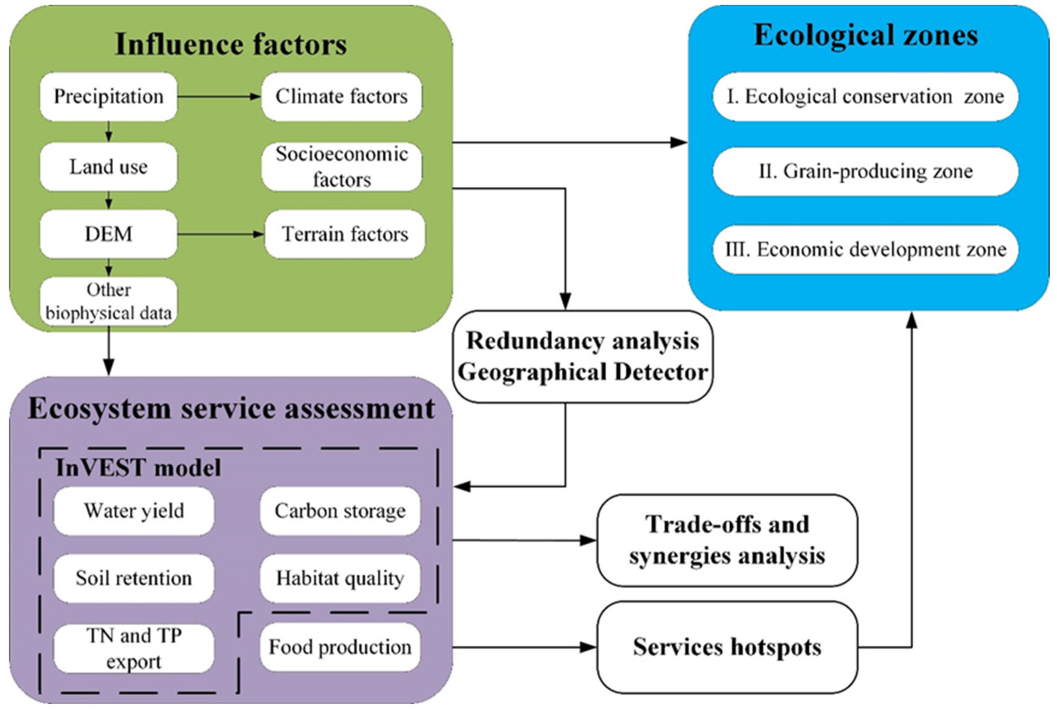
2.2. Research Framework

2.2.1. ES Selection

The analysis of stakeholders to choose relevant ESs, the policy relevance of ESs, and the availability of data serve as the key foundations for the selection of ESs [38,39]. Consideration must be given to the current ecological environment’s characteristics and human welfare in ARB. Combining the ecological characteristics of the basin, such as serious non-point source pollution and soil erosion, abundant water resources, and rich forest resources, our research concentrated on supporting, supplying, and regulating services of ecosystem according to the millennium ecosystem assessment (MEA). Water yield, food production, water purification, soil retention, habitat quality, and carbon storage are selected as ESs to participate in the analysis and discussion.

2.2.2. Influencing Factors

The main core driving factors are human activities and natural factors, both of which constitute pressure on ecosystems [26]. It is necessary to select appropriate factors based on the regional characteristics. Based on the extant scholarly research findings [15,24,26,29,40], and considering the geographical location of ARB, three principles were formulated: (1) regional characteristics, (2) data availability, (3) universality. Therefore, this study chose a total of 14 factors, including climate factors (precipitation, relative humidity, sunshine duration, wind speed, average temperature, and maximum and minimum temperatures), topography factors (elevation and slope), socio-economic factors (rural population and GDP), and human activity factors (land use types and fractional vegetation cover).

2.2.3. Scale Analysis

Assessments of ESs must account for the study scale, which can directly influence the interrelationships between ESs. In general, the research scales contain an administrative scale, a sub-watershed scale, and a pixel scale [41,42]. ESs at different scales have an impact on ecological zoning. We analyzed the ESs at the administrative scale and pixel scale. The administrative scale is town level, which is a more detailed scale. The pixel scale is based on analysis requirements to set up sampling units. The technical roadmap is depicted in Figure 2.

2.3. Methods

2.3.1. InVEST Model

This study used the integrated valuation of ecosystem services and trade-offs (InVEST) model to quantitatively calculate the ESs. This is an open source model, which can be applied in different modules according to the characteristics of the research area. Water yield module, sediment delivery ratio module, nutrient delivery ratio module, carbon storage module, and habitat quality module in the InVEST model calculate the Ess, including water yield (WY), soil retention (SR), water purification (TN and TP export), carbon storage (CS), and habitat quality (HQ). Food production (FP) is a reference to Chen et al. [43]. The module principle and parameters are shown in the Supplementary Information.

2.3.2. Geographical Detector (GD)

A nonlinear statistical technique called GD can be used to identify the variables that influence spatial hierarchical heterogeneity [44]. The degree of heterogeneity was measured by the q statistic. This research focused on the application of the GD’s factor identification module, which detects the spatial heterogeneity of the dependent variable (Y), and the explanatory power of the independent variable (X) to the dependent variable. The formula is as follows:
q = 1 h = 1 L N h σ h 2 N σ 2 = 1 S S W S S T
where h = 1 …L is the number of layers of X, Nh and N are the number of units in corresponding layer h and all units, σ h 2 and σ 2 are the variance of h and Y values of all elements in the corresponding layer, SSW and SST are intralayer variance and total variance of all cells, respectively. The closer the q statistic is to 1, the more explanatory power of X to the heterogeneity of Y [33].

2.4. Statistical Analysis

2.4.1. Redundancy Analysis

We employed redundancy analysis (RDA), which is a constrained ordination technique with Canoco 5.0, to quantify how influencing factors affected ESs and disclosed their relative contributions to ES determination. The advantage of RDA is that it can maintain the contribution of each variable independently [35]. To determine whether linear or unimodal numerical methods should be used, detrended correspondence analysis (DCA) was performed [19]. The gradient’s greatest length along the four axes was 1.1. When the value was less than 3, it made sense to employ a linear model. Consequently, RDA was used. The Monte Carlo methods were used to test the influencing factors.

2.4.2. Pearson Correlation Analysis (PCA)

PCA was employed to investigate the associations among ESs, serving as the foundation for judging trade-offs and synergies [45]. ES trade-off relations occur when the enhancement of one service comes at the expense of diminishing the provision of another service, while ES synergy relations occur when multiple services are simultaneously increased [46]. If the coefficients of the two ESs are negative and pass the significance test (p < 0.05) by correlation analysis, a trade-off relationship is assumed; otherwise, a synergistic relationship is assumed [42,47]. This result was obtained by Origin 2021 and SPSS 25.0.

2.4.3. Services Hotspots

ES hotspots are a specific spatial analysis technique to identify areas of high value. The technique has been extensively utilized for identifying priority regions in ES protection [48]. This study delineated hotspots as each service’s richest 10% of grid cells at the pixel scale. The pixels that were hotspots of each ES were coded to 1, and the remaining pixels were assigned a value of 0. A map with integer pixel values that displayed the quantity of hotspot overlaps between several ESs was created by adding the seven hotspot layers together for each pixel.

2.5. Data Sources

The basis for using 1995 and 2015 as typical years was to highlight the differences in the inter-annual changes of ESs. Meanwhile, the construction of the Xiquanyan reservoir around 1995 changed the pattern of the basin’s ESs, and the ecological regionalization scheme of China was promulgated in an updated version (in 2015). The time span between 1995 and 2015 can fully show the changes of the ESs in the basin, which is in line with China’s objective to formulate steps every five years. So, 1995 and 2015 were selected as the study years. The data were divided into two categories: input data for running the model and supporting influencing factors. The InVEST model’s necessary parameters were obtained from the references or calculations. In Table 1, the data sources are displayed. The spatial data were processed by ArcGIS 9.3.

3. Results

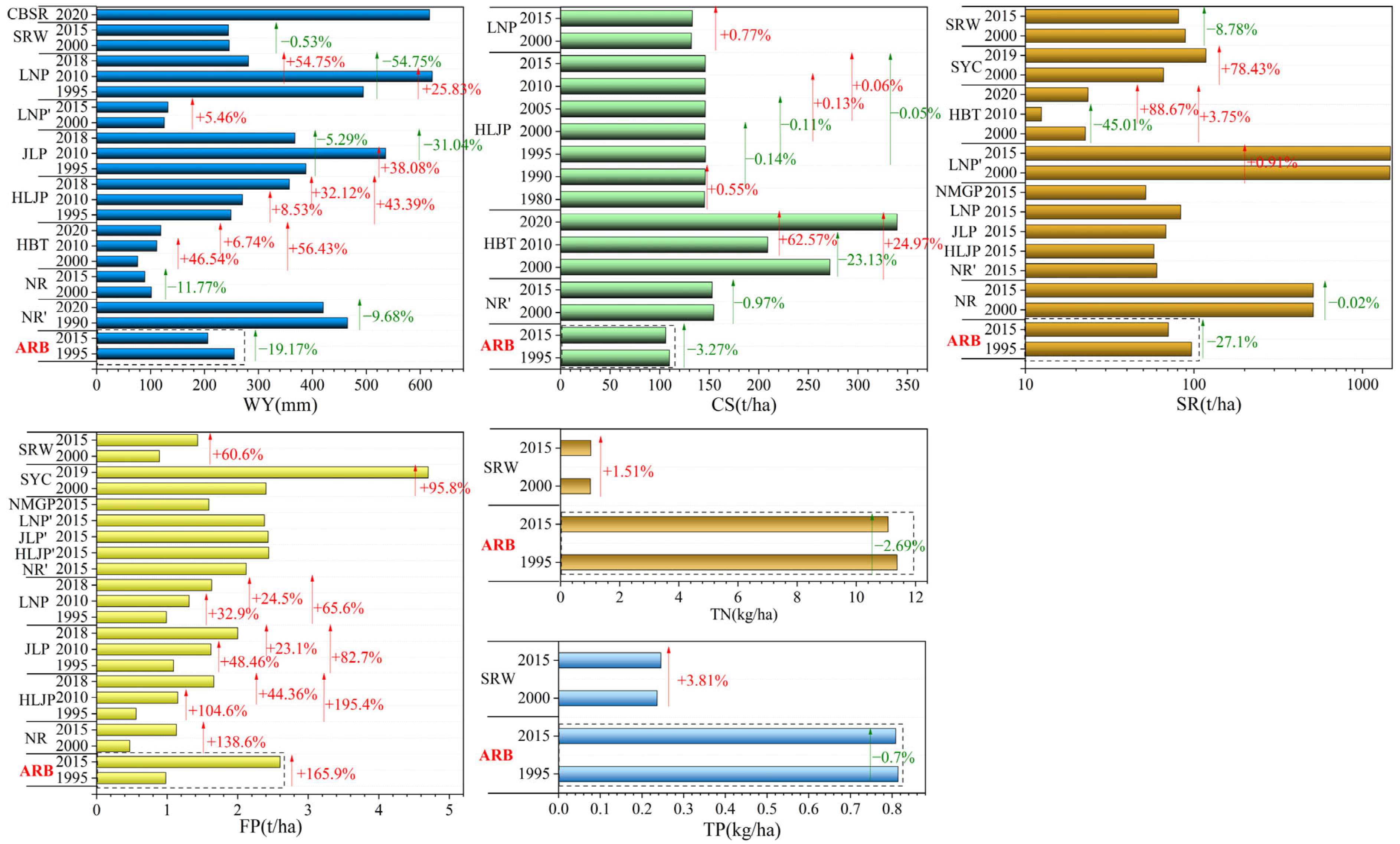
3.1. Spatio-Temporal Changes of ESs

The spatial distribution of ESs and changes between 1995 and 2015 are shown in Figure 3. The total WY in 1995 and 2015 was 9.03 million m3 and 7.32 million m3, which decreased by 18.93%. SR decreased from 34.21 million tons to 24.94 million tons and from 96.58 t/ha to 70.41 t/ha between 1995 and 2015. TN and TP showed a downward trend from 1995 to 2015. They decreased by 108.64 t and 4.87 t, respectively, and the decline rates were 2.70% and 1.69%. TN and TP were 11.37 kg/ha and 0.81 kg/ha in 1995, and 11.07 kg/ha and 0.80 kg/ha in 2015, respectively, with a small change rate. The decreased area accounted for 50.99% and 52.48%. The total CS amount decreased from 38.87 million tons to 37.60 million tons between 1995 and 2015, and CS decreased from 109.74 t/ha to 106.16 t/ha; the change rate was 3.3%. FP of the basin increased by 1.67 times between 1995 and 2015 from 0.98 t/ha to 2.59 t/ha. The area that changed was concentrated in farmland, accounting for 44.97% of the basin. HQ were 0.464 and 0.459 in 1995 and 2015. The changes in areas with increased HQ accounted for 20.05% and decreased HQ accounted for 29.44%.

3.2. Influencing Factors on ESs

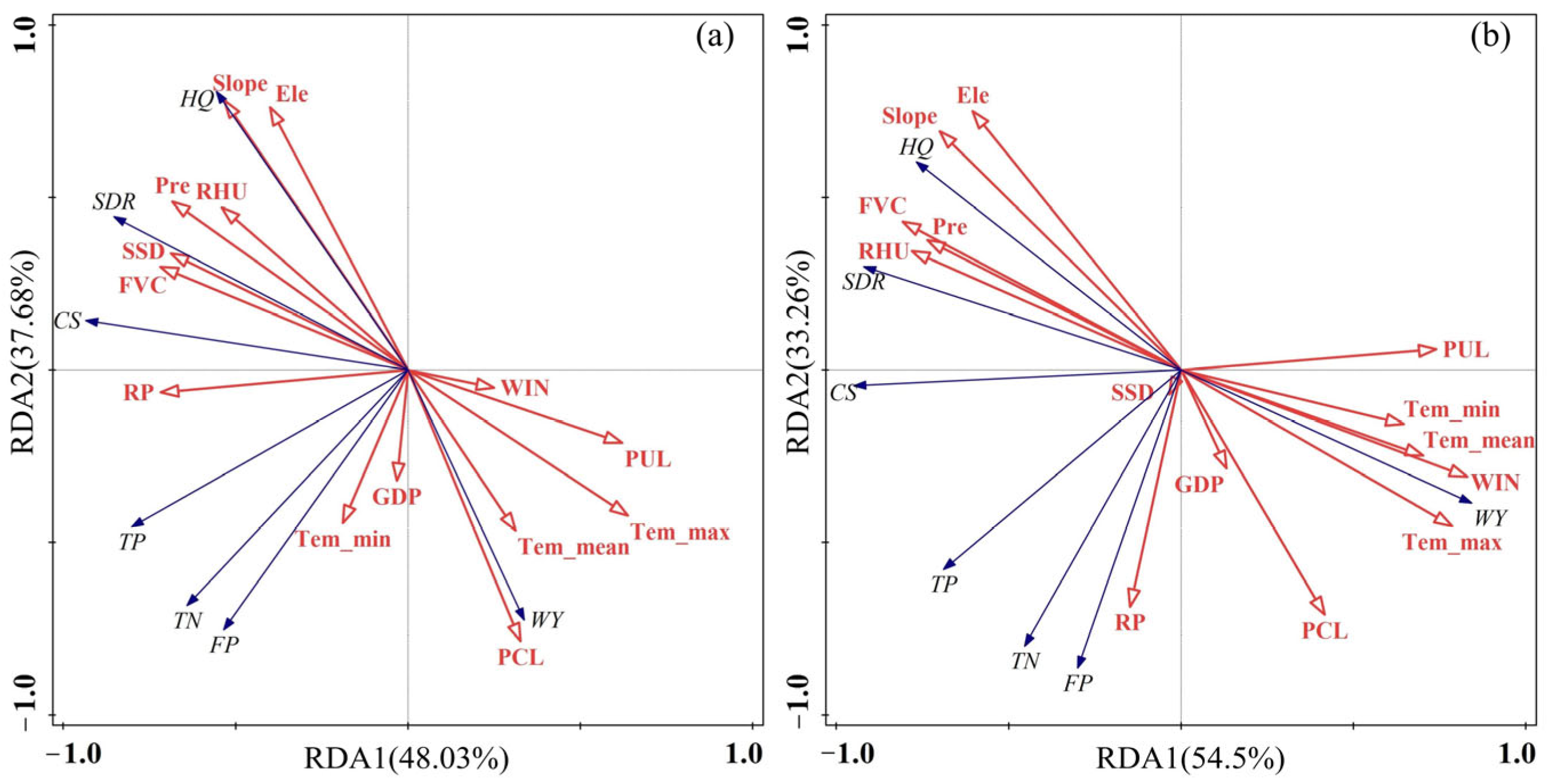
3.2.1. Relationships between Influencing Factors and All ESs

We chose 14 representative factors, and the ESs that are referred to in the above sections were selected for RDA (Figure 4). The explanatory variables accounted for ESs for 94.0% and 91.6% in 1995 and 2015. Among the influencing factors, the contribution of terrain factors (slope) was strongest (39.4% and 46.6% in 1995 and 2015). The positive correlation between slope and HQ was the strongest. In 1995, except for slope, the contribution of the rural population, precipitation, elevation, and land use were 20.3%, 11.9%, 8%, and 11.5%, respectively. Other influencing factors were not significant and were weakly correlated with ESs. The contribution of rural population and land use in 2015 was 14.8% and 21%. From 1995 to 2015, the connections between ESs and affecting factors were unchanged. Based on the RDA biplot, the correlation between meteorological factors and SR was stronger, the correlation between socio-economic factors and TN export, TP export, and FP was stronger, and the correlation between meteorological factors and WY was stronger. The correlation between terrain factors and HQ was stronger.

3.2.2. Individual ES Drivers in Spatial Heterogeneity

The explanatory powers of distinct components in ESs are presented in Figure 5. Except for SSD in 2015, every variable met the significance test requirements (p < 0.05) according to these differentiation and factor detection results, and there was clear regional variability in the ESs. Differences in the ability of driving factors to explain the individual ESs were observed throughout different years. In 1995 and 2015, land use had the most significant influence on the spatial differentiation of WY, TN, TP, CS, FP, and HQ, which was more than 0.7. Meanwhile, the slope variable exhibited the highest level of explanatory power accounting for spatial differentiation, which was 0.48 in 1995 and 2015. The q statistics were ordered for all factors (land use type > terrain factors > vegetation coverage > climatic factors > socio-economic factors).

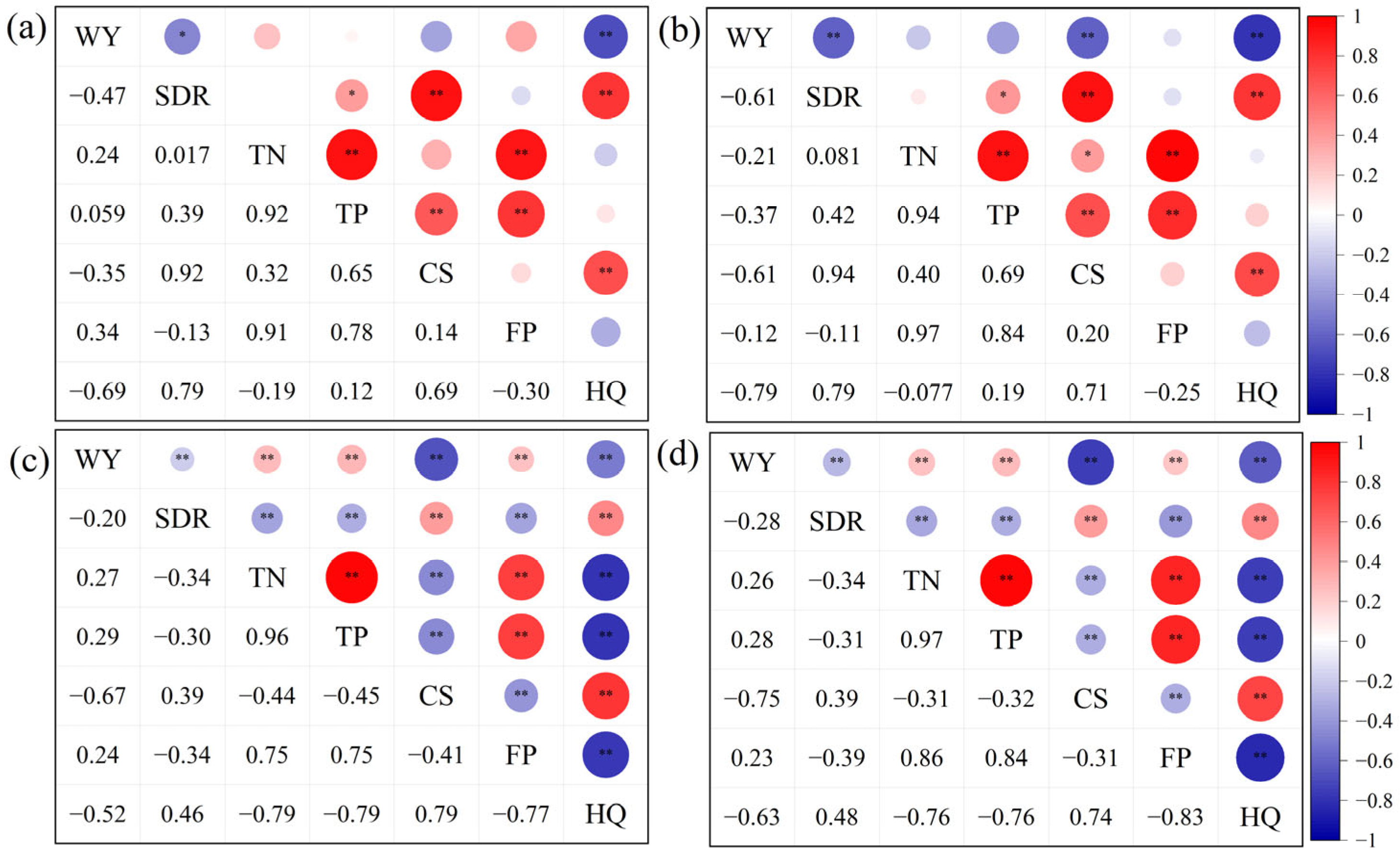
3.3. Interactions among ESs at Various Spatial Scales

The results are visually presented in Figure 6. The findings indicated that most of the correlations at the administrative unit scale were not significant, and the correlations at the pixel scale were all significant. At the administrative unit scale, the synergistic relationship of ESs dominated in 1995 and 2015, and the intensity of correlation between ESs in 2015 was stronger than that in 1995. Merely five pairs of ESs exhibited negative correlation in 1995, with SR and WY, HQ and WY establishing a trade-off connection. Moreover, eight pairs of ESs had a synergistic relationship. Greater than 0.7 correlation values were found between CS and SR, HQ and SR, TN and TP, FP and TN, TP and FP, CS and HQ. The relationship between WY and TN, TP and FP underwent a transition from positive in 1995 to negative in 2015. CS and WY changed into a trade-off relationship, TN and CS changed into a synergistic relationship, and the relationship between other ESs remained unchanged. At the pixel scale, from 1995 to 2015, the correlations between ESs were significant, and the positive and negative correlations did not change. There was a trade-off relationship between 12 pairs of ESs and a synergistic link between 9 pairs of ESs.

3.4. Identification of ES Hotspots at Each Spatial Scale

The integrated hotspots of ESs are displayed at spatial scales in Figure 7. The hotspot overlaps’ spatial distribution in 1995 and 2015 was the same at the pixel scale. Three ES hotspot overlaps occupied the majority, accounting for 51.81% and 50.39% of the entire basin in 1995 and 2015, and were concentrated in the upstream, which was mainly forest. The main ESs were CS, SR, and HQ. The areas of six ES hotspot overlaps accounted for the smallest proportion, which was 6.49% and 4.66% in 1995 and 2015, respectively. The proportion of the area containing two, four, and five ESs hotspot overlaps did not exceed 15%. From 1995 to 2015, the area of one ES hotspot overlap increased significantly, while the area of two ES hotspot overlaps decreased in the spatial distribution.
To strengthen ESs’ management, the mean number of multiple hotspot overlaps in each town-level administrative unit was calculated; the result is shown in Figure 7c,d. From 1995 to 2015, only six administrative units had an increase in the mean number of multiple hotspot overlaps, whereas the majority of administrative units showed a downward trend. The mean number of multiple hotspot overlaps in all administrative units was separated into five levels by applying the natural breakpoint approach. The region with the highest value changed from 6 units to 9 units and the second highest value changed from 8 units to 10 units. The lowest and second lowest values of the regions were mostly located near the downstream outlet of the ARB.

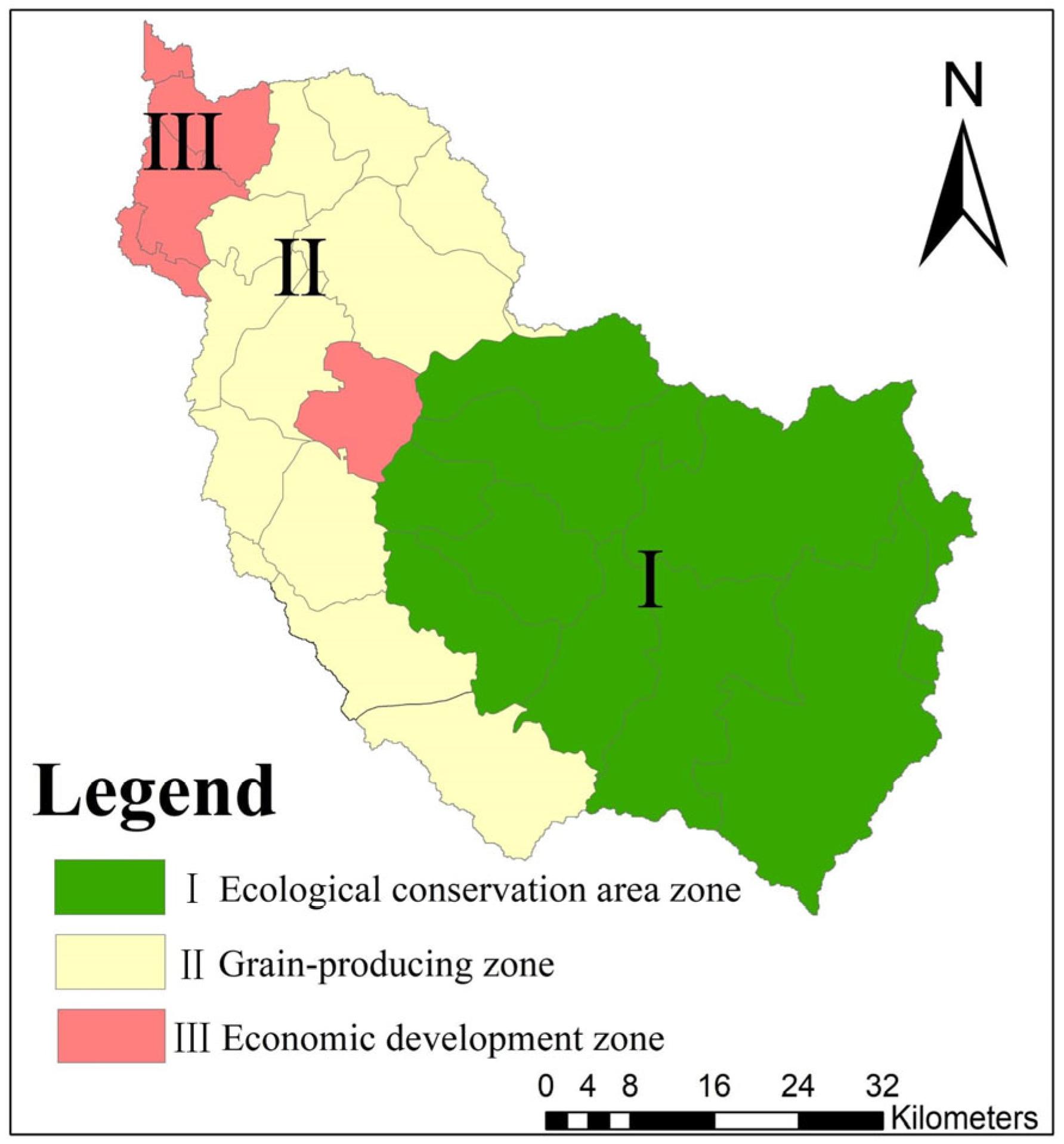
3.5. Results of Ecological Zoning in ARB

ARB’s ecological zones are classified into two levels. The first level is the administrative scale of cluster administrative units by statistical analysis (in Supplementary Information). The second level is the number of multiple hotspot overlaps at each scale. Finally, ARB is divided into three important zones (Figure 8). These zones are as follows: I. Ecological conservation zone. The zone has abundant natural resources and water resources, which provide a large amount of ESs, including the areas with a large number of hotspots. II. Grain-producing zone. The land use category is farmland, with ESs primarily provided by FP. This zone has three to four ES hotspots. III. Economic development zone. This zone has a close relationship with human activities, which is the main region of the urban circle. Moreover, this zone has the fewest multiple ES hotspots, and urban function is the dominant ecological function.

4. Discussion

4.1. Changes in ESs by Land Use Pattern

An essential first step in ecosystem management is the evaluation and analysis of ESs’ geographical distribution characteristics [15]. ESs comprise diverse advantages that are derived by humans from ecosystems, so ES selection is related to stakeholders, policy relevance, and the region’s environmental characteristics [12]. ARB situated in Northeast China is recognized as one of the renowned regions globally known for its mollisols. Therefore, the types of ESs in this region or nearby regions are concentrated. The general selection of ESs is from supporting, cultural, regulating, and provisioning services to conduct research [49]. One supporting service (HQ), two provisioning services (WY and FP), and three regulating services (CS, TN, TP, and SR) were used as main ESs in ARB. ESs have differences in land use in different regions, but making comparisons between research studies is challenging because of variations in scale and methodologies, preventing generalizations of local or regional results [31]. To explore the reasons for such differences, and to facilitate comparison, we sorted out the changes in regulation services, support services, and supply services in Northeast China, which were consistent with the types of ESs in this study. They are shown in Figure 9. Inter-annual changes of ESs across various regions in Northeast China exist differentially, which is significantly associated with land use patterns [50]. The research additionally validated that land use patterns are the essential factor influencing the spatial heterogeneity of ESs. Except for FP, the ESs of ARB showed a downward trend from 1995 to 2015, which was consistent with the overall ES change trend in Northeast China spanning the years 1990 to 2020. However, the pattern of ES changes in surrounding regions (Liaoning Province, Bin County, Jilin Province) and Heilongjiang Province (including the basin) showed inconsistencies with ARB. The reason was mainly related to the cumulative changes of ESs in partial regions at various scales, that is, the cumulative changes of partial regions increased the overall changes at large scales. ARB belongs to the small scale watershed, therefore, land use pattern changes that were subtle led to inter-annual variability in the Ess, producing noticeable changes. The most powerful explanatory factor for spatial differentiation was land use type. Ecosystems’ arrangements and structures are directly impacted by the utilization of land use, ultimately influencing the ability to provide ESs [28]. Environmental protection policy implementation and land use in different regions have resulted in alterations to ESs. Quantifying and comparing ESs under six land use patterns (Table 2) indicated that the primary ecosystems that contributed to the provision of ESs were the farmland ecosystem located downstream and the forest ecosystem situated upstream. In provisioning services, FP was mainly provided by the farmland ecosystem, and WY was provided by farmland and forest ecosystems. In regulating services, the forest ecosystem exhibited the highest soil retention capacity, while the farmland ecosystem demonstrated the least ability to purify water bodies. Additionally, the forest ecosystem boasted the greatest carbon storage capacity. In Northeast China, the continuous development and utilization of black soil resources increased FP in provisioning services in all the research areas [42]. Furthermore, ESs were more directly and significantly impacted by the quick rise of urbanization in land use patterns [51], which reflected that the increased area of WY was concentrated near the outlet of the basin belonging to the urban suburbs of Harbin and was affected by urbanization resulting in changes. Urbanization played a significant role in influencing alterations in land use changes. To sum up, the alterations in ESs were influenced by local and national land use strategies [50].

4.2. Relationships between ESs

Among these ESs, differences in the correlations between ESs at various scales were observed, subsequently influencing the synergistic and trade-off relationships. The correlation between most ESs at the administrative unit scale was weak, with some not even reaching a significant relationship when compared with the pixel scale. The reason was that the pixel scale was aggregated to the administrative unit scale, and the arrangement and composition of land use types were different, determining towns’ ESs [31,59]. Meanwhile, the administrative unit scale obscured some ESs’ spatial heterogeneity that was observed at the pixel scale [60]. Hence, at both the administrative scale and the pixel scale, alterations in significance or direction of correlations between pairs of ESs were detected in the years 1995 and 2015. There were 15 pairs of the same correlation direction of ESs and 6 pairs changed direction in 1995. In 2015, there were 12 pairs with the same correlation direction of ESs and 9 pairs changed direction at different scales. At the same scale, the correlation direction of ESs did not change at the pixel scale, but there were three pairs of ESs at the administrative scale that changed from 1995 to 2015. Changes focused on the inter-relationships between water-related ESs (WY, SR, and NDR), which were influenced by the spatial patterns and quantity of precipitation across various spatial scales. This finding was in line with the findings of Hou, Lü, Chen, and Fu [59]. However, synergistic interactions existed between FP and NDR (TN and TP export), and FP had a trade-off connection with SR and HQ, indicating that when FP increased, water purification ability weakened; moreover, the soil retention ability and habitat quality also declined. The increase in FP at a time when the area of farmland was decreasing was associated with the amount of chemical fertilizer applied, which led to a decrease in soil fertility, an increase in soil erosion, and, consequently a decrease in the amount of SR, leading to a decrease in HQ. Increased FP and agricultural fertilization also increased regional non-point source pollution, raising the potential risk of water pollution [42]. WY had trade-offs with CS, SR, and HQ, respectively. Therefore, it can be seen that there were trade-offs between regulating and supporting services and provisioning services, respectively, and other studies have also proved this result [15,61]. When ESs offer provisioning services to human beings, they do so at the cost of other ESs.
The pixel scale can better judge the relationship between ESs from the perspective of watershed space and natural boundary, while land use policy and ecological management are formulated according to the administrative unit, which can better evaluate the relationship between ESs from a management perspective [62]. Hence, the investigation of these two scales is crucial as it directly pertains to the supply and demand of ESs and the policy-making plans. Similar research has focused more on ESs at a single scale, like the administrative scale [28], the watershed scale [23], and the special geomorphic area [63], further emphasizing the alterations in regional integrity. Studies in multiple scales have involved the grid, watershed, township, sub-catchment, and county scales [31,34]. A finer spatial distribution of ESs resulted from a smaller assessment unit; this caused variations in ESs at various scales, which in turn influenced the synergies and trade-offs between ESs. However, the results in the finer scale reflected the spatial heterogeneity of a single ES in this study, which reflected the practical significance of multi-level analysis methods on the scale of refinement. Therefore, from the perspective of management evaluation, trade-offs and synergies, this study selected both pixel and administrative scales that were convenient for policy formulation and sustainable development of local ESs. The temporal and spatial distribution of ESs was analyzed fundamentally at the pixel scale, and the functional zone policies that met the actual production and living needs were formulated at the administrative scale, providing a scientific basis for the overall control research at a large regional scale.

4.3. Influencing Factors Analysis

The quantitative analysis between ESs and impact factors was not clear enough in the previous research. Understanding the spatial patterns and relationships of influencing factors of ESs is necessary for effective strategies [31]. Spatial distribution variations in ESs are formed under the combined action of influencing factors. Apart from land use as the driving force, the results demonstrated that factors such as human activities, geography, and climate influenced both the overall and individual ESs. The contributions to ESs were higher with slope, precipitation, and population.
Topographic elements exerted a substantial influence on the local climate, land utilization patterns, and vegetation distribution. The more layers of slope and altitude, the more obvious the difference, thereby constituting a significant factor that influenced ESs [15,38]. ARB is a small watershed, which can easily identify slope grade. Hence, the basin exhibited distinct variations in ESs across different slopes, explained by the predominant pattern of land use. Meanwhile, the forest slope was between 15° and 30°, whereas the slope of the farmland and urban land was between 0° and 3°. Soil erosion intensity of more than 3° reached a strong degree, and water and soil conservation measures should be taken above 15° [64], so the regions having a high capability for soil retention were densely clustered in the forest within the upper parts of the basin. The result of GD showed that the driving factor causing the spatial heterogeneity of soil retention was topographic factors, which is in line with the results of Xiao, Hu, and Xiao [35]. The higher the TN and TP export, the weaker water purification ability [65]; therefore, water purifying capability of the farmland ecosystem exhibited the lowest performance. Terrain and precipitation had an impact on the TN and TP export migration process. From 1995 to 2015, ARB’s TN and TP export heterogeneity was strongly correlated with variations in precipitation. Therefore, climatic factors are also important determinants of ESs. RDA results showed that climate factors and ESs had a strong relationship, with a contribution rate of over 10%. The results of other studies have also verified the strong correlation between climate factors and ESs [24,26].
Human activities are another important factor affecting ESs, mainly involving population, GDP, road density, and each land use proportion area [23,66]. In this study, ESs were more strongly impacted by the population and the percentage of urban land. Human activities directly affected the area of farmland, environmental pollution, urbanization, and ecological and environmental protection measures, etc. Human activities affected the land pattern. The transfer matrix showed that notable alterations occurred on the urban land (Table 3), especially in the suburbs of Harbin in the lower reaches and the urban area of Acheng city. As urbanization increased, urban land gradually expanded outwards, and farmland was mainly converted to urban land (100.52 km2). There was a decrease in farmland, which was transferred to forest (80.18 km2). From 1995 to 2015, farmland, forest, and grassland decreased, respectively, to 88.75 km2, 25.72 km2, and 13.98 km2. Water, urban land, and useless land increased, respectively, to 23.90 km2, 65.82 km2, and 38.74 km2. Humans increased food production by increasing the application of chemical fertilizers, but the ability of water purification in the farm ecosystem also weakened. Therefore, the farmland ecosystem was most affected by human activities.

4.4. Sustainable Development Strategy of ESs in Small Basins

In addition to strengthening the evaluation of the geographical and temporal variations of ESs, ecological environment management and construction should be strengthened in small basins. Ecological functional zoning is an effective measure, which is more conducive to the formulation of management strategies. Therefore, regionalizing ecological functions is a key step. This study established a priority protection frame for ESs through hotspots and clustering results of influencing factors.
The ecological zone division was based on the town-level administrative unit in this research. The town-level scale was smaller, which is more feasible to put China’s environmental policies into practice, and the results of ESs’ amount were accurate to more effectively promote the planning of local ecological functional areas [67]. The division method was “bottom to top” [68]. Units with the same functional attributes and units providing the same number hotspots of ESs can be divided into one zone, which is more convenient for policymakers to manage and formulate policies. This is effective for small-scale ecological regionalization. Combined with the development goals of different units, the management responsibilities, and the executive power of policy implementation, the following measures to manage each zone can be taken. I. Ecological conservation zone. Due to the terrain being complex, the quality of forest is reducing, the ability to save water and soil is also reducing, and the forest’s ecological function is weakened, resulting in forest ecosystem function degradation, and the trade-off between WY and SR and HQ changing. Human activities in the zone should be reduced and it is suitable to develop an artificial ecological compensation mechanism to protect the forest ecosystem. Meanwhile, government agencies had better prioritize the surveillance of water quality in the reservoir. The objective is to safeguard the carrying capacity of forest tourism resources within this region and the development of ecotourism and environmental protection infrastructure construction [69]. II. Grain-producing zone. The environmental problems caused by the increase in grain yield are more sloping farmland, heavy soil erosion, and serious damage to the surface morphology and landscape. It is fit for carrying out grain production activities guided by smart, modern, and ecological agriculture, reducing surface pollution from agriculture and enhancing the quality of cultivated soils. III. Economic development zone. The environmental problems are low vegetation coverage and lack of green belts in the suburban junction. This zone needs to be protected and utilized and the construction of ecological environment protection has to be reinforced. Ecosystem zoning can identify areas that require greater ecological protection and management, such as grain-producing zones and economic development zones, and the strictest control measures should be adopted for ecological conservation area zones to ensure the sustainability of ES output [70]. Consequently, in addition to meeting the actual demands, the comprehensive zoning technique based on ES distribution and impacting variables, and the distribution of multiple hotspots in this study, may also be paired with relevant conservation planning.
With the support of current policies, the existing ecological function zoning mainly focuses on ecological function schemes and ecological protection red lines, which is characterized by a macro-scale, and the partitioning method is “top to down” [68]. However, the small basin scale is the underlying key unit of macro-policy implementation, and the approach adopts “down to top” at the fundamental scale. It is worth noting that the macro-policy formulation is based on the condition of the small basin’s ecological environment. This study area is located in Heilongjiang Province. Based on China’s ecological function division that was issued in 2015 [71], the basin is divided into four units in the Level III framework, focusing on ecological functions, including conservation of soil and water. According to the policy of environmental control units in Heilongjiang Province, it is divided into priority protection units, key control units, and general control units. The basin is almost in the priority protection units. This policy emphasizes pollution prevention and control, ecological environment protection, and risk control. It can be seen that the former focuses on the ecosystem function, while the latter focuses on environmental protection. Combined with field investigation, this study is more convenient to divide functional areas based on a small basin scale. The division result is carried out from the perspective of significant ecosystem services, taking into account ecological functions, environmental protection, local economy, etc. The division can not only meet practical needs but can also connect with existing policy, which is scientific and reasonable. This approach can provide a new idea from a new perspective for other similar basin divisions.

5. Conclusions

This research aimed to analyze typical ES spatial distribution characteristics within ARB, and also identify the variables that impact their distribution. The results demonstrated that WY, SR, TN, TP export, CS, and HQ decreased from 1995 to 2015. FP had an increasing trend. The ESs exhibited obvious spatial heterogeneity and land use pattern as the driving factors. Service hotspots showed that the hotspot overlaps’ spatial distribution was identical at the pixel scale. The average number of multiple hotspot overlaps in most administrative units showed a downward trend from 1995 to 2015. The three zones were the economic development zone, grain-producing zone, and ecological conservation zone. This division result provides policymakers with ecological zoning schemes that are conducive to sustainable economic growth and the use of ESs.

Supplementary Materials

The following supporting information can be downloaded at: https://www.mdpi.com/article/10.3390/land13071030/s1, Table S1: Critical parameter settings in the biophysical attributes table; Figure S1. Cluster analysis results.

Author Contributions

Methodology, data collection, data analysis, writing—original draft preparation, X.G.; supervision, modification, L.W.; supervision, Q.F. and F.M. All authors have read and agreed to the published version of the manuscript.

Funding

The research was supported by the Natural Science Foundation of China (52309042), the Natural Science Foundation of Heilongjiang Province (LH2023E004), and the “Young Talents” Project of Northeast Agricultural University (22QC07).

Data Availability Statement

All data generated or analyzed during this study are included in this published article.

Conflicts of Interest

The authors declare no conflicts of interest.

References

  1. Millennium Ecosystem Assessment. Ecosystems and Human Well-Being: Synthesis; Island Press: Washington, DC, USA, 2005. [Google Scholar]
  2. Groot, R.S.d.; Wilson, M.A.; Boumans, R.M.J. A typology for the classification, description and valuation of ecosystem functions, goods and services. Ecol. Econ. 2002, 41, 393–408. [Google Scholar]
  3. Redhead, J.W.; Stratford, C.; Sharps, K.; Jones, L.; Ziv, G.; Clarke, D.; Oliver, T.H.; Bullock, J.M. Empirical validation of the InVEST water yield ecosystem service model at a national scale. Sci. Total Environ. 2016, 569–570, 1418–1426. [Google Scholar] [PubMed]
  4. Malinga, R.; Gordon, L.J.; Jewitt, G.; Lindborg, R. Mapping ecosystem services across scales and continents—A review. Ecosyst. Serv. 2015, 13, 57–63. [Google Scholar]
  5. Li, R.; Shi, Y.; Feng, C.C.; Guo, L. The spatial relationship between ecosystem service scarcity value and urbanization from the perspective of heterogeneity in typical arid and semiarid regions of China. Ecol. Indic. 2021, 132, 108299. [Google Scholar]
  6. Hou, Y.; Li, B.; Muller, F.; Fu, Q.; Chen, W. A conservation decision-making framework based on ecosystem service hotspot and interaction analyses on multiple scales. Sci. Total Environ. 2018, 643, 277–291. [Google Scholar]
  7. Blumstein, M.; Thompson, J.R.; Nally, R.M. Land-use impacts on the quantity and configuration of ecosystem service provisioning in Massachusetts, USA. J. Appl. Ecol. 2015, 52, 1009–1019. [Google Scholar]
  8. Costanza, R.; de Groot, R.; Braat, L.; Kubiszewski, I.; Fioramonti, L.; Sutton, P.; Farber, S.; Grasso, M. Twenty years of ecosystem services: How far have we come and how far do we still need to go? Ecosyst. Serv. 2017, 28, 1–16. [Google Scholar]
  9. Leh, M.D.K.; Matlock, M.D.; Cummings, E.C.; Nalley, L.L. Quantifying and mapping multiple ecosystem services change in West Africa. Agric. Ecosyst. Environ. 2013, 165, 6–18. [Google Scholar]
  10. Li, G.; Fang, C.; Wang, S. Exploring spatiotemporal changes in ecosystem-service values and hotspots in China. Sci. Total Environ. 2016, 545–546, 609–620. [Google Scholar] [CrossRef]
  11. Bukvareva, E.; Zamolodchikov, D.; Kraev, G.; Grunewald, K.; Narykov, A. Supplied, demanded and consumed ecosystem services: Prospects for national assessment in Russia. Ecol. Indic. 2017, 78, 351–360. [Google Scholar] [CrossRef]
  12. Bai, Y.; Ouyang, Z.; Zheng, H.; Li, X.; Zhuang, C.; Jiang, B. Modeling soil conservation, water conservation and their tradeoffs: A case study in Beijing. J. Environ. Sci. 2012, 24, 419–426. [Google Scholar] [CrossRef] [PubMed]
  13. Su, S.; Li, D.; Hu, Y.; Xiao, R.; Zhang, Y. Spatially non-stationary response of ecosystem service value changes to urbanization in Shanghai, China. Ecol. Indic. 2014, 45, 332–339. [Google Scholar] [CrossRef]
  14. Lu, X.; Shi, Y.; Chen, C.; Yu, M. Monitoring cropland transition and its impact on ecosystem services value in developed regions of China: A case study of Jiangsu Province. Land Use Policy 2017, 69, 25–40. [Google Scholar] [CrossRef]
  15. Dou, H.; Li, X.; Li, S.; Dang, D.; Li, X.; Lyu, X.; Li, M.; Liu, S. Mapping ecosystem services bundles for analyzing spatial trade-offs in inner Mongolia, China. J. Clean. Prod. 2020, 256, 120444. [Google Scholar] [CrossRef]
  16. Zhao, M.; He, Z.; Du, J.; Chen, L.; Lin, P.; Fang, S. Assessing the effects of ecological engineering on carbon storage by linking the CA-Markov and InVEST models. Ecol. Indic. 2019, 98, 29–38. [Google Scholar] [CrossRef]
  17. Zhang, Z.M.; Gao, J.F.; Fan, X.Y.; Lan, Y.; Zhao, M.S. Response of ecosystem services to socioeconomic development in the Yangtze River Basin, China. Ecol. Indic. 2017, 72, 481–493. [Google Scholar] [CrossRef]
  18. Qi, X.; Wang, K.L.; Zhang, C.H. Effectiveness of ecological restoration projects in a karst region of southwest China assessed using vegetation succession mapping. Ecol. Eng. 2013, 54, 245–253. [Google Scholar] [CrossRef]
  19. Feng, Q.; Zhao, W.; Fu, B.; Ding, J.; Wang, S. Ecosystem service trade-offs and their influencing factors: A case study in the Loess Plateau of China. Sci. Total Environ. 2017, 607–608, 1250–1263. [Google Scholar] [CrossRef] [PubMed]
  20. Mao, D.; He, X.; Wang, Z.; Tian, Y.; Xiang, H.; Yu, H.; Man, W.; Jia, M.; Ren, C.; Zheng, H. Diverse policies leading to contrasting impacts on land cover and ecosystem services in Northeast China. J. Clean. Prod. 2019, 240, 117961. [Google Scholar] [CrossRef]
  21. Pan, Y.; Xu, Z.R.; Wu, J.X. Spatial differences of the supply of multiple ecosystem services and the environmental and land use factors affecting them. Ecosyst. Serv. 2013, 5, E4–E10. [Google Scholar] [CrossRef]
  22. Jing, H.A.; Liu, Y.H.; He, P.; Zhang, J.Q.; Dong, J.Y.; Wang, Y. Spatial heterogeneity of ecosystem services and it’s influencing factors in typical areas of the Qinghai-Tibet Plateau: A case of Nagqu City. Acta Ecol. Sin. 2021, 42, 2657–2673. (In Chinese) [Google Scholar]
  23. Li, J. Identification of ecosystem services supply and demand and driving factors in Taihu Lake Basin. Environ. Sci. Pollut. Res. 2022, 29, 29735–29745. [Google Scholar] [CrossRef] [PubMed]
  24. Li, J.; Zhou, Z.X. Natural and human impacts on ecosystem services in Guanzhong—Tianshui economic region of China. Environ. Sci. Pollut. Res. 2016, 23, 6803–6815. [Google Scholar] [CrossRef] [PubMed]
  25. Cumming, G.S.; Buerkert, A.; Hoffmann, E.M.; Schlecht, E.; von Cramon-Taubadel, S.; Tscharntke, T. Implications of agricultural transitions and urbanization for ecosystem services. Nature 2014, 515, 50–57. [Google Scholar] [CrossRef] [PubMed]
  26. Li, Z.; Xia, J.; Deng, X.Z.; Yan, H.M. Multilevel modelling of impacts of human and natural factors on ecosystem services change in an oasis, Northwest China. Resour. Conserv. Recycl. 2021, 169, 105474. [Google Scholar] [CrossRef]
  27. Su, C.; Fu, B. Evolution of ecosystem services in the Chinese Loess Plateau under climatic and land use changes. Glob. Planet. Change 2013, 101, 119–128. [Google Scholar] [CrossRef]
  28. Bai, Y.; Ochuodho, T.O.; Yang, J. Impact of land use and climate change on water-related ecosystem services in Kentucky, USA. Ecol. Indic. 2019, 102, 51–64. [Google Scholar] [CrossRef]
  29. Liu, Z.T.; Wu, R.; Chen, Y.X.; Fang, C.L.; Wang, S.J. Factors of ecosystem service values in a fast-developing region in China: Insights from the joint impacts of human activities and natural conditions. J. Clean. Prod. 2021, 297, 126588. [Google Scholar] [CrossRef]
  30. Luo, Q.; Zhou, J.; Li, Z.; Yu, B. Spatial differences of ecosystem services and their driving factors: A comparation analysis among three urban agglomerations in China’s Yangtze River Economic Belt. Sci. Total Environ. 2020, 725, 138452. [Google Scholar] [CrossRef]
  31. Sun, X.; Shan, R.; Liu, F. Spatio-temporal quantification of patterns, trade-offs and synergies among multiple hydrological ecosystem services in different topographic basins. J. Clean. Prod. 2020, 268, 122338. [Google Scholar] [CrossRef]
  32. Zhang, Z.Y.; Liu, Y.F.; Wang, Y.H.; Liu, Y.L.; Zhang, Y.; Zhang, Y. What factors affect the synergy and tradeoff between ecosystem services, and how, from a geospatial perspective? J. Clean. Prod. 2020, 257, 120454. [Google Scholar] [CrossRef]
  33. Zhang, C.; Li, J.; Zhou, Z.; Sun, Y. Application of ecosystem service flows model in water security assessment: A case study in Weihe River Basin, China. Ecol. Indic. 2021, 120, 106974. [Google Scholar] [CrossRef]
  34. Pan, N.H.; Guan, Q.Y.; Wang, Q.Z.; Sun, Y.F.; Li, H.C.; Ma, Y.R. Spatial Differentiation and Driving Mechanisms in Ecosystem Service Value of Arid Region: A case study in the middle and lower reaches of Shule River Basin, NW China. J. Clean. Prod. 2021, 319, 128718. [Google Scholar] [CrossRef]
  35. Xiao, Q.; Hu, D.; Xiao, Y. Assessing changes in soil conservation ecosystem services and causal factors in the Three Gorges Reservoir region of China. J. Clean. Prod. 2017, 163, S172–S180. [Google Scholar] [CrossRef]
  36. Bennett, E.M.; Peterson, G.D.; Gordon, L.J. Understanding relationships among ecosystem services. Ecol. Lett. 2009, 12, 054020. [Google Scholar] [CrossRef] [PubMed]
  37. Liu, X.; Burrascharles, L.; Kravchenkoyuri, S. Overview of Mollisols in the world: Distribution, land use and management. Can. J. Soil Sci. 2012, 92, 383–402. [Google Scholar] [CrossRef]
  38. Fang, Z.; Bai, Y.; Jiang, B.; Alatalo, J.M.; Liu, G.; Wang, H. Quantifying variations in ecosystem services in altitude-associated vegetation types in a tropical region of China. Sci. Total Environ. 2020, 726, 138565. [Google Scholar] [CrossRef] [PubMed]
  39. Daw, T.; Brown, K.; Rosendo, S.; Pomeroy, R. Applying the ecosystem services concept to poverty alleviation: The need to disaggregate human well-being. Environ. Conserv. 2011, 38, 370–379. [Google Scholar] [CrossRef]
  40. Lyu, R.; Clarke, K.C.; Zhang, J.; Feng, J.; Jia, X.; Li, J. Spatial correlations among ecosystem services and their socio-ecological driving factors: A case study in the city belt along the Yellow River in Ningxia, China. Appl. Geogr. 2019, 108, 64–73. [Google Scholar] [CrossRef]
  41. Pan, J.; Wei, S.; Li, Z. Spatiotemporal pattern of trade-offs and synergistic relationships among multiple ecosystem services in an arid inland river basin in NW China. Ecol. Indic. 2020, 114, 106345. [Google Scholar] [CrossRef]
  42. Yang, S.L.; Bai, Y.; Alatalo, J.M.; Wang, H.M.; Jiang, B.; Liu, G.; Chen, J.Y. Spatio-temporal changes in water-related ecosystem services provision and trade-offs with food production. J. Clean. Prod. 2021, 286, 125316. [Google Scholar] [CrossRef]
  43. Chen, T.; Feng, Z.; Zhao, H.; Wu, K. Identification of ecosystem service bundles and driving factors in Beijing and its surrounding areas. Sci. Total Environ. 2020, 711, 134687. [Google Scholar] [CrossRef] [PubMed]
  44. Deng, C.; Zhu, D.; Nie, X.; Liu, C.; Zhang, G.; Liu, Y.; Li, Z.; Wang, S.; Ma, Y. Precipitation and urban expansion caused jointly the spatiotemporal dislocation between supply and demand of water provision service. J. Environ. Manag. 2021, 299, 113660. [Google Scholar] [CrossRef] [PubMed]
  45. Wang, L.; Zheng, H.; Wen, Z.; Liu, L.; Robinson, B.E.; Li, R.N.; Li, C.; Kong, L.Q. Ecosystem service synergies/trade-offs informing the supply-demand match of ecosystem services: Framework and application. Ecosyst. Serv. 2019, 37, 100939. [Google Scholar] [CrossRef]
  46. Raudsepp-Hearne, C.; Peterson, G.D.; Bennett, E.M. Ecosystem service bundles for analyzing tradeoffs in diverse landscapes. PNAS 2010, 107, 5242–5247. [Google Scholar] [CrossRef] [PubMed]
  47. Cornelius, J.; Juergen, K.; Joachim, M.; Thomas, K. Interactions among ecosystem services across Europe: Bagplots and cumulative correlation coefficients reveal synergies, trade-offs, and regional patterns. Ecol. Indic. 2014, 49, 46–52. [Google Scholar] [CrossRef]
  48. Wang, J.; Zhou, W.; Pickett, S.T.A.; Yu, W.; Li, W. A multiscale analysis of urbanization effects on ecosystem services supply in an urban megaregion. Sci. Total Environ. 2019, 662, 824–833. [Google Scholar] [CrossRef] [PubMed]
  49. Li, T.; Lv, Y.; Fu, B.; Hu, W.; Comber, A.J. Bundling ecosystem services for detecting their interactions driven by large-scale vegetation restoration: Enhanced services while depressed synergies. Ecol. Indic. 2019, 99, 332–342. [Google Scholar] [CrossRef]
  50. Li, H.; Mao, D.; Li, X.; Wang, Z.; Jia, M.; Huang, X.; Xiao, Y.; Xiang, H. Understanding the contrasting effects of policy-driven ecosystem conservation projects in northeastern China. Ecol. Indic. 2022, 135, 108578. [Google Scholar] [CrossRef]
  51. Pan, Z.; Wang, J. Spatially heterogeneity response of ecosystem services supply and demand to urbanization in China. Ecol. Eng. 2021, 169, 106303. [Google Scholar] [CrossRef]
  52. Wang, H.; Wang, W.J.; Liu, Z.; Wang, L.; Zhang, W.; Zou, Y.; Jiang, M. Combined effects of multi-land use decisions and climate change on water-related ecosystem services in Northeast China. J. Environ. Manag. 2022, 315, 115131. [Google Scholar] [CrossRef] [PubMed]
  53. Xiang, H.; Zhang, J.; Mao, D.; Wang, Z.; Qiu, Z.; Yan, H. Identifying spatial similarities and mismatches between supply and demand of ecosystem services for sustainable Northeast China. Ecol. Indic. 2022, 134, 108501. [Google Scholar] [CrossRef]
  54. Zhang, X.; Dong, L.; Huang, Y.; Xu, Y.; Qin, H.; Qiao, Z. Equilibrium Relationship between Ecosystem Service Supply and Consumption Driven by Economic Development and Ecological Restoration. Sustainability 2021, 13, 1486. [Google Scholar] [CrossRef]
  55. Li, X.; Huang, C.; Jin, H.; Han, Y.; Kang, S.; Liu, J.; Cai, H.; Hu, T.; Yang, G.; Yu, H.; et al. Spatio-Temporal Patterns of Carbon Storage Derived Using the InVEST Model in Heilongjiang Province, Northeast China. Front. Earth Sci. 2022, 10, 846456. [Google Scholar] [CrossRef]
  56. Ning, J.; Shi, D.; Zhou, S.; Xia, Z. Spatial and temporal patterns of ecosystem services and trade-off synergistic relationships in Bin County, Heilongjiang Province. Res. Soil Water Conserv. 2022, 29, 293–300. (In Chinese) [Google Scholar] [CrossRef]
  57. Gan, S.; Xiao, Y.; Qin, K.; Liu, J.; Xu, J.; Wang, Y.; Niu, Y.; Huang, M.; Xie, G. Analyzing the Interrelationships among Various Ecosystem Services from the Perspective of Ecosystem Service Bundles in Shenyang, China. Land 2022, 11, 515. [Google Scholar] [CrossRef]
  58. Wang, H.; Wang, W.; Wang, L.; Ma, S.; Liu, Z.; Zhang, W.; Zou, Y.; Jiang, M. Impacts of Future Climate and Land Use/Cover Changes on Water-Related Ecosystem Services in Changbai Mountains, Northeast China. Front. Ecol. Evol. 2022, 10, 854497. [Google Scholar] [CrossRef]
  59. Hou, Y.; Lv, Y.; Chen, W.; Fu, B. Temporal variation and spatial scale dependency of ecosystem service interactions: A case study on the central Loess Plateau of China. Landsc. Ecol. 2017, 32, 1201–1217. [Google Scholar] [CrossRef]
  60. Cui, F.; Tang, H.; Zhang, Q.; Wang, B.; Dai, L. Integrating ecosystem services supply and demand into optimized management at different scales: A case study in Hulunbuir, China. Ecosyst. Serv. 2019, 39, 100984. [Google Scholar] [CrossRef]
  61. Li, J.; Bai, Y.; Alatalo, J.M. Impacts of rural tourism-driven land use change on ecosystems services provision in Erhai Lake Basin, China. Ecosyst. Serv. 2020, 42, 101081. [Google Scholar] [CrossRef]
  62. Cord, A.F.; Bartkowski, B.; Beckmann, M.; Dittrich, A.; Hermans-Neumann, K.; Kaim, A.; Lienhoop, N.; Locher-Krause, K.; Priess, J.; Schröter-Schlaack, C.; et al. Towards systematic analyses of ecosystem service trade-offs and synergies: Main concepts, methods and the road ahead. Ecosyst. Serv. 2017, 28, 264–272. [Google Scholar] [CrossRef]
  63. Feng, Q.; Zhao, W.; Hu, X.; Liu, Y.; Daryanto, S.; Cherubini, F. Trading-off ecosystem services for better ecological restoration: A case study in the Loess Plateau of China. J. Clean. Prod. 2020, 257, 120469. [Google Scholar] [CrossRef]
  64. SL446-2009; Techniques Standard for Comprehensive Control of Soil Erosion in the Black Soil Region. Chinese Ministry of Water Resources: Beijing, China, 2009.
  65. Liang, J.; Li, S.; Li, X.D.; Li, X.; Liu, Q.; Meng, Q.F.; Lin, A.Q.; Li, J.J. Trade-off analyses and optimization of water-related ecosystem services (WRESs) based on land use change in a typical agricultural watershed, southern China. J. Clean. Prod. 2021, 279, 123851. [Google Scholar] [CrossRef]
  66. Hu, X.; Hong, W.; Qiu, R.; Hong, T.; Chen, C.; Wu, C. Geographic variations of ecosystem service intensity in Fuzhou City, China. Sci. Total Environ. 2015, 512–513, 215–226. [Google Scholar] [CrossRef] [PubMed]
  67. Sun, X.; Yang, P.; Tao, Y.; Bian, H. Improving ecosystem services supply provides insights for sustainable landscape planning: A case study in Beijing, China. Sci. Total Environ. 2022, 802, 149849. [Google Scholar] [CrossRef] [PubMed]
  68. Smith, M.L.; Carpenter, C. Application of the USDA Forest Service National Hierarchical Framework of Ecological Units at the sub-regional level: The New England-New York example. Env. Monit Assess 1996, 39, 187–198. [Google Scholar] [CrossRef] [PubMed]
  69. Mo, W.; Zhao, Y.; Yang, N.; Xu, Z. Ecological function zoning based on ecosystem service bundles and trade-offs: A study of Dongjiang Lake Basin, China. Environ. Sci. Pollut. Res. 2023, 30, 40388–40404. [Google Scholar] [CrossRef]
  70. He, J.; Yan, Z.Y.; Wan, Y. Trade-offs in ecosystem services based on a comprehensive regionalization method: A case study from an urbanization area in China. Environ. Earth Sci. 2018, 77, 179. [Google Scholar] [CrossRef]
  71. National Ecological Function Division (Modified Edition); Chinese Academy of Sciences, State Environmental Protection Administration, Beijing. 2015. Available online: https://www.mee.gov.cn/gkml/hbb/bgg/201511/t20151126_317777.htm (accessed on 3 July 2024).
Figure 1. Location of ARB in northeast China and administrative units.
Land 13 01030 g001
Figure 2. Technical roadmap.
Land 13 01030 g002
Figure 3. Spatial distribution and variations of ESs from 1995 to 2015.
Land 13 01030 g003
Figure 4. RDA biplot between all ESs and influencing factors in 1995 (a) and 2015 (b).
Land 13 01030 g004
Figure 5. Effects of influencing factors on the spatial variability of ESs in 1995 (a) and 2015 (b).
Land 13 01030 g005
Figure 6. Pearson correlation analysis between pairs of ESs from 1995 to 2015. Notes: (a,b) are representative of the administrative scale in 1995 and 2015; (c,d) are representative of the pixel scale in 1995 and 2015.
Land 13 01030 g006
Figure 7. Number of multiple ESs hotspot overlaps. Notes: (a,b) represent the pixel scale in 1995 and 2015; (c,d) represent the administrative scale in 1995 and 2015.
Land 13 01030 g007
Figure 8. Spatial distributions of ecosystem functional zones in ARB at the administrative scale.
Land 13 01030 g008
Figure 9. Northeast Region (NR and NR’) [20,52,53], Liaoning Province (LNP and LNP’), Heilongjiang Province (HLJP), Jilin Province (JLP), and Inner Mongolia Province (NMGP) [50,53,54,55], Bin town in Harbin (HBT) [56], Shenyang City (SYC) [57], Songhua River watershed (SRW) [42], Changbai Mountain region (CBSR) [58].
Land 13 01030 g009
Table 1. Sources of requirement data.
DataSourcesRelated Model and Factors
Land use typeResource and Environment Science and Data Center (http://www.resdc.cn) (accessed on 15 May 2023)WY, SR, TN, TP, CS, HQ, FP, proportion of urban and farmland.
Climate factorsChina Meteorological Science Data Center (http://data.cma.cn/) (accessed on 6 June 2023)WY, SR, TN, TP, precipitation, relative humidity, sunshine duration, wind speed, average temperature, maximum and minimum temperatures
Digital elevation model (DEM)Geospatial Data Cloud (http://www.gsclound.cn) (accessed on 7 August 2023)TN, TP, SR, elevation, slope
Normalized difference vegetation index (NDVI)United States Geological Survey (USGS) (https://earthexplorer.usgs.gov/) (accessed on 10 September 2023)FP, FVC
GDP, rural population (RP), and food productionHarbin Yearbooks (http://www.harbin.gov.cn/) (accessed on 15 September 2023)GDP, RP, FP
Administrative unitStandard map service (Ministry of Natural Resources of the People’s Republic of China)--
Other parametersThe literature and the InVEST user’s guide (https://naturalcapitalproject.stanford.edu/software/invest) (12 December 2022)WY, SR, CS, HQ, TN, TP
Table 2. Amount of ESs under different land use types.
YearLand Use TypeWY (108 m3)SR (t/ha)TN (kg/ha)TP (kg/ha)CS (t/ha)FP (t/ha)HQ
1995Farmland4.6117.7723.171.4292.602.050.00
Forest3.36190.490.350.24142.000.000.99
Grassland0.10103.601.600.1991.880.001.00
Water0.006.250.080.000.000.000.99
Urban land0.9210.902.640.484.350.000.00
Useless land0.0513.690.870.004.290.000.00
2015Farmland3.6212.7623.641.4592.605.740.00
Forest2.35142.610.340.24142.000.000.99
Grassland0.0440.751.310.1591.880.000.97
Water0.003.690.040.000.000.000.99
Urban land1.128.312.770.504.350.000.00
Useless land0.1910.811.300.014.290.000.00
Table 3. Conversion matrix of land use from 1995 to 2015 (km2).
19952015
GrasslandFarmlandUrban LandForestWaterUseless LandTotal
Grassland2.278.940.3228.670.200.6241.02
Farmland17.021453.14100.5280.1810.7728.211689.85
Urban land0.0643.28133.942.230.222.01181.74
Forest7.2993.0511.461466.618.6617.021604.09
Water0.410.630.070.2112.33013.64
Useless land02.061.250.475.352.3211.45
Total27.041601.09247.561578.3737.5450.193541.79
Disclaimer/Publisher’s Note: The statements, opinions and data contained in all publications are solely those of the individual author(s) and contributor(s) and not of MDPI and/or the editor(s). MDPI and/or the editor(s) disclaim responsibility for any injury to people or property resulting from any ideas, methods, instructions or products referred to in the content.

