Article

Relationship between Ecosystem-Services Trade-Offs and Supply–Demand Balance along a Precipitation Gradient: A Case Study in the Central Loess Plateau of China

1
College of Resources and Environment, Shanxi University of Finance and Economics, Taiyuan 030006, China
2
Key Laboratory of Land Consolidation and Rehabilitation, Land Consolidation and Rehabilitation Center (Land Science and Technology Innovation Center), Ministry of Natural Resources, Beijing 100035, China
*
Author to whom correspondence should be addressed.
Land 2024, 13(7), 1057; https://doi.org/10.3390/land13071057
Submission received: 9 June 2024 / Revised: 4 July 2024 / Accepted: 11 July 2024 / Published: 15 July 2024

Abstract

:
Although the theory of ecosystem services (ESs) is important for guiding land-use planning, knowledge of ESs trade-offs and supply–demand mechanisms is still lacking, and the characteristics of the correlation between the size of trade-offs and the balance between supply and demand along the precipitation gradient have not yet been clarified. In order to supplement this area of knowledge of ESs, we selected 30 small watersheds in high-, medium- and low-precipitation areas as study units. A biophysical model and socio-economic data were used to calculate supply and demand for carbon sequestration, soil conservation and water yield. Redundancy analysis and regression analysis were used to study the ESs trade-offs, the supply–demand dynamics, and the characteristics of their correlation. The results were as follows. (1) The supply and balance between supply and demand of the three ESs, the trade-off between carbon sequestration and water yield and the trade-off between soil conservation and water yield trended downwards from the high-precipitation area to the medium-precipitation area to the low-precipitation area. (2) The primary factors influencing balance between supply and demand with regard to carbon sequestration in high-, medium- and low-precipitation areas were population density and soil organic-matter content, and the size of the conditional effects were greater than 53%. The dominant factor affecting the balance between supply and demand with regard to soil conservation in the three precipitation areas was slope gradient, and the conditional effect was greater than 40%. The most significant determinants of balance between supply and demand with regard to water yield in the three precipitation areas were grassland area, forest area and precipitation, and the conditional effects were greater than 22%. (3) The most significant determinants of the trade-off between carbon sequestration and water yield in high-, medium- and low-precipitation areas were forest, soil organic-matter content and population density, and the conditional effects were all greater than 45%; the primary factors affecting the trade-off between soil conservation and water yield in high-, medium- and low-precipitation areas were grassland and slope gradient, and the conditional effects were all greater than 24%. (4) The relationship between the balance between supply and demand and trade-off size often followed a quadratic function; the next-most-common relationship was a monotonous nonlinear response, and a linear response relationship was relatively rare. This study revealed the factors influencing balance between supply and demand and trade-offs with regard to ESs and the characteristics of their correlations in areas with different degrees of precipitation, which provided a new idea for the synchronous regulation of ESs in the context of conflicts and supply–demand imbalance.

1. Introduction

Ecosystem services (ESs) refer to the direct and indirect advantages that humans derive from ecosystems [1]. ESs can be categorized into four types: provisioning, regulating, supporting, and cultural services [2]. The trade-offs of ESs had been widely regarded as a concern by natural-resource managers. The concept of a trade-off denotes a situation where the improvement in the availability of one ecosystem service (ES) comes at the expense of the availability of another, resulting in an observable pattern where an increase in one ES is accompanied by a decrease in another [2,3]. The studies mainly focus on the relationship between supply and regulation services, as well as that between agricultural production and biodiversity, and the driving forces and regulation of ESs trade-offs are important issues [4,5,6]. The demand for ESs involves the consumption and usage of the products and services produced by the ecosystem. The concept of supply and demand reflects the process in which ESs flow from the natural ecosystem to human uses [7] and is an important basis for urban and rural planning, land-use optimization and tourism management [8,9,10]. The theories of supply and demand and trade-offs with regard to ESs have become important tools for social ecosystem management, which helps to reasonably allocate natural resources, promote human well-being and support the sustainability of the socio-ecological system [11,12,13]. Therefore, supply and demand and trade-offs with regard to ESs have become the frontier and a hotspot of study in geography and ecology [7,14].
Clarifying the key drivers of trade-offs of ESs is the basis of socio-ecological system management, but the research on driving forces is still relatively insufficient. Meanwhile, how does the size of trade-offs respond to the supply–demand balance? In other words, what is the correlation between the trade-off size and the supply–demand balance? This is a new and easily overlooked scientific problem. Certain academics have delved into approaches for aligning the supply and demand for ecosystem services, and these approaches are grounded in the understanding of their trade-off dynamics. ESs trade-offs have been taken as the foundations, constraint conditions or regulating approaches in studies of the supply–demand relationship [15,16,17,18]; these studies formed part of a useful attempt to analyze the correlation between trade-offs and balance between supply and demand in ESs. However, the mechanism of the correlation between trade-offs and balance between supply and demand has not been quantitatively clarified.
The association between the balance between supply and demand and trade-offs in ESs is intrinsic. In the first place, we can see that the enhancement of one ES comes at the cost of reducing another ES when a trade-off occurs. The reduced service is likely to be unable to meet the demand due to insufficient supply, which results in a supply–demand imbalance. Such an outcome indicates that the characteristics of ESs trade-offs have an impact on the dynamics of supply and demand. In the second place, the relationship between supply and demand will also influence the size of the trade-off. For example, when there is an imbalance between wood supply and demand, local residents tend to increase the amount of wood supply through forest harvesting, but, as a result, the carbon-sequestration capacity of the forest will be reduced (this is a trade-off between wood supply and carbon sequestration) [19,20]. The above analysis shows that the relationship between supply-and-demand and trade-offs in ESs is logically valid. This association can manifest not only as synchronization, lag or an inverse relationship between the two over time, but also as a regular spatial pattern of trade-off and supply–demand in different locations. Therefore, clarifying the driving mechanisms of trade-offs and supply–demand in ESs and characterizing the linkage between the size of trade-offs and the degree of supply–demand congruence are helpful for comprehensively understanding supply conflict and supply–demand matching in ESs. Overall, the idea of a study coupling supply–demand and trade-offs is a new one that will provide potential solutions for simultaneously relieving conflicts and supply–demand imbalances with regard to ESs.
The Converting Farmland to Forest Program (CFFP) was implemented to control soil loss and has been in place since 1999 in the Loess Plateau of China. A typical ESs trade-off problem had been recognized: CFFP promoted the healthy development of the ecosystem as a whole, and vegetation cover, soil conservation and carbon storage capacity had been on the rise, yet there had been a decline in both water yield and soil-moisture levels [21,22]. The phenomenon of large-area decline of artificial forest had been found because of water shortage, and the net primary productivity in this area was close to the critical value of the water-resources carrying capacity [23]. Some scholars have proposed that it is necessary to be cautious in returning farmland to forests [24]. It can be seen that the result of this ESs trade-off is the continuous reduction of water yield, and one possible consequence is that the water supply will not meet the needs of ecological, production and domestic water use. How can managers coordinate the relationship between soil conservation, carbon sequestration and water yield and balance in terms of supply and demand? This is a key scientific issue in the study of ESs in the Loess Plateau, and a study examining the link between balance between supply and demand and trade-offs will be an effective way to solve this problem.
It is worth noting that the distributions of precipitation, soil and vegetation exhibit obvious gradients in the Loess Plateau. Annual rainfall diminishes progressively from 700 mm in the southeast to just 200 mm in the northwestern areas, with precipitation lines running almost parallel across the central Loess Plateau. The soil texture gradually becomes coarse, showing a zonal distribution; additionally, the soil’s water-holding capacity decreases, the evaporation increases, and the degree of soil drying becomes more serious from the southeast to the northwest. Accordingly, as precipitation and soil composition vary across zones, the vegetation transitions sequentially from dense forest through forest steppe to dry steppe, desert steppe and steppe desert [25]. Therefore, the systematic study of balance between supply and demand and trade-offs in ESs needs to incorporate the gradient characteristics of the geographical environment in the Loess Plateau. Previous research encompasses the qualitative assessment of trade-offs and synergies among ESs, an examination of the spatial patterns in trade-off size and the degree of supply–demand alignment, as well as exploration of the mechanisms behind trade-offs and simulations across various scenarios [26,27,28,29]. However, the characteristics of the correlation between supply–demand dynamics and trade-offs across the precipitation gradient were unclear, and there is still a lack of a theoretical basis for ecosystem management across different gradients.
In summary, the characteristics of the correlation between supply–demand dynamics and trade-offs in ESs, especially the spatial differentiation of the characteristics along the precipitation gradient, are still research gaps in the field of ESs that hinder the optimal management of land resources at the landscape scale. Therefore, we selected 30 small watersheds in high-precipitation (mean annual precipitation greater than 500 mm but less than 600 mm), medium-precipitation (mean annual precipitation greater than 400 mm but less than 500 mm), and low-precipitation (mean annual precipitation greater than 300 mm but less than 400 mm) areas in the central Loess Plateau. We used biophysical models and socio-economic data to estimate the supply and demand of water yield, carbon sequestration and soil conservation, and we used redundancy analysis and the surface fitting in data analysis. The aims of this research were to (1) uncover how supply–demand dynamics and trade-offs dynamics vary spatially across regions characterized by different levels of precipitation, (2) reveal the main factors affecting supply–demand balance and the size of trade-offs, (3) elucidate the characteristics of the relationship between the supply–demand balance and the size of trade-offs and explore the underlying mechanism.

2. Materials and Methods
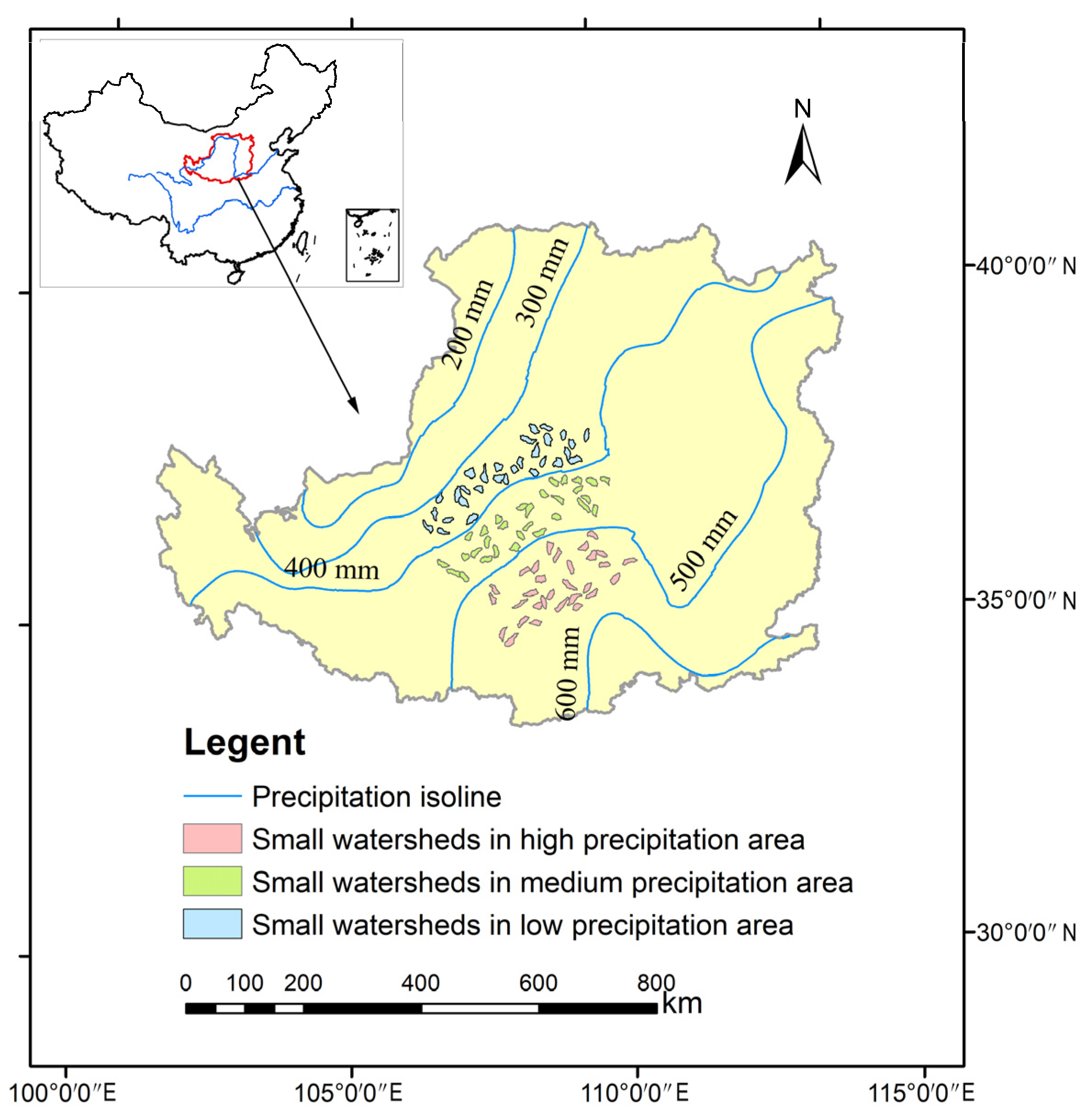
2.1. Study Area

The Loess Plateau is a significant loess deposit in China where loess has been accumulating since the Quaternary. Loess is a weathering product with relatively uniform particle distribution and relatively loose structure. Consequently, the Loess Plateau stands out as one of the regions most severely affected by soil erosion globally. The Loess Plateau is dominated by continental monsoon climate, with an average annual temperature of 4–12 °C. The spatial and temporal distribution of rainfall is extremely uneven; more than 60% of the annual rainfall occurs during July-September. The vegetation type has a zonal distribution, and the natural vegetation has been seriously damaged, but the vegetation coverage has increased significantly since the implementation of the Converting Farmland to Forest Program (CFFP). The population of the Loess Plateau is about 180 million, and the pressure of rapid economic development on resources and environment has increased continuously. The gradient characteristics of the geographical environment and the pressure on ESs in the Loess Plateau provide a “natural laboratory” for the study of regional differences in supply–demand dynamics and trade-offs of ecosystem services. Therefore, we selected 30 small watersheds in high-precipitation area (mean annual precipitation greater than 500 mm but less than 600 mm), a medium-precipitation area (mean annual precipitation greater than 400 mm but less than 500 mm) and a low-precipitation area (mean annual precipitation greater than 300 mm but less than 400 mm) as study units (Figure 1).

2.2. Data Sources

We downloaded a land-use map (30 m × 30 m) for the year 2020 from the Resource and Environmental Science and Data Center, Institute of Geographic Sciences and Natural Resources, Research Chinese Academy of Sciences (https://www.resdc.cn, 10 November 2022). We downloaded meteorological data from the China Meteorological Data Service Center (http://data.cma.cn/, 21 October 2022). We also obtained the DEM (30 m × 30 m) from the Geospatial Data Cloud (http://www.gscloud.cn, 16 August 2022). The soil data were obtained from the National Earth System Science Data Center, National Science & Technology Infrastructure of China (http://www.geodata.cn, 7 January 2022). The social and economic data were sourced from the respective provincial water-resources reports and statistical yearbooks.

2.3. Calculation of Supply and Demand for ESs

The supply of water yield in the year 2020 was estimated by the “Water Yield” module of InVEST 3.12.0. The aggregate demand for water yield comprised the collective water usage for the industrial, agricultural, residential and ecological sectors, and the four types of water-usage data were assigned to a land-use map to visualize the spatial distribution of water-yield demand [30]. Industrial water usage was assigned to industrial and mining land; agricultural water usage was assigned to cultivated land; domestic water consumption was assigned to residential land; and ecological water usage was assigned to forest, grassland and water areas.
Soil conservation was estimated by the “Sediment Delivery Ratio” module of InVEST. The output result “avoided_export” was adopted as the amount of supply because we paid more attention to soil conservation of the whole small watershed. The output result “sed_export” was the amount of sediment exported from each pixel that reaches the stream, and this result was adopted as the amount of demand because local residents did not want any soil loss from the small watershed.
The supply of carbon sequestration was approximately represented by net primary productivity (NPP), as calculated by the Carnegie–Ames–Stanford Approach (CASA) model. The demand of carbon sequestration was estimated by carbon emissions calculated by energy consumption. The equations for calculating the supply and demand for ESs are given in Table 1.

2.4. Calculation of the Size of Trade-Offs in ESs

The root mean square deviation (RMSD) was used to calculate the size of trade-offs [32]. Firstly, the normalized ESs are calculated as follows:
ESstd = (ESest − ESmin)/(ESmax − ESmin)
where ESstd is a normalized ES value; ESest is an ES value assessed by a model such as WaterS and SoilS, which are given in Table 1; and ESmin and ESmax are the minimum and maximum assessed values.
Secondly, the two normalized ESs data pairs (coordinate points) were plotted in a plane coordinate system, and the positions of the coordinate points (above or below the 1:1 line) reflected the relative preponderance of the two ESs (which one is larger). The distance of the coordinate point from the 1:1 line was the trade-off size (RMSD), the formula for which was as below:
RMSD = 1 n 1 i = 1 n ( E S i ES m ) 2
where RMSD is the size of the trade-off; ESi is the normalized value of ESi; and ESm is the expected value of the ith ES.

2.5. Quantitative Calculation of Supply–Demand Balance of ESs

The ES supply–demand balance was used to quantify the match degree between the ES supply and demand, and the formula was as follows [33]:
SUDE = SU DE SU max + DE max / 2
where SUDE is ES supply–demand balance; SU and DE are the supply and demand for ESs; SUmax and DEmax are the maximum values of supply and demand in the study area, respectively; a positive value indicates that ES supply exceeds demand, a SUDE of zero indicates that supply and demand are balanced, and a negative value of SUDE indicates that demand exceeds supply.

2.6. Statistical Analysis

The ecosystem-services data (the supply, demand, supply–demand balance and trade-off size) of 30 small watersheds in each precipitation area were used as the samples, and the significant differences among the three precipitation areas were revealed by analysis of variance and multiple comparisons by IBM SPSS Statistics20. CANOCO5.0 software was used for redundancy analysis (lengths of gradient of DCA ordination axis < 3) of natural and human factors such as precipitation, NDVI, soil organic-matter content, slope gradient, land use type, per capita GDP and population density. One aim was to clarify the key factors affecting the trade-offs and the supply and demand for ESs through conditional effects. Origin2018 software was used to fit the nonlinear surface between the severity of trade-offs and the balance of supply and demand for a pair of ESs; next, the fitting function was determined and the surface graph was drawn.

3. Results

3.1. Characteristics of Changes in ESs Supply, Demand and Balance between Supply and Demand along the Precipitation Gradient

The trends in changes and significant differences are illustrated in Figure 2. The mean carbon-sequestration supply values were 6.0 t·hm−2, 4.2 t·hm−2 and 2.8 t·hm−2 in the high-, medium- and low-precipitation areas, respectively; soil-conservation supply values were 158.0 t·hm−2, 148.5 t·hm−2 and 41.6 t·hm−2, and water-yield supply values were 78.3 mm, 64.5 mm and 29.7 mm, respectively. The carbon-sequestration demand values were 1.5 t·hm−2, 0.7 t·hm−2 and 1.8 t·hm−2 in high-, medium- and low-precipitation areas, respectively. Values of soil-conservation demand were 6.3 t·hm−2, 11.0 t·hm−2 and 4.2 t·hm−2, and values of water-yield demand were 12.1 mm, 4.4 mm and 9.7 mm, respectively. The supply–demand balance of carbon sequestration, soil conservation and water yield all followed a decreasing trend from the high-precipitation area to the medium-precipitation area to the low-precipitation area, but the supply–demand balance of soil conservation and water yield showed no significant difference between the high- and medium-precipitation areas.

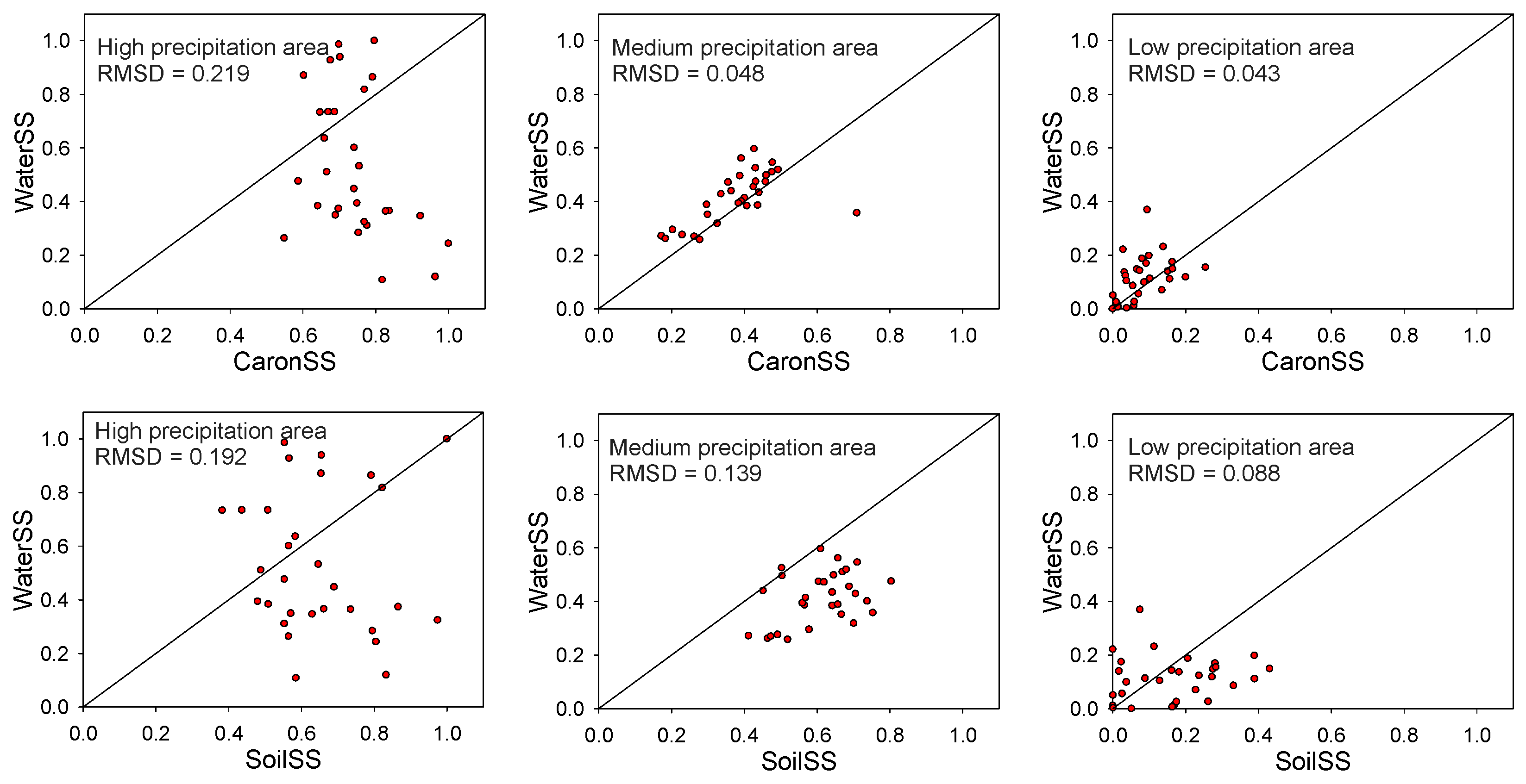
3.2. Characteristics of Changes in Trade-Offs between ESs along the Precipitation Gradient

The size of the trade-off between carbon sequestration and water yield showed a decreasing trend from the high-precipitation area to the medium-precipitation area to the low-precipitation area, but there was no significant difference between medium- and low-precipitation area (Figure 2). The trade-off size between soil conservation and water yield also followed a decreasing trend from the high-precipitation area to the medium-precipitation area to the low-precipitation area, and the difference was significant.
The scatterplot reflects the relative advantage of two ESs supply (Figure 3). For the trade-off between carbon sequestration and water yield, there were more small watersheds (20 small watersheds) that were conducive to carbon sequestration in the high-precipitation area, which was related to the high vegetation coverage. There were more small watersheds that were conducive to water yield in the medium-precipitation area (24 small watersheds) and low precipitation area (17 small watersheds), but the trade-off size was not large, which was 0.048 and 0.043 respectively, and the scatter plots fluctuated around the 1:1 line. For trade-off between soil conservation and water yield, more small watersheds were beneficial to soil conservation in the three precipitation areas, the most serious case was that only one small watershed was beneficial to water yield in the medium-precipitation area, indicating the relative lack of water resources. Thus, it can be seen that the direction of the two trade-off types (carbon sequestration-water yield trade-off and soil conservation-water yield trade-off) was not consistent, which needed to be considered comprehensively in the regulation of ecosystem services.

3.3. The Factors Influencing Ecosystem Services Supply–Demand Balance

For the high-precipitation area, population density had a negative effect on the supply–demand balance of carbon sequestration and the conditional effect was as high as 75. 9%, while NDVI and precipitation had positive effect, but the conditional effects were very low (1.6% and 1.1%) (Table 2). The important impact of population density indicated that the demand side exerted a significant influence on supply–demand relationship. For the medium-precipitation area, soil organic-matter content and the proportion of forest had the greater impact on the supply–demand balance of carbon sequestration (conditional effects were 53.2% and 10.8%, respectively), and population density, NDVI and GDP also had a certain impact (conditional effects were 8.1%, 4.6% and 3.5%, respectively). Because of the positive effects of soil organic matter and forest on carbon sequestration, the above results indicated that the supply side exerted a significant influence on the supply–demand relationship. For the low-precipitation area, the supply–demand balance of carbon sequestration was mainly affected by population density and GDP, and other factors had a very small impact, which indicated that the demand side was dominant in the supply–demand relationship.
The factors influencing soil-conservation supply–demand balance were similar across three precipitation areas. Slope gradient was the dominant factor, and the conditional effects were 46.2%, 40.3% and 95.0% in the high-, medium-, and low-precipitation areas, respectively. Not only soil-conservation supply but also soil-conservation demand was significantly correlated with slope gradient. Other factors, such as precipitation and soil organic-matter content, also had a certain effect on supply–demand balance, but the conditional effects were less than 16%.
For the high-precipitation area, the proportions of grassland and cropland cover had important and positive impacts on the supply–demand balance of water yield (the conditional effects were 49.6% and 18.4%, respectively), and the correlation analysis showed that the two factors were significantly correlated with the supply of water yield, indicating that the supply side was dominant in the supply–demand relationship. Population density had a secondary effect, but the conditional effect was positive. Correlation analysis showed that there was a significant positive correlation between population density and the proportion of cropland cover and a significant negative correlation between population density and the proportion of forest cover. Given the premise of the dominant position of the supply side, the positive effect of population density on the supply–demand balance actually included the role of land-use types. In other words, population density indirectly affects the supply of water yield (positive effect). For the medium-precipitation area, the effects of precipitation, forest cover and shrub cover on the supply–demand balance of water yield were greater and the effects of soil organic matter and grassland were secondary, indicating that the supply side exerted a significant influence on the supply–demand relationship. For the low-precipitation area, the positive effect of precipitation was the largest (conditional effect was 22.3%), followed by the effect of population density, and the conditional effect was negative (13.5%). The direction of influence of population density was different from that in the high-precipitation area. Further analysis found that the correlations between population density and cropland cover and between population density and forest cover were not significant, and the main role of population density was to strengthen the demand for water yield (the correlation coefficient between them was as high as 0.982).

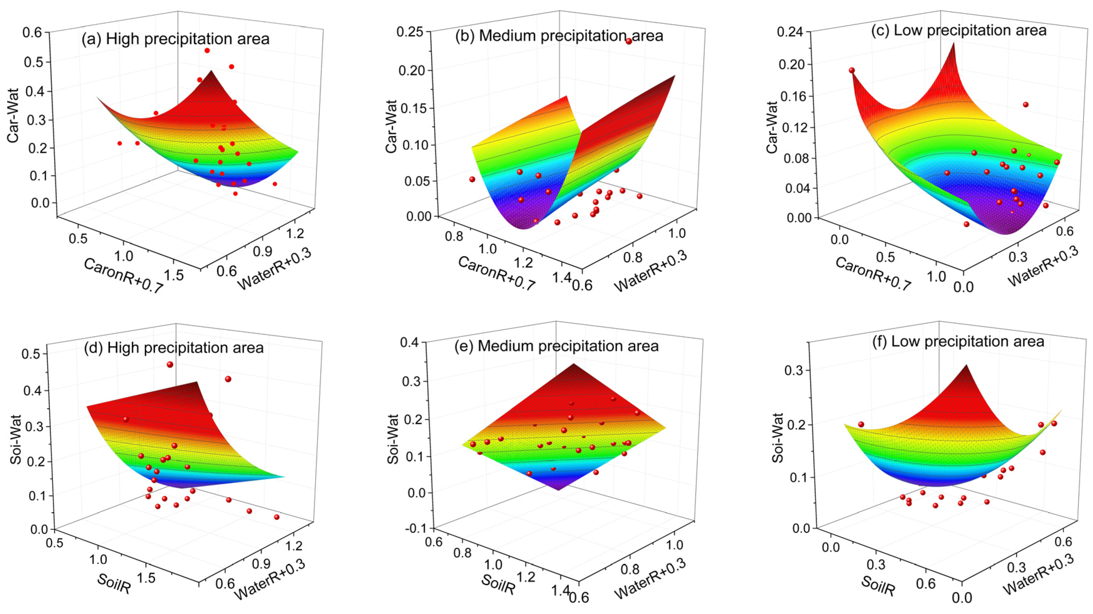
3.4. The Factors Influencing Ecosystem Services Trade-Offs

In the high-precipitation area, the trade-off between carbon sequestration and water yield was mainly affected by the proportion of forest cover (positive effect), and the conditional effect was as high as 69.7% (Table 3). The reason was that forest cover was conducive to carbon sequestration due to photosynthesis but was not conducive to water yield due to evapotranspiration, so the forest ultimately intensified the trade-off. The proportion of grassland cover was the second factor, but the conditional effect was only 9.6%. The role of carbon sequestration and water consumption by grasslands was smaller than the roles of carbon sequestration and water consumption by forests, so grassland cover weakened the trade-off size. In the medium-precipitation area, the trade-off between carbon sequestration and water yield was mainly affected by soil organic-matter content, NDVI and the proportion of forest cover. The correlation analysis showed that carbon sequestration was significantly positively correlated with soil organic-matter content and NDVI; the two factors increased the trade-off size mainly by increasing carbon sequestration. The trade-off between carbon sequestration and water yield was mainly affected by population density (conditional effect was as high as 45.5%) in the low-precipitation area. There was a higher proportion of construction land in the areas with high population density, and carbon sequestration was lower and water yield was higher in these areas; thus, the size of the trade-off between two ESs increased. In addition, precipitation also had a positive effect on size of trade-offs. The correlation coefficient between carbon sequestration and trade-off size was only 0.093 (not significant), and the correlation coefficient between water yield and trade-off size was 0.784 (significant), which indicated that water yield played a leading role in shaping the trade-off. Meanwhile, precipitation was more strongly correlated with water yield than with carbon sequestration. The above results reflect the important effect of precipitation on water yield, and precipitation intensified the trade-offs in the low-precipitation area. The proportion of bare land also played a certain role in influencing trade-off size in the low-precipitation area because bare land reduced carbon sequestration and transpiration at the same time; the factor make trade-offs more significant.
In the high-precipitation area, the trade-off between soil conservation and water yield was mainly affected by the proportion of grassland cover (negative effect), and the conditional effect reached 39.2%. Correlation analysis showed that the proportion of grassland cover was not significantly correlated with soil conservation, but it was significantly positively correlated with water yield. As most small watersheds were conducive to soil conservation (Figure 3), the contribution of grassland cover to water yield reduced the size of the trade-off between soil conservation and water yield. In the medium-precipitation area, the trade-off between soil conservation and water yield was mainly affected by the slope gradient (conditional effect was 39.9%), and the proportion of cropland and grassland cover also had a certain impact (conditional effects of 15.0% and 10.0%, respectively). The process of evaluation of soil conservation was as follows: the difference between the potential soil loss and the actual soil loss was calculated first, and then this difference was revised according to the sediment delivery ratio. The potential soil erosion escalated more rapidly with increasing slope compared to the actual erosion, indicating that soil-conservation services were more significant at steeper inclines. Correlation analysis indicated that slope gradient was significantly positively correlated with soil conservation but not significantly correlated with water yield, which caused slope gradient to exacerbate trade-offs. Similarly, the conditional effect of slope gradient was the largest (24.9%) in the low-precipitation area. The proportion of bare land also had a certain impact. Bare land was not conducive to soil conservation but was prone to runoff (water yield). Since most small watersheds tended towards soil conservation (Figure 3), the proportion of bare land had the effect of weakening trade-offs.

3.5. The Characteristics of the Linkage between Ecosystem-Services Supply–Demand Dynamics and Trade-Offs

The size of the trade-off between carbon sequestration and water yield was taken as the dependent variable, and the supply–demand balance of carbon sequestration and the supply–demand balance of water yield were taken as the independent variables, and surface fitting was implemented. The results are shown in Figure 4 and Table 4. For the high-precipitation area, a quadratic function describes the relationship between carbon-sequestration–water-yield trade-off size and carbon-sequestration–supply–demand balance, the trade-off size first decreased and then increased with the supply–demand balance of carbon sequestration, and the trade-off size was the lowest when the supply-supply ratio was 0.161. There was a logarithmic relationship between carbon-sequestration–water-yield trade-off size and water-yield supply–demand balance, and the trade-off size decreased with increased supply–demand balance. An increase in the supply–demand balance of water yield meant that the negative effects of water consumption were mitigated, so the size of the trade-off between carbon sequestration and water yield was reduced. For the medium-precipitation area, the relationship between carbon-sequestration–water-yield trade-off size and carbon-sequestration supply–demand balance was also described by a quadratic function, and the trade-off size was the lowest when the supply–demand balance was 0.395. There was a power-function relationship between the trade-off size and water-yield–supply–demand balance; the trade-off size increased slowly with the increase in the balance between supply and demand. For the low-precipitation area, the relationship between carbon-sequestration–water-yield trade-off size and carbon-sequestration–supply–demand balance was described by a logarithmic function. The relationship between trade-off size and water-yield supply–demand balance could be described by a quadratic function. Trade-offs were smallest when the supply–demand balance was 0.049. In summary, there was a nonlinear response relationship between carbon-sequestration–water-yield trade-off size and the supply–demand balance of each ES. There was often a critical point in the response of the trade-off size to the supply–demand balance; when supply–supply ratio reached a certain level, the trade-off was smallest, which provided a possible route for the comprehensive regulation of trade-offs and supply–demand dynamics.
For the high-precipitation area, the relationship between the trade-off between soil conservation and water yield and the soil-conservation supply–demand balance could be described by a linear function, and the trade-off size increased with the increase of supply–demand balance. However, the relationship between the size of the trade-off between soil conservation and water yield and the water-yield supply–demand balance could be described by a reciprocal function, and the trade-off size decreased with increased supply–demand balance. For the medium-precipitation area, a linear function described the relationship between size of the trade-off between soil conservation and water yield and the supply–demand balance of the two services. Trade-off size increased with the supply–demand balance of soil-conservation services, but trade-off size decreased with the supply–supply ratio of water yield. For the low-precipitation area, a quadratic function described the relationship between the size of the trade-off between soil conservation and water yield and the soil-conservation supply–demand balance, and trade-off size was the lowest when soil-conservation supply–demand balance was 0.081. Similarly, when water-yield supply–demand balance was 0.169, the trade-off size was the lowest.
The coefficient of determination indicates the degree to which the characteristics of the correlation between supply–demand dynamics and trade-offs were fitted. Based on the results in Table 2, Table 3 and Table 4, it could be observed that the correlation between trade-offs and balance between supply and demand was influenced by various natural and human factors. When the trade-off size and supply–demand balance were controlled by similar factors, the correlation between them was stronger and R2 was larger. On the contrary, when there were differences in the main factors controlling trade-off size and supply–demand balance, the correlation between them was weak and R2 was small. For example, in the high-precipitation area, the main factors controlling the Car-Wat trade-off and supply–demand balance for both ESs were indicators of population density and vegetation cover, so R2 was larger (0.8019). In the medium-precipitation area, soil organic matter and vegetation cover were the main factors controlling the Car-Wat trade-off and caronR, but a new index, precipitation, was the main factor controlling WaterR, which led to a weak correlation between trade-off and balance between supply and demand, so R2 was smaller (0.4029).

4. Discussion

4.1. Spatial Differentiation of ESs in Different Geographical Spaces

ESs tend to be regularly distributed across topographic and climatic gradients; for example, the ratios of supply to demand for various ESs in the Lancang River Basin were low in the upper reaches and high in the lower reaches, a pattern similar to the distribution trends of topography and climate [34]. Water yield, soil carbon sequestration and hydrological regulation increased with precipitation in the Loess Plateau, but understory plant diversity did not show this trend [26,35,36]. In addition, the correlation between ESs supply and social demand in most dryland areas strengthens with increased precipitation in the Loess Plateau [37]. Wang et al. found that the trade-off between soil moisture and total nitrogen became larger as precipitation increased, but the trade-off between soil moisture and organic matter first increased and then decreased with increasing precipitation in the Loess Plateau [26]. Similarly, Feng et al. found that the trade-off between water yield and carbon sequestration first increased and then decreased with increasing precipitation, but that between water yield and soil conservation first decreased and then increased in the central Loess Plateau [27]. In this study, the supply, supply–demand balance and trade-off size of the three ESs increased with increasing precipitation, but the demand for ESs did not show a consistent trend (Figure 2). Therefore, there is regional differentiation in ESs with the environmental gradient, but due to the different ESs types, regional characteristics and estimation methods, the gradient trends are diverse.

4.2. Diversity of Factors Affecting Supply, Demand and Trade-Offs of ESs

The supply of ESs is affected by vegetation cover, rainfall, topography, soil and other natural factors [38,39]. There are differences in the direction, speed and degree of the response of ESs to different factors, which is one of the reasons for the trade-offs between different ESs [40]. Revealing the key determinants of trade-offs provides a possible way to coordinate different ESs. In this study, we found that the trade-off between carbon sequestration and water yield was predominantly influenced by the proportion of forest and grassland cover and by soil organic matter in the medium- and high-precipitation areas, while the size of the trade-off in the low-precipitation area was mainly controlled by population density and precipitation, and bare land also had a certain impact. The size of the trade-off between soil conservation and water yield was affected by the proportion of grassland cover in the high-precipitation area, while it was mainly controlled by the slope gradient in the low-precipitation area. The above results are similar to those of previous studies; Feng et al. found that the proportions of forest and grassland cover played a leading role in the trade-off between carbon sequestration and water yield, while the slope gradient and the proportion of grassland cover played a leading role in shaping the trade-off between soil conservation and water yield in the Ansai watershed in the Loess Plateau [21]. In addition, Feng et al. also found that an increased proportion of forest cover increased the size of the trade-off in three watersheds with different degrees of precipitation, but grassland cover reduced the size of the trade-offs in the middle-precipitation (mean annual precipitation greater than 400 mm but less than 500 mm) and high-precipitation (mean annual precipitation greater than 500 mm but less than 600 mm) watersheds, and grassland cover increased the size of the trade-offs in the low-precipitation (mean annual precipitation greater than 300 mm but less than 400 mm) watershed [27]. Therefore, the effects of land-use design and physiographic conditions need to be considered in the resolution of conflicts between ESs in the Loess Plateau.
The supply of ESs is mainly affected by natural factors, and the demand for ESs is affected by economic and social determinants like population density and GDP [41,42], so the supply–demand balance of ESs is affected by both natural and socio-economic factors [43,44]. However, the dominant factors affecting supply–demand balance are different in different geographical environments, a result that presents important references for the regulation of the supply–demand relationships of ESs. One study in the Huaihe River Basin found that supply–demand balance was mainly affected by social and economic factors, with natural factors being a secondary influence. Ecological land cover increased the balance between supply and demand, but construction land cover decreased the balance between supply and demand [45]. However, Yang et al. found that matching between the supply and demand for ESs in the whole Loess Plateau was mainly affected by natural factors such as vegetation, with socio-economic factors being a secondary influence [37]. Li found that the balance between supply and demand for carbon sequestration was mainly positively affected by NDVI, precipitation and potential evapotranspiration and was negatively affected by human disturbance (GDP and population density); the supply–demand balance of soil conservation was mainly positively affected by topography and NDVI, and negatively affected by potential evapotranspiration; the supply–demand balance of water yield was mainly positively affected by precipitation [30]. The results of this study are similar to those of previous studies: the primary factors affecting the supply–demand balance of carbon sequestration in the high-, medium- and low-precipitation areas are population density, soil organic-matter content, and population density, respectively; the principal determinants affecting the supply–demand balance of water yield are grassland cover, forest cover, and precipitation, respectively; the principal determinant affecting the supply–demand balance of soil conservation in the three precipitation areas is slope gradient. Therefore, the characteristics of trade-offs, supply–demand balance and their influencing factors in different geographical areas need to be considered as a whole in the ecological restoration of territorial spaces.

4.3. The Intrinsic Mechanism of the Correlation between Supply–Demand Dynamics and Trade-Offs in ESs

On the one hand, the trade-off between ESs means the reduction in one of the services, which may result in a conflict between supply and demand owing to a lack of adequate provision for this service; on the other hand, when the supply of a service (such as food supply) is insufficient, people take measures (such as deforestation and land reclamation) to increase the service, however, this could result in heightened soil erosion and induce a trade-off between the provision of food and the preservation of soil. Therefore, the correlation between supply–demand dynamics and trade-offs is logically valid [40]. This study found that there was indeed a certain degree of correlation between supply–demand dynamics and trade-offs (Figure 4 and Table 4), and the dominant factors affecting supply–demand dynamics and trade-offs are often similar. For example, the main factors affecting the carbon-sequestration supply–demand balance, the water-yield supply–demand balance, and the size of the trade-off between carbon sequestration and water yield are similar in the low-precipitation area (population density, precipitation, etc.) (Table 2 and Table 3). This is the intrinsic reason for the correlation between supply–demand dynamics and trade-offs. However, there were also differences in the primary factors influencing supply–demand dynamics and trade-offs. For example, the supply–demand balance of soil conservation in the medium-precipitation area was mainly affected by slope gradient and soil organic matter, while the supply–demand balance of water yield was mainly affected by precipitation and the proportion of forest and grassland, but the trade-off between the two ESs was affected by a new factor (the proportion of cropland) in addition to these factors. Consequently, some factors affect supply–demand dynamics and trade-offs at the same time, while others have a greater effect on either supply–demand balance or trade-offs, which provides a possible mechanism for joint and targeted regulation and is conducive to the synchronous resolution of conflicts over ESs and supply–demand imbalances [40].
Due to the diversity of and similarities and differences between the factors influencing supply–demand dynamics and trade-offs, the characteristics of the correlation between supply–demand dynamics and trade-off sizes are relatively complex, described by a non-linear response relationship (Figure 4). In this study, a quadratic function describes the relationship between the trade-off between carbon sequestration and water yield and the supply–demand balances of carbon sequestration and water yield in the three precipitation areas, and there is a threshold of supply–demand balance to minimize the trade-off size. Meanwhile, a quadratic function describes the relationship between the trade-off between soil conservation and water yield and the supply–demand balance of soil conservation and water yield in the low-precipitation area, and there is also a threshold of supply–demand balance to minimize the trade-off size. The response curve (function) is helpful for developing a full understanding of the characteristics of the correlation between trade-off and supply–demand balance, which provides a new mechanism for the synchronous resolution of conflicts over services and supply–demand imbalance.

4.4. The Limitations of this Study and Prospective Future Studies

In this study, the catchment as a whole was used as a research sample to analyze the characteristics of the correlation between supply–demand dynamics and trade-offs in ESs, and this study provides a reference for ESs management at the catchment scale in areas with different degrees of precipitation. We considered only a single time node and did not analyze the spatial variation of supply–demand dynamics and trade-off associations in small watersheds. The impact of ESs flows on the supply–demand relationship was neglected. Future research should integrate trade-off, flow, supply–demand matching and residents’ well-being with regard to ESs and systematically reveal the characteristics of the correlations between supply–demand dynamics, trade-offs and well-being effects.

5. Conclusions

The supply of carbon sequestration, soil conservation, and water yield, as well as the supply–demand balance for these three ESs, all exhibited a decreasing trend from the high-precipitation area to the medium-precipitation area to the low-precipitation area. However, the demand for these three ESs did not show a consistent pattern. The trade-off between carbon sequestration and water yield, as well as that between soil conservation and water yield, all showed a decreasing trend from the high-precipitation area to the medium-precipitation area to the low-precipitation area. The tendencies of trade-offs between carbon sequestration and water yield, and between soil conservation and water yield, were not consistent.
The supply–demand balance of carbon sequestration was primarily influenced by population density, soil organic-matter content, and population density in the high-, medium- and low-precipitation areas, respectively. The dominant factor affecting the supply–demand balance of soil conservation in the three precipitation areas was slope gradient. The supply–demand balance of water yield was primarily influenced by the grassland cover, forest cover, and precipitation in the three precipitation areas. The primary factors influencing the trade-offs between carbon sequestration and water yield in high-, medium- and low-precipitation areas were forest cover, soil organic-matter content, and population density, respectively, and those influencing the size of the trade-off between soil conservation and water yield in the three precipitation areas were grass proportion, slope gradient and slope gradient, respectively.
The relationships between the supply–demand dynamics and the sizes of the trade-offs in ESs were often nonlinear. Firstly, a quadratic relationship was the most common; this relationship includes a threshold value of the supply–demand balance that minimized the trade-off size. Secondly, there was a monotonic nonlinear relationship, in which the trade-off size increased or decreased unevenly as the supply–demand balance increased. Finally, there was also a linear relationship between the trade-off and the supply–demand balance.
This study revealed the factors influencing ESs supply–demand dynamics and trade-off sizes in areas with different levels of precipitation and the characteristics of their correlations; the results provide a new mechanism for the simultaneous regulation of conflicts over ESs and supply–demand imbalance.

Author Contributions

Project administration, writing—original draft preparation, Q.F.; writing—review and editing, B.D.; investigation and data curation, X.Z. All authors have read and agreed to the published version of the manuscript.

Funding

This research was funded by the Humanities and Social Science Fund of Ministry of Education of China (No. 22YJAZH018) and the Fundamental Research Program of Shanxi Province (No. 20210302123481) and the State Key Laboratory of Earth Surface Processes and Resource Ecology (No. 2022-KF-02).

Data Availability Statement

The data presented in this study are available on request from the corresponding author. The data are not publicly available due to restrictions on non-public data from governments and research institutions.

Conflicts of Interest

The authors declare no conflicts of interest.

References

  1. Costanza, R.; D’Arge, R.; de Groot, R.; Farber, S.; Grasso, M.; Hannon, B.; Limburg, K.; Naeem, S.; O’Neill, R.V.; Paruelo, J.; et al. The Value of the World’s Ecosystem Services and Natural Capital. Nature 1997, 387, 253–260. [Google Scholar] [CrossRef]
  2. Millennium Ecosystem Assessment. Ecosystem and Human Well-Being; Island Press: Washington, DC, USA, 2005; pp. 137–142. [Google Scholar]
  3. Bennett, E.M.; Peterson, G.D.; Gordon, L.J. Understanding Relationships among Multiple Ecosystem Services. Ecol. Lett. 2009, 12, 1394–1405. [Google Scholar] [CrossRef] [PubMed]
  4. Matsuzaki, S.S.; Kohzu, A.; Kadoya, T.; Watanabe, M.; Osawa, T.; Fukaya, K.; Komatsu, K.; Kondo, N.; Yamaguchi, H.; Ando, H.; et al. Role of wetlands in mitigating the trade-off between crop production and water quality in agricultural landscapes. Ecosphere 2019, 10, e02918. [Google Scholar] [CrossRef]
  5. Segre, H.; Carmel, Y.; Shwartz, A. Economic and not ecological variables shape the sparing–sharing trade-off in a mixed cropping landscape. J. Appl. Ecol. 2022, 59, 779–790. [Google Scholar] [CrossRef]
  6. Biel, R.G.; Hacker, S.D.; Ruggiero, P. Coastal protection and conservation on sandy beaches and dunes: Context-dependent tradeoffs in ecosystem service supply. Ecosphere 2017, 8, e01787. [Google Scholar] [CrossRef]
  7. Mouchet, M.; Lamarque, P.; Martín-López, B. An Interdisciplinary Methodological Guide for Quantifying Associations between Ecosystem Services. Glob. Environ. Change 2014, 28, 298–308. [Google Scholar] [CrossRef]
  8. Cortinovis, C.; Geneletti, D. A performance-based planning approach integrating supply and demand of urban ecosystem services. Landsc. Urban Plan. 2020, 201, 103842. [Google Scholar] [CrossRef]
  9. Kroll, F.; Mueller, F.; Haase, D.; Fohrer, N. Rural-urban gradient analysis of ecosystem services supply and demand dynamics. Land Use Policy 2012, 29, 521–535. [Google Scholar] [CrossRef]
  10. Arnaiz-Schmitz, C.; Herrero-Jáuregui, C.; Schmitz, M.F. Recreational and nature-based tourism as a cultural ecosystem service: Assessment and mapping in a rural-urban gradient of central Spain. Land 2021, 10, 343. [Google Scholar] [CrossRef]
  11. Lu, N.; Liu, L.; Yu, D. Navigating trade-offs in the social-ecological systems. Curr. Opin. Environ. Sustain. 2021, 48, 77–84. [Google Scholar] [CrossRef]
  12. Neyret, M.; Fischer, M.; Allan, E. Assessing the Impact of Grassland Management on Landscape Multifunctionality. Ecosyst. Serv. 2021, 52, 101366. [Google Scholar] [CrossRef]
  13. Tan, J.; Peng, L.; Wu, W.; Huang, Q. Mapping the evolution patterns of urbanization, ecosystem service supply–demand, and human well-being: A tree-like landscape perspective. Ecol. Indic. 2023, 154, 110591. [Google Scholar] [CrossRef]
  14. Zheng, H.; Wang, L.J.; Wu, T. Coordinating ecosystem service trade-offs to achieve win–win outcomes: A review of the approaches. J. Environ. Sci. 2019, 82, 103–112. [Google Scholar] [CrossRef] [PubMed]
  15. Li, X.; Yu, X.; Wu, K.N. Land-use zoning management to protect the regional key ecosystem services: A case study in the city belt along the Chaobai River, China. Sci. Total Environ. 2020, 762, 143167. [Google Scholar] [CrossRef] [PubMed]
  16. Wang, L.J.; Zheng, H.; Wen, Z. Ecosystem service synergies/trade-offs informing the supply-demand match of ecosystem services: Framework and application. Ecosyst. Serv. 2019, 37, 100939. [Google Scholar] [CrossRef]
  17. Zhang, H.; Zhang, Z.; Liu, K.; Huang, C.; Dong, G. Integrating land use management with trade-offs between ecosystem services: A framework and application. Ecol. Indic. 2023, 149, 110193. [Google Scholar] [CrossRef]
  18. Fang, G.; Sun, X.; Sun, R.; Liu, Q.; Tao, Y.; Yang, P.; Tang, H. Advancing the optimization of urban–rural ecosystem service supply–demand mismatches and trade-offs. Landscape Ecol. 2024, 39, 32. [Google Scholar] [CrossRef]
  19. Bottalico, F.; Pesola, L.; Vizzarri, M.; Antonello, L.; Barbati, A.; Chirici, G.; Corona, P.; Cullotta, S.; Garfi, V.; Giannico, V.; et al. Modeling the influence of alternative forest management scenarios on wood production and carbon storage: A case study in the Mediterranean region. Environ. Res. 2016, 144, 72–87. [Google Scholar] [CrossRef] [PubMed]
  20. Kim, M.; Kraxner, F.; Forsell, N.; Song, C.; Lee, W.K. Enhancing the provisioning of ecosystem services in South Korea under climate change: The benefits and pitfalls of current forest management strategies. Reg. Environ. Change 2021, 21, 6. [Google Scholar] [CrossRef]
  21. Feng, Q.; Zhao, W.W.; Hu, X.P. Trading-off ecosystem services for better ecological restoration: A case study in the Loess Plateau of China. J. Clean. Prod. 2020, 257, 120469. [Google Scholar] [CrossRef]
  22. Hu, B.; Zhang, Z.; Han, H. The Grain for Green Program intensifies trade-offs between ecosystem services in midwestern Shanxi, China. Rem. Sens. 2021, 13, 3966. [Google Scholar] [CrossRef]
  23. Feng, X.M.; Fu, B.J.; Piao, S.L. Revegetation in China’s Loess Plateau is approaching sustainable water resource limits. Nat. Clim. Change 2016, 6, 1019–1022. [Google Scholar] [CrossRef]
  24. Chen, Y.P.; Wang, K.B.; Lin, Y.S. Balancing green and grain trade. Nat. Geosci. 2015, 8, 739–741. [Google Scholar] [CrossRef]
  25. Zhang, Y.; Huang, M.; Lian, J. Spatial distributions of optimal plant coverage for the dominant tree and shrub species along a precipitation gradient on the central Loess Plateau. Agric. For. Meteorol. 2015, 206, 69–84. [Google Scholar] [CrossRef]
  26. Wang, C.; Wang, S.; Fu, B.; Li, Z.; Wu, X.; Tang, Q. Precipitation gradient determines the tradeoff between soil moisture and soil organic carbon, total nitrogen, and species richness in the Loess Plateau, China. Sci. Total Environ. 2017, 575, 1538. [Google Scholar] [CrossRef] [PubMed]
  27. Feng, Q.; Dong, S.Y.; Duan, B.L. The effects of land-use change/conversion on trade-offs of ecosystem services in three precipitation zones. Sustainability 2021, 13, 13306. [Google Scholar] [CrossRef]
  28. Jian, Z.; Sun, Y.; Wang, F.; Zhou, C.; Pan, F.; Meng, W.; Sui, M. Soil conservation ecosystem service supply-demand and multi-scenario simulation in the Loess Plateau, China. Glob. Ecol. Conserv. 2024, 49, e02796. [Google Scholar] [CrossRef]
  29. Ma, Y.; Chen, H.; Liu, D.; Zhang, J.; Yang, M.; Shi, J. Identification and management of priority regulation areas based on the supply–demand relationship of ecosystem services: A case study of the Loess Plateau. Ecol. Indic. 2024, 159, 111754. [Google Scholar] [CrossRef]
  30. Li, J. Identification of ecosystem services supply and demand and driving factors in Taihu Lake Basin. Environ. Sci. Pollut. Res. 2022, 29, 29735–29745. [Google Scholar] [CrossRef]
  31. Sharp, R.; Tallis, H.T.; Ricketts, T.; Guerry, A.D.; Wood, S.A.; Chaplin-Kramer, R. InVEST + VERSION User’s Guide; The Natural Capital Project, Stanford University: Stanford, CA, USA; University of Minnesota: Minneapolis, MN, USA; The Nature Conservancy: Arlington County, VA, USA; World Wildlife Fund: Palo Alto, CA, USA, 2016; pp. 115–120. [Google Scholar]
  32. Bradford, J.B.; D’Amato, A.W. Recognizing trade-offs in multi-objective land management. Front. Ecol. Environ. 2012, 10, 210–216. [Google Scholar] [CrossRef]
  33. Li, J.; Bai, Y.; Alatalo, J.M. Impacts of rural tourism-driven land use change on ecosystems services provision in Erhai Lake Basin, China. Ecosyst. Serv. 2020, 42, 101081. [Google Scholar] [CrossRef]
  34. Liu, S.; Sun, Y.; Wu, X.; Li, W.; Liu, Y.; Tran, L.S.P. Driving factor analysis of ecosystem service balance for watershed management in the Lancang River Valley, Southwest China. Land 2021, 10, 522. [Google Scholar] [CrossRef]
  35. Lü, Y.; Fu, B.; Feng, X.; Zeng, Y.; Liu, Y.; Chang, R. A policy-driven large scale ecological restoration: Quantifying ecosystem services changes in the Loess Plateau of China. PLoS ONE 2012, 7, e31782. [Google Scholar] [CrossRef]
  36. Lu, N.; Fu, B.; Jin, T.; Chang, R. Trade-off analyses of multiple ecosystem services by plantations along a precipitation gradient across Loess Plateau landscapes. Landscape Ecol. 2014, 29, 1697–1708. [Google Scholar] [CrossRef]
  37. Yang, M.H.; Zhao, X.N.; Wu, P.; Hu, P.; Gao, X.D. Quantification and spatially explicit driving forces of the incoordination between ecosystem service supply and social demand at a regional scale. Ecol. Indic. 2022, 137, 108764. [Google Scholar] [CrossRef]
  38. Braun, D.; Jong, R.; Schaepman, M.E.; Furrer, R.; Hein, L.; Kienast, F.; Damm, A. Ecosystem service change caused by climatological and non-climatological drivers: A Swiss case study. Ecol. Appl. 2019, 29, e01901. [Google Scholar] [CrossRef] [PubMed]
  39. Bai, Y.; Ochuodho, T.O.; Yang, J. Impact of land use and climate change on water-related ecosystem services in Kentucky, USA. Ecol. Indic. 2019, 102, 51–64. [Google Scholar] [CrossRef]
  40. Feng, Q.; Zhao, W.W.; Duan, B.L.; Hu, X.P.; Cherubini, F. Coupling trade-offs and supply-demand of ecosystem services (ES): A new opportunity for ES management. Geogr. Sustain. 2021, 2, 275–280. [Google Scholar] [CrossRef]
  41. Lorilla, R.S.; Poirazidis, K.; Detsis, V.; Kalogirou, S.; Chalkias, C. Socio-ecological determinants of multiple ecosystem services on the Mediterranean landscapes of the Ionian Islands (Greece). Ecol. Model. 2020, 422, 108994. [Google Scholar] [CrossRef]
  42. Zhang, J.; Guo, W.; Tang, Z.; Qi, L. Identifying the regional spatial management of ecosystem services from a supply and demand perspective: A case study of Danjiangkou reservoir area, China. Ecol. Indic. 2024, 158, 111421. [Google Scholar] [CrossRef]
  43. Wei, H.; Fan, W.; Wang, X.; Lu, N.; Dong, X.; Zhao, Y. Integrating supply and social demand in ecosystem services assessment: A review. Ecosyst. Serv. 2017, 25, 15–27. [Google Scholar] [CrossRef]
  44. Xia, F.; Yang, Y.; Zhang, S.; Li, D.; Sun, W.; Xie, Y. Influencing factors of the supply-demand relationships of carbon sequestration and grain provision in China: Does land use matter the most? Sci. Total Environ. 2022, 832, 154979. [Google Scholar] [CrossRef]
  45. Zhuang, Z.; Li, C.; Hsu, W.L.; Gu, S.; Hou, X.; Zhang, C. Spatiotemporal changes in the supply and demand of ecosystem services in China’s Huai River Basin and their influencing factors. Water 2022, 14, 2559. [Google Scholar] [CrossRef]
Figure 1. The location of the study area.
Land 13 01057 g001
Figure 2. The significant differences in ESs supply, demand, supply–demand balance and trade-off among three precipitation areas (Note: The lower-case letters on the bars represent the significance of the difference (p < 0.05) among different precipitation areas. CaronS: carbon-sequestration supply, SoilS: soil-conservation supply, WaterS: water-yield supply, CaronD: carbon-sequestration demand, SoilD: soil-conservation demand, WaterD: water-yield demand, CaronR: supply–demand balance of carbon sequestration, SoilR: supply–demand balance of soil conservation, WaterR: supply–demand balance of water yield, Car-Wat: size of the trade-off between carbon sequestration and water yield, Soi-Wat: size of the trade-off between soil conservation and water yield. The below is the same).
Land 13 01057 g002
Figure 3. The relative advantage of two ESs supply(CaronSS, SoilSS and WaterSS represent the normalized values of carbon-sequestration, soil-conservation and water-yield supply respectively).
Land 13 01057 g003
Figure 4. Surface-fitting relationship between ESs trade-off size and supply–demand balance (We add 0.7 and 0.3 to the independent variables CaronR and WaterR, respectively, to ensure their values are positive in order to establish a possible logarithmic relationship. The below is the same.).
Land 13 01057 g004
Table 1. The equations for calculation of the supply and demand for ESs.
ESsAlgorithmsDescription
WaterSWaterSx = (1 − AETx/Px)·PxWaterSx is the water yield on pixel x, AETx is actual evapotranspiration and Px is precipitation. The calculations of AETx are key content, and the InVEST User’s Guide provides the detailed methodology for the calculations [31].
SoilSSoilSx = Rx·Kx·LSx(1 −·Cx·Px)SDRi
+Tx
SoilSx is the total sediment retention (reduction in sediment exported to streams) provided by pixel x from both on-pixel and upslope erosion sources; Rx is rainfall erosivity on pixel x; Kx is the soil erodibility; LSx is a topographical factor; Cx is the cover-management factor; and Px is an engineering measure factor. SDRi is the sediment delivery ratio; Ti is the amount of upslope sediment that is trapped on pixel x.
CaronSCaronSx = APARx × εxCaronSx is the net primary productivity on pixel x; APARx represents the photosynthetically active radiation on pixel x; and εx is the light-use efficiency.
WaterDWaterD = Dind + Dagr + Ddom + DecoWaterD is the demand for water-yield services, Dind, Dagr, Ddom and Deco are the water consumption in industry, agriculture, domestic use, and ecological use, respectively.
SoilDSoilDx = Rx·Kx·LSx·Cx·Px·SDRiSoilDx is sediment export from pixel x that actually reaches a stream; the other parameters are the same as above.
CaronDCaronDx = ρx·φxCaronDx is the carbon-sequestration demand (carbon emissions) on pixel x; φx is the per capita carbon emissions calculated from energy consumption data; and ρx is the density of population.
CaronS: carbon-sequestration supply, SoilS: soil-conservation supply, WaterS: water-yield supply, CaronD: carbon-sequestration demand, SoilD: soil-conservation demand, WaterD: water-yield demand.
Table 2. The conditional effects of driving factors on balance between supply and demand with regard to ecosystem services.
High-Precipitation AreaMedium-Precipitation AreaLow-Precipitation Area
FactorsExplains %pFactorsExplains %pFactorsExplains %p
CaronRPopD75.90.002SOM53.20.002PopD54.50.002
NDVI1.60.022Fore10.80.018GDP17.30.002
Prec1.10.034PopD8.10.006Gras4.20.05
NDVI4.60.026
GDP3.50.036
SoilRSloG46.20.002SloG40.30.002SloG950.002
Prec14.70.002SOM160.004
Fore7.50.008Fore7.20.028
NDVI3.30.034NDVI4.20.096
SOM2.30.02
WaterRGras49.60.002Prec33.80.004Prec22.30.002
Crop18.40.002Fore36.60.002PopD13.50.002
PopD13.10.006Shru14.80.002Bare50.004
Prec3.10.048SOM6.60.002GDP1.50.008
SOM2.90.014Gras1.50.036Fore10.022
(Note: Percentages with gray shadows represent negative effects, and the other values represent positive effects. PopD: population density, NDVI: normalized vegetation index, Prec: precipitation, SloG: slope gradient, Fore: proportion of forest cover, SOM: soil organic-matter content, Gras: proportion of grassland cover, Crop: proportion of cropland cover, Shru: proportion of shrubland cover, GDP: gross domestic product, Bare: bare land. The below is the same).
Table 3. The conditional effects of factors driving ecosystem-services trade-offs.
High-Precipitation AreaMedium-Precipitation AreaLow-Precipitation Area
FactorsExplains %pFactorsExplains %pFactorsExplains %p
Car-WatFore69.70.002SOM48.70.008PopD45.50.01
Gras9.60.006NDVI12.60.004Prec13.80.008
PopD2.10.036Fore8.20.012Bare12.50.026
Soi-WatGras39.20.002SloG39.90.002SloG24.90.002
Crop150.004Bare17.30.008
Gras100.008PopD10.40.018
Table 4. The functional relationship between ESs trade-off size and supply–demand balance.
Precipitation AreaRegression EquationR2p
HCar-Wat = 0.335 − 0.584(CaronR + 0.7) + 0.339(CaronR +0.7)2 −0.432 ln(WaterR + 0.3)0.8019<0.001
MCar-Wat = −1.927 − 2.924(CaronR +0.7) + 1.335(CaronR +0.7)2 + 3.567(WaterR + 0.3)0.0210.4029<0.001
LCar-Wat = 0.116 − 0.028 ln(CaronR +0.7) −0.621(WaterR + 0.3) + 0.890(WaterR + 0.3)20.7117<0.001
HSoi-Wat = −0.319 + 0.112 SoilR + 0.332/(WaterR + 0.3)0.5098<0.001
MSoi-Wat = 0.240 + 0.390 SoilR − 0.596(WaterR + 0.3)0.9593<0.001
LSoi-Wat = 0.268−0.056 SoilR + 0.346 SoilR2 − 0.938(WaterR + 0.3) + (WaterR + 0.3)20.5784<0.001
Disclaimer/Publisher’s Note: The statements, opinions and data contained in all publications are solely those of the individual author(s) and contributor(s) and not of MDPI and/or the editor(s). MDPI and/or the editor(s) disclaim responsibility for any injury to people or property resulting from any ideas, methods, instructions or products referred to in the content.

