
A Model to Analyze Industrial Clusters to Measure Land Use Efficiency in China


Abstract
:1. Introduction
2. Literature Review
3. Materials and Methods
3.1. Analytical Framework
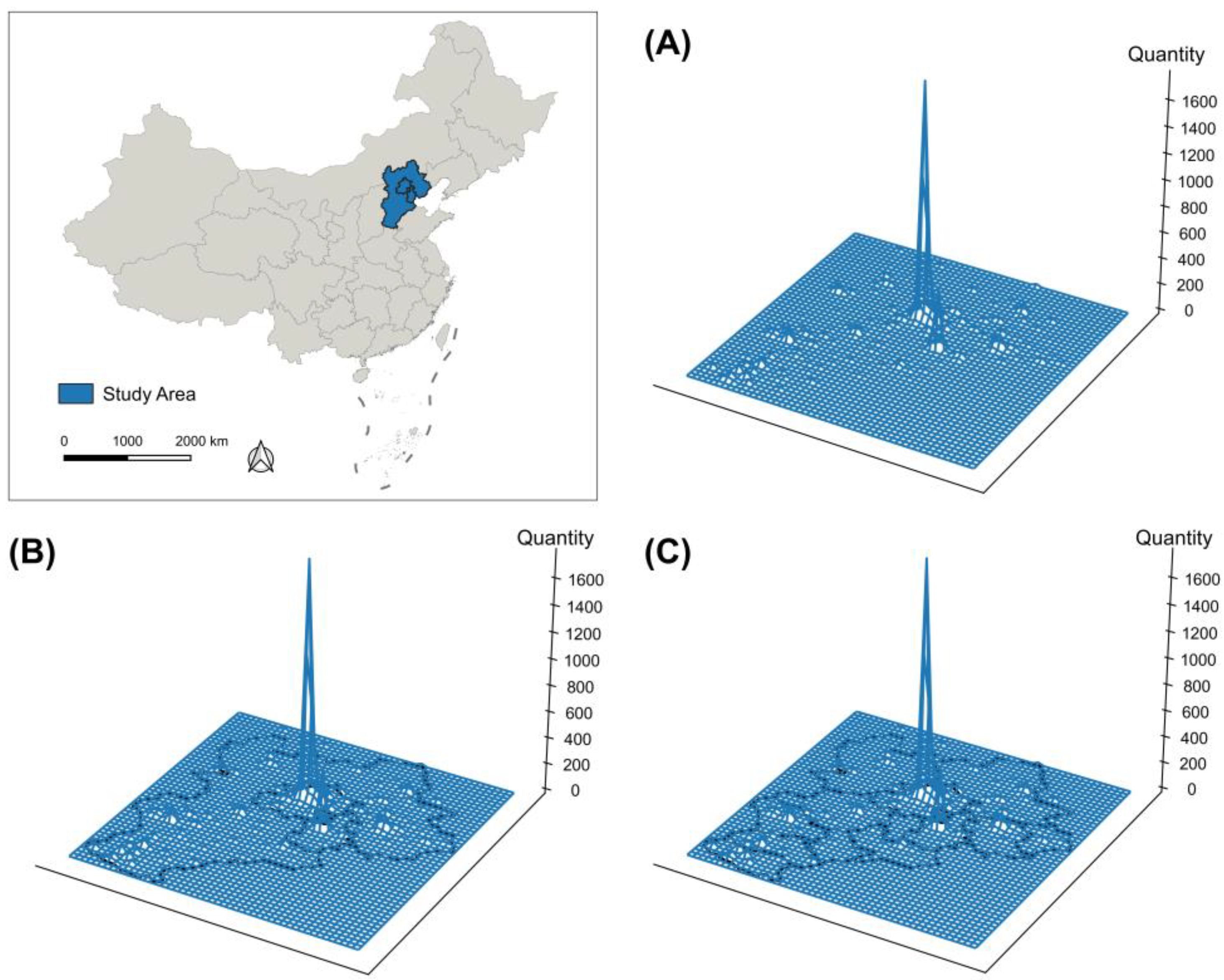
3.2. Study Area and Data
3.3. Methodology
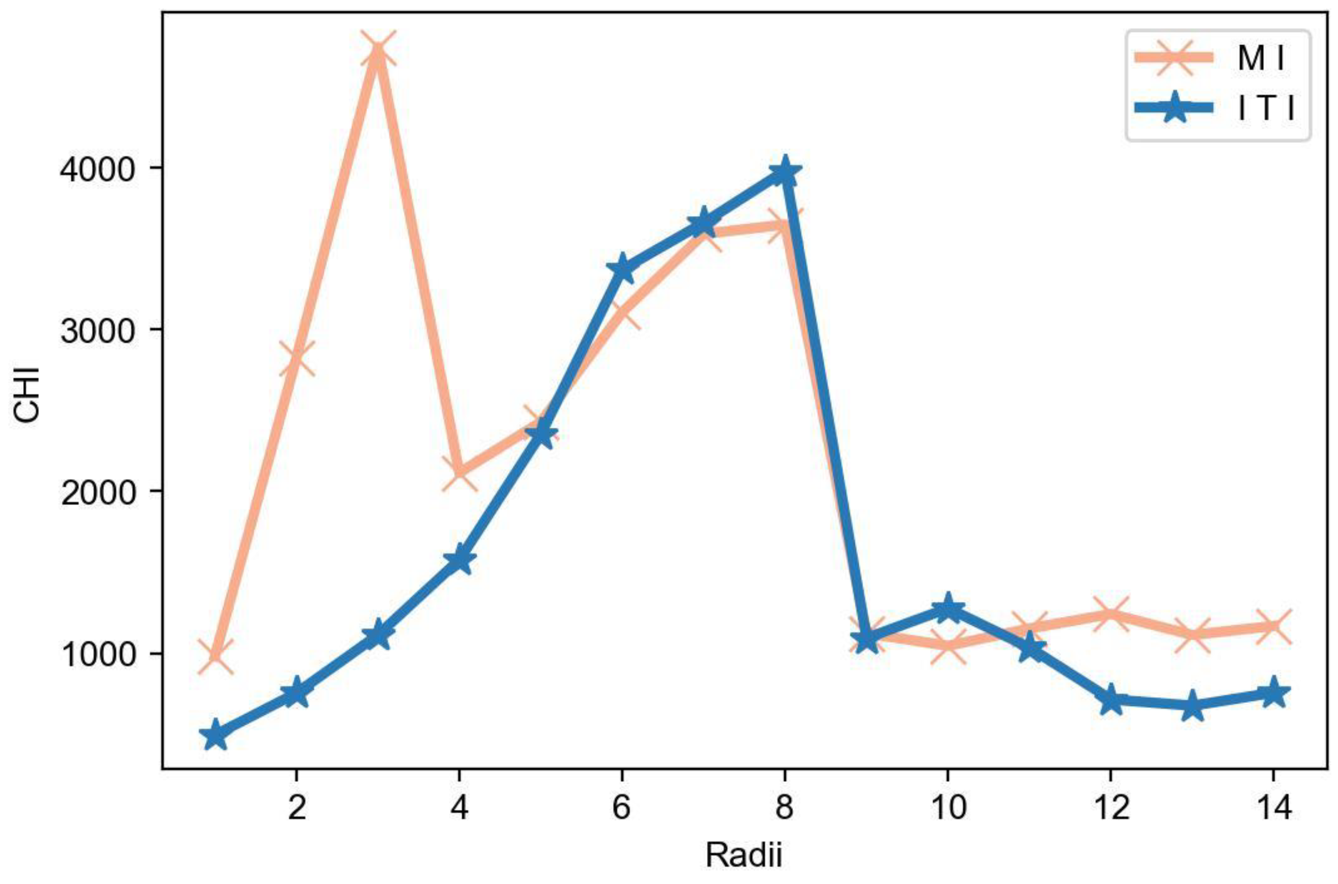
3.3.1. DBSCAN
| Algorithm 1 DBSCAN algorithm | |
| Input: DB: Database | |
| Input: : Radius | |
| Input: : Density threshold | |
| Input: dist: Distance function | |
| Data: label: Point labels, initially undefined | |
| 1 | foreach point p in database DB do |
| 2 | if label(p) ≠ undefined then continue |
| 3 | Neighbors N ← RangeQuery(DB, dist, p, ) |
| 4 | if |N| < then |
| 5 | label(p) ← Noise |
| 6 | continue |
| 7 | c ← next cluster label |
| 8 | label(p) ← c |
| 9 | Seed set S ← N\{p} |
| 10 | foreach q in S do |
| 11 | if label(q) = Noise then label(q) ← c |
| 12 | if label(q) ≠ undefined then continue |
| 13 | Neighbors N ← RangeQuery(DB, dist, q, ) |
| 14 | label(q) ← c |
| 15 | if |N| < then continue |
| 16 | S ← S ∪ N |
3.3.2. Identification of the Spatial Form of Industrial Cluster
3.3.3. Data Envelopment Analysis (DEA)
3.3.4. Spatial Correlation Analysis between Clusters
3.3.5. Spatial Error Model
3.3.6. Spatial Autoregressive Model
4. Results
4.1. Identification of Industrial Clusters
4.2. The Efficiency of Input and Output in Industrial Clusters and Land Use
5. Discussion
5.1. Characteristics of Industrial Clusters
5.1.1. Density of Industrial Clusters
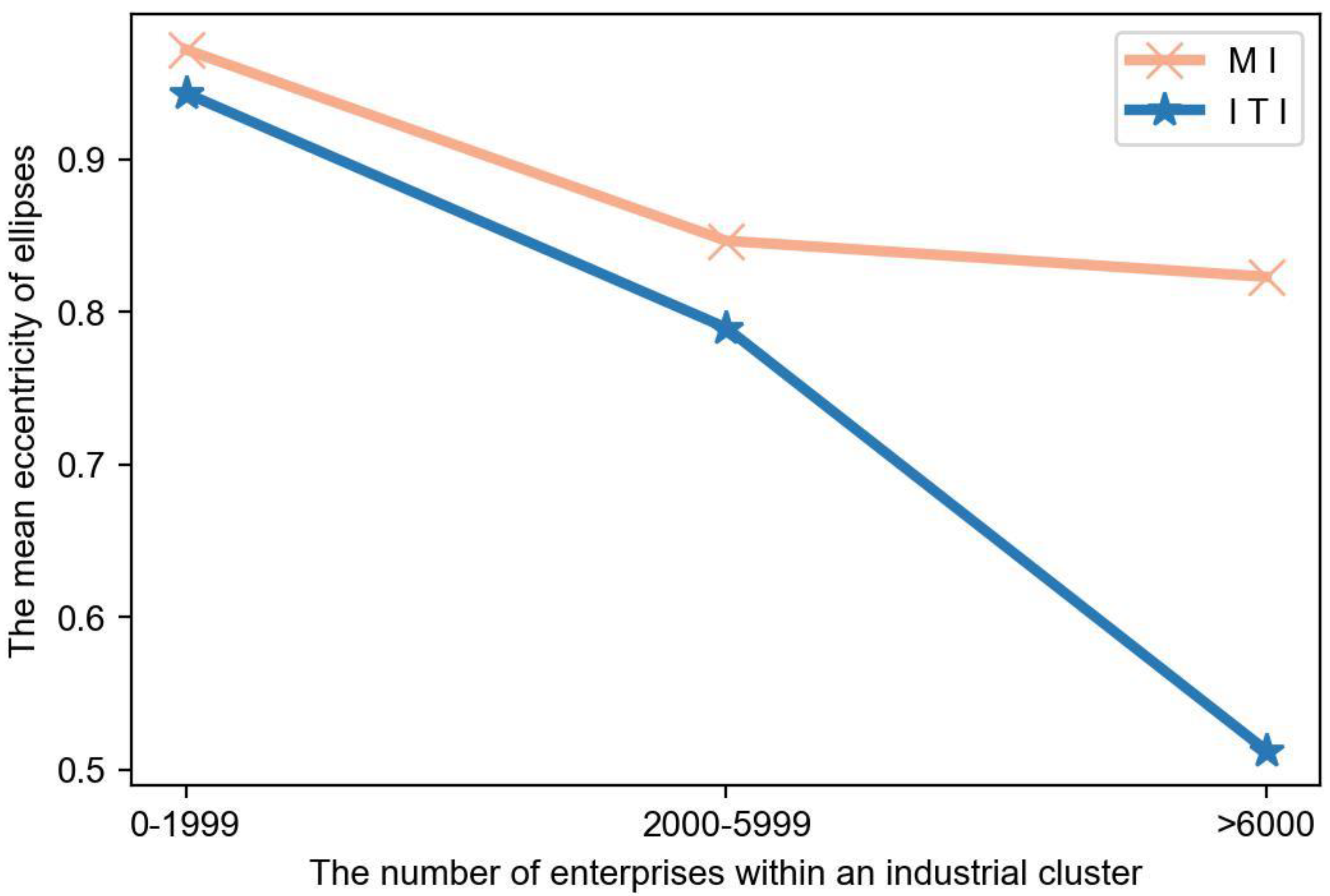
5.1.2. Spatial Form of Industrial Clusters
5.2. Industrial Clusters, Knowledge Spillover and Land Use Efficiency
5.3. Bias in Land Use Efficiency Analysis Based on Administrative Regions
6. Conclusions and Policy Recommendations
Author Contributions
Funding
Data Availability Statement
Conflicts of Interest
References
- Cao, Y.N. Factors affecting on urban location choice decisions of enterprises. Reg. Sci. Inq. 2021, 13, 217–224. [Google Scholar]
- Long, H.; Zhang, Y.; Ma, L.; Tu, S. Land use transitions: Progress, challenges and prospects. Land 2021, 10, 903. [Google Scholar] [CrossRef]
- Ren, X.; Yang, S. Empirical study on location choice of Chinese OFDI. China Econ. Rev. 2020, 61, 101428. [Google Scholar] [CrossRef]
- Gao, X.; Zhang, A.; Sun, Z. How regional economic integration influence on urban land use efficiency? A case study of Wuhan metropolitan area, China. Land Use Policy 2020, 90, 104329. [Google Scholar] [CrossRef]
- Surya, B.; Ahmad, D.N.A.; Sakti, H.H.; Sahban, H. Land use change, spatial interaction, and sustainable development in the metropolitan urban areas, South Sulawesi Province, Indonesia. Land 2020, 9, 95. [Google Scholar] [CrossRef]
- Lai, A.; Yang, Z.; Cui, L. Market segmentation impact on industrial transformation: Evidence for environmental protection in China. J. Clean. Prod. 2021, 297, 126607. [Google Scholar] [CrossRef]
- Ren, S.; Hao, Y.; Wu, H. Government corruption, market segmentation and renewable energy technology innovation: Evidence from China. J. Environ. Manag. 2021, 300, 113686. [Google Scholar] [CrossRef]
- Grossman, G.M.; Helpman, E. Trade, knowledge spillovers, and growth. Eur. Econ. Rev. 1991, 35, 517–526. [Google Scholar] [CrossRef]
- Rosenfeld, S.A. Bringing business clusters into the mainstream of economic development. Eur. Plan. Stud. 1997, 5, 3–23. [Google Scholar] [CrossRef]
- Gottmann, J. Megalopolis or the urbanization of the northeastern seaboard. Econ. Geogr. 1957, 33, 189–200. [Google Scholar] [CrossRef]
- Fei, R.; Lin, Z.; Chunga, J. How land transfer affects agricultural land use efficiency: Evidence from China’s agricultural sector. Land Use Policy 2021, 103, 105300. [Google Scholar] [CrossRef]
- Zhang, W.; Wang, B.; Wang, J.; Wu, Q.; Wei, Y.D. How does industrial agglomeration affect urban land use efficiency? A spatial analysis of Chinese cities. Land Use Policy 2022, 119, 106178. [Google Scholar] [CrossRef]
- Liu, J.; Feng, H.; Wang, K. The low-carbon city pilot policy and urban land use efficiency: A policy assessment from China. Land 2022, 11, 604. [Google Scholar] [CrossRef]
- Li, S.; Fu, M.; Tian, Y.; Xiong, Y.; Wei, C. Relationship between urban land use efficiency and economic development level in the Beijing–Tianjin–Hebei region. Land 2022, 11, 976. [Google Scholar] [CrossRef]
- Alcácer, J.; Zhao, M. Zooming in: A practical manual for identifying geographic clusters. Strateg. Manag. J. 2016, 37, 10–21. [Google Scholar] [CrossRef]
- Duranton, G.; Overman, H.G. Testing for localization using micro-geographic data. Rev. Econ. Stud. 2005, 72, 1077–1106. [Google Scholar] [CrossRef]
- Billings, S.B.; Johnson, E.B. Agglomeration within an urban area. J. Urban Econ. 2016, 91, 13–25. [Google Scholar] [CrossRef]
- Garreton, M.; Basauri, A.; Valenzuela, L. Exploring the correlation between city size and residential segregation: Comparing Chilean cities with spatially unbiased indexes. Environ. Urban. 2020, 32, 569–588. [Google Scholar] [CrossRef]
- Jelinski, D.E.; Wu, J. The modifiable areal unit problem and implications for landscape ecology. Landsc. Ecol. 1996, 11, 129–140. [Google Scholar] [CrossRef]
- Ma, W.; Jiang, G.; Chen, Y.; Qu, Y.; Zhou, T.; Li, W. How feasible is regional integration for reconciling land use conflicts across the urban–rural interface? Evidence from Beijing–Tianjin–Hebei metropolitan region in China. Land Use Policy 2020, 92, 104433. [Google Scholar] [CrossRef]
- Krupka, D.J. Are big cities more segregated? Neighbourhood scale and the measurement of segregation. Urban Stud. 2007, 44, 187–197. [Google Scholar] [CrossRef]
- Xu, B.; Sun, Y. The impact of industrial agglomeration on urban land green use efficiency and its spatio-temporal pattern: Evidence from 283 cities in China. Land 2023, 12, 824. [Google Scholar] [CrossRef]
- Hoover, E.M. Location Theory and the Shoe and Leather Industries; Harvard University Press: Cambridge, MA, USA, 1937. [Google Scholar]
- Weber, A.; Friedrich, C.J. Alfred Weber’s Theory of the Location of Industries; University of Chicago Press: Chicago, IL, USA, 1929. [Google Scholar]
- Marshall, A. Principles of Economics: An Introductory Volume, 8th ed.; Macmillan: London, UK, 1920. [Google Scholar]
- Roelandt, T.J.; den Hertog, P. Cluster analysis and cluster-based policy making: The state of the art. In Boosting Innovation: The Cluster Approach; Organisation for Economic Co-operation and Development (OECD): Paris, France, 1999; pp. 413–427. [Google Scholar]
- Bergman, E.M.; Feser, E.J. Industrial and Regional Clusters: Concepts and Comparative Applications; West Virginal University Press: Morgantown, WV, USA, 1999. [Google Scholar]
- Porter, M.E. Clusters, Innovation, and Competitiveness: New Findings and Implications for Policy. In Proceedings of the European Presidency Conference on Innovation and Clusters, Stockholm, Sweden, 22 January 1998. [Google Scholar]
- Krugman, P. Scale economies, product differentiation, and the pattern of trade. Am. Econ. Rev. 1980, 70, 950–959. [Google Scholar]
- Krugman, P. The increasing returns revolution in trade and geography. Am. Econ. Rev. 2009, 99, 561–571. [Google Scholar] [CrossRef]
- Green, T. Evaluating predictors for brownfield redevelopment. Land Use Policy 2018, 73, 299–319. [Google Scholar] [CrossRef]
- Jamecny, L.; Husar, M. From planning to smart management of historic industrial brownfield regeneration. Procedia Eng. 2016, 161, 2282–2289. [Google Scholar] [CrossRef]
- Martinat, S.; Navratil, J.; Hollander, J.B.; Trojan, J.; Klapka, P.; Klusacek, P.; Kalok, D. Re-reuse of regenerated brownfields: Lessons from an Eastern European post-industrial city. J. Clean. Prod. 2018, 188, 536–545. [Google Scholar] [CrossRef]
- Xie, X.; Wu, K.; Li, Y.; Guo, S.; Li, X. How to Coordinate the Relationship between Urban Space Exploitation, Economic Development, and Ecological Environment: Evidence from Henan Province, China. Land 2024, 13, 537. [Google Scholar] [CrossRef]
- Du, J.; Thill, J.-C.; Peiser, R.B. Land pricing and its impact on land use efficiency in post-land-reform China: A case study of Beijing. Cities 2016, 50, 68–74. [Google Scholar] [CrossRef]
- Louw, E.; van Der Krabben, E.; Van Amsterdam, H. The spatial productivity of industrial land. Reg. Stud. 2012, 46, 137–147. [Google Scholar] [CrossRef]
- Zhang, J.; Zhang, D.; Huang, L.; Wen, H.; Zhao, G.; Zhan, D. Spatial distribution and influential factors of industrial land productivity in China’s rapid urbanization. J. Clean. Prod. 2019, 234, 1287–1295. [Google Scholar] [CrossRef]
- Wey, W.-M.; Hsu, J. New urbanism and smart growth: Toward achieving a smart National Taipei University District. Habitat Int. 2014, 42, 164–174. [Google Scholar] [CrossRef]
- Chen, W.; Shen, Y.; Wang, Y.; Wu, Q. The effect of industrial relocation on industrial land use efficiency in China: A spatial econometrics approach. J. Clean. Prod. 2018, 205, 525–535. [Google Scholar] [CrossRef]
- Ye, L.; Huang, X.; Yang, H.; Chen, Z.; Zhong, T.; Xie, Z. Effects of dual land ownerships and different land lease terms on industrial land use efficiency in Wuxi City, East China. Habitat Int. 2018, 78, 21–28. [Google Scholar] [CrossRef]
- Chen, W.; Chen, W.; Ning, S.; Liu, E.-n.; Zhou, X.; Wang, Y.; Zhao, M. Exploring the industrial land use efficiency of China’s resource-based cities. Cities 2019, 93, 215–223. [Google Scholar] [CrossRef]
- Yu, J.; Zhou, K.; Yang, S. Land use efficiency and influencing factors of urban agglomerations in China. Land Use Policy 2019, 88, 104143. [Google Scholar] [CrossRef]
- Xie, H.; Chen, Q.; Lu, F.; Wang, W.; Yao, G.; Yu, J. Spatial-temporal disparities and influencing factors of total-factor green use efficiency of industrial land in China. J. Clean. Prod. 2019, 207, 1047–1058. [Google Scholar] [CrossRef]
- Shaoa, Y.; Chen, S.; Cheng, B. Analyses of the Dynamic Factors of Cluster Innovation—A Case Study of Chengdu Furniture Industrial Cluster. Int. Manag. Rev. 2008, 4, 53. [Google Scholar]
- Seto, K.C.; Fragkias, M. Quantifying spatiotemporal patterns of urban land-use change in four cities of China with time series landscape metrics. Landsc. Ecol. 2005, 20, 871–888. [Google Scholar] [CrossRef]
- Liu, Y.; Wang, Y.; Wu, L. Review on the definition and mechanism of urban agglomeration and its future research fields. Hum. Geogr. 2013, 28, 62–68. [Google Scholar]
- Yang, Y.; Liu, Y.; Li, Y.; Li, J. Measure of urban-rural transformation in Beijing-Tianjin-Hebei region in the new millennium: Population-land-industry perspective. Land Use Policy 2018, 79, 595–608. [Google Scholar] [CrossRef]
- Meijers, E.J.; Burger, M.J. Spatial structure and productivity in US metropolitan areas. Environ. Plan. A 2010, 42, 1383–1402. [Google Scholar] [CrossRef]
- Zeng, G.; Hu, Y.; Zhong, Y. Industrial agglomeration, spatial structure and economic growth: Evidence from urban cluster in China. Heliyon 2023, 9, e19963. [Google Scholar] [CrossRef]
- Wang, B.; Yang, X.; Dou, Y.; Wu, Q.; Wang, G.; Li, Y.; Zhao, X. Spatio-Temporal Dynamics of Economic Density and Vegetation Cover in the Yellow River Basin: Unraveling Interconnections. Land 2024, 13, 475. [Google Scholar] [CrossRef]
- Lee, J.; Jung, S. Towards Carbon-Neutral Cities: Urban Classification Based on Physical Environment and Carbon Emission Characteristics. Land 2023, 12, 968. [Google Scholar] [CrossRef]
- Brezzi, M.; Veneri, P. Assessing polycentric urban systems in the OECD: Country, regional and metropolitan perspectives. Eur. Plan. Stud. 2015, 23, 1128–1145. [Google Scholar] [CrossRef]
- Kocziszky, G.; Nagy, Z.; Tóth, G.; Dávid, L. New Method for Analysing the Spatial Structure of Europe. Econ. Comput. Econ. Cybern. Stud. Res. 2015, 49, 143–160. [Google Scholar]
- Veneri, P.; Burgalassi, D. Questioning polycentric development and its effects. Issues of definition and measurement for the Italian NUTS-2 regions. Eur. Plan. Stud. 2012, 20, 1017–1037. [Google Scholar] [CrossRef]
- Sun, B.; Li, W. City size distribution and economic performance: Evidence from city-regions in China. Sci. Geogr. Sin. 2016, 36, 328–334. [Google Scholar]
- Liu, X.; Li, S.; Qin, M. Urban spatial structure and regional economic efficiency-on the mode choice of China’s urbanization development. Manag. World 2017, 1, 51–64. [Google Scholar]
- Wang, Z.; Liu, C.; Mao, K. Industry cluster: Spatial density and optimal scale. Ann. Reg. Sci. 2012, 49, 719–731. [Google Scholar] [CrossRef]
- Barbieri, E.; Di Tommaso, M.R.; Bonnini, S. Industrial development policies and performances in Southern China: Beyond the specialised industrial cluster program. China Econ. Rev. 2012, 23, 613–625. [Google Scholar] [CrossRef]
- Belso-Martínez, J.A.; Mas-Verdu, F.; Chinchilla-Mira, L. How do interorganizational networks and firm group structures matter for innovation in clusters: Different networks, different results. J. Small Bus. Manag. 2020, 58, 73–105. [Google Scholar] [CrossRef]
- Hahsler, M.; Piekenbrock, M.; Doran, D. dbscan: Fast density-based clustering with R. J. Stat. Softw. 2019, 91, 1–30. [Google Scholar] [CrossRef]
- Mohring, H. Land values and the measurement of highway benefits. J. Political Econ. 1961, 69, 236–249. [Google Scholar] [CrossRef]
- Morrison, W.M. China’s economic rise: History, trends, challenges, and implications for the United States. Curr. Politics Econ. North. West. Asia 2019, 28, 189–242. [Google Scholar]
- Lian, Z.; Ma, Y.; Chen, L.; He, R. The role of cities in cross-border mergers and acquisitions—Evidence from China. Int. Rev. Econ. Financ. 2024, 92, 1482–1498. [Google Scholar] [CrossRef]
- Wang, S.; Liu, J.; Xu, K.; Ji, M.; Yan, F. Cross-Regional Cooperation and Counter-Market-Oriented Spatial Linkage: A Case Study of Collaborative Industrial Parks in the Yangtze River Delta Region. Int. J. Environ. Res. Public Health 2023, 20, 1055. [Google Scholar] [CrossRef]
- Wang, P.; Zeng, C.; Song, Y.; Guo, L.; Liu, W.; Zhang, W. The spatial effect of administrative division on land-use intensity. Land 2021, 10, 543. [Google Scholar] [CrossRef]
- Wu, L.; Lang, W.; Chen, T. Deciphering Urban Land Use Patterns in the Shenzhen–Dongguan Cross-Boundary Region Based on Multisource Data. Land 2024, 13, 161. [Google Scholar] [CrossRef]
- Zheng, L.; Zhao, Z. What drives spatial clusters of entrepreneurship in China? Evidence from economic census data. China Econ. Rev. 2017, 46, 229–248. [Google Scholar] [CrossRef]
- Yang, S.; Jahanger, A.; Hossain, M.R. How effective has the low-carbon city pilot policy been as an environmental intervention in curbing pollution? Evidence from Chinese industrial enterprises. Energy Econ. 2023, 118, 106523. [Google Scholar] [CrossRef]
- Li, F.; Gui, Z.; Wu, H.; Gong, J.; Wang, Y.; Tian, S.; Zhang, J. Big enterprise registration data imputation: Supporting spatiotemporal analysis of industries in China. Comput. Environ. Urban Syst. 2018, 70, 9–23. [Google Scholar] [CrossRef]
- Fu, X.; Balasubramanyam, V.N. Township and village enterprises in China. J. Dev. Stud. 2003, 39, 27–46. [Google Scholar] [CrossRef]
- Jiang, G.; Ma, W.; Dingyang, Z.; Qinglei, Z.; Ruijuan, Z. Agglomeration or dispersion? Industrial land-use pattern and its impacts in rural areas from China’s township and village enterprises perspective. J. Clean. Prod. 2017, 159, 207–219. [Google Scholar] [CrossRef]
- Walker, R.T. Geography, Von Thünen, and Tobler’s first law: Tracing the evolution of a concept. Geogr. Rev. 2022, 112, 591–607. [Google Scholar] [CrossRef]
- Fischer, K. Central places: The theories of von Thünen, Christaller, and Lösch. In Foundations of Location Analysis; Springer: New York, NY, USA, 2011; pp. 471–505. [Google Scholar]
- Lubis, S.; Siregar, A.M.; Siregar, I. Study of Statically Tested Honeycomb Structure. Int. J. Econ. Technol. Soc. Sci. (Inject.) 2021, 2, 1–12. [Google Scholar] [CrossRef]
- Wang, S.; Feng, Z.; Zhang, S. The Central Place and Diffusion Area System under the View of Economic Region System Theory. Sci. Geogr. Sin. 2010, 30, 803–809. [Google Scholar]
- Ahlfeldt, G.M.; Barr, J. The economics of skyscrapers: A synthesis. J. Urban Econ. 2022, 129, 103419. [Google Scholar] [CrossRef]
- Chen, Y.; Li, S.; Cheng, L. Evaluation of cultivated land use efficiency with environmental constraints in the Dongting lake eco-economic zone of Hunan province, China. Land 2020, 9, 440. [Google Scholar] [CrossRef]
- Zhang, C.; Su, Y.; Yang, G.; Chen, D.; Yang, R. Spatial-temporal characteristics of cultivated land use efficiency in major function-oriented zones: A case study of Zhejiang province, China. Land 2020, 9, 114. [Google Scholar] [CrossRef]
- Liu, S.; Xiao, W.; Li, L.; Ye, Y.; Song, X. Urban land use efficiency and improvement potential in China: A stochastic frontier analysis. Land Use Policy 2020, 99, 105046. [Google Scholar] [CrossRef]
- Ke, X.; Zhang, Y.; Zhou, T. Spatio-temporal characteristics and typical patterns of eco-efficiency of cultivated land use in the Yangtze River Economic Belt, China. J. Geogr. Sci. 2023, 33, 357–372. [Google Scholar] [CrossRef]
- Guo, B.; Chen, K.; Jin, G. Does multi-goal policy affect agricultural land efficiency? A quasi-natural experiment based on the natural resource conservation and intensification pilot scheme. Appl. Geogr. 2023, 161, 103141. [Google Scholar] [CrossRef]
- Liu, X.; Zhang, X. Industrial agglomeration, technological innovation and carbon productivity: Evidence from China. Resour. Conserv. Recycl. 2021, 166, 105330. [Google Scholar] [CrossRef]
- Li, C.; Wu, K.; Gao, X. Manufacturing industry agglomeration and spatial clustering: Evidence from Hebei Province, China. Environ. Dev. Sustain. 2020, 22, 2941–2965. [Google Scholar] [CrossRef]
- Sun, J.; Fan, P.; Wang, K.; Yu, Z. Research on the impact of the industrial cluster effect on the profits of new energy enterprises in China: Based on the Moran’s I index and the fixed-effect panel stochastic frontier model. Sustainability 2022, 14, 14499. [Google Scholar] [CrossRef]
- Ellison, G.; Glaeser, E.L.; Kerr, W.R. What causes industry agglomeration? Evidence from coagglomeration patterns. Am. Econ. Rev. 2010, 100, 1195–1213. [Google Scholar] [CrossRef]
- Zhu, X.; Li, Y.; Zhang, P.; Wei, Y.; Zheng, X.; Xie, L. Temporal–spatial characteristics of urban land use efficiency of China’s 35mega cities based on DEA: Decomposing technology and scale efficiency. Land Use Policy 2019, 88, 104083. [Google Scholar] [CrossRef]
- Koroso, N.H.; Lengoiboni, M.; Zevenbergen, J.A. Urbanization and urban land use efficiency: Evidence from regional and Addis Ababa satellite cities, Ethiopia. Habitat Int. 2021, 117, 102437. [Google Scholar] [CrossRef]
- Reder, M.W. A reconsideration of the marginal productivity theory. J. Political Econ. 1947, 55, 450–458. [Google Scholar] [CrossRef]
- Su, D.; Sheng, B.; Shao, C.; Chen, S. Global value chain, industry agglomeration and firm productivity’s interactive effect. Econ. Res. J. 2020, 55, 100–115. [Google Scholar]
- Zhang, X.; Yao, J.; Sila-Nowicka, K.; Song, C. Geographic concentration of industries in Jiangsu, China: A spatial point pattern analysis using micro-geographic data. Ann. Reg. Sci. 2021, 66, 439–461. [Google Scholar] [CrossRef]
- Zhang, W.; Xu, N.; Li, C.; Cui, X.; Zhang, H.; Chen, W. Impact of digital input on enterprise green productivity: Micro evidence from the Chinese manufacturing industry. J. Clean. Prod. 2023, 414, 137272. [Google Scholar] [CrossRef]
- Jenkins, R.; de Freitas Barbosa, A. Fear for manufacturing? China and the future of industry in Brazil and Latin America. China Q. 2012, 209, 59–81. [Google Scholar] [CrossRef]
- Bao, L.; Li, T.; Xia, X.; Zhu, K.; Li, H.; Yang, X. How does working from home affect developer productivity?—A case study of Baidu during the COVID-19 pandemic. Sci. China Inf. Sci. 2022, 65, 142102. [Google Scholar] [CrossRef]
- Lavoratori, K.; Mariotti, S.; Piscitello, L. The role of geographical and temporary proximity in MNEs’ location and intra-firm co-location choices. Reg. Stud. 2020, 54, 1442–1456. [Google Scholar] [CrossRef]
- Amidi, S.; Majidi, A.F. Geographic proximity, trade and economic growth: A spatial econometrics approach. Ann. GIS 2020, 26, 49–63. [Google Scholar] [CrossRef]
- Löfsten, H.; Isaksson, A.; Rannikko, H. Entrepreneurial networks, geographical proximity, and their relationship to firm growth: A study of 241 small high-tech firms. J. Technol. Transf. 2023, 48, 2280–2306. [Google Scholar] [CrossRef]
- Henderson, J.V. Marshall’s scale economies. J. Urban Econ. 2003, 53, 1–28. [Google Scholar] [CrossRef]
- Moretti, E. The effect of high-tech clusters on the productivity of top inventors. Am. Econ. Rev. 2021, 111, 3328–3375. [Google Scholar] [CrossRef]
- Ellison, G.; Glaeser, E.L. The geographic concentration of industry: Does natural advantage explain agglomeration? Am. Econ. Rev. 1999, 89, 311–316. [Google Scholar] [CrossRef]
- Fan, F.; Lian, H.; Wang, S. Can regional collaborative innovation improve innovation efficiency? An empirical study of Chinese cities. Growth Change 2020, 51, 440–463. [Google Scholar] [CrossRef]
- Shen, N.; Peng, H.; Wang, Q. Spatial dependence, agglomeration externalities and the convergence of carbon productivity. Socio-Econ. Plan. Sci. 2021, 78, 101060. [Google Scholar] [CrossRef]
- Stavroulakis, P.J.; Papadimitriou, S.; Tsioumas, V.; Koliousis, I.G.; Riza, E.; Kontolatou, E.O. Strategic competitiveness in maritime clusters. Case Stud. Transp. Policy 2020, 8, 341–348. [Google Scholar] [CrossRef]
- Zhao, Y.; Liang, C.; Zhang, X. Positive or negative externalities? Exploring the spatial spillover and industrial agglomeration threshold effects of environmental regulation on haze pollution in China. Environ. Dev. Sustain. 2021, 23, 11335–11356. [Google Scholar] [CrossRef]
- Du, J.; Vanino, E. Agglomeration externalities of fast-growth firms. Reg. Stud. 2021, 55, 167–181. [Google Scholar] [CrossRef]
- Xiao, Z.; Yuan, Q.; Sun, Y.; Sun, X. New paradigm of logistics space reorganization: E-commerce, land use, and supply chain management. Transp. Res. Interdiscip. Perspect. 2021, 9, 100300. [Google Scholar] [CrossRef]
- Westerweel, B.; Basten, R.; denBoer, J.; vanHoutum, G.J. Printing spare parts at remote locations: Fulfilling the promise of additive manufacturing. Prod. Oper. Manag. 2021, 30, 1615–1632. [Google Scholar] [CrossRef]
- Wlodarczak, D. Smart growth and urban economic development: Connecting economic development and land-use planning using the example of high-tech firms. Environ. Plan. A 2012, 44, 1255–1269. [Google Scholar] [CrossRef]
- Chen, W.; Huang, X.; Liu, Y.; Luan, X.; Song, Y. The impact of high-tech industry agglomeration on green economy efficiency—Evidence from the Yangtze River economic belt. Sustainability 2019, 11, 5189. [Google Scholar] [CrossRef]
- Sun, Y.; Ma, A.; Su, H.; Su, S.; Chen, F.; Wang, W.; Weng, M. Does the establishment of development zones really improve industrial land use efficiency? Implications for China’s high-quality development policy. Land Use Policy 2020, 90, 104265. [Google Scholar] [CrossRef]
- Qu, X.; Xu, Z.; Yu, J.; Zhu, J. Understanding local government debt in China: A regional competition perspective. Reg. Sci. Urban Econ. 2023, 98, 103859. [Google Scholar] [CrossRef]
- Phelps, N.A.; Fuller, C. Multinationals, intracorporate competition, and regional development. Econ. Geogr. 2000, 76, 224–243. [Google Scholar]


| A | B | C | |||||
|---|---|---|---|---|---|---|---|
| 2 | 4 | 6 | 1 | 3.75 | 3.75 | 4 | 1 |
| 3 | 6 | 3 | 5 | 4 | 3.67 | ||
| 1 | 5 | 4 | 2 | 3.75 | 3.75 | ||
| 5 | 4 | 5 | 4 | ||||
| Mean: 3.75 Variance: 2.60 | Mean: 3.75 Variance: 0 | Mean: 3.17 Variance: 2.11 | |||||
| MI Clusters | ITI Clusters | |
|---|---|---|
| Quantity | 1383 | 571 |
| Mean | 380 | 455 |
| Standard Deviation | 6152 | 4422 |
| Minimum Value | 10 | 10 |
| Maximum Value | 219,697 | 95,303 |
| MI | ITI | ||||
|---|---|---|---|---|---|
| Quantity | Percentage | Quantity | Percentage | ||
| provincial boundaries | type I | 45 | 3.3% | 33 | 5.8% |
| type II | 0 | 0.0% | 0 | 0.0% | |
| type III | 1338 | 96.7% | 538 | 94.2% | |
| city boundaries | type I | 173 | 12.5% | 112 | 19.6% |
| type II | 1 | 0.1% | 0 | 0.0% | |
| type III | 1209 | 87.4% | 459 | 80.4% | |
| MI | ITI | |
|---|---|---|
| Moran’s I | −0.002 * | −0.016 *** |
| Z statistic | −1.819 | −6.319 |
| MI | ITI | |||
|---|---|---|---|---|
| SEM | SAR | SEM | SAR | |
| Scale of industrial clusters | 0.0200 *** (7.3182) | 0.0200 *** (7.2825) | 0.0432 *** (6.6154) | 0.0433 *** (6.5883) |
| Spatial lag parameter | 0.2869 (0.7604) | 0.1140 (0.2758) | ||
| Spatial error parameter | 0.3801 (1.1008) | 0.2014 (0.5015) | ||
| Constant | 0.0286 *** (3.0786) | 0.0017 (0.479) | 0.0312 (1.5725) | −0.0123 (−0.1811) |
| 0.0366 | 0.0365 | 0.0707 | 0.0708 | |
| Observations | 1383 | 1383 | 571 | 571 |
| MI | ITI | |||
|---|---|---|---|---|
| DEA-SBM | DEA-EBM | DEA-SBM | DEA-EBM | |
| Scale of industrial clusters | 0.0350 *** | 0.0308 *** | 0.0524 *** | 0.0562 *** |
| (14.0934) | (11.4187) | (15.1020) | (15.4485) | |
| Spatial error parameter | −1.0 * | −1.0 * | −0.0846 | −0.05327 |
| (−1.7822) | (−1.7822) | (−0.1821) | (−0.116) | |
| Constant | −0.0806 *** | −0.0067 | −0.1826 *** | −0.1634 *** |
| (−4.3408) | (−0.3335) | (−7.7319) | (−6.5898) | |
| 0.1226 | 0.0833 | 0.2866 | 0.2955 | |
| Observations | 1383 | 1383 | 571 | 571 |
| SEM | OLS | ||
|---|---|---|---|
| MI | Scale of industrial clusters | 0.0166 *** | 0.0197 *** |
| (7.2467) | (7.209) | ||
| Spatial error parameter | 0.2857 | ||
| (0.7523) | |||
| Constant | 0.0003 | 0.0283 *** | |
| (−0.0197) | (3.152) | ||
| 0.0363 | 0.0360 | ||
| Observations | 1383 | 1383 | |
| ITI | Scale of industrial clusters | 0.0411 *** | 0.0426 *** |
| (11.0239) | (6.521) | ||
| Spatial error parameter | 0.1225 | ||
| (0.2901) | |||
| Constant | −0.0504 *** | 0.0311 | |
| (−2.5925) | (1.599) | ||
| 0.1753 | 0.0690 | ||
| Observations | 571 | 571 | |
| MI | ITI | |
|---|---|---|
| LM spatial lag | 0.9539 | 14.985 *** |
| LM spatial error | 0.0075 | 17.7269 *** |
| Robust LM spatial lag | 3.1896 * | 1.806 |
| Robust LM spatial error | 2.2433 | 4.5479 ** |
| Wald test spatial error | 2.1098 | 0.6051 |
| LR test spatial error | −38221.6852 | −1048.1255 |
Disclaimer/Publisher’s Note: The statements, opinions and data contained in all publications are solely those of the individual author(s) and contributor(s) and not of MDPI and/or the editor(s). MDPI and/or the editor(s) disclaim responsibility for any injury to people or property resulting from any ideas, methods, instructions or products referred to in the content. |
© 2024 by the authors. Licensee MDPI, Basel, Switzerland. This article is an open access article distributed under the terms and conditions of the Creative Commons Attribution (CC BY) license (https://creativecommons.org/licenses/by/4.0/).
Share and Cite
Cui, Y.; Niu, Y.; Ren, Y.; Zhang, S.; Zhao, L. A Model to Analyze Industrial Clusters to Measure Land Use Efficiency in China. Land 2024, 13, 1070. https://doi.org/10.3390/land13071070
Cui Y, Niu Y, Ren Y, Zhang S, Zhao L. A Model to Analyze Industrial Clusters to Measure Land Use Efficiency in China. Land. 2024; 13(7):1070. https://doi.org/10.3390/land13071070
Chicago/Turabian StyleCui, Yanzhe, Yingnan Niu, Yawen Ren, Shiyi Zhang, and Lindan Zhao. 2024. "A Model to Analyze Industrial Clusters to Measure Land Use Efficiency in China" Land 13, no. 7: 1070. https://doi.org/10.3390/land13071070