Interaction Effect of Carbon Emission and Ecological Risk in the Yangtze River Economic Belt: New Insights into Multi-Simulation Scenarios

Abstract

The scientific quantification of the ecological effects of carbon emissions, the reduction of ecological risk (ER), and the evaluation of the interaction effect between carbon emissions and ER are the pivotal measures for ensuring the longevity and continuity of sustainability. However, a dearth of comprehensive and macro-level evaluations exist pertaining to the ER and carbon emissions within the entirety of the Yangtze River Economic Belt (YREB). We have constructed four distinct simulated scenarios within the YREB, which include natural development (ND), cultivated land protection (CLP), ecological conservation (EC), and low carbon (LC) scenarios. Based on the consideration of future uncertainty, we predicted LUCEs and ERI under different scenarios, and analyzed the spatial interaction effects of LUCEs and ERI from the dual perspectives of the spatial spillover effect and spatial coupling effect. The results showed that under the four outlined scenarios, encompassing diverse parameters, conversion possibilities, and areas subject to restrictions, the land utilization patterns of the YREB in 2030 have unveiled pronounced disparities. The LUCEs in the YREB showed significant spatial heterogeneity under the four scenarios; the maximum value was 6.65 under the CLP scenario and the minimum value was 4.65 under the LC scenario. The ER has the highest value under the ND scenario and the lowest value under LC scenario. Construction land is the largest contributor to increased LUCEs, and forest land is the form of terrestrial utilization that reduces the impact of LUCEs. In different scenarios, LUCEs have a significant negative spillover effect on ER, while the bidirectional spatial coupling effect between LUCEs and ERI presents significant differences. Under the LC scenario, land with a strong carbon sequestration capacity increased significantly, the fragmentation of water bodies was alleviated, and the CCD was the highest. This study offers scientific counsel for the sustainable development of various regions within the YREB, thereby fostering the achievement of a harmonious coexistence between the ecological milieu and economic development.

1. Introduction

The Sustainable Development Goals (SDGs) aspire to propel the global community towards a sustainable developmental trajectory by holistically addressing the social, economic, and environmental development facets in a cohesive fashion from 2015 to 2030 [1]. SDG11 endeavors to foster the creation of encompassing, safe, resilient, and continuable urban habitats for people, at a juncture when swift economic advancement has intensified the discord between humanity and its terrestrial environments, augmented the threshold of the ecological milieu, and engendered inevitable perils for ecosystems [2]. The issue of global warming has emerged as the preeminent environmental concern on a global scale. Within this framework, there has been a confluence of international agreement that aimed at diminishing carbon emissions. Notably, the augmentation of atmospheric carbon dioxide concentration stemming from alterations in land use constitutes the predominant contributor to total carbon emissions [3]. It is of paramount importance to delve into the mitigation of carbon emissions through the lens of land use. Such exploration will enable the discovery of a novel equilibrium between the swift pace of urbanization and the preservation and enhancement of the ecological milieu, ultimately fostering a harmonious and sustainable synergy between the two [4]. SDG15 centers its attention on the safeguarding, rejuvenation, and advancement of the sustainable utilization of terrestrial ecosystems, alongside the prudent utilization and governance of land resources [5]. The terrestrial landscape assumes a paramount role as the primary conduit for carbon exchange in both human endeavors and the broader terrestrial ecosystem. Hence, considering the novel paradigm of land resources, it holds paramount practical significance to enhance and safeguard the ecosystem while concurrently mitigating the ecological risk (ER). Thus, the prognostication of forthcoming land use and coverage alterations via multi-faceted scenario simulations, along with the projection of carbon emissions and the evolutionary trajectory of ER, can furnish a scientific cornerstone for prospective land use governance decisions. This holds profound implications for shaping strategies aimed at curtailing carbon emissions and advocating for the preservation and revitalization of ecosystems.

As science and technology advance and the global population burgeons, the influence of human endeavors on the natural world has escalated in both magnitude and scope; this has engendered a plethora of predicaments [6], such as ecological function deterioration and landscape pattern disintegration [7]. ER refers to the possibility and loss of uncertain accidents and human activities in a certain region that exert detrimental influences on the framework and functionality of the ecosystem, thereby precipitating a precarious situation concerning the welfare and ecological balance of the habitat [8]. The ecosystem exhibits great diversity and intricacy; the intricate nature of ER has led to a proliferation of diverse risk sources, with risk factors transcending singular scales [2,9]. The methodologies for ER assessments have evolved from subjective qualitative evaluations to objective quantitative analyses [10]. In the domain of quantitative assessment, potential ecosystem risks are quantified and predicted through the use of mathematical models and statistical analysis [11]. However, it oftentimes overlooks the evaluation of potential implications for human welfare [12]. Moreover, the majority of existing approaches for quantifying ecological risks are static models, limiting their capacity to appraise the spatio-temporal dynamics of ecological risks from a future stance [13]. Hence, the comprehensive consideration of prospective scenarios of uncertainty and their integration into the evaluative framework can engender illumination regarding land utilization prospects and evaluations of climatic and socio-economic determinants. Statistics indicate that the majority of developed nations globally have reached their carbon peak, with carbon emissions exhibiting a discernible downward trajectory [14]. Whilst the carbon emissions of China have undergone a deceleration in recent years, they continue to demonstrate an upward trajectory, with the carbon peak objective remaining unattained [15]. As the product of socio-economic advancement, carbon emissions constitute a significant catalyst for the greenhouse effect, particularly in relation to alterations in land utilization [16]. Thus, unveiling the spatio-temporal dimensions of carbon emissions based on land use changes, and identifying targeted strategies for emission reductions, will serve as a guiding framework for land utilization and enhancements in societal economic welfare [17]. And with the proposed “two-carbon” target, the prediction of future carbon impact has become the focus of research. Therefore, in this study, coupling the PLUS model with the gray forecast model to forecast land use carbon emissions (LUCEs) not only fills the gap of energy consumption prediction in existing studies, but also makes up for the deficiency of carbon emission forecasts, considering future uncertainties.

At present, the commonly used land use pattern prediction methods mainly include the Markov model, cellular automata (CA) model, multi-agent (MAS) model, land use change and effects (CLUE-S) model, future land use prediction (FLUS) model, and patch generation land use change simulation (PLUS) model. Existing studies have shown that the Markov model has good practicability in predicting land use quantity change [18], but it is difficult to reflect the change characteristics of spatial patterns. Many existing CA models are unable to analyze the mechanism of land use change in a specific time period in the simulation process, nor can they simulate the patch evolution of multiple land use types on a spatio-temporal scale [19], especially the patch evolution of natural land use types (forest, grassland, etc.), which limits the application of CA models in actual planning or policy making. The CLUE-S model, as a spatial simulation model, is mainly used to analyze the spatial distribution characteristics of land use change [20], but there are some shortcomings in the prediction of future land quantity. The PLUS model was published and promoted by Liang et al. [21] in 2020. Different from previous CA models, the operational complexity of the PLUS model does not increase exponentially with the increase in land conversion types, and it can also simulate the spatio-temporal dynamics of patches of various land use types, and the model is built based on historical “change” analysis. Land use conversion rules for specific time intervals are available. Therefore, the model has many advantages in terms of applicability, flexibility, and simulation ability, and has been widely used and referenced by many scholars in a short time. The PLUS model coupled a land expansion analysis strategy, LEAS rules mining framework, and a CA model based on multi-type random patch seeds (CARS). The rule mining framework of LEAS is mainly used to superimpose two phases of land use data, extract the expansion area of each land use type, and then calculate the development probability of each land use type and the contribution of each impact factor to the expansion of each land use type through the random forest algorithm. CARS mainly used the multi-type random patch seed mechanism based on threshold decline to dynamically simulate the automatic patch generation process under the restriction of the development probability of each land use type. To sum up, on the one hand, the PLUS model can better analyze the internal factors affecting land use change; on the other hand, the CA model based on multi-type random patch seeds combines the mechanism of random seed generation and threshold decline, and has advantages in simulating spatio-temporal dynamic changes of land use at a regional scale. In addition, the YREB is selected as the research area in this study, and the PLUS model is very suitable for the research scale of this study.

In the context of climate warming and increasingly prominent ecological environmental problems, with rapid economic development and changing land use patterns, ecosystems are affected to varying degrees [22]. It is particularly important to concentrate on the quantitative research of the interaction effect between LUCEs and ER. The interplay between ER and LUCEs entails a complex mechanism characterized by interdependence and mutual restriction [23]. The harmonized progress of these two elements holds great significance in achieving regional sustainable development. Nevertheless, an inadequacy of pertinent investigations exists concerning the interaction effect between LUCEs and ER. What is more, as land use modes and patterns undergo continuous changes, their dynamic impact on the ecological environment becomes apparent. However, prevailing studies primarily employ static indicators of the study area to conduct quantitative pattern optimization analysis, neglecting to establish dynamic spatial pattern simulations for land use analysis. Thus, in this study, the spatial panel model, which is based on spatial econometrics, is used for the first time to take into account the details of the spatial effects of LUCEs and comprehensively consider the spatio-temporal heterogeneity of ER, so as to further quantify the spatial spillover effects of LUCEs on ER more accurately. After this, the coupling coordination degree model is further introduced, which can more comprehensively consider the spatial interaction between LUCEs and ER, identify potential risks and vulnerabilities between systems, and thus more comprehensively evaluate the overall stability of the system.

The Yangtze River Economic Belt (YREB) is a leading demonstration belt for the construction of an inland economic belt and is an ecological civilization with global influence, which occupies a pivotal position in China’s regional development landscape. Therefore, taking the YREB as an example, this study attempts to (1) examine the spatial attributes of LUCE and ER analyses, while taking into account future uncertainty scenarios, and (2) systematically evaluate the dynamic interaction response between LUCEs and ER in terms of the spatial spillover effect and bidirectional coupling effect.

2. Material and Methods

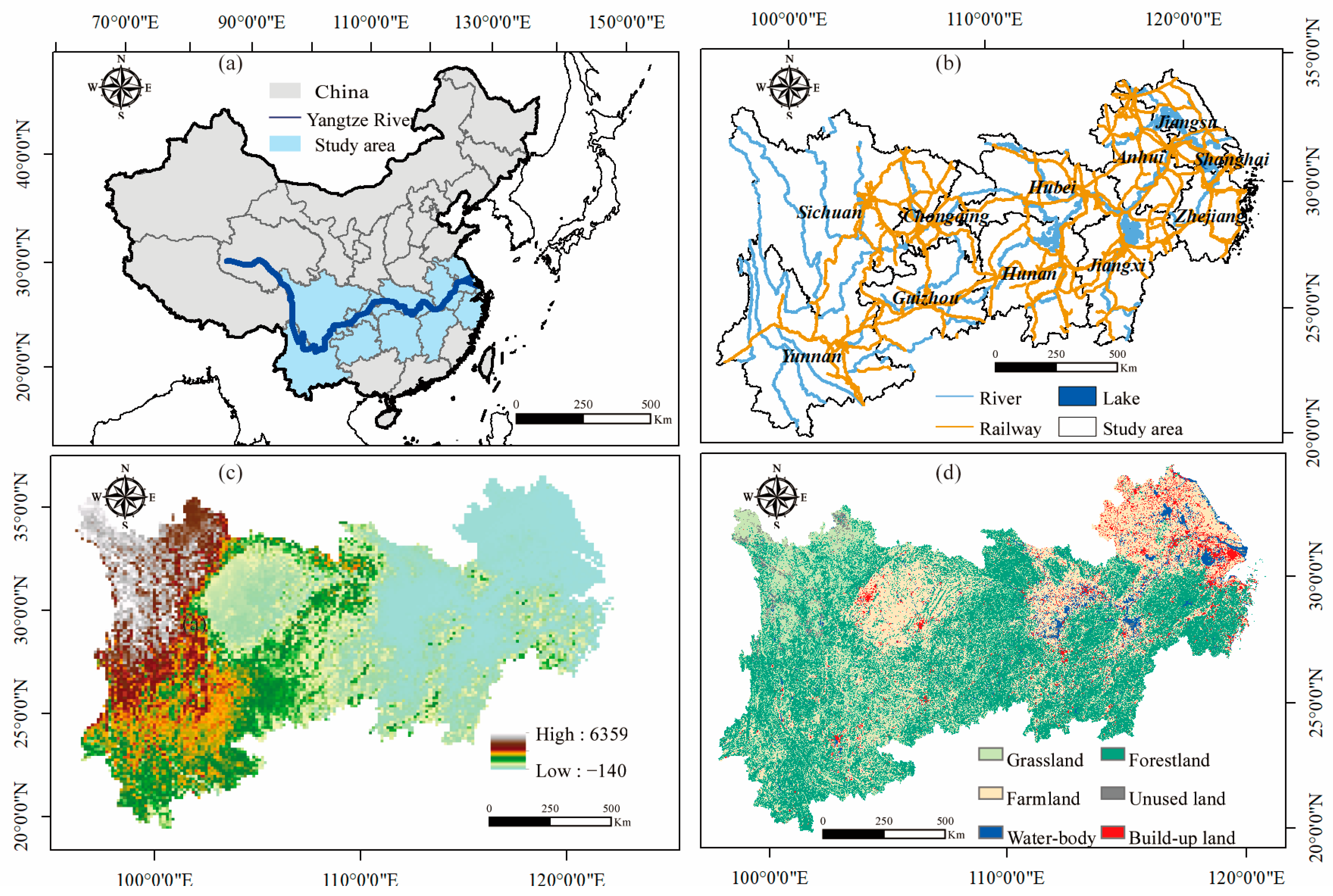
2.1. Study Area

In 2020, the YREB’s permanent population surpassed 43.00% of the national total, with the local economic productivity contributing to 46.40% of the national total. Moreover, the YREB exhibits a complex and diverse geographical landscape. It encompasses various types of ecological environments and environmental issues, as well as a complete basin ecosystem. The region has abundant water resources, boasting an impressive storage capacity surpassing 961.6 billion cubic meters. Additionally, its total grain yield, reaching approximately 238 million tons in the year 2020, signifies a notable 35.85% contribution to the national aggregate. Additionally, the region serves as a significant ecological treasury in China, boasting a forest coverage rate of 41.3%. Promoting the development and construction of the YREB is a crucial national strategy for our country, placing regional green development and ecological sustainability in a position of priority to drive high-quality development in a coordinated, balanced, and innovation-driven manner (Figure 1).

2.2. Data Sources

The main data include land utilization data, accessed from the Chinese Academy of Sciences Data Center (https://www.resdc.cn/, accessed on 21 June 2024), with a spatial resolution of 1 km. Digital elevation data (DEM) were accessed from the Geospatial Data Cloud Platform (http://www.gscloud.cn, accessed on 21 June 2024), and slope data with a resolution of 30 m. The influencing factors, including population, GDP, soil type, annual mean temperature, and annual precipitation spatial distribution data with a resolution of 1 km, are from the Resources and Environmental Science and Technology Data Center (http://www.resdc.cn/, accessed on 21 June 2024). Location data of primary, secondary, and tertiary roads and government residences are derived from the BIGMAP map downloader (http://www.bigemap.com, accessed on 21 June 2024). The river system data are from the Scientific Data Center (https://data.tpdc.ac.cn, accessed on 21 June 2024). Grain output, planting area, and energy consumption come from the Statistical Yearbook (2021) and the China Agricultural Product Price Survey Yearbook for 2021. Finally, the spatial resolution of all data is unified to 1 km.

2.3. Methods

Through the integration of pertinent data, encompassing land resources and socio-economic data, and mindful of inherent uncertainties, this study quantifies the ER and LUCEs of the YREB based on multi-simulation scenarios. Furthermore, the spatial interaction response mechanism of LUCEs and ER is described more comprehensively and quantitatively from the two aspects of the spatial spillover effect and bidirectional coupling effect (Figure 2).

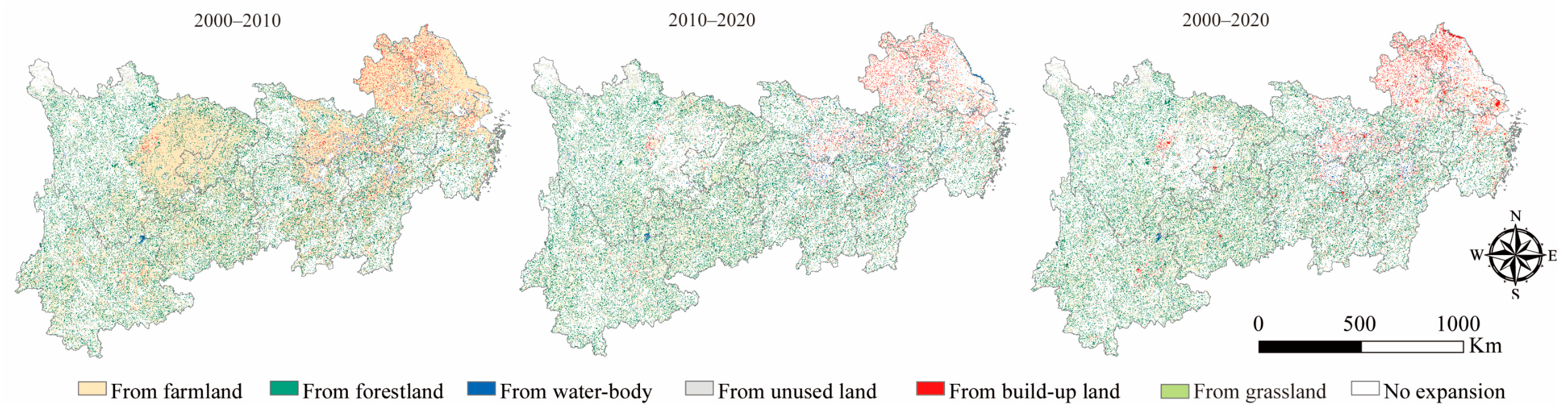
2.3.1. Geoinformation Tupu Method

Rooted in the amalgamation of GIS and graph theory, the Geoinformation Tupu method elucidates interrelationships, configurations, and trajectories within geographic data. This cartographic approach enables a holistic understanding of geographical phenomena and their spatial interconnectedness by translating geographic data into the vertices and edges of a graph, thus capturing the intricate relationships among these vertices [24]. The Geoinformation Tupu method is a spatio-temporal composite analysis method with the ultimate goal of realizing regional sustainable development, which can dynamically visualize multidimensional spatio-temporal information about land use change in the form of atlas units, and has the compound characteristics of quantitatively expressing “spatial patterns” and “temporal characteristics” under multi-spatio-temporal conditions [25]. Considering and subdividing the spatial transfer and change in various land use types at the same time, compared with traditional statistical analysis and static expression methods, it can make up for the change in the geographical location of non-spatial attribute data, and can depict the spatio-temporal dynamic evolution process of various types of land use more accurately and precisely, which has obvious advantages in analyzing land use data [26]. The information atlas of land use change has a good indication of the spatial location and spatial behavior of land use change, and makes the process of land use change linear and dynamic, which is conducive to giving full play to the advantages of the atlas model in data mining and knowledge discovery, and further deepens the mining and multidimensional expression of the inherent laws of land use change [27]. This study chooses the YREB mega-urban agglomeration as the research object, and the research scale is grid-like, which breaks the barriers between administrative units, and can further carry out data mining and analysis. The formulation was defined as follows [28]:

$$G=G_1\times {10}^{\left(n-1\right)}+G_2\times {10}^{\left(n-2\right)}+G_n\times {10}^{\left(n-n\right)}$$

(1)

where $\mathrm{G}$ stands for synthetic land use coding, n represents the number of study periods, and ${\mathrm{G}}_{\mathrm{n}}$ refers to the land utilization category at time t.

2.3.2. Land Use Simulation

1. PLUS model

The PLUS model serves as a sophisticated forecast model for predicting land use change within specific patches [21]. On account of the land utilization from the years 2000 and 2010 of the YREB, coupled with a comprehensive review of the existing literature pertaining to this specific study area, this investigation selected nine driving factors, encompassing both the natural and the economic realms. Then, the analysis of evolving probabilities for each land use type was undertaken employing the LEAS module. The resulting simulation boasted a Kappa coefficient of 0.87 and overall precision of 94.2%, thus underscoring the efficacy of the PLUS model for the precise prediction of future land patterns of the YREB. Consequently, building upon the land usage data from 2020, this study proceeds with a projection of the land utilization pattern anticipated in the YREB for the year 2030.

2. Scenario-setting and parameters

The future transition in land utilization will be profoundly influenced by the accessibility of regional resources, regional economic prowess, and diverse development strategies. Thus, combined with the actual situation in the YREB and the guidance of national policies, and taking into account historical changes and future development trends, this study sets up the following four development scenarios. Therefore, the numerical calculation of scenario-setting in this study is based on considering the regional development level of the Yangtze River Economic Belt (YREB) and referring to the relevant literature [22].

(1) The natural development (ND) scenario

The ND scenario is constructed upon the dynamic fluctuation of land utilization in the YREB spanning from 1990 to 2020, encompassing the innate evolution of diverse land utilization types and the extent of interchanges amongst different regions. While disregarding the sway and constraints imposed by policy planning, the predictive prowess of Markov modeling is harnessed to estimate the scale parameters corresponding to each land utilization category for the year 2030, as detailed in the previous research. It is essential to underline that the ND scenario provides the foundation upon which all other distinctive scenarios are established.

(2) The cultivated land protection (CLP) scenario

The preservation of farmland constitutes a vital foundation for ensuring the sustenance of a nation’s overall food security. As per the Framework for Ensuring Ecological Preservation and Facilitating Exemplary Development within the YREB, China shall persist in fortifying its stature as a prominent grain-producing powerhouse by the year 2030. The farmland preservation scenario comprehensively addresses the imperative of safeguarding agricultural land within the urban agglomeration of the economic belt. Hence, it is imperative to diminish the probability of arable land to accommodate urbanization, afforestation efforts, and the expansion of water bodies by a notable reduction of 40%, 20%, and 20%, respectively [29].

(3) The ecological conservation (EC) scenario

At present, the biggest problem in the development of the YREB is the ecological fragility. The scenario seeks to align with the imperatives of ecological preservation and the pursuit of superior growth within the YREB, and promote harmony between people and land. Based on the ND scenario, the water body is set as a restricted conversion zone. The probability of grassland transitioning into unused land decreased by 40%, while the reduction in transfer probability was even more accentuated for forestland. Within the context of the YREB, forestland stands as a paramount ecological entity. In this regard, the transfer probability of forestland towards developed areas underwent a decline of 40%, while a more modest reduction of 20% was observed for its transition towards unused land. It is essential to note that farmland serves crucial ecological functions, thus necessitating a prudent approach. Consequently, the transfer probability of farmland towards unutilized land declined by 30% [30].

(4) The low carbon (LC) scenario

The LC scenario is a carbon peaking target-oriented plan that scientifically carries out carbon source spatial management and carbon sink spatial protection, adhering to the concept of systematic development in accordance with the Action Plan for Carbon Peaking before 2030; the transfer ratio of forestland, water bodies, and grassland to built-up land should be reduced by 45%, 40%, and 20%, respectively, and the reduced area should be increased to forestland, water bodies, and grassland, respectively, and the water bodies of the YREB should be regarded as a restricted area [31].

3. Conversion rules

The conversion rules encompass both a conversion matrix and the weighting of neighboring factors. The capacity to transform one land use category into another is contingent upon the values ascribed within the conversion matrix. A value of 0 denotes an impossibility for conversion, while a value of 1 signifies the feasibility of the conversion. The establishment of the cost matrix in various scenarios is exemplified in the following

Table 1. Conversion cost matrix for each scenario.

2020–2030	ND Scenario						CLP Scenario						EC Scenario						LC Scenario
	a	b	c	d	e	f	a	b	c	d	e	f	a	b	c	d	e	f	a	b	c	d	e	f
a	1	1	1	1	1	1	1	0	0	0	0	0	1	1	1	1	1	1	1	1	1	1	1	1
b	1	1	1	1	1	1	1	1	1	1	1	1	0	1	0	0	0	0	0	1	0	0	0	0
c	1	1	1	1	1	1	1	1	1	1	1	1	1	1	1	1	1	1	0	1	1	1	0	0
d	1	1	1	1	1	1	1	1	1	1	1	1	0	0	0	1	0	0	0	1	0	1	0	0
e	0	0	0	0	1	0	0	0	0	0	1	0	0	0	0	0	1	0	0	0	0	0	1	0
f	1	1	1	1	1	1	1	1	1	1	1	1	1	1	1	1	1	1	0	1	1	1	0	1

Note: a, b, c, d, e, f respectively, stand for farmland, forestland, grassland, water body, built-up land, and unused land. 0 denotes the prohibition of conversion, while 1 signifies the permission to convert. The rows in the matrix represent roll-outs and the columns represent roll-ins. ND is for natural development, CLP is for cultivated land protection, EC is for ecological conservation, and LC is for low carbon.

.

The precise neighborhood weights assigned to different land use types across the various scenarios are indicated in the subsequent tabular representation (

Table 2. Land use neighborhood weights for each scenario.

Scenarios	Neighborhood Weights
	Farmland	Forestland	Grassland	Water Body	Built-Up Land	Unused Land
ND scenario	0.20	0.30	0.30	0.40	1.00	0.25
CLP scenario	0.80	0.30	0.30	0.40	0.80	0.25
EC scenario	0.20	0.75	0.40	0.75	0.80	0.25
LC scenario	0.20	0.80	0.50	0.75	0.75	0.25

Notes: ND is for natural development, CLP is for cultivated land protection, EC is for ecological conservation, and LC is for low carbon.

).

4. Model accuracy verification

In order to ascertain the precision of the PLUS model, we juxtaposed its simulated outcomes with the actual land utilization patterns observed in the YREB region in the year 2020. The foundation of this investigation rested upon the utilization of the Figure of Merit (FoM) coefficient, a discerning parameter employed to evaluate the veracity of the simulation outcomes. This scrutinization affirms the dependability and practicality of the PLUS model [32].

$$FoM=\frac{B}{A+B+C+D}$$

(2)

In this context, let us consider the variables A, B, C, and D, each symbolizing distinct conditions pertaining to pixel modifications. A denotes the count of pixels erroneously projected as changed, while B is the count of pixels correctly predicted as changed. Additionally, C is the count of pixels inaccurately predicted to change, yet remaining unchanged. D denotes the quantity of pixels that were initially anticipated to remain unaltered but, in reality, experienced alterations [31].

2.3.3. Gray Forecast Model

The gray prediction model is mainly used to effectively predict the time series of small sample data. It uses differential equations to fully excavate the nature of data, requires less information for modeling, has higher prediction accuracy, is more accurate than the traditional time series analysis method, is convenient for statistical testing, and has strong robustness [33]. The gray forecast model is suitable for exponential growth forecasting, such as water consumption forecasting and industrial output value forecasting. Taking the total energy consumption of the YREB, this paper forecasted and tested the energy consumption in 2030 based on the energy consumption from 2000 to 2020, and which is a first-order cumulative generation of the original data series; a first-order linear differential equation model is established, and a fitting curve is obtained, so as to predict the system. The process is as follows: ${\mathrm{x}}^{\left(0\right)}$ is set as the original data, and ${\mathrm{x}}^{\left(0\right)}$ is accumulated once to generate a generation ${\mathrm{x}}^{\left(1\right)}$. Thus, the differential equation of the whitening form can be established:

$$\frac{d{X}^{\left(1\right)}}{dt}+a{X}^{\left(1\right)}=u$$

(3)

The parameters $\mathsf{\alpha }$ and $\mathrm{u}$ are determined through the implementation of the least square method:

$$\left[\begin{array}{c}\alpha \\ u\end{array}\right]=\left(B^{T}B\right)-1B^T{Y}^M$$

(4)

$$\mathrm{B}=\left|\begin{array}{cc}-\frac{1}{2}(x^{\left(1\right)}\left(1\right)+x^{\left(1\right)}\left(2\right))& 1\\ -\frac{1}{2}(x^{\left(1\right)}\left(2\right)+x^{\left(1\right)}\left(3\right))& 1\\ ⋮& ⋮\\ -\frac{1}{2}(x^{\left(1\right)}\left(n-1\right)+x^{\left(1\right)}\left(n\right))& 1\end{array}\right|$$

(5)

$$Y_M={\left[\begin{array}{c}{x}^{\left(0\right)}\left(2\right)\\ x^{\left(0\right)}\left(3\right)\\ ⋮\\ x^{\left(0\right)}\left(n\right)\end{array}\right]}^T$$

(6)

The time response function corresponding to the differential equation, that is, the basic formula of the series prediction, is as follows:

$$x^{\left(1\right)}\left(k+1\right)=\left[x^{\left(0\right)}\left(1\right)-\frac{u}{\alpha }\right]e^{-ak}+\frac{u}{\alpha }$$

(7)

The posterior difference ratio (C) and average relative error ($\overline{\mathsf{\epsilon }}$) were defined as follows:

$$\mathrm{C}=\frac{S_2}{S_1}$$

(8)

$$\overline{\epsilon }=\frac{\sum _{i=1}^n{\epsilon }_i}{n}=\frac{{\sum }_{i=1}^n(\left|residual\right|/Originalvalue)}{n}$$

(9)

where S₁ is the standard deviation of the original data; S₂ is the standard deviation of predicted data; $\mathsf{\epsilon }$ is predicted data error; $\overline{\mathsf{\epsilon }}$ is the mean value of prediction error; and n indicates the year. The C value serves as an indicator of the dispersion magnitude with the forecasted and real values. A smaller C value signifies greater precision, signifying a more discrete original dataset, and a lower degree of discreteness in prediction errors, ultimately leading to heightened prediction accuracy. In the instance where the C value of the posterior variance ratio falls below 0.35, it can be deduced that the model accuracy is commendable. Similarly, if the C value is less than 0.5, the model accuracy is deemed satisfactory. When the C value is lower than 0.65, the evaluation of the model accuracy is essentially acceptable. Conversely, if the C value exceeds 0.65, the model accuracy is deemed inadequate. Notably, a lower average error, denoted as $\overline{\mathsf{\epsilon }}$, signifies a higher level of precision in fitting.

2.3.4. Land Use Carbon Emission (LUCE) Model

The assessment of LUCEs encompasses both direct and indirect assessments. Direct carbon emissions arise primarily from land use transformations. Notably, cultivated land, forestland, grassland, unused land, and water bodies can be regarded as direct sources of carbon emissions. Conversely, indirect carbon emissions within the domain of land use materialize through human activities, specifically within constructed land areas, thereby constituting indirect sources of carbon emissions.

1. Direct carbon emission calculation

Direct carbon emissions were calculated as follows:

$$E_k=\sum e_i=\sum T_i{\delta }_i$$

(10)

where ${\mathrm{E}}_{\mathrm{k}}$ is the total direct carbon emission (t); ${\mathrm{e}}_{\mathrm{i}}$ refers to the carbon emissions corresponding to diverse land utilization categories (t); ${\mathrm{T}}_{\mathrm{i}}$ refers to the acreage of the i species (hm²); and ${\mathsf{\delta }}_{\mathrm{i}}$ is the carbon emission coefficient (t/t) of the i species.

2. Indirect carbon emissions calculation

The direct quantification of carbon emissions originating from land development cannot be ascertained solely based on land area data. This investigation employs an indirect approach to estimate the carbon emissions associated with urban expansion, considering the carbon emissions resulting from both production and daily activities within built-up areas. The carbon emission calculations pertaining to built-up land is as follows:

$$E_x=\sum e_j=\sum M_j·n_j·{\epsilon }_j$$

(11)

where ${\mathrm{E}}_{\mathrm{x}}$ is the cumulative carbon emissions from the designated land over a given time period (t). Meanwhile, the variable ${\mathrm{e}}_{\mathrm{j}}$ denotes the carbon emissions associated with the j-th energy source, among the eight specified energy sources. Furthermore, ${\mathrm{M}}_{\mathrm{j}}$ signifies the annual utilization of the j-th energy source in tons (t), while ${\mathrm{n}}_{\mathrm{j}}$ represents the conversion coefficient for standard coal per ton (kgce/t) or per kilowatt-hour (kgce/(kw·h)). Lastly, ${\mathsf{\epsilon }}_{\mathrm{j}}$ corresponds to the carbon emission coefficient pertaining to the j-th energy source per square meter per year (kg/(m²·a)). The specific conversion and carbon emission coefficients for standard coal can be found in the comprehensive information presented in

Table 3. Standard coal conversion coefficient and carbon emission coefficient.

Energy Type	SCCC (kgce·t−1, kgce·kw−1·h−1)	CEC (t·t−1)	Energy Type	SCCC (kgce·t−1, kgce·kw−1·h−1)	CEC (t·t−1)
run-of-coal	0.7143	0.7559	kerosene	1.4714	0.5714
coke	0.9714	0.8550	Diesel oil	1.4571	0.5921
gasoline	1.4714	0.5538	Fuel oil	1.4286	0.6185
Crude oil	1.4286	0.5857	Natural gas	1.3300	0.4483

Notes: SCCC is for standard coal conversion coefficient, CEC is for carbon emission coefficient.

.

2.3.5. Calculation of the ERI

1. The Sharpe Index

Different land use categories, considered as crucial determinants, profoundly influence the provision of ecosystem services. In this study, five ecosystem services, namely food production, water yield, soil conservation, habitat quality, and carbon storage, were measured by the InVEST model, and the weight of each ecosystem service was determined using the entropy weight method. Finally, the comprehensive ecosystem service value (CESV) of the YREB was obtained. To assess the supply risk of the CESV as signified by through the assemblage of land use typologies across various regions, we employed the application of the Sharpe Index [28]. Remarkably, a heightened ratio signifies relatively augmented returns. The indeterminacy encompassing forthcoming alterations in land utilization, as depicted by the standard deviation, could be explained as the portfolio’s measure of variability, thus shedding light on the magnitude of ER across diverse scenario simulations. The following formula guides this assessment:

$${\mathrm{E}\mathrm{R}\mathrm{I}}_j=\frac{C{ESV}_{t+1}-{CESV}_t}{STD}=\frac{EER}{STD} EER\ge 0$$

(12)

$${\mathrm{E}\mathrm{R}\mathrm{I}}_j=\frac{{CESV}_{t+1}-{CESV}_t}{{STD}^{-1}}=\frac{EER}{{STD}^{-1}} EER<0$$

(13)

where ${\mathrm{E}\mathrm{R}\mathrm{I}}_{\mathrm{j}}$ refers to ecological risk index, $\mathrm{E}\mathrm{E}\mathrm{R}$ is the mean return rate, ${\mathrm{C}\mathrm{E}\mathrm{S}\mathrm{V}}_{\mathrm{t}}$ is the prevailing interest rate on an investment with no associated risk, and STD is the standard deviation of CESVs.

2. The sensitivity analysis

Owing to the inherent subjectivity involved in assigning probabilities, there exists an underlying uncertainty in evaluating the ER within the YREB. To gauge the resilience of the probability settings, this study conducted sensitivity analyses [28].

$$SC=\frac{1}{N}\sum _{n=1}^N\left|\frac{\frac{\left(ER{I}_{jn}-ER{I}_{in}\right)}{ER{I}_{in}}}{\frac{\left(P{S}_{jk}-P{S}_{ik}\right)}{P{S}_{ik}}}\right|$$

(14)

In the given context, SC represents the initial (i) and adjusted (j) configuration designated to a particular region (n) among a diverse range of scenarios (k). The parameter PS is utilized to determine the elasticity, whereby an assessed ERI demonstrates inelasticity when SC is less than or equal to 1.

2.3.6. Interaction Effect Analysis

1. Spatial panel models

The spatial panel model has been widely recognized for its efficacy in providing accurate estimations, which accounts for correlation effects and heterogeneity effects in spatial terms. In order to delve into the intricate spatio-temporal interconnections between LUCEs and ERI, this study employed spatial panel models. According to the correlation between variables, there are three basic models of spatial panel models, including the spatial lag model (SLM), spatial error model (SEM), and spatial Durbin model (SDM) [29]. The manifestation of spatial heterogeneity, stemming from diverse levels of spatial autocorrelation (i.e., the phenomenon wherein entities in closer proximity exhibit a stronger relationship), gives rise to distinctive spatial patterns. To unravel the intricate relationship and discern any spatial dependence or agglomeration patterns between LUCEs and ERI, this study employed the technique of global spatial clustering to visualizing. The spatial Durbin model (SDM) framework captures the intricate interplay between neighboring geographic observations and the specific location under consideration, thereby integrating the spatial dependencies inherent in both the independent and dependent variables. In essence, this elucidates the simultaneous analysis of the overflow affect encompassing both independent and dependent variables within a given region. Hence, the SDM not only yields conspicuous advantages but also holds substantial practical utility in facilitating spatial data analysis and prediction. The general specification can be explicitly outlined as follows:

$$y_{it}=\rho \sum _{j=1}^n{W}_{ij}{y}_{it}+{\beta x}_{it}+\theta \sum _{j=1}^n{W}_{ij}{x}_{it}+{\mu }_i+{\gamma }_t+{\epsilon }_{it}$$

(15)

$${\epsilon }_{it}=\xi \sum _{j=1}^n{W}_{it}{\epsilon }_t+{\phi }_{it}$$

(16)

where ${\mathrm{y}}_{\mathrm{i}\mathrm{t}}$ represents the ERI for a given region i at time t, and ${\mathrm{x}}_{\mathrm{i}\mathrm{t}}$ denotes the LUCEs. $\sum {\mathrm{W}}_{\mathrm{i}\mathrm{j}}{\mathrm{y}}_{\mathrm{i}\mathrm{t}}$ signifies the spatial lag effect of the ERI, $\sum {\mathrm{W}}_{\mathrm{i}\mathrm{j}}{\mathrm{x}}_{\mathrm{i}\mathrm{t}}$ represents the spatial lag effect of the LUCEs. Here, ${\mathrm{W}}_{\mathrm{i}\mathrm{j}}$ corresponds to the spatial weight matrix, which indicates the spatial connectivity between regions i and j. Furthermore, β represents the coefficient vector encompassing other pertinent variables. The parameter θ is employed to quantify the influence exerted by LUCEs in adjacent regions on the ERI of the focal region. Additionally, ${\mathsf{\mu }}_{\mathrm{i}}$ reflects the region-specific effects, ${\mathsf{\gamma }}_{\mathrm{t}}$ captures the time-specific effects, ${\mathsf{\epsilon }}_{\mathrm{i}\mathrm{t}}$ denotes the error term, and ${\mathsf{\epsilon }}_{\mathrm{t}}$ represents the term corresponding to spatial autoregression. Lastly, ξ signifies the coefficient representing the spatial error, which considers the spatial component in the error structure.

Finally, based on Lagrange multiplier (LM) and robust LM test, SLM and SEM tests were performed using non-spatial models. The likelihood ratio (LR) test and Wald test were used to estimate whether SDM can be reduced to SLM or SEM. Then, the Hausman test was used to determine whether the spatial panel model adopts random effects or fixed effects (i.e., spatial fixed effects, temporal fixed effects, or spatio-temporal fixed effects). In addition, in order to accurately reflect the marginal effect of the independent variable, LeSage and Paceneed’s method [30] was used to estimate the direct effect and indirect effect. The direct effect refers to the influence of independent variables on dependent variables in a specific region, and the indirect effect is also called the spatial spillover effect, which refers to the influence of independent variables in neighboring regions on dependent variables in a specific region [31].

2. Coupling coordination model

Coupling, in its essence, encapsulates the intricate interplay of interdependence, reciprocal influence, and concurrent constraints within a multitude of systems or even within a sole, self-contained entity. The coupling coordination degree (CCD), an apt gauge for evaluating the binding strength within integrated systems, embodies an amalgamation of both the coupling degree (C) and the coordination degree (T). In our quest to explore the coupling coordination relation between LUCEs and ERI, it becomes paramount to unravel the intricate fabric of their interconnectedness; the following formula is employed to construct the CCD mode:

$$C={\left\{\frac{f\left(\alpha \right)\times f\left(\beta \right)}{{\left[\frac{f\left(\alpha \right)+f\left(\beta \right)}{2}\right]}^2}\right\}}^{\frac{1}{2}}$$

(17)

$$T=af\left(\alpha \right)+bf\left(\beta \right)$$

(18)

$$D=\sqrt{C\times T}$$

(19)

In the equation, D represents the CCD value, which ranges from 0 to 1. $\mathrm{f}\left(\mathsf{\alpha }\right)$ denotes the LUCE intensity, while $\mathrm{f}\left(\mathsf{\beta }\right)$ represents the ERI. C symbolizes the extent of the interrelation among subsystems, whereas T represents the overarching coordination degree of subsystems, with assigned values of $\mathrm{a}$ and $\mathrm{b}$ representing the contributions of each subsystem. This study considers LUCE intensity and ERI as equally important subsystems, assigning equal values of 0.5 to both $\mathrm{a}$ and $\mathrm{b}$. Building upon prior studies, CCD values are divided into the following five types according to the equivalent discontinuity values, which are as follows: seriously unbalanced, unbalanced, slightly unbalanced, moderately balanced, and highly balanced.

3. Results

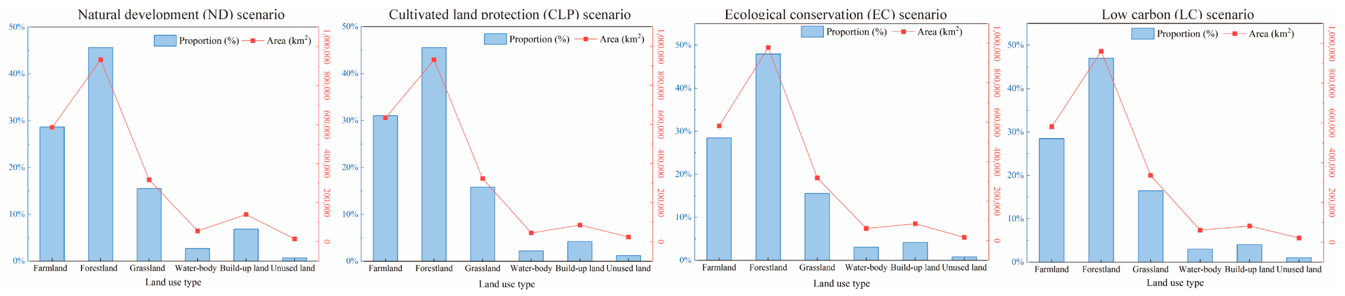
3.1. Land Utilization Pattern under Multi-Scenario Simulations in YREB

The overall layout of land use patterns of the YREB from 2000 to 2020 is shown in Figure 3. To be specific, the land use dynamics encompassed approximately 32.58% and 35.4% of the total expanse of the YREB during the periods spanning from 2000 to 2010 and from 2010 to 2020, respectively. The Kappa coefficient revealed by the authentic land use data in 2020 reached 0.87, while the overall accuracy stood at 94.2%. These results testify to the remarkable congruity between predicted and actual values, thus fortifying the viability of utilizing them for precise prognostication and the insightful analysis of land use patterns in the YREB. The table of the amount of land use type areas under different scenarios is shown in the Supplementary Material (Tables S1–S4). Anticipated land use outcomes for the YREB in 2030 are brought to light in Figure 4 and Figure 5. In accordance with the ND scenario, the area of farmland and grassland decreased by 22,131.42 km² and 8828.21 km², respectively, and the expansion of built-up land is obvious, with an expansion of 69.78%, indicating that without policy restrictions, built-up land will grow rapidly with the intensification of human activities and occupy other types of land such as farmland, forestland, and grassland. In the context of the CLP scenario, forestland decreased from 941151.12 km² to 930497.54 km², the proportion of grassland decreased from 16.04% to 15.82%, and water bodies decreased by 0.28%, while farmland and built-up land will increase. In relation to EC scenario, forestland and built-up land increased by 38493.08 km² and 3183.55 km², respectively. The area of other land use types decreased. Considering the LC scenario, built-up land has expanded to a certain extent, but only increased by 189.54 km². The forestland has increased by 18,865.38 km², accounting for 46.05% to 46.97%, which gives the YREB more significant ecological benefits, and further improves the regional carbon sequestration capacity, which is conducive to the YREB to achieve low-carbon and sustainable development.

3.2. Spatial Pattern of Land Use Carbon Emission

3.2.1. Forecasting the Energy Consumption

By analyzing the statistical data pertaining to eight distinct forms of energy utilization within the YREB region spanning from 2000 to 2020, we have implemented the gray forecast model to accurately project the energy consumption anticipated for the year 2030 (

Table 4. Energy consumption forecast of YREB in 2030.

Energy Type	Energy Consumption/t				Posterior Difference Ratio (C)	Mean Relative Error $\overline{\mathit{\epsilon }}$/%
	2000	2010	2020	2030
run-of-coal	5,556,851	15,693,697	22,519,700	31,499,661	0.023	4.53
coke	580,819	2,085,717	3,048,500	3,760,847	0.033	4.86
gasoline	17,864	13,245	11,343	12,264	0.133	6.19
Crude oil	3,464,925	5,352,902	6,343,200	8,796,598	0.217	7.62
kerosene	978	584	358	312	0.029	17.12
Diesel oil	27,537	43,674	24,732	21,475	0.319	8.35
Fuel oil	369,521	140,540	13,151	1312	0.118	3.42
Natural gas	46,283	162,539	235,211	361,652	0.028	6.07

). The results showed that the posterior difference ratio corresponding to the predicted results of different types of energy consumption is less than 0.35, suggesting a strong concordance between the predicted outcomes and their corresponding measurements, denoting a high degree of fitting precision; the posterior difference ratio test is up to standard. A diminutive relative error, typically below the threshold of 20%, signifies optimal accuracy, that is, the fit is good. Therefore, in general, the relative error is up to standard, the predicted value is close to the original value, and the model prediction results are more reliable.

3.2.2. Land Use Carbon Emission under Multi-Scenario Simulations in YREB

Figure 6 presents the spatial distribution of LUCE intensity in the YREB across various scenarios. Broadly speaking, the LUCE intensity in the YREB exhibits a markedly pronounced development pattern in the central sections of both the Chengdu–Chongqing region and the downstream Yangtze River Delta, regardless of the specific scenarios considered. To be specific, under the CLP scenario, the maximum carbon emission intensity of farmland is 6.65, and under the LC environment scenario, the minimum carbon emission intensity is 4.65, indicating that the cultivated land protection policy can effectively control the protection of farmland area and increase the carbon emission of farmland. Under the EC scenario, returning farmland to grassland and forestland can effectively reduce the farmland carbon emission. The values of forestland, grassland, and water bodies reached −5.53, −5.52, and −3.01, respectively, indicating that forestland, grassland, and water bodies were effectively protected and carbon emission intensity was effectively reduced in the EC scenario. Under the LC scenario, the maximum LUCE of forestland is −6.98, the expansion of built-up land is effectively curbed, and the minimum LUCE is 9.03. Further, the scenario with the lowest LUCEs is the LC scenario, mainly because the expansion of built-up land is greatly reduced, and the forestland is greatly increased. The primary driver behind the LUCE phenomenon within the CLP scenario may well reside in the substantial expansion of urbanized territories, thereby counterbalancing the carbon sequestration potential derived from the simultaneous growth of forestland and grassland areas. This is not only connected with the setting of scenario parameters, but also due to the great influence of uncertainty on the carbon emission coefficient of built-up land. It can be seen that built-up land is the largest contributor to increasing LUCEs, and forestland is the land use type that reduces the influence of LUCEs.

3.3. Spatial Pattern of Ecological Risk in YREB

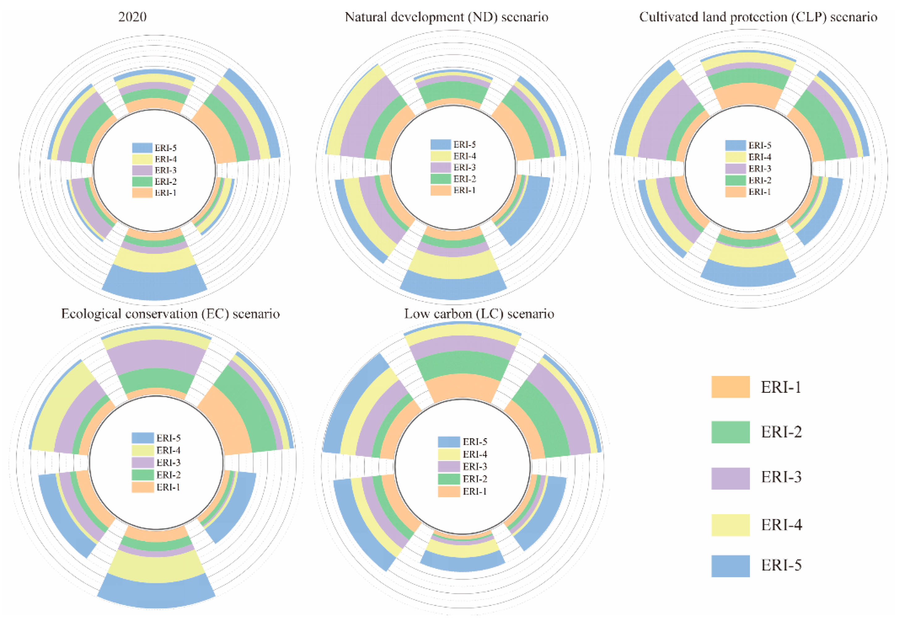
3.3.1. Spatial Pattern of Ecological Risk Index Considering Uncertainty

The performed sensitivity analysis demonstrates that the flexibility of the ERI exhibited a comparatively modest magnitude within four future scenarios, regardless of the assigned probability. Taken as a whole, the ERI exhibited dependability across varying probability-based scenarios. The spatio-temporal patterns of five ESs in the YREB under multi-scenario simulations are in the Supplementary Materials (Figure S1).

Our results demonstrate pronounced spatial heterogeneity in the overall ERI of the YREB (Figure 7). Specifically, in the ND scenario, the conspicuous proliferation of urbanized land within the YREB region is undeniably apparent, encroaching upon vast stretches of farmland, forestland, and grasslands. Consequently, this phenomenon contributes significantly to the heightened ER within the YREB, leading to a critical state of concern. The land use simulation process of the CLP scenario limited the farmland conversion and built-up land expansion caused by the cultivated land protection policy, resulting in a small amount of expansion in the Yangtze River Delta city agglomeration, and in the middle and lower reaches, the degree of mixing of large areas of farmland and forestland was also significantly reduced. Therefore, in contrast to the ND scenario, the ER of the YREB under the CLP scenario is reduced to a certain extent, which may be related to the effective control of the reduction of farmland area and the effective control of the encroachment of forestland and built-up land on farmland. In the EC scenario, the dominant land use types primarily consist of forestland and grassland. The change rate in urbanized land decreases, and the situation of rapid encroachment of urbanized land into ecological land is improved, thus amplifying the decline in the YREB’s ER in the face of the EC scenario. In the LC scenario, the expansion of urbanized land is considerably curtailed, and the expansion rate is much smaller than that in the EC scenario, and the forestland is protected to the greatest extent under this scenario, which minimizes the ER of the YREB.

3.3.2. Ecological Risk Index under Multi-Scenario Simulations in YREB

The resultant classification reveals a discernible elevation in the hierarchical scale of ER, wherein ERI-1 is the lowermost ER, while ERI-5 is the apex of ER (Figure 8). Delving into the specifics, the ERI-1 region predominantly features farmland, encompassing a significant share of 38.76%, followed closely by forestland, which accounts for 18.98% of the land utilization. In contrast, the ERI-2 region exhibits a distinct shift in land use, with forestland and grassland prevailing as the primary types, constituting 25.84% and 26.84%, respectively, while the proportion of forestland remains significantly lower compared to that of ERI-1. Furthermore, building land represents the smallest fraction, merely amounting to 12.76%. Lastly, the ERI-3 region showcases grassland and water bodies as the primary land use types, occupying 25.45% and 25.41%, respectively. Compared with other zones, the proportion of unused land is 2.23%. The most common land types of ERI-4 and ERI-5 are building land, accounting for 35.87% and 53.87%, respectively. In the ERI-4 region, the unused land reached the largest proportion, accounting for 13.54%.

3.4. Interaction Effect Analysis of ERI and LUCE in YREB

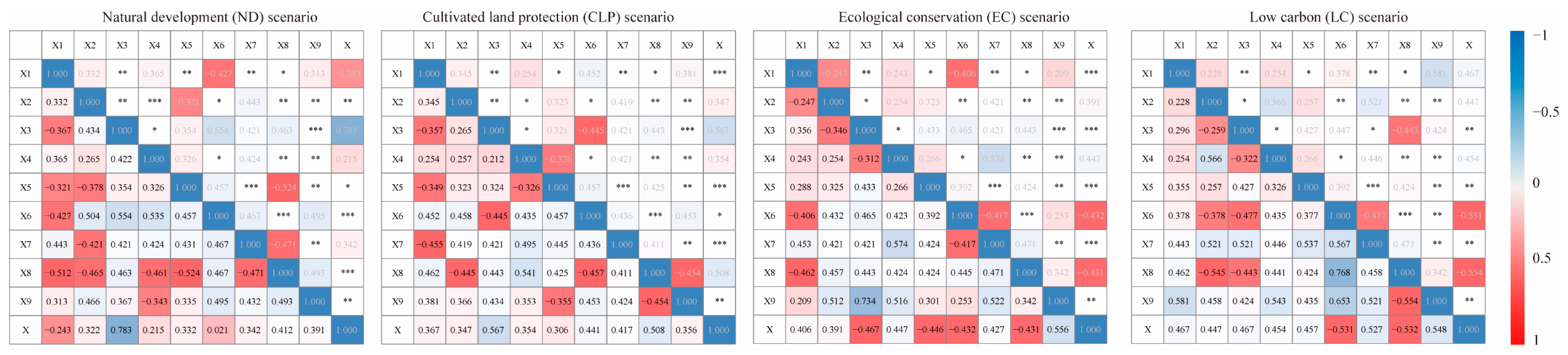
3.4.1. Spatial Spillover Effects Analysis

In four distinct scenarios examined, both the ERI and LUCE variables exhibit a notable presence of spatial autocorrelation, as indicated by the global Moran’s I values (p < 0.001) (

Table 5. Global Moran’s I index of LUCE and ERI.

	ND Scenario	CLP Scenario	EC Scenario	LC Scenario
LUCE	0.8853 ***	0.8533 ***	0.8621 ***	0.8021 ***
z-score	22.2187	19.3325	18.5412	19.4431
p-value	0.0000	0.0000	0.0000	0.0000
ERI	0.7028 ***	0.7932 ***	0.7887 ***	0.7135 ***
z-score	18.1124	18.2235	16.3373	17.9921
p-value	0.0000	0.0000	0.0000	0.0000

Notes: ND is for natural development, CLP is for cultivated land protection, EC is for ecological conservation, LC is for low carbon. *** significant at 1% level.

). Based on the spatial correlation analysis mentioned previously, the ERI and LUCEs were spatially dependent, indicating that the appropriate spatial panel model must be used to avoid biased estimations of the relationship between them. In this study, the LM tests for spatial lag and spatial error were performed based on non-spatial panel models. The LM tests revealed that the null hypothesis of no spatial lag term and no spatial error autocorrelation term were strongly rejected in all the selected models. There were significant spatial effects in the data according to the classic LM tests and robust LM tests; thus, the spatial panel model is superior to the traditional panel model, which lacks spatial effects, because it more effectively combines spatio-temporal distribution characteristics to analyze the spatial response of LUCEs to ERI. The relevant results of the panel model testing are shown in the Supplementary Document (Tables S5–S12).

Table 6. The results of spatial spillover effect.

Variables	ND Scenario			CLP Scenario			EC Scenario			LC Scenario
	SFE	TFE	STFE	SFE	TFE	STFE	SFE	TFE	STFE	SFE	TFE	STFE
LUCE	4.5543 *** (−25.9843)	0.4529 *** (−4.9821)	6.9032 *** (−26.9832)	3.7893 *** (−20.0921)	0.2134 *** (−2.9311)	4.5642 *** (−18.8932)	3.0983 *** (−19.8921)	0.1549 *** (−3.9021)	4.2351 *** (−18.8932)	4.5621 *** (−27.3391)	0.5521 *** (−4.8921)	6.0921 *** (−26.7821)
W * LUCE	2.4609 *** (7.5067)	−0.3414 *** (−3.9846)	2.2818 *** (7.0703)	1.6743 *** (5.9032)	−0.7832 *** (−2.9013)	1.8932 *** (5.9021)	1.8954 *** (6.0921)	−0.2145 *** (−4.9021)	1.4532 *** (6.9021)	2.6701 *** (8.0912)	−0.5732 *** (−5.9921)	2.8901 *** (8.0121)
ρ	−0.9110 *** (97.1879)	−0.9100 *** (97.2978)	−0.8820 *** (68.1151)	−0.8821 *** (88.9012)	−0.8912 *** (87.1286)	−0.7891 *** (77.9012)	−0.7821 *** (83.9901)	−0.7912 *** (80.9045)	−0.7714 *** (63.9012)	−0.9312 *** (102.9012)	−0.9123 *** (105.9034)	−0.9034 *** (78.0932)
R2	0.9659	0.8109	0.9648	0.8878	0.7012	0.7435	0.8012	0.8823	0.8901	0.9023	0.9123	0.8702
σ2	0.0007	0.0173	0.0032	0.0001	0.0214	0.0013	0.0014	0.0002	0.0045	0.0022	0.0023	0.0012
Log-L	2314.4079	837.5126	2334.5706	2125.4462	670.8923	2209.8912	1989.9023	903.8912	2214.9023	2090.3131	987.8912	2289.9012

Notes: SFE: spatial fixed effects. TFE: time period fixed effects. STFE: spatial and time period fixed effects. Log-L: log-likelihood. *** and * represent the statistical significance at the 1%, 5%, and 10% thresholds, respectively. ND is for natural development, CLP is for cultivated land protection, EC is for ecological conservation, and LC is for low carbon.

shows the regression results of spatial spillover effects of LUCE and ERI in the YREB. W* LUCE represents the spatial weight of LUCEs, that is, the weight of the explanatory variable at the X position. ${\sigma }^2$ is the specific error of an individual effect, and the smaller the value, the better the regression fitting. ${\mathrm{R}}^2$ is the coefficient of determination, which represents the degree of fitting of the regression model. The spatial lag coefficients of the four scenarios were ρ = −0.8821, ρ = −0.7891, ρ = −0.7714, and ρ = −0.9034 (p < 0.01), indicating that LUCEs showed significant negative spillover effects under four different scenarios. In other words, according to the SDM results with a spatio-temporal fixed effect, under different scenarios, LUCEs of adjacent administrative units will decrease by 0.8821%, 0.7891, 0.7714, and 0.9034, respectively, for each 1% augmentation in the LUCEs of neighboring administrative units. Furthermore, an analysis of Table 6 reveals a conspicuous negative relation between LUCEs and ERI in the YREB region. This finding suggests that the escalation of LUCEs leads to the deterioration of ERI within the given area. Moreover, our paper proceeds to dissect the spatial impact of LUCEs on ERI using the partial differential method, discerning between its direct and indirect effects. In the ND scenario, the direct effect value of LUCEs on ERI is observed to be −3.7822 (p = 0.0000). This indicates that for each percentage point increase in LUCEs, there is a direct degradation contribution of 3.7822% on ERI. Impressively, the indirect coefficient also demonstrates statistical significance at −4.9012 (p = 0.0000). Intriguingly, the magnitude of the direct effect slightly surpasses that of the indirect affect. This outcome underscores the conspicuous overflow effect of LUCEs from adjacent regions onto the local ERI within our study area. The comprehensive effect (−8.6834, p = 0.0000) exhibited a significant inhibitory impact of LUCEs on ERI within the region. Empirically, a 1% increase in LUCEs led to a decrease in ERI by 8.6834%. Amid the local conditions, the direct coefficient of influence of LUCEs on ERI (−3.0912, p = 0.0000) highlights that the discernible contribution of LUCEs towards ERI degradation amounts to 4.0912% for each 1% rise in LUCEs. Importantly, the indirect effect value also survives the test of significance (−3.2375, p = 0.0000), with the direct impact surpassing the equivalent indirect impact, which underscores the discernible spatial overflow impact of LUCEs in adjacent regions on the local ERI. Finally, the comprehensive impact (−6.3287, p = 0.0000) signifies a substantial inhibitory impact of LUCEs on ERI within the region, as a minute 1% increase in LUCEs initiates a considerable decrease in ERI by 7.9012%.

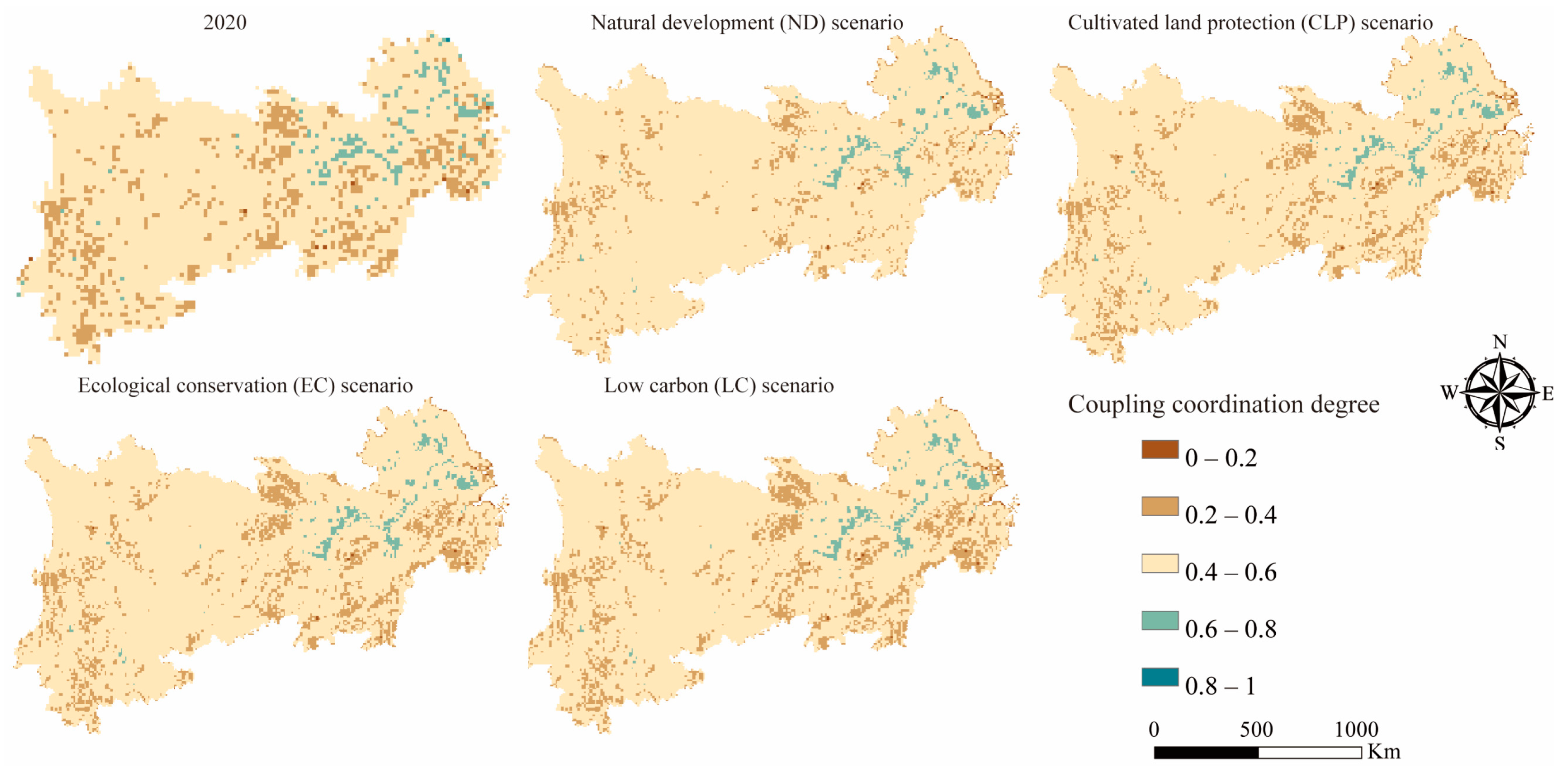
3.4.2. Coupling Coordination Effects Analysis

The findings demonstrate notable spatial heterogeneity in the coordination state of the YREB across various scenarios (Figure 9). In 2030, the spatial allocation of the coupling coordination state in the YREB presents the characteristics of a higher coupling coordination value in the Chengdu–Chongqing city cluster, midstream city cluster, and upstream Yangtze River Delta region. In the ND scenario, unbalanced development is the main type of unbalanced development, which accounts for 87.14%. Compared with the ND scenario, the number of seriously unbalanced development areas in the CLP scenario has increased significantly, and unbalanced development and seriously unbalanced development are the most important coordination types. The proportion was 68.87% and 13.65%, respectively. In the EC scenario, unbalanced development and seriously unbalanced development are still the most important coordination types, but the proportion of unbalanced development increases significantly, accounting for 23.56%. Under the LC scenario, the proportion of moderately balanced development is the largest, reaching 62.78%, and the overall development trend of the YREB becomes better.

4. Discussion

4.1. Further Comprehension of Carbon Emissions with Land Use

In this study, we coupled the PLUS model and gray forecast model to predict LUCEs in different scenarios in the future, which makes up for the defect that the carbon emission coefficient method used in the previous research on LUCEs fails to combine future LUCEs with the past timeline and conduct spatio-temporal simulations. Based on the findings of our analysis, it can be deduced that within the realm of LUCEs, carbon emissions originating from urbanized areas comprise the predominant portion of the overall net carbon emissions, which corroborates the fundamental role attributed to urbanized regions, as evidenced by prior investigations. Furthermore, given that carbon emissions from urbanized areas predominantly emanate from energy consumption related to human activities, the gray forecast model has been employed to forecast future energy consumption and subsequently estimate future carbon emissions, which has important reference value for forecasting the future carbon emission trajectory of the region. In addition, the study extracted nine key determinants from the interaction of natural ecosystems and socio-economic frameworks (Figure 10). The transformation of grasslands is predominantly influenced by meteorological elements such as precipitation and temperature, accounting for a remarkable 55.9% contribution. When analyzing alterations in forested areas, the interplay between precipitation and slope emerges as the principal driving force, encompassing 53.4% of the total impact. In recent years, the YREB region has implemented the policy of farmland protection, while the YREB has also taken measures to return farmland to grassland and forestland. According to the EC scenario of this study, the proper conversion of farmland to grassland and forestland plays a certain role in ecological restoration. In the LC scenario, controlling and reducing the consumption of fossil energy while protecting the carbon absorbing land such as forestland and grassland will contribute in a beneficial manner to the harmonious and sustainable progress of carbon mitigation and ecological revitalization in the YREB region.

4.2. Comprehensive Analysis of Ecological Risk Considering Land Utilization

The ER encompasses the evaluation of the possible ramifications that human endeavors may have on the vitality and equilibrium of ecosystems and their constituents [32]. The depletion of ecosystems attributed to human activities must be regarded as a latent peril, one that imperils the very fabric of these intricate systems [33]. Consequently, this study endeavors to quantify forthcoming uncertainties through the adoption of simulation techniques employing multiple scenarios. Furthermore, the utilization of gains and losses in the measurement of ecosystem service values (ESVs) can effectively guide the allocation of conservation efforts and management practices, especially in the face of constrained resources. To be specific, in the EC scenarios, the ESVs of all services on the YREB is relatively high. In the context of the ND scenario, with the progressive urbanization, the augmentation of built-up land trumps that of water bodies, thereby exacerbating the ecological vulnerability in the eastern region of the YREB. The ER in this area is further intensified by the relentless encroachment of human activities and the resultant land utilization patterns.

The influencing factors of the ERI of the YREB are shown in Figure 11. In the ND scenario, slope, temperature, and GDP all pass the significance test, which indicates that the ERI will be influenced by both natural and human factors along with the current natural development trajectory. In the CLP scenario, precipitation also passed the significance test, which may be related to the fact that there are more rivers, lakes, and other water bodies in the YREB region. In the EC scenario, the ERI has more significant changes in precipitation and temperature, but less significant changes in GDP. In the LC scenario, considering the uncertainty of the ESV in the YREB region, this study further found that the ERI was negatively correlated with population and GDP, and positively correlated with temperature, precipitation, and slope. The analysis of the ND scenario and EC scenario reveals that notable strides in the transformation of farmland into forestland and the successful implementation of a range of policies aimed at safeguarding the delicate ecological equilibrium in the upper stretches of the YREB have been made. In the lower reaches of the river, namely Jiangsu, Zhejiang, and other localities, there exists a condensed clustering of areas witnessing a shift from cultivated land to urbanized landscapes. Additionally, a series of minor aggregation conversion centers have emerged in the middle regions of the YREB and surrounding the Chengdu–Chongqing city agglomeration. The predominant factor lies in the relentless enhancement of development strategies pertaining to urban clusters. Amidst the external progression of urban clusters, the periphery surrounding the suburban vicinities has emerged as the principal trajectory for urban expanding. Consequently, arable land has evolved into the key auxiliary reservoir of built-up land. Thus, the ER in the southwestern domain of the YREB has undergone marked alleviation. This juxtaposition effectively elucidates the disparities between regions within the YREB and provides valuable insights for devising policies aimed at risk mitigation.

4.3. Interaction Effect and Policy Implications

The transformation in the land utilization structure, prompted by the interplay of natural, economic, and social factors [34], fundamentally shapes the alterations observed in the ecological environment within the YREB. The distribution characteristics of land use structure are predominantly shaped by the inherent attributes of the natural ecological milieu, while the socio-economic agenda effectively governs the magnitude and direction of land use changes [35]. The progressive expansion of urbanized areas in the YREB region has significantly encroached upon cultivated and ecological lands, resulting in a particularly precipitous decline in the extent of cultivated land. This process has induced intricate and interdependent modifications among various regions, owing to the dual demands of human development and the implementation of protective ecological policies. The spatial heterogeneity of clustering patterns emerges when observing the contrasting distributions of LUCEs and ER across four distinct scenarios. Notably, the agglomeration of high–low values predominantly occurs in the northeast region of the YREB, specifically in the lower stretches of the YREB. These administrative divisions demonstrate a remarkable interconnection, with both urban agglomerations exhibiting a higher regional economic development level and elevated LUCEs. Conversely, the assemblage of low–high values predominantly materializes in the northwestern expanse, which encompasses the upper reaches of the YREB. These areas boast abundant forest resources and intricate water systems that contribute to rich ecosystem services. Consequently, ER experiences a significant reduction.

Therefore, measures should be taken in accordance with the actual situation in each region. Efforts should be made to strengthen ecological protection and restoration in upstream areas and improve water conservation capacity [36]. After 2000, the expanse of forested and grassy domains in YREB has witnessed a marked increment. However, the pernicious affliction of desertification remains a grave predicament, jeopardizing the very fabric of ecological stability [37]. Therefore, it is particularly important that on the basis of the existing forestland and grassland, the overdevelopment of ecological land should be controlled, the process of natural vegetation restoration should be accelerated, and the coverage rate of forest land should be expanded, so as to effectively curb the trend of ecological degradation in the upstream area, improve the capacity of water conservation, and maintain biodiversity [38]. Efforts should be made to prevent and control soil erosion in the middle reaches and improve soil and water conservation capacity [39]. The most important problem facing the middle reaches of the YREB is serious soil erosion. We will speed up capacity building for forest land and grassland protection and water and soil conservation, and implement ecological protection measures in light of local conditions. We will continue to consolidate the project to return farmland to forests and grasslands, and effectively expand forest and grassland area [40]. With the advancement of urbanization in the downstream region of the YREB, the population continues to gather, and the expansion speed of built-up land continues to accelerate, resulting in sharp contradictions between farmland and built-up land [41]. It becomes imperative to prioritize a judicious and intensive utilization of land resources, while simultaneously curbing the alarming rate of farmland depletion and mitigating the unrestrained proliferation of built-up areas. Thus, the downstream Yangtze River Delta is an ecologically fragile area, so it is necessary to strengthen ecological protection in the delta area, strengthen forest and grass protection measures, and promote ecological comprehensive improvement.

5. Conclusions

In light of the examination surrounding prospective uncertainties, this study anticipated the LUCEs and ERI under varied scenarios. Moreover, it delved into the interplay between LUCEs and ERI, investigating the spatial spillover effect and bidirectional coupling response.

When contrasting the spatial allocation of land utilization across the YREB amidst four discrete scenarios, under the CLP scenario, an effective control is exerted over the reduction of cultivated land. The LC scenario observes a notable decrease in the proliferation of built-up land, a striking juxtaposition to the conspicuous expansion witnessed in the EC scenario. In the realm of LC scenarios, a remarkable reduction in the LUCEs of forestland was observed, effectively curbing the expansion of construction land. It is noteworthy that construction land emerges as the paramount contributor to the escalation of carbon emissions resulting from land use, whereas forest land emerges as a mitigating force, effectively countering the impact of such emissions. Across the four examined scenarios, discernible spatial heterogeneity emerges in the ERI within the YREB. It reveals a substantial decline in the expansion of construction land in the LC scenario, which is notably more limited compared to the EC scenario. In different scenarios, the presence of LUCEs exhibits a substantial adverse spillover impact on the ERI, and the bidirectional spatial coupling effect between LUCEs and ERI is significantly different. The ND scenario demonstrates the lowest CCD, while the LC scenario exhibits the highest level of CCD.

References

1. Cao, M.; Chang, L.J.; Ma, S.J.; Zhao, Z.J.; Wu, K.; Hu, X.; Gu, Q.S.; Lü, G.N.; Chen, M. Multi-Scenario Simulation of Land Use for Sustainable Development Goals. IEEE J. Sel. Top. Appl. Earth Obs. Remote Sens. 2022, 15, 2119–2127. [Google Scholar] [CrossRef]
2. Warchold, A.; Pradhan, P.; Thapa, P.; Putra, M.P.I.F.; Kropp, J.P. Building a unified sustainable development goal database: Why does sustainable development goal data selection matter? Sustain. Dev. 2022, 30, 1278–1293. [Google Scholar] [CrossRef]
3. Xu, Q.; Dong, Y.X.; Yang, R.; Zhang, H.O.; Wang, C.J.; Du, Z.W. Temporal and spatial differences in carbon emissions in the Pearl River Delta based on multi-resolution emission inventory modeling. J. Clean. Prod. 2019, 214, 615–622. [Google Scholar] [CrossRef]
4. Gao, L.; Wen, X.; Guo, Y.T.; Gao, T.M.; Wang, Y.; Shen, L. Spatiotemporal Variability of Carbon Flux from Different Land Use and Land Cover Changes: A Case Study in Hubei Province, China. Energies 2014, 7, 2298–2316. [Google Scholar] [CrossRef]
5. Sinha, A.; Sengupta, T.; Alvarado, R. Interplay between technological innovation and environmental quality: Formulating the SDG policies for next 11 economies. J. Clean. Prod. 2020, 242, 118549. [Google Scholar] [CrossRef]
6. Xu, T.; Zhang, M.; Gao, L.J.; Yang, B.; Shi, L.Y. Development and application of a comprehensive ecological risk assessment indicator system in Xiamen, China. Int. J. Sustain. Dev. World Ecol. 2018, 25, 468–476. [Google Scholar] [CrossRef]
7. Qu, Z.; Zhao, Y.H.; Luo, M.Y.; Han, L.; Yang, S.Y.; Zhang, L. The Effect of the Human Footprint and Climate Change on Landscape Ecological Risks: A Case Study of the Loess Plateau, China. Land 2022, 11, 217. [Google Scholar] [CrossRef]
8. Ju, H.R.; Niu, C.Y.; Zhang, S.R.; Jiang, W.; Zhang, Z.H.; Zhang, X.L.; Yang, Z.Y.; Cui, Y.R. Spatiotemporal patterns and modifiable areal unit problems of the landscape ecological risk in coastal areas: A case study of the Shandong Peninsula, China. J. Clean. Prod. 2021, 310, 127522. [Google Scholar] [CrossRef]
9. Qu, Y.B.; Zong, H.N.; Su, D.S.; Ping, Z.L.; Guan, M. Land Use Change and Its Impact on Landscape Ecological Risk in Typical Areas of the Yellow River Basin in China. Int. J. Environ. Res. Public Health 2021, 18, 11301. [Google Scholar] [CrossRef]
10. Tang, L.; Ma, W. Assessment and management of urbanization-induced ecological risks. Int. J. Sustain. Dev. World Ecol. 2018, 25, 383–386. [Google Scholar] [CrossRef]
11. Xu, Q.; Guo, P.; Jin, M.T.; Qi, J.F. Multi-scenario landscape ecological risk assessment based on Markov-FLUS composite model. Geomat. Nat. Hazards Risk 2021, 12, 1448–1465. [Google Scholar] [CrossRef]
12. Sun, N.S.; Chen, Q.; Liu, F.G.; Zhou, Q.; He, W.X.; Guo, Y.Y. Land Use Simulation and Landscape Ecological Risk Assessment on the Qinghai-Tibet Plateau. Land 2023, 12, 923. [Google Scholar] [CrossRef]
13. Gao, P.; Yue, S.J.; Chen, H.T. Carbon emission efficiency of China’s industry sectors: From the perspective of embodied carbon emissions. J. Clean. Prod. 2021, 283, 124655. [Google Scholar] [CrossRef]
14. Wang, Q.; Yang, X. Imbalance of carbon embodied in South-South trade: Evidence from China-India trade. Sci. Total Environ. 2020, 707, 134473. [Google Scholar] [CrossRef] [PubMed]
15. Chuai, X.W.; Huang, X.J.; Wang, W.J.; Zhao, R.Q.; Zhang, M.; Wu, C.Y. Land use, total carbon emission’s change and low carbon land management in Coastal Jiangsu, China. J. Clean. Prod. 2015, 103, 77–86. [Google Scholar] [CrossRef]
16. Zhang, D.; Wang, Z.Q.; Li, S.C.; Zhang, H.W. Impact of Land Urbanization on Carbon Emissions in Urban Agglomerations of the Middle Reaches of the Yangtze River. Int. J. Environ. Res. Public Health 2021, 18, 1403. [Google Scholar] [CrossRef] [PubMed]
17. Arora, A.; Pandey, M.; Mishra, V.N.; Kumar, R.; Rai, P.K.; Costache, R.; Punia, M.; Di, L.P. Comparative evaluation of geospatial scenario-based land change simulation models using landscape metrics. Ecol. Indic. 2021, 128, 107810. [Google Scholar] [CrossRef]
18. Lin, J.Y.; Li, X.; Wen, Y.Y.; He, P.T. Modeling urban land-use changes using a landscape-driven patch-based cellular automaton (LP-CA). Cities 2023, 132, 103906. [Google Scholar] [CrossRef]
19. Zheng, F.Y.; Hu, Y.C. Assessing temporal-spatial land use simulation effects with CLUE-S and Markov-CA models in Beijing. Environ. Sci. Pollut. Res. 2018, 25, 32231–32245. [Google Scholar] [CrossRef]
20. Liang, X.; Guan, Q.F.; Clarke, K.C.; Liu, S.S.; Wang, B.Y.; Yao, Y. Understanding the drivers of sustainable land expansion using a patch-generating land use simulation (PLUS) model: A case study in Wuhan, China. Comput. Environ. Urban Syst. 2021, 85, 101569. [Google Scholar] [CrossRef]
21. Zeng, Y.S.; Bi, C.J.; Jia, J.P.; Deng, L.; Chen, Z.L. Impact of intensive land use on heavy metal concentrations and ecological risks in an urbanized river network of Shanghai. Ecol. Indic. 2020, 116, 106501. [Google Scholar] [CrossRef]
22. Fitts, L.A.; Russell, M.B.; Domke, G.M.; Knight, J.K. Modeling land use change and forest carbon stock changes in temperate forests in the United States. Carbon Balance Manag. 2021, 16, 20. [Google Scholar] [CrossRef] [PubMed]
23. Wei, Q.; Abudureheman, M.; Halike, A.; Yao, K.-F.; Yao, L.; Tang, H.; Tuheti, B. Temporal and spatial variation analysis of habitat quality on the PLUS-InVEST model for Ebinur Lake Basin, China. Ecol. Indic. 2022, 145, 109632. [Google Scholar] [CrossRef]
24. Wang, Q.; Guan, Q.; Sun, Y.; Du, Q.; Xiao, X.; Luo, H.; Zhang, J.; Mi, J. Simulation of future land use/cover change (LUCC) in typical watersheds of arid regions under multiple scenarios. J. Environ. Manag. 2023, 335, 117543. [Google Scholar] [CrossRef] [PubMed]
25. Wei, H.; Xiong, L.Y.; Tang, G.A.; Strobl, J.; Xue, K.K. Spatial-temporal variation of land use and land cover change in the glacial affected area of the Tianshan Mountains. Catena 2021, 202, 105256. [Google Scholar] [CrossRef]
26. Meneses, B.M.; Reis, E.; Reis, R.; Vale, M.J. The Effects of Land Use and Land Cover Geoinformation Raster Generalization in the Analysis of LUCC in Portugal. Isprs Int. J. Geo-Inf. 2018, 7, 390. [Google Scholar] [CrossRef]
27. Xing, L.; Hu, M.S.; Wang, Y. Integrating ecosystem services value and uncertainty into regional ecological risk assessment: 29. A case study of Hubei Province, Central China. Sci. Total Environ. 2020, 740, 140126. [Google Scholar] [CrossRef] [PubMed]
28. LeSage, J.P. Introduction to Spatial Econometrics; CRC: New York, NY, USA, 2009. [Google Scholar]
29. Zhang, S.H.; Zhong, Q.L.; Cheng, D.L.; Xu, C.B.; Chang, Y.N.; Lin, Y.Y.; Li, B.Y. Landscape ecological risk projection based on the PLUS model under the localized shared socioeconomic pathways in the Fujian Delta region. Ecol. Indic. 2022, 136, 108642. [Google Scholar] [CrossRef]
30. Zheng, L.; Wang, Y.; Li, J.F. Quantifying the spatial impact of landscape fragmentation on habitat quality: A multi-temporal dimensional comparison between the Yangtze River Economic Belt and Yellow River Basin of China. Land Use Policy 2023, 125, 106463. [Google Scholar] [CrossRef]
31. Li, C.; Wu, Y.M.; Gao, B.P.; Zheng, K.J.; Wu, Y.; Li, C. Multi-scenario simulation of ecosystem service value for optimization of land use in the Sichuan-Yunnan ecological barrier, China. Ecol. Indic. 2021, 132, 108328. [Google Scholar] [CrossRef]
32. Baltagi, B.H.; Heun Song, S.; Cheol Jung, B.; Koh, W. Testing for serial correlation, spatial autocorrelation and random effects using panel data. J. Econom. 2007, 140, 5–51. [Google Scholar] [CrossRef]
33. Xie, N.M. A summary of grey forecasting models. Grey Syst. Theory Appl. 2022, 12, 703–722. [Google Scholar] [CrossRef]
34. Zhang, S.; Wu, T.; Guo, L.; Zou, H.; Shi, Y. Integrating ecosystem services supply and demand on the Qinghai-Tibetan Plateau using scarcity value assessment. Ecol. Indic. 2023, 147, 109969. [Google Scholar] [CrossRef]
35. Wei, L.L.; Zhang, C.L.; Su, J.J.; Yang, L.X. Panel threshold spatial Durbin models with individual fixed effects. Econ. Lett. 2021, 201, 109778. [Google Scholar] [CrossRef]
36. Pan, Z.Z.; He, J.H.; Liu, D.F.; Wang, J.W.; Guo, X.A. Ecosystem health assessment based on ecological integrity and ecosystem services demand in the Middle Reaches of the Yangtze River Economic Belt, China. Sci. Total Environ. 2021, 774, 144837. [Google Scholar] [CrossRef]
37. Zhang, W.; Liu, G.Y.; Yang, Z.F. Urban agglomeration ecological risk transfer model based on Bayesian and ecological network. Resour. Conserv. Recycl. 2020, 161, 105006. [Google Scholar] [CrossRef]
38. Zhang, X.M.; Du, H.M.; Wang, Y.; Chen, Y.; Ma, L.; Dong, T.X. Watershed landscape ecological risk assessment and landscape pattern optimization: Take Fujiang River Basin as an example. Hum. Ecol. Risk Assess. 2021, 27, 2254–2276. [Google Scholar] [CrossRef]
39. Wang, N.; Zhu, P.J.; Zhou, G.H.; Xing, X.D.; Zhang, Y. Multi-Scenario Simulation of Land Use and Landscape Ecological Risk Response Based on Planning Control. Int. J. Environ. Res. Public Health 2022, 19, 14289. [Google Scholar] [CrossRef]
40. Ran, P.L.; Hu, S.G.; Frazier, A.E.E.; Qu, S.J.; Yu, D.; Tong, L.Y. Exploring changes in landscape ecological risk in the Yangtze River Economic Belt from a spatiotemporal perspective. Ecol. Indic. 2022, 137, 108744. [Google Scholar] [CrossRef]
41. Chen, S.; Li, G.; Zhuo, Y.F.; Xu, Z.G.; Ye, Y.M.; Thorn, J.P.R.; Marchant, R. Trade-offs and synergies of ecosystem services in the Yangtze River Delta, China: Response to urbanizing variation. Urban Ecosyst. 2022, 25, 313–328. [Google Scholar] [CrossRef]
Figure 1. (a) The location of the area; (b) map of the area; (c) the DEM of the area; and (d) the land use type in 2020.
Land 13 00937 g001
Figure 2. Research framework.
Land 13 00937 g002
Figure 3. The dynamic patterns of land utilization evolution of 2000–2020.
Land 13 00937 g003
Figure 4. Land use predictions under multi-scenario simulations in YREB.
Land 13 00937 g004
Figure 5. Land use type area under different scenarios.
Land 13 00937 g005
Figure 6. LUCE predictions under multi-scenario simulations in YREB.
Land 13 00937 g006
Figure 7. Spatial distribution of ERI under multi-scenario simulations in YREB.
Land 13 00937 g007
Figure 8. Proportion of ecological risk index by land use types (ERI: ecological risk index).
Land 13 00937 g008
Figure 9. Coupling coordination degree changes in YREB under multi-scenario simulations.
Land 13 00937 g009
Figure 10. Contribution of different factors to land se carbon emission.
Land 13 00937 g010
Figure 11. Driving factors of ecological risk index (X1: Dis-water, X2: Dis-Railway, X3: Slop, X4: Dis-Traffic, X5: Temperature, X6: Population, X7: Precipitation, X8: GDP, X9: DEM, X: ERI). ***, **, and * represent the statistical significance at the 1%, 5%, and 10% thresholds correspondingly.).
Land 13 00937 g011