Soil Quality Assessment and Its Spatial Variability in an Intensively Cultivated Area in India

Abstract

Intensive agricultural practices lead to a deterioration in soil quality, causing a decline in farm productivity and quality, and disturbing the ecosystem balance in command areas. To achieve sustainable production and implement effective soil management strategies, understanding the state and spatial variability of soil quality is essential. The study aims to enhance the understanding of soil quality variability and provide actionable insights for sustainable soil management. In this regard, principal component analysis (PCA) and digital soil mapping were used to assess and map the spatial variability of the soil quality index (SQI) in the Cauvery command area, Mandya district, Karnataka, India. A total of 145 georeferenced soil samples were drawn at 0–15 cm depth and analyzed for physico-chemical properties. PCA was used to reduce the dataset into a minimum dataset as eight important soil indicators and to determine relative weightage factors, which were used for assessing SQI with linear and non-linear scoring methods. For spatial assessment of SQI, the random forest algorithm with environmental covariates was used to map eight soil indicators selected in the minimum dataset. The soil property maps were subjected to linear and non-linear scoring, followed by multiplying with corresponding weightage factors and summation to produce SQI maps. Results reveal that values of SQI calculated using linear scoring, range from 0.10 to 0.64, with a mean of 0.39, while non-linear scoring exhibits a wider range of 0.12 to 0.78 and a mean of 0.48. With a slight higher sensitivity index of 6.5, non-linear scoring proved to be the better scoring method compared to linear scoring. Spatial assessment shows that the R² and LCC between the calculated and predicted SQI were higher for non-linear scoring (0.66 and 0.66) compared to linear scoring (0.60 and 0.65). The SQI maps reveal high spatial variability with more than 40 percent of soils classified as moderate-to-low index. The soils with low SQI were distributed in eastern parts, whereas western parts exhibited high-to-very-high soil quality. To achieve production goals and improve soil quality in the eastern region, sustainable soil and crop management strategies must be developed, and their effects on soil quality should be assessed.

1. Introduction

In the present era of intensive farming, the most critical problem agricultural landscapes face is maintaining the complex equilibrium between ecosystem and soil functions [1,2]. Sustaining soil fertility while assuring higher food production to meet the demands of the ever-increasing population is an increasing concern [3,4]. In India, command areas have gained importance because of their ability to provide a continuous irrigation water supply through dams, reservoirs, and complex canal networks [5]. By mitigating the risks associated with rainfall uncertainty, the importance of command areas extends beyond agricultural productivity to encompass broader goals such as rural livelihood and food security.

Command areas, despite playing a critical role in agricultural development, often require support with a variety of issues that can significantly impact farm sustainability and productivity [6]. The challenges in the intensively cultivated land under command area include soil pollution, declining soil fertility, erosion, and salinity [7]. Unscientific water management with poor drainage leads to the development of salt-affected soils [8], preventing plant growth and eventually lowering crop yields [7]. Mechanized farming and mono-cropping are intensive agricultural practices that accelerate soil erosion and destroy the ecosystem by removing productive topsoil [9]. Poor soil management during continuous intensive cultivation has resulted in nutritional imbalances in crops, loss of organic matter, and soil compaction, all of which may deteriorate the health and productivity of the soil [8]. The Cauvery command region in southern India is facing issues related to soil quality. Therefore, assessing soil quality is essential for understanding the health and fertility of the soil, guiding proper management practices, and ultimately enhancing agricultural productivity and sustainability [10].

Soil quality is influenced by various physical, chemical, and biological soil properties. Consequently, a thorough assessment of soil quality should encompass variables that accurately reflect soil health and productivity [11]. However, to ensure practicality and efficiency, limiting the number of selected variables is essential. To address the challenge, Andrews et al. [12] proposed a three-tier-based conceptual model containing indicator selection, indicator scoring, and score integration into an index. Various researchers have used [1,11,12,13,14,15] the principal component analysis (PCA) technique to identify the key factors influencing the soil quality index (SQI) and construct a minimum dataset (MDS). Subsequently, these indicators will be transformed into scores ranging between 0 and 1, using linear and non-linear methods [13,14,15,16]. Then, a communality-based weighted additive approach is employed to amalgamate dimensionless indicator scores into comprehensive soil quality indices [17,18].

Soil properties vary spatially, and so does the SQI. Hence, mapping soil quality is essential in identifying the soils with low SQI and prioritizing the zones for sustainable management practices [14,19]. Conventional methods are costly because field sampling, followed by lab analysis, is time-consuming and labor-intensive. Digital soil mapping (DSM) techniques employing machine learning algorithms and environmental variables have the potential to overcome these challenges faced by conventional methods [20]. This technique follows the “SCORPAN” model of McBratney et al. [21], which uses various auxiliary remote sensing data that explain various soil-forming factors and processes. In recent years, various machine learning algorithms, such as random forest [22,23,24,25,26], support vector machine [19,27,28,29], neural networks [30,31,32], and logistic regression [33], have been used to establish a connection between soil properties and SCORPAN variables. Predicted soil property maps can be used for SQI mapping after transforming them into dimensionless units [28,34].

A comprehensive understanding of spatial variability of soil quality in the Cauvery command area aids in prioritizing areas with poor soil quality for targeted interventions aimed at improving soil health and thereby enhancing crop productivity and living standards of rural communities in the area. Therefore, this study aims to advance the understanding of soil quality variability in the Cauvery command area by integrating advanced analytical techniques. Specifically, PCA and scoring methods were employed to assess SQI and conduct spatial mapping using a random forest algorithm and environmental variables.

2. Materials and Methods

2.1. Study Area

The study area is situated in the southern part of Karnataka state, India, covering 91,000 ha of area (12°17′26.26″ N to 12°34′37.64″ N and 76º37′34.26″ E to 77°13′48.33″ E). It is a part of the Cauvery command area receiving irrigation from Krishnaraja Sagara reservoir, with the elevation varying from 561 m to 930 m above MSL. The area exhibits a sub-parallel and dendritic configuration of drainage patterns, resulting in distinct lowlands, midlands, and upland relief characteristics. The study area experiences a semi-arid climate characterized by an average annual rainfall of 770 mm, a mean temperature of 31 °C, potential evapotranspiration (PET) of 1794 mm, and relative humidity ranging from 23% to 89%. The soils in the area are classified as Entisols, Alfisols, and Inceptisols [35], with a hyperthermic temperature regime. The predominant geological formations consist of granite and granite gneiss [36]. Agriculture in the region is dominated by high-water-demanding crops such as sugarcane and paddy.

2.2. Soil Sampling and Analysis

A random soil sampling strategy was employed during March 2023 to ensure a broad understanding of soil quality across the study area. A total of 145 soil samples were collected at 0–15 cm depth from various landscapes with corresponding GPS coordinates. The study area and location of soil samples are depicted in Figure 1. The collected soil samples were subjected to laboratory analyses to determine physico-chemical properties for assessing soil quality. Standard protocols, as described by Jackson, M L [37], were followed for measuring pH, electrical conductivity (EC), bulk density (BD), and maximum water-holding capacity (MWHC). Exchangeable cations (Ca, Mg, Na, K), sodium adsorption ratio (SAR), and cation exchange capacity (CEC) were assessed using the methods outlined by Pansu et al. [38]. Available phosphorus (Avl. P₂O₅) was assessed as per Olsen and Frank [39]. Soil organic carbon (SOC) was estimated following the procedures provided by Walkley, 1947 [40].

2.3. Assessment of Soil Quality Index (SQI)

2.3.1. Minimum Dataset

Andrews et al. [12] described a multivariate statistics-based PCA technique to select soil quality indicators and create a MDS. It comprises variables that are uncorrelated to each other, and the process reduces the multicollinearity of the dataset. In the present study, 12 soil attributes possessing pivotal roles in determining soil health and crop productivity were selected, which include pH, electrical conductivity (EC), organic carbon (OC), available phosphorous (Avl. P₂O₅), potassium (K), calcium (Ca), magnesium (Mg), sodium (Na), sodium adsorption ratio (SAR), maximum water-holding capacity (MWHC), bulk density (BD), and cation exchange capacity (CEC). These critical parameters were selected due to their significant impact on soil fertility, root growth, soil porosity, structure, and aggregate stability [41,42,43]. The soils of the Cauvery command area are prone to soil salinity and alkalinity [44]. Therefore, proxies for salinity, including electrical conductivity (EC), sodium (Na), and sodium adsorption ratio (SAR), were considered for the analysis. The dataset underwent PCA to distill and pinpoint the essential indicators for the MDS.

Principal components (PCs) with eigenvalues ≥1, representing at least 5 percent of the variance, were retained for further analysis [12]. The careful selection process extended to indicators exhibiting high loadings, with threshold values within 90% of the highest loading factor, making them suitable choices for inclusion in the MDS [45]. Given that PCs inherently contain correlated variables, Pearson’s correlation analysis was employed to identify and manage redundancy among attributes within each PC [46]. Specifically, if multiple attributes with high loading factors (greater than the threshold) were present within a PC, those with significant correlations (r > 0.7) were scrutinized. In such cases, priority was given to the attribute with the highest factor loading. The procedure ensured that the MDS comprised a refined selection of soil indicators, emphasizing their non-redundancy and significance in delineating soil quality dynamics.

This selection and evaluation process is integral to the reliability and comprehensiveness of the SQI, as it ensures that only the most influential and non-redundant soil attributes contribute to the overall assessment [47]. The steps followed for SQI calculation are presented in Figure 2.

2.3.2. Scoring of Indicator Soil Properties

Scores were assigned based on the ‘more is better’, ‘less is better’, and ‘optimum range’ functions. The classification of soil quality parameters into “more is better”, “less is better”, and “optimum range” is based on various agronomic principles [48]. Parameters like organic carbon (OC), cation exchange capacity (CEC), available phosphorus (P₂O₅), exchangeable cations (Ca, Mg, K), and maximum water-holding capacity fall under the “more is better” criterion because higher levels of these parameters enhance soil structure, nutrient retention, and overall soil fertility. Conversely, parameters such as sodium adsorption ratio (SAR) and exchangeable sodium (Na) are classified as “less is better” because high levels of sodium can degrade soil structure and reduce permeability. Parameters like electrical conductivity (EC) and pH are classified under the “optimum range” criterion, as both high and low extremes can adversely affect nutrient availability and plant growth [49,50].

Two types of scoring methods, viz., linear scoring (LS) and non-linear scoring (NLS), were followed for transforming soil data into dimensionless units.

(i)

Linear scoring—The indicator scores were assigned based on the ‘more is better’ and ‘less is better’ criteria using linear scoring equations (Equations (1) and (2)) as described by Biswas et al. [51]:

$$\mathbf{L}\mathbf{S}=\frac{\mathbf{V}\mathbf{i}-\mathbf{M}\mathbf{i}\mathbf{n}}{\mathbf{M}\mathbf{a}\mathbf{x}-\mathbf{M}\mathbf{i}\mathbf{n}}$$

(1)

$$\mathbf{L}\mathbf{S}=\frac{\mathbf{M}\mathbf{a}\mathbf{x}-\mathbf{V}\mathbf{i}}{\mathbf{M}\mathbf{a}\mathbf{x}-\mathbf{M}\mathbf{i}\mathbf{n}}$$

(2)

LS is the linearly normalized score for the i^th soil attribute, Vi is the observed value of the i^th soil property, Min is the minimum observed value of the i^th soil property, and Max is the maximum observed value of the i^th soil property.

(ii)

Non-linear scoring—The non-linear scoring of variables was and carried out a sigmoidal type function, as outlined in Equation (3), following the methodologies proposed in various studies [50,52,53]:

$$\mathbf{N}\mathbf{L}\mathbf{S}=\frac{\mathbf{1}}{\mathbf{1}+{\left(\mathbf{V}\mathbf{i}/\mathbf{V}\mathbf{m}\right)}^{\mathbf{b}}}$$

(3)

Vi is the observed value of the i^th soil attribute, Vm is the mean of the i^th soil attribute, and the parameter “b” in the equation represents the slope of the sigmoidal curve. For the ‘more is better’ situation, the value of “b” was set to −2.5, while for the ‘less is better’ state, it was assigned a value of +2.5, defining the steepness and direction of the curve.

These scoring equations standardize the soil property values, transforming them into a dimensionless score between 0 and 1. The ‘more is better’ scoring approach infers that higher values of the soil attribute are desirable, while the ‘less is better’ scoring approach suggests that lower values are desirable.

2.3.3. Development of Soil Quality Indices

To compute soil quality indices using both the scoring methods, the weightage of variables was executed through PCA, employing commonality as a basis [30]. The commonality of each factor elucidated a specific percentage of the variation within the MDS. The weight values assigned to individual indicators were derived from the ratio of the commonality of each quality indicator to the sum of all indicator communalities included in the MDS, following the methodology proposed by Nabiollahi et al. [51]. Then, each indicator’s linear and non-linear scores were multiplied with the weightage factor obtained through commonalities, to obtain LS-SQI and NLS-SQI (Equations (4) and (5)).

$$\mathrm{L}\mathrm{S}\text{-}\mathrm{S}\mathrm{Q}\mathrm{I}=\sum _{\mathrm{i}=1}^{\mathrm{n}}\mathrm{W}\mathrm{i}\ast \mathrm{L}\mathrm{S}\mathrm{i}$$

(4)

$$\mathbf{N}\mathbf{L}\mathbf{S}\text{-}\mathbf{S}\mathbf{Q}\mathbf{I}=\sum _{\mathbf{i}=\mathbf{1}}^{\mathbf{n}}\mathbf{W}\mathbf{i}\mathbf{\ast }\mathbf{N}\mathbf{L}\mathbf{S}\mathbf{i}$$

(5)

LS-SQI and NLS-SQI are soil quality indexes developed using linear and non-linear scoring, LSi and NLSi are linear and non-linear scores of the i^th soil attribute, and Wi is the communality-based weight of the i^th soil attribute.

2.3.4. Sensitivity Index

The SQIs were compared and evaluated using the sensitivity index (SI) formulated by Zornoza et al. [52] (Equation (6)).

$$\mathbf{S}\mathbf{I}=\frac{\mathbf{S}\mathbf{Q}\mathbf{I}\left(\mathbf{m}\mathbf{a}\mathbf{x}\right)}{\mathbf{S}\mathbf{Q}\mathbf{I}\left(\mathbf{m}\mathbf{i}\mathbf{n}\right)}$$

(6)

The maximum and minimum values of each SQI scenario are denoted by SQI (max) and SQI (min). SI illustrates the sensitivity of soil quality indicators to management practices and environmental factors. An elevated SI value indicates heightened susceptibility to both natural and man-made processes.

2.4. Spatial Assessment of Soil Quality Index

To accomplish the spatial assessment of soil quality, we utilized the digital soil mapping approach, which integrates a random forest (RF) machine learning algorithm with various environmental covariates outlined in

Table 1. Environmental covariates used for soil properties prediction.

Auxiliary Data	Land Surface Parameters	Definition	Reference/ Source and Resolution	Soil Forming Factors
Terrain data	Aspect	The compass direction of the maximum rate of change	SRTM DEM (30 m)	R
	Analytical hill shading	Distribution and characteristics of soils across the landscape.		R
	Channel network base level	Represents the ultimate destination for water within the watershed		R
	Channel network distance	Provides information about the connectivity and flow dynamics of river systems within a watershed		R
	Closed depression	Geological processes such as erosion, dissolution of soluble rocks like limestone or gypsum, or tectonic activity.		R
	Convergence index	Quantifies the tendency of surface water to accumulate at a specific location		R
	LS factor	Slope length factor		R
	Plan curvature	Plan curvature is perpendicular to the slope		R
	Profile curvature	Profile curvature is parallel to the direction of the maximum slope		R
	Relative slope position	Spatial distribution of landforms and their influence on various environmental processes		R
	Slope	Average gradient above flow path
	Topographic wetness index	TWI is made up of three components: flow width, total catchment area, and slope for each pixel		R, Cl
	Valley depth	Relative position of the valley (meters)		R
Remote sensing data	SI_1	$\frac{(Red\ast NIR)}{Green}$	Landsat-9 (30 m)	PM, S
	SI_2	$\frac{(Red\ast Blue)}{Green}$		PM, S
	SI_3	$\frac{(Blue-Red)}{(Blue-Red)}$		PM, S
	SI_4	$\sqrt{{Green}^2+{Red}^2}$		PM, S
	SI_5	$\sqrt{{Green}^2+{Red}^2+{NIR}^2}$		PM, S
	SI_7	$\frac{Blue}{Red}$		PM, S
	BI	$\sqrt{{NIR}^2+{Red}^2}$		PM, S
	CRSI	$\frac{\left(Red\ast NIR\right)-(Blue\ast Green)}{\left(Red\ast NIR\right)+(Blue\ast Green)}$		O
	NDSI	$\frac{(Red-NIR)}{(Red+NIR)}$		O
	RI	$\frac{Red}{NIR}$		O
	SAVI	$\frac{\left(NIR-Red\right)}{\left(NIR+Red+L\right)}(1+L)$		O, S
	VSSI	2 ∗ Green − 5 ∗ (Red + NIR)		O, S
Long-term vegetation indices	EVI	$G\ast \frac{(NIR-Red)}{(NIR+C1\ast Red-C2\ast Blue+L)}$	MODIS (250 m)	O
	NDVI	$\frac{NIR+Red}{NIR-Red}$		O
Climate	WC_Mean_Precp	Mean annual precipitation	WorldClim (1 Km)	C
	WC_Mean_Temp	Mean annual temperature		C

. These covariates encompass spectral indices derived from Landsat-9 imagery, topographical indices, and selected bioclimatic variables. These variables elucidate the SCORPAN factors—soil attributes (S), climate (C), organisms (O), relief (R), parent material (P), age (A), and spatial position (N).

The integration of RF in DSM is advantageous due to several key attributes of the algorithm. RF is an ensemble learning method composed of multiple decision trees, where each tree makes independent predictions, and the outcome is the aggregate of all individual tree predictions. This characteristic can make RF robust, accurate, and versatile in handling various data types. RF is particularly capable of managing missing values and outliers and can handle large datasets efficiently [53]. However, it is important to note that RF can overfit, especially when using excessive covariates relative to a limited number of field observations. To mitigate this risk, careful tuning of the model parameters, such as the number of trees and the maximum depth of each tree, was considered. Additionally, incorporating 10 10-fold cross-validation technique helps in ensuring the model’s generalizability and performance. Due to these capabilities, random forest is widely used in digital soil mapping (DSM). Several studies have proved the robustness and accuracy of the algorithm in predicting and mapping different soil properties [32,53,54,55,56,57] and soil quality [14,19].

In this study, we utilized 29 environmental variables to explain the SCORPAN factors (Table 1) as predictor variables. In selecting these variables, we considered a combination of factors such as data availability, compatibility, and resolution. The 13 terrain indices derived from SRTM DEM (30 m) using SAGA GIS (ver. 2.3.2) were chosen for their comprehensive representation of topographical characteristics. We opted to use Landsat-9 data due to resolution compatibility with the digital elevation model (DEM). Landsat-9 data, with a resolution of 30 m, align seamlessly with the 30 m resolution of the DEM, ensuring consistency and accuracy in the spatial analysis and modeling process. Landsat-9 satellite data provided 12 vegetation and salinity indices, offering insights into land cover and vegetation dynamics. Additionally, two long-term vegetation indices from MODIS (250 m) were included to capture broader vegetation patterns over the last 5 years (2019–23). Lastly, average annual precipitation and temperature data from WorldClim2 [58] with a spatial resolution of 1 km were incorporated to account for climatic influences. To ensure uniformity in spatial analysis and facilitate the prediction of soil properties, all predictor variables underwent resampling to a standardized grid size of 30 × 30 m, using bilinear interpolation method [59].

2.4.1. Prediction of Soil Properties

Soil properties designated as indicator variables and included in the MDS were predicted using random forest (RF) regression, employing the “randomForest” package within the R environment (version 4.3.3). The RF model underwent tuning for two crucial parameters: Mtry, representing the number of predictor variables used for fitting each tree, and ntree, representing the total number of trees in the forest. The tuning of these parameters was performed using a two-step grid search method. Initially, a broad range of values was explored, with ntree ranging from 50 to 1000 in intervals of 50, and Mtry ranging from 1 to 15 in intervals of 3. Subsequently, a second grid search was conducted with narrower intervals around the promising parameter values identified in the first search. The iterative approach helped in fine-tuning the model hyperparameters for better performance.

The model performance was evaluated using 10-fold cross-validation techniques with 20 repetitions. The total dataset was partitioned into 10 equal-sized subsets (folds) for 10-fold cross-validation. During each cross-validation iteration, nine folds were utilized for training the random forest model, while the remaining fold was reserved for validation. This process was repeated 20 times, using a different fold for validation and the remaining folds for training. The accuracy metrics used are coefficient of determination (R²), root-mean-square error (RMSE), Lin’s correlation coefficient (LCC), and bias.

2.4.2. Spatial Mapping of Soil Quality Index

Predicted rasters of indicator soil properties were used to map SQI. Individual rasters of soil properties were subjected to linear and non-linear scoring methods as outlined in the methodology section (Figure 2), which was performed in raster calculator functionality in ArcGIS 10.5. After obtaining the indicator score rasters, each was multiplied by its corresponding weight derived from the commonalities identified during the PCA. These weights were assigned based on the contribution of each indicator to the overall SQI. Finally, all these weighted indicators score rasters were added to generate the SQI map and the accuracy of these generated SQI maps was assessed. Further, the generated SQI maps were classified into five grades (

Table 2. Soil quality grade classification.

Index	Soil Quality Grades
	I (Very High)	II (High)	III (Moderate)	IV (Low)	V (Very Low)
SQI-LS	>0.547	0.49–0.547	0.433–0.49	0.381–0.433	<0.381
SQI-NLS	>0.705	0.581–0.643	0.519–0.581	0.457–0.519	<0.457

), using standard deviation as class interval [14] and the area corresponding to each class was calculated.

3. Results

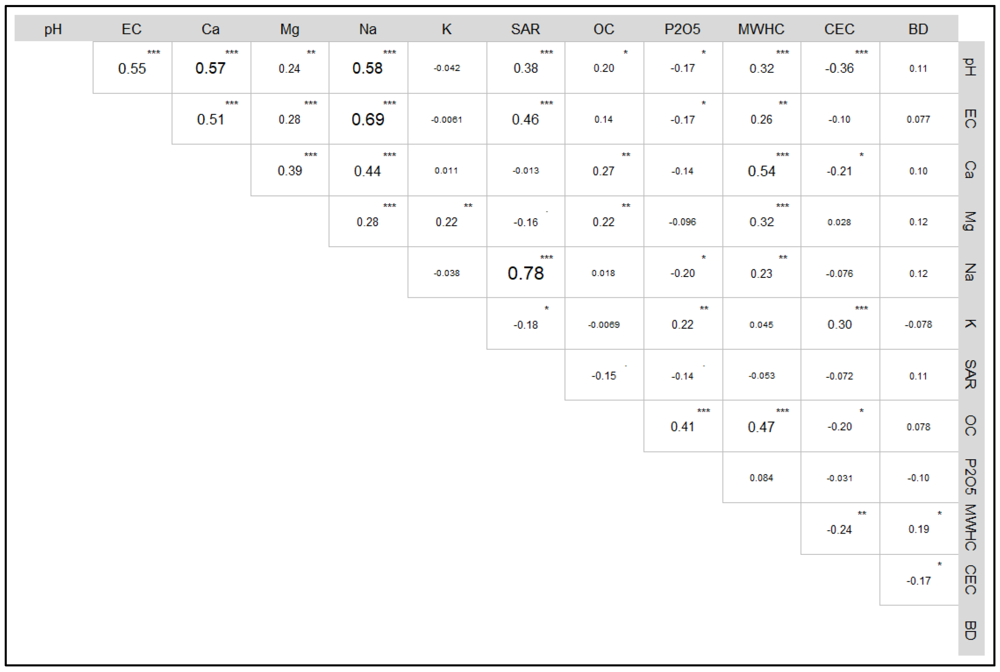
3.1. Descriptive Statistics of Soil Properties

Descriptive statistics of soil parameters are presented in

Table 3. Descriptive statistics of soil properties.

	pH	EC (dSm−1)	Ca	Mg	Na	K	SAR	OC (%)	Avl. P2O5 (kg ha−1)	MWHC (%)	CEC cmol/kg	BD (g cm−3)
			(meq/100 g)
Max	9.05	1.39	20.70	17.70	1.99	1.18	19.18	2.54	233.15	65.40	33.3	1.4
Min	4.46	0.06	0.80	0.40	0.03	0.04	0.36	0.15	2.09	17.60	22.9	1.33
Mean	6.90	0.36	8.18	4.82	0.36	0.21	2.83	0.97	62.08	41.55	25.83	1.36
Std Dev	0.96	0.24	4.35	3.06	0.33	0.15	2.39	0.52	58.06	7.37	16.07	1.38
CV (%)	13.90	65.77	53.27	63.45	89.48	72.89	84.42	53.48	93.52	17.73	6.22	1.01
Skewness	−0.46	1.65	0.58	1.17	2.42	2.79	3.66	0.69	1.19	−0.13	1.71	−0.19
Kurtosis	−0.47	3.38	−0.35	1.58	7.28	12.54	19.30	0.02	0.40	0.73	5.26	−0.07

pH—soil reaction; EC—electrical conductivity; Ca—exchangeable calcium; Mg—exchangeable magnesium; Na—exchangeable sodium; K—exchangeable potassium; SAR—sodium adsorption ratio; Avl. P₂O₅—available phosphorous; MWHC—maximum water holding capacity; CEC—cation exchange capacity; BD—bulk density; Std. Dev—standard deviation; CV—coefficient of variation.

. Except bulk density, all parameters exhibit high coefficients of variation, indicating significant variability. Values of pH ranged from acidic (4.46) to highly alkaline (9.05), with a mean of 6.90. Electrical conductivity ranged from 65 µS/m to 1390 µS/m, with a mean of 368 µS/m, suggesting the presence of problematic soils and considerable spatial heterogeneity in the study area. Similar findings were observed by Meena et al. [36] and Hegde et al. [44] in the Cauvery command area. The presence of problematic soils was evident, with high sodium adsorption ratio (SAR) values of 19.18 and positive skewness indicating potential areas with higher sodium content.

Exchangeable cation also exhibited significant variability with wide ranges: Ca: 0.8 to 20.7 meq/100 g, Mg: 0.4 to 17.7 meq/100 g, Na: 0.03 to 1.99 meq/100 g, and K: 0.04 to 1.18 meq/100 g. All the exchangeable cations had a positive skewness, indicating a more significant number of soil samples that showed higher values than the mean. Other important soil properties are soil organic carbon, available phosphorous, and cation exchange capacity; these also had higher CV with a range of 0.15 to 2.54%, 2.09 to 233.15 kg/ha, and 22.9 to 33.3 cmol/kg, respectively. Physical properties like bulk density and maximum water-holding capacity were also analyzed, and they varied from 1.33 to 1.40 g cm⁻³ and 17.6 to 65.40%, respectively.

Correlation analysis was also conducted to construct MDS and determine the link between various soil parameters. The largest negative correlations were found between pH and CEC (r = −0.36 ***) and MWHC and CEC (r = −0.24 **), while the highest positive correlations were found between Na and SAR (r = 0.78 ***), EC and Na (r = 0.69 ***), pH and Na (r = 0.58 ***), pH and Ca (r = 0.57 ***), and pH and EC (r = 0.55 ***) (Figure 3).

3.2. Principal Component Analysis and MDS

Principal component analysis was employed for the dataset to identify crucial indicators and to establish the MDS. The PCA is a widely accepted method for dimensionality reduction and indicator selection in MDS, as demonstrated in prior studies [12,47,51].

Table 4. Results of PCA for soil properties in the Cauvery command area.

	PC1	PC2	PC3	PC4	Communalities	Weightage
pH	0.417	0.033	0.168	0.141	0.223	0.084
EC	0.402	0.093	0.065	0.288	0.258	0.098
Ca	0.412	0.133	0.082	0.298	0.283	0.107
Mg	0.264	0.043	0.407	0.288
Na	0.406	0.339	0.015	0.211	0.324	0.123
K	0.022	0.124	0.533	0.331	0.409	0.155
SAR	0.293	0.418	0.211	0.381
OC	0.213	0.478	0.002	0.108	0.285	0.108
Avl_P2O5	0.025	0.397	0.128	0.572	0.501	0.19
MWHC	0.318	0.352	0.086	0.178
BD_cg/cm3	0.012	0.301	0.434	0.224
CEC_cmol/kg	0.165	0.255	0.505	0.078	0.353	0.134
Eigenvalues	3.2577	2.0704	1.4919	1.376
Proportion of variance	0.2715	0.1725	0.1243	0.1147
Cumulative variance	0.2715	0.444	0.5683	0.683

Underlined values are soil properties with the highest loading factors; bold factors are selected as MDS.

presents the PCA results, describing the data for 12 indicators.

The PCA yielded 12 principal components (PC), with the first 4 PCs showing eigenvalues greater than 1 (ranging from 1.37 to 3.25), and these PCs collectively contributed to 68.3% of the total variance. The first PC, covering 27.15% of the variance, featured pH as the key contributor, with the highest loading factor of 0.416. Additionally, EC (0.402), Na (0.406), and Ca (0.412) fell within a 90% threshold of the highest weighted factor. As the correlation values between EC, Ca, Na, and pH are below the threshold of 0.7 [59], these variables were believed to be suitable for inclusion in the MDS. The second PC, accounting for 17.25% of the total variance, highlighted organic carbon with a maximum loading factor of 0.47. At the same time, no other parameters met the threshold for inclusion in the MDS. The third PC, capturing 12.4% of the total variance, featured exchangeable potassium (K) with the highest loading factor of 0.53, followed by CEC (0.50). The correlation between K and CEC was <0.7; both the variables were retained for MDS. The fourth PC, contributing 11.47% to the cumulative variance of 68.3%, showcased available P₂O₅ with the highest loading factor of 0.57, with no other parameters meeting the 90% threshold for inclusion in the MDS. As a result, 8 soil parameters viz., pH, EC, Ca, Na, K, OC, Avl. P₂O_5, and CEC, were considered in the MDS out of the initial 12 soil parameters. The communality-based weightage assigned to these variables is presented in Table 4, ranging from 0.19 for available phosphate to 0.084 for pH.

3.3. Assessment of Soil Quality Index (SQI)

The identified soil quality indicators in the MDS were categorized into three classes: more is better (OC, CEC, Avl. P₂O₅, Ca, and K), less is better (Na), and optimum range (pH and EC). These indicators’ scores were calculated using linear and non-linear scoring methods (Equations (1)–(3)). Subsequently, the SQI was computed using the weights specified in Table 4 and the scores, resulting in SQI-LS (Equation (7)) and SQI-NLS (Equation (8)).

$$\begin{array}{c}\mathrm{S}\mathrm{Q}\mathrm{I}\text{-}\mathrm{L}\mathrm{S}=\left(\mathrm{L}\mathrm{S}\_\mathrm{p}\mathrm{H}\ast 0.084\right)+\left(\mathrm{L}\mathrm{S}\_\mathrm{E}\mathrm{C}\ast 0.097\right)+\left(\mathrm{L}\mathrm{S}\_\mathrm{C}\mathrm{a}\ast 0.10\right)+\left(\mathrm{L}\mathrm{S}\_\mathrm{N}\mathrm{a}\ast 0.122\right)+\left(\mathrm{L}\mathrm{S}\_\mathrm{K}\ast 0.155\right)\\ +\left(\mathrm{L}\mathrm{S}\_\mathrm{O}\mathrm{C}\ast 0.108\right)+\left(\mathrm{L}\mathrm{S}\_{\mathrm{P}}_2{\mathrm{O}}_5\ast 0.199\right)+(\mathrm{L}\mathrm{S}\_\mathrm{C}\mathrm{E}\mathrm{C}\ast 0.134)\end{array}$$

(7)

$$\begin{array}{c}\mathrm{S}\mathrm{Q}\mathrm{I}\text{-}\mathrm{N}\mathrm{L}\mathrm{S}=\left(\mathrm{N}\mathrm{L}\mathrm{S}\_\mathrm{p}\mathrm{H}\ast 0.084\right)+\left(\mathrm{N}\mathrm{L}\mathrm{S}\_\mathrm{E}\mathrm{C}\ast 0.097\right)+\left(\mathrm{N}\mathrm{L}\mathrm{S}\_\mathrm{C}\mathrm{a}\ast 0.10\right)+\left(\mathrm{N}\mathrm{L}\mathrm{S}\_\mathrm{N}\mathrm{a}\ast 0.122\right)+\left(\mathrm{N}\mathrm{L}\mathrm{S}\_\mathrm{K}\ast 0.155\right)\\ +\left(\mathrm{N}\mathrm{L}\mathrm{S}\_\mathrm{O}\mathrm{C}\ast 0.108\right)+\left(\mathrm{N}\mathrm{L}\mathrm{S}\_{\mathrm{P}}_2{\mathrm{O}}_5\ast 0.199\right)+(\mathrm{N}\mathrm{L}\mathrm{S}\_\mathrm{C}\mathrm{E}\mathrm{C}\ast 0.134)\end{array}$$

(8)

SQI-LS values ranged from 0.10 to 0.64, with a mean of 0.39, while SQI-NLS exhibited a broader range of 0.12 to 0.78, with a mean value of 0.48. The assessment of individual soil properties’ contributions to the SQI using linear scoring and non-linear scoring methods is shown in Figure 4. Under SQI-LS, sodium (Na) emerged as a significant contributor (constituting 25.69% of the SQI); conversely, potassium (K) exhibited a lower influence of 5.66%. In SQI-NLS, sodium was the primary influencer, but its impact was decreased to 15.85%, while potassium’s (K) influence increased to 13.28%.

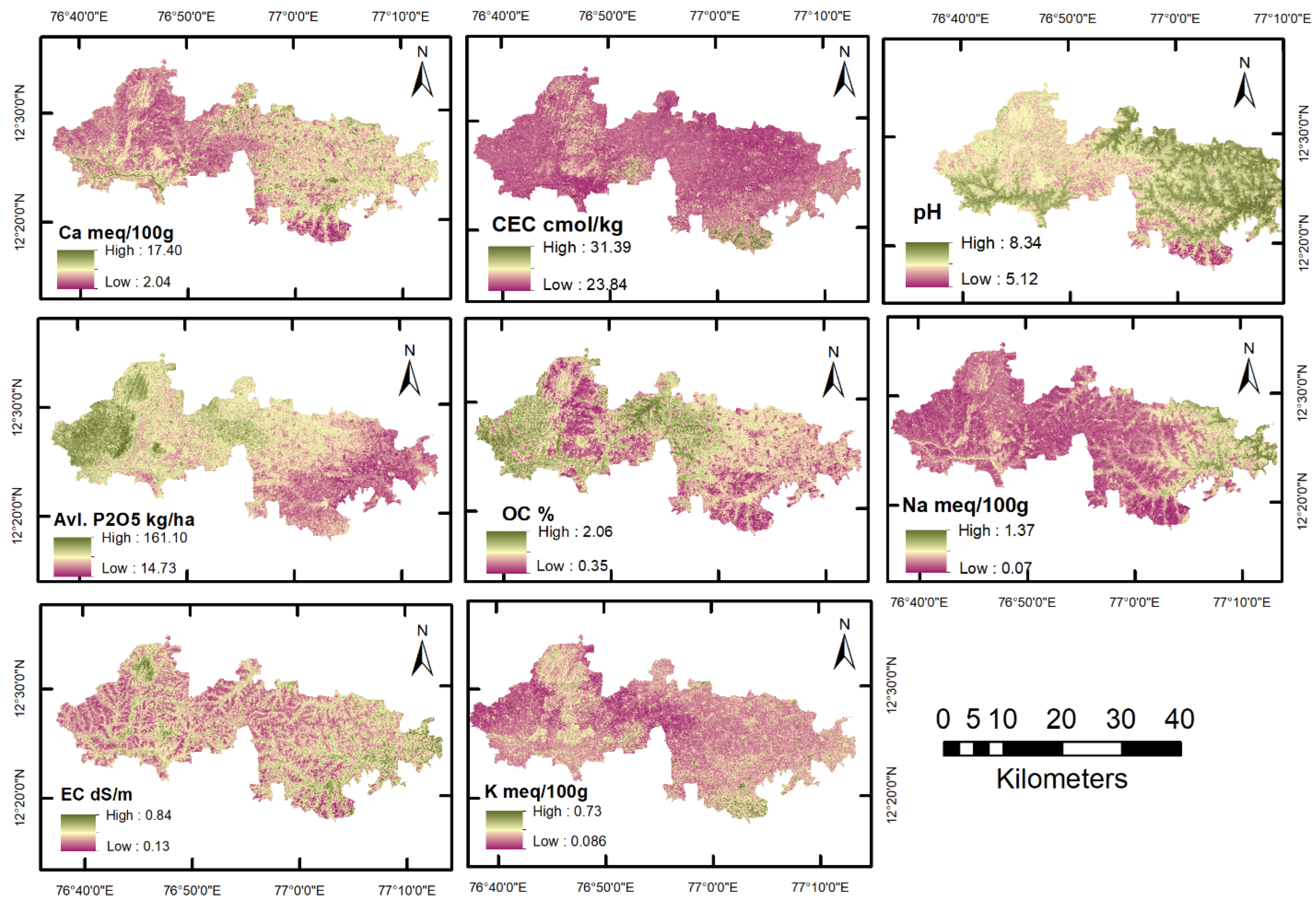
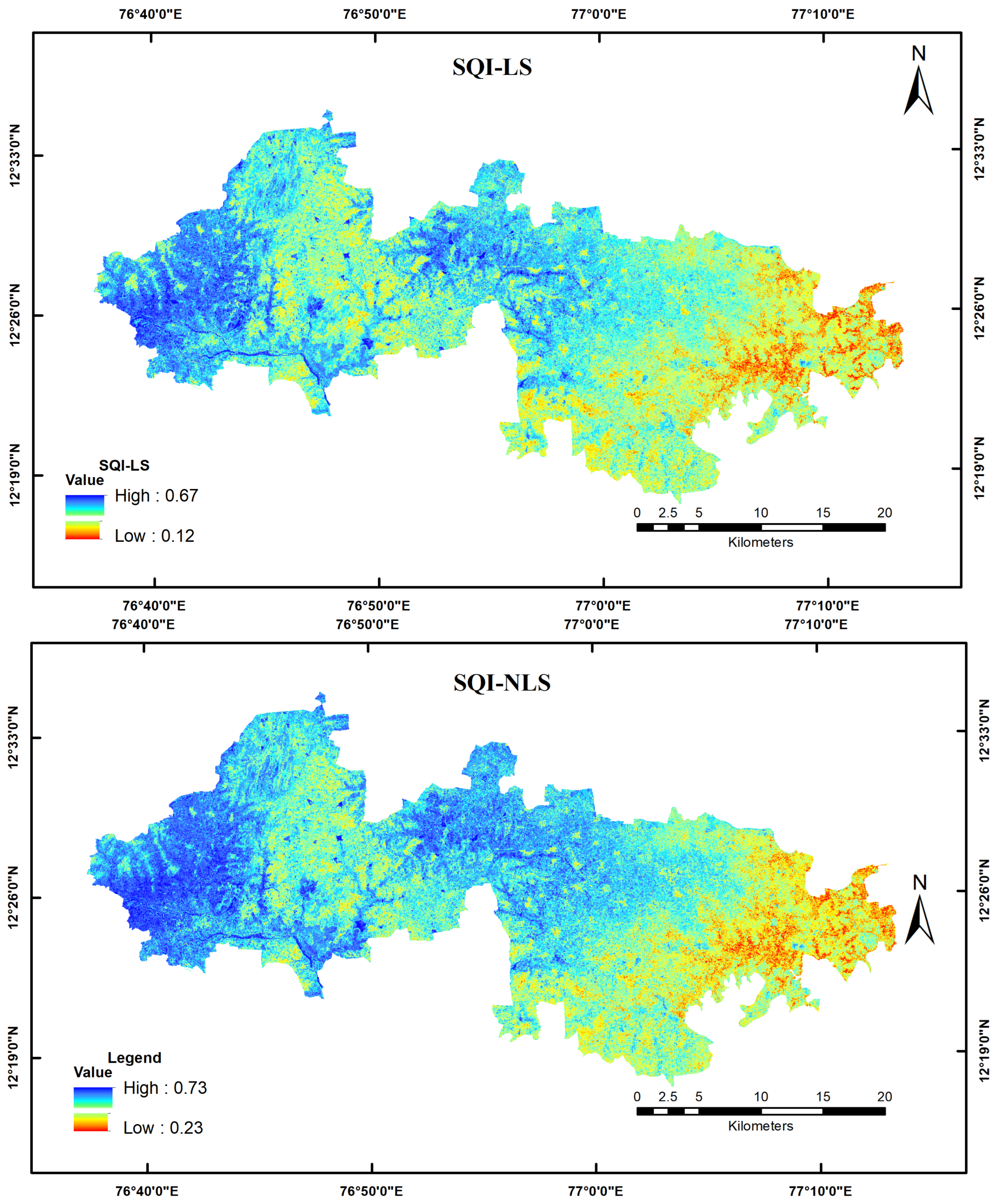
3.4. Spatial Assessment of SQI

Soil properties included in MDS were predicted for the study area using the tuned random forest model and environmental covariates (Table 1). The random forest model demonstrated strong predictive performance for most soil properties, except for potassium and available phosphorus (

Table 5. Performance of random forest for soil property prediction and model tuning parameters.

Soil Property	R2	Concordance	RMSE	Bias	ntree	mtry
pH	0.31	0.36	0.80	−0.03	280	8
EC	0.18	0.20	223	7.02	100	3
SOC	0.34	0.40	0.43	0.01	350	4
Ca	0.37	0.42	3.52	0.03	50	9
Na	0.24	0.32	0.27	0.01	48	9
CEC	0.33	0.36	12	0.18	500	9
K	0.09	0.05	0.14	0.01	1000	4
Avl. P2O5	0.07	0.09	59	3.88	500	9

). The highest coefficient of determination and Lin’s concordance correlation coefficient (CCC) were observed for calcium (Ca) predictions, with values of 0.37 and 0.42, respectively. This performance was achieved using 50 trees (ntree) and nine environmental variables at each node (mtry). Following Ca, soil organic carbon (SOC) exhibited better predictive capabilities, with an R² of 0.34 and CCC of 0.40. Similarly, cation exchange capacity (CEC) demonstrated promising performance, with an R² of 0.33 and CCC of 0.36. pH predictions also showed reasonably good results, with an R² of 0.31 and CCC of 0.36. Predictions for sodium (Na) and electrical conductivity (EC) yielded lower but still notable R² values of 0.24 and 0.18, respectively, with corresponding CCC values of 0.32 and 0.20.

Using the tuned random forest model, soil property maps of the study area were predicted and depicted in Figure 5. The predicted soil properties ranged from pH 5.12 to 8.34, EC 134 to 847 µS/m, OC 0.35 to 2.06%, Na 0.07 to 1.37 mEq/100 g, CEC 23.8 to 31.3 cmol/kg, Ca 2 to 17.4 mEq/100 g, K 0.08 to 0.73 mEq/100 g, and available phosphorous 14.7 to 161 Kg/ha.

Using the predicted soil property rasters (Figure 5) and the scoring functions (Equations (1)–(3)), along with the specified weights, spatial maps representing the SQI maps (Figure 6) for both the linear (SQI-LS) and non-linear (SQI-NLS) scoring approaches were generated. This was achieved by applying Equations (7) and (8), respectively. Non-linear (SQI-NLS) scoring approaches were obtained (Figure 6). Predicted SQI-LS values ranged from 0.12 to 0.67 with a mean of 0.47, and SQI-NLS values varied between 0.23 and 0.73 with a mean value of 0.56. Both soil quality maps show similar patterns of spatial variability. Western and central parts of the study area show higher SQI, and eastern parts show poorer quality soil.

The accuracy assessment of predicted SQI maps was performed using several metrics, including the R², LCC, RMSE, and bias. Two linear regression plots (Figure 7) were constructed to illustrate the relationships between estimated and predicted SQI values. The results indicate that the non-linear scoring method produced superior predictions, with a higher R² of 0.66 between predicted and observed SQI values. This method also exhibited low RMSE (0.08), bias (−0.05) values, and a high LCC of 0.66. Conversely, SQI maps established using linear scoring showed slightly lower values of R² (0.60) and LCC (0.65), along with higher RMSE (0.09) and bias (−0.06) values.

The soil quality assessment continued with the classification of developed SQI maps into five distinct quality grades following the thresholds provided in Table 2. The classified soil quality grade maps are depicted in Figure 8. The data in

Table 6. Area under various grades of soil quality index (ha).

Grade	SQI-LS	SQI-NLS
I (very high)	17,121 (18.82)	21,168 (23.27)
II (high)	26,058 (28.64)	26,130 (28.72)
III (moderate)	26,105 (28.69)	24,330 (26.74)
IV (low)	17,131 (18.83)	15,012 (16.50)
V (very low)	4545 (4.99)	4320 (4.74)

Values in parentheses are the percent of the total area.

further detail the area corresponding to each grade class in each type of SQI map.

More than 50% of the area fell into grades II and III on SQI maps created using LS and NLS, indicating that most of the study area’s soils have high-to-moderate soil quality. SQI-NLS had more area in grade I (23.27%) than SQI-LS (18.82%). Conversely, SQI-LS had more area in grade IV (18.83%) than SQI-NLS (16.5%), while in both scoring methods, the area under grade V was of a similar extent.

4. Discussion

4.1. PCA, Scoring, and SQI Assessment

The soil properties analyzed in this study show significant variability. The measurements for pH, EC, and Na suggest that the soils in the study area range from slightly acidic to alkaline. Similar findings were reported by Meena et al. [36] and Hegde et al. [44] in the Cauvery command area, where they have observed alkaline soils. This variability can be linked to the uneven topography [56] and the cultivation of water-intensive crops like paddy [57]. Additionally, the high levels of available phosphorus are likely due to the overuse of phosphate fertilizers, resulting in phosphorus buildup in the soils [58].

Correlation across soil parameters, along with amount of time and money required for thorough soil data collection and analysis underscores the need for development of MDS, which helps to reduce redundant data while maximizing relevant information [60].

Principal component analysis and correlation analysis was used for MDS development. Out of initial 12 parameters, pH, EC, Ca, Na, K, OC, available phosphorous, and CEC were considered in the MDS. MDS compiled by various researchers [13,16,23,47,50,51,61] for SQI assessment consistently featured a selection of similar fundamental soil properties. pH’s influence on nutrient availability [62,63], EC as a salinity proxy [64], and OC’s impact on various soil properties underscores their importance [65,66].

Soils characterized by extreme values, both higher and lower, in electrical conductivity (EC) and pH, alongside lower levels of organic carbon (OC), calcium (Ca), potassium (K), phosphorus (P₂O₅), and cation exchange capacity (CEC), accompanied by elevated sodium (Na) content, consistently exhibited lower scores and SQI. [15,28,50,67]. This observation was held for linear (SQI-LS) and non-linear (SQI-NLS) scoring methods. Notably, SQI-NLS demonstrated higher maximum and lower minimum values, indicating greater sensitivity than SQI-LS. SQI-NLS’s higher sensitivity index suggests its enhanced ability to differentiate among various soil quality scenarios. Nabiollahi et al. [51] also found the superiority of non-linear scoring for the sensitivity of the SQI.

The results of contribution of individual soil quality indicators for SQI reveal that sodium contributed the most, followed by electrical conductivity and available phosphorus (Figure 4), both of which exhibited extreme maximum and minimum values. On the other hand, the non-linear scoring method, which considers the mean values of indicators, showed relatively equal contributions from all indicators, with a slightly higher contribution from sodium (Na). This disparity in contribution patterns between the two scoring methods underscores the sensitivity of the scoring approach to the calculation methodology. Similar performance of a non-linear scoring method for SI was observed by Zornoza, et al. [52] in Mediterranean natural forests. Further, the multifaceted impact of electrical conductivity and sodium on SQI can be observed in the study, reflecting the intricate relationship between soil properties and plant health. EC, indicative of soil salinity, can have both positive and negative effects on soil fertility and plant growth. While moderate EC levels enhance nutrient availability, ion balance, and microbial activity [68], excessive salinity can detrimentally affect soil structure and plant health [69]. Similarly, sodium, though essential for maintaining osmotic balance [70] at moderate levels, when present in excess concentrations can lead to soil sodicity and poor drainage [71]. The present study’s scoring system, employing an “optimum is better” approach, appropriately accounts for these complexities, assigning higher scores to moderate EC and Na levels while penalizing high levels indicative of salinity and sodicity issues.

The findings suggest that the scoring method can influence the perceived importance of individual soil quality indicators in the overall assessment, emphasizing the need for careful consideration in selecting the scoring approach. The prevalence of sodic soils in the study area is primarily attributed to unregulated irrigation practices, fertilizer usage, and climatic conditions [36,44]. This has led to the dominance of exchangeable sodium as the primary cation in these soils, significantly impacting both soil quality and crop productivity; thus, exchangeable sodium emerged as the foremost determinant influencing the SQI. These findings are consistent with those of various studies [15,51], where assessments of SQI in salt-affected soils similarly emphasized the substantial role of exchangeable sodium percentage.

4.2. Spatial Assessment of Soil Properties and Soil Quality

There are two approaches to calculating and mapping the SQI: (i) calculating the SQI for each sample point first and then spatializing the SQI, and (ii) spatializing individual soil properties first and then calculating the SQI. In the present study, we chose the latter approach for several reasons. Firstly, this method allows for a detailed examination of the spatial variability and distribution of each soil property across the study area [72]. Secondly, transforming soil properties into dimensionless units before SQI calculation standardizes the data, ensuring that each property contributes equally to the overall index and mitigating the risk of one highly variable property disproportionately influencing the SQI [47].

Furthermore, scoring functions and weights were applied to each soil indicator, reflecting their unique contributions to overall soil quality. These functions can be adjusted based on optimal ranges for each parameter, enhancing the accuracy and relevance of the SQI maps. However, direct prediction of SQI without considering these customized scoring functions and weights could lead to inaccuracies, as it would overlook the distinct contributions and significance of each soil property in determining overall soil quality [49]. Therefore, spatializing individual soil properties before SQI calculation allows for a more accurate assessment of soil quality across the study.

Following the second approach, a random forest model was employed to predict eight soil properties identified as the MDS. Model performance was evaluated using the coefficient of determination and CCC, with values ranging between 0.07 to 0.37 and 0.05 to 0.42, respectively, indicating varying levels of accuracy in the predictions. Notably, potassium and phosphorus exhibited lower predictive accuracy, attributed to the region’s wide variability in crop management practices, nutrient application, and vegetation cover [73,74,75,76]. Despite their lower accuracy, the inclusion of potassium and phosphorus in the SQI assessment is justified by their essential roles in plant growth and soil fertility [77]. These nutrients play critical roles in various physiological processes within plants, directly influencing crop productivity and overall soil health [77]. Furthermore, while their predictive accuracy may be limited, their presence in the SQI offers valuable diagnostic information, guiding targeted soil management interventions to optimize conditions for crop production.

Predicted soil property maps reveal significant variability across the study area, particularly evident in the eastern and southwestern regions. Lower elevation in these areas may have led to leaching of salts from higher elevated central parts, contributing to increased pH and electrical conductivity. Park et al. [70] found similar reasons for increased salinity in paddy-growing soils of southwestern coastal areas of South Korea. The leaching process was further evident with higher concentrations of exchangeable cations (Ca, Na, and K) in these regions, and elevated concentrations of these ions will increase pH and EC [36,44]. Conversely, the distribution of soil organic carbon content varied across the study area, with central and western parts having higher organic carbon content. The reason for higher soil organic carbon contents could be attributed to addition of paddy stubbles and sugarcane trash, as paddy and sugarcane are the principal crops of command area [78,79]. Moreover, available phosphorous was higher in western parts while eastern parts had the lowest contents. Compared to all other soil indicators, the minor spatial variability was associated with cation exchange capacity, possibly due to dominance of monomineralic parent material [80].

Further, SQI maps were generated using linear and non-linear scoring methods based on predicted soil indicators shows, and eastern areas with lower elevation exhibited poorer soil quality than the western parts. This observation aligns with findings from Nabhiollahi et al. [81], who assessed the impact of slope and elevation on SQI, concluding that SQI tends to decrease with lower elevations. The generated SQI maps confirm this trend, indicating poorer soil quality in the eastern regions and higher SQI values in the western areas. When evaluating the accuracy of these maps, the non-linear scoring method outperformed the linear method. The non-linear approach, which uses mean values of soil properties, demonstrated higher accuracy due to smaller differences between actual and predicted mean values. In contrast, the linear scoring method, which takes into account the maximum and minimum values of soil properties, showed greater variation between actual and predicted values. The performance of scoring methods varied across different studies [14,19,51,61,82], suggesting that the choice of scoring method depends on specific study area and the soil parameters included in the MDS.

The SQI maps (Figure 7) were classified into five grades to prioritize management strategies. The SQI-LS and SQI-NLS classified maps (Figure 8) show that over 50% of the soils in the study area have high-to-moderate soil quality and may not require dedicated management practices. However, more than 20% of the soils belong to the low-to-very-low category of soil quality, concentrated in the eastern parts of the study area, requiring immediate and dedicated management strategies.

5. Conclusions

In this study, two scoring methods were used to assess soil quality in the Cauvery command area. PCA was used to identify indicators to include in the MDS; this method reduces the multicollinearity effect of highly correlated soil properties and displays the information in other selected properties. Eight soil parameters—pH, EC, Ca, Na, K, OC, available P₂O₅, and CEC—were identified as critical soil quality indicators and included in the MDS.

The RF model integrated with various environmental covariates effectively predicted the MDS soil properties. The SQI spatial maps developed from the predicted soil properties highlight the intricate spatial variability of soil quality across the region. With higher R² and LCC, the non-linear scoring method was found to be better at predicting SQI than the linear scoring method. The SQI maps reveal high spatial variability with more than 40 percent of soils classified as moderate-to-low index. The soils with low SQI were distributed in eastern parts, whereas western parts exhibited high-to-very-high soil quality. Results also reveal electrical conductivity and sodium content have the highest influence on soil quality, emphasizing the need for targeted soil management practices, particularly in the eastern regions. The findings underscore the importance of soil quality assessment for informed decision-making related to cultivation patterns, irrigation management, and overall soil health enhancement.

References

1. Sánchez-Navarro, A.; Gil-Vázquez, J.M.; Delgado-Iniesta, M.J.; Marín-Sanleandro, P.; Blanco-Bernardeau, A.; Ortiz-Silla, R. Establishing an Index and Identification of Limiting Parameters for Characterizing Soil Quality in Mediterranean Ecosystems. Catena 2015, 131, 35–45. [Google Scholar] [CrossRef]
2. Zhu, W.; Pan, Y.; He, H.; Wang, L.; Mou, M.; Liu, J. A Changing-Weight Filter Method for Reconstructing a High-Quality NDVI Time Series to Preserve the Integrity of Vegetation Phenology. IEEE Trans. Geosci. Remote Sens. 2012, 50, 1085–1094. [Google Scholar] [CrossRef]
3. Weis, T. The Accelerating Biophysical Contradictions of Industrial Capitalist Agriculture. J. Agrar. Change 2010, 10, 315–341. [Google Scholar] [CrossRef]
4. Power, A.G. Ecosystem Services and Agriculture: Tradeoffs and Synergies. Philos. Trans. R. Soc. B Biol. Sci. 2010, 365, 2959–2971. [Google Scholar] [CrossRef] [PubMed]
5. Lorenz, K.; Lal, R. Biochar Application to Soil for Climate Change Mitigation by Soil Organic Carbon Sequestration. Wiley Online Libr. 2014, 177, 651–670. [Google Scholar] [CrossRef]
6. Singh, D.K.; Jaiswal, C.S.; Reddy, K.S.; Singh, R.M.; Bhandarkar, D.M. Optimal Cropping Pattern in a Canal Command Area. Agric. Water Manag. 2001, 50, 1–8. [Google Scholar] [CrossRef]
7. Yi, J.; Li, H.; Zhao, Y.; Shao, M.; Zhang, H.; Liu, M. Assessing Soil Water Balance to Optimize Irrigation Schedules of Flood-Irrigated Maize Fields with Different Cultivation Histories in the Arid Region. Agric. Water Manag. 2022, 265, 107543. [Google Scholar] [CrossRef]
8. Kalambukattu, J.G.; Johns, B.; Kumar, S.; Raj, A.D.; Ellur, R. Temporal Remote Sensing Based Soil Salinity Mapping in Indo-Gangetic Plain Employing Machine-Learning Techniques. Proc. Indian Natl. Sci. Acad. 2023, 89, 290–305. [Google Scholar] [CrossRef]
9. Das, A.; Lal, R.; Patel, D.P.; Idapuganti, R.G.; Layek, J.; Ngachan, S.V.; Ghosh, P.K.; Bordoloi, J.; Kumar, M. Effects of Tillage and Biomass on Soil Quality and Productivity of Lowland Rice Cultivation by Small Scale Farmers in North Eastern India. Soil Tillage Res. 2014, 143, 50–58. [Google Scholar] [CrossRef]
10. Zhang, T.; Li, H.; Yan, T.; Shaheen, S.M.; Niu, Y.; Xie, S.; Zhang, Y.; Abdelrahman, H.; Ali, E.F.; Bolan, N.S.; et al. Organic Matter Stabilization and Phosphorus Activation during Vegetable Waste Composting: Multivariate and Multiscale Investigation. Sci. Total Environ. 2023, 891, 164608. [Google Scholar] [CrossRef]
11. He, M.Y.; Dong, J.B.; Jin, Z.; Liu, C.Y.; Xiao, J.; Zhang, F.; Sun, H.; Zhao, Z.Q.; Gou, L.F.; Liu, W.G.; et al. Pedogenic Processes in Loess-Paleosol Sediments: Clues from Li Isotopes of Leachate in Luochuan Loess. Geochim. Cosmochim. Acta 2021, 299, 151–162. [Google Scholar] [CrossRef]
12. Andrews, S.S.; Mitchell, J.P.; Mancinelli, R.; Karlen, D.L.; Hartz, T.K.; Horwath, W.R.; Pettygrove, G.S.; Scow, K.M.; Munk, D.S. On-Farm Assessment of Soil Quality in California’s Central Valley. Agron. J. 2002, 94, 12–23. [Google Scholar] [CrossRef]
13. Adelana, A.; Aduramigba-Modupe, V.; Oke, A.; Are, K.; Ojo, O.; Adeyolanu, O. Soil Quality Assessment under Different Long-Term Rice-Based Cropping Systems in a Tropical Dry Savanna Ecology of Northern Nigeria. Acta Ecol. Sin. 2022, 42, 312–321. [Google Scholar] [CrossRef]
14. Maleki, S.; Zeraatpisheh, M.; Karimi, A.; Sareban, G.; Wang, L. Assessing Variation of Soil Quality in Agroecosystem in an Arid Environment Using Digital Soil Mapping. Agronomy 2022, 12, 578. [Google Scholar] [CrossRef]
15. Mahajan, G.; Das, B.; Morajkar, S.; Desai, A.; Murgaokar, D.; Kulkarni, R.; Sale, R.; Patel, K. Soil Quality Assessment of Coastal Salt-Affected Acid Soils of India. Environ. Sci. Pollut. Res. 2020, 27, 26221–26238. [Google Scholar] [CrossRef]
16. Rezaee, L.; Moosavi, A.A.; Davatgar, N.; Sepaskhah, A.R. Soil Quality Indices of Paddy Soils in Guilan Province of Northern Iran: Spatial Variability and Their Influential Parameters. Ecol. Indic. 2020, 117, 106566. [Google Scholar] [CrossRef]
17. Cooper, P.J.M.; Dimes, J.; Rao, K.P.C.; Shapiro, B.; Shiferaw, B.; Twomlow, S. Coping Better with Current Climatic Variability in the Rain-Fed Farming Systems of Sub-Saharan Africa: An Essential First Step in Adapting to Future Climate Change? Agric. Ecosyst. Environ. 2008, 126, 24–35. [Google Scholar] [CrossRef]
18. Shiferaw, B.A.; Okello, J.; Reddy, R.V. Adoption and Adaptation of Natural Resource Management Innovations in Smallholder Agriculture: Reflections on Key Lessons and Best Practices. Environ. Dev. Sustain. 2009, 11, 601–619. [Google Scholar] [CrossRef]
19. Nabiollahi, K.; Taghizadeh-Mehrjardi, R.; Eskandari, S. Assessing and Monitoring the Soil Quality of Forested and Agricultural Areas Using Soil-Quality Indices and Digital Soil-Mapping in a Semi-Arid Environment. Arch. Agron. Soil Sci. 2017, 64, 696–707. [Google Scholar] [CrossRef]
20. Zhang, T.; Song, B.; Han, G.; Zhao, H.; Hu, Q.; Zhao, Y.; Liu, H. Effects of Coastal Wetland Reclamation on Soil Organic Carbon, Total Nitrogen, and Total Phosphorus in China: A Meta-Analysis. Land Degrad. Dev. 2023, 34, 3340–3349. [Google Scholar] [CrossRef]
21. McBratney, A.B.; Mendonça Santos, M.L.; Minasny, B. On Digital Soil Mapping. Geoderma 2003, 117, 3–52. [Google Scholar] [CrossRef]
22. Parent, E.J.; Parent, S.É.; Parent, L.E. Determining Soil Particle-Size Distribution from Infrared Spectra Using Machine Learning Predictions: Methodology and Modeling. PLoS ONE 2021, 16, e0233242. [Google Scholar] [CrossRef] [PubMed]
23. Choudhury, B.U.; Mandal, S. Indexing Soil Properties through Constructing Minimum Datasets for Soil Quality Assessment of Surface and Profile Soils of Intermontane Valley (Barak, North East India). Ecol. Indic. 2021, 123, 107369. [Google Scholar] [CrossRef]
24. Rosemary, F.; Vitharana, U.W.A.; Indraratne, S.P.; Weerasooriya, R.; Mishra, U. Exploring the Spatial Variability of Soil Properties in an Alfisol Soil Catena. Catena 2017, 150, 53–61. [Google Scholar] [CrossRef]
25. Dharumarajan, S.; Kalaiselvi, B.; Suputhra, A.; Lalitha, M.; Vasundhara, R.; Kumar, K.A.; Nair, K.M.; Hegde, R.; Singh, S.K.; Lagacherie, P. Digital Soil Mapping of Soil Organic Carbon Stocks in Western Ghats, South India. Geoderma Reg. 2021, 25, e00387. [Google Scholar] [CrossRef]
26. Mitran, T.; Mishra, U.; Lal, R.; Ravisankar, T.; Sreenivas, K. Spatial Distribution of Soil Carbon Stocks in a Semi-Arid Region of India. Geoderma Reg. 2018, 15, e00192. [Google Scholar] [CrossRef]
27. Peng, Y.; Zhao, L.; Hu, Y.; Wang, G.; Wang, L.; Liu, Z. Prediction of Soil Nutrient Contents Using Visible and Near-Infrared Reflectance Spectroscopy. ISPRS Int. J. Geo-Inf. 2019, 8, 437. [Google Scholar] [CrossRef]
28. Mamehpour, N.; Rezapour, S.; Ghaemian, N. Quantitative Assessment of Soil Quality Indices for Urban Croplands in a Calcareous. Geoderma 2021, 382, 114781. [Google Scholar] [CrossRef]
29. Astle, W.L.; Webster, R.; Lawrance, C.J. Land Classification for Management Planning in the Luangwa Valley of Zambia. J. Appl. Ecol. 1969, 6, 143. [Google Scholar] [CrossRef]
30. Jiang, H.; Rusuli, Y.; Amuti, T.; He, Q. Quantitative Assessment of Soil Salinity Using Multi-Source Remote Sensing Data Based on the Support Vector Machine and Artificial Neural Network. Int. J. Remote Sens. 2019, 40, 284–306. [Google Scholar] [CrossRef]
31. Tiwari, S.K.; Saha, S.K.; Kumar, S. Prediction Modeling and Mapping of Soil Carbon Content Using Artificial Neural Network, Hyperspectral Satellite Data and Field Spectroscopy. Adv. Remote Sens. 2015, 04, 63–72. [Google Scholar] [CrossRef]
32. Were, K.; Bui, D.T.; Dick, Ø.B.; Singh, B.R. A Comparative Assessment of Support Vector Regression, Artificial Neural Networks, and Random Forests for Predicting and Mapping Soil Organic Carbon Stocks across an Afromontane Landscape. Ecol. Indic. 2015, 52, 394–403. [Google Scholar] [CrossRef]
33. Hogland, J.; Billor, N.; Anderson, N. Comparison of Standard Maximum Likelihood Classification and Polytomous Logistic Regression Used in Remote Sensing. Eur. J. Remote Sens. 2013, 46, 623–640. [Google Scholar] [CrossRef]
34. Lenka, N.K.; Meena, B.P.; Lal, R.; Khandagle, A.; Lenka, S.; Shirale, A.O. Comparing Four Indexing Approaches to Define Soil Quality in an Intensively Cropped Region of Northern India. Front. Environ. Sci. 2022, 10, 865473. [Google Scholar] [CrossRef]
35. Lal, R. World reference base for soil resources. In Encyclopedia of Soil Science—Two-Volume Set; CRC Press: Boca Raton, FL, USA, 2005; pp. 1918–1923. [Google Scholar] [CrossRef]
36. Meena, R.S.; Natarajan, A.; Hegde, R.; Dhanorkar, B.A.; Koyal, A.; Naidu, L.G.K. Characterization and Classification of Upland Soils of Chikkarsinkere Hobli, Maddur Taluk, Mandya District of Karnataka. Agropedology 2014, 25, 154–160. [Google Scholar]
37. Jackson, M.L. Aluminum Bonding in Soils: A Unifying Principle in Soil Science. Soil Sci. Soc. Am. J. 1963, 27, 1–10. [Google Scholar] [CrossRef]
38. Pansu, M.; Gautheyrou, J. Exchangeable cations. In Handbook of Soil Analysis; Springer: Berlin/Heidelberg, Germany, 2006; pp. 667–676. [Google Scholar] [CrossRef]
39. Olsen, S.R.; Watanabe, F.S. A Method to Determine a Phosphorus Adsorption Maximum of Soils as Measured by the Langmuir Isotherm. Soil Sci. Soc. Am. J. 1957, 21, 144–149. [Google Scholar] [CrossRef]
40. Walkley, A. A Critical Examination of A Rapid Method For Determining Organic Carbon In Soils—Effect of Variations In Digestion Conditions and of Inorganic Soil Constituents. Soil Sci. 1947, 64, 251–264. [Google Scholar] [CrossRef]
41. Karlen, D.L.; Mausbach, M.J.; Doran, J.W.; Cline, R.G.; Harris, R.F.; Schuman, G.E. Soil Quality: A Concept, Definition, and Framework for Evaluation (A Guest Editorial). Soil Sci. Soc. Am. J. 1997, 61, 4–10. [Google Scholar] [CrossRef]
42. Carter, M.R. Soil Quality for Sustainable Land Management. Agron. J. 2002, 94, 38–47. [Google Scholar] [CrossRef]
43. Kibblewhite, M.G.; Ritz, K.; Swift, M.J. Soil Health in Agricultural Systems. Philos. Trans. R. Soc. B Biol. Sci. 2008, 363, 685–701. [Google Scholar] [CrossRef]
44. Hegde, R.; Natarajan, A.; Meena, R.S.; Niranjana, K.V.; Thayalan, S.; Singh, S.K. Status of Soil Degradation in an Irrigated Command Area in Chikkarasinakere Hobli, Mandya District, Karnataka. Curr. Sci. 2015, 108, 1501–1511. [Google Scholar]
45. Wander, M.M.; Bollero, G.A. Soil Quality Assessment of Tillage Impacts in Illinois. Soil Sci. Soc. Am. J. 1999, 63, 961–971. [Google Scholar] [CrossRef]
46. Govaerts, B.; Sayre, K.D.; Deckers, J. A Minimum Data Set for Soil Quality Assessment of Wheat and Maize Cropping in the Highlands of Mexico. Soil Tillage Res. 2006, 87, 163–174. [Google Scholar] [CrossRef]
47. Andrews, S.S.; Karlen, D.L.; Cambardella, C.A. The Soil Management Assessment Framework. Soil Sci. Soc. Am. J. 2004, 68, 1945–1962. [Google Scholar] [CrossRef]
48. Lamichhane, S.; Kumar, L.; Wilson, B. Digital Soil Mapping Algorithms and Covariates for Soil Organic Carbon Mapping and Their Implications: A Review. Geoderma 2019, 352, 395–413. [Google Scholar] [CrossRef]
49. Mukherjee, A.; Lal, R. Comparison of Soil Quality Index Using Three Methods. PLoS ONE 2014, 9, e105981. [Google Scholar] [CrossRef] [PubMed]
50. Biswas, S.; Hazra, G.C.; Purakayastha, T.J.; Saha, N.; Mitran, T.; Singha Roy, S.; Basak, N.; Mandal, B. Establishment of Critical Limits of Indicators and Indices of Soil Quality in Rice-Rice Cropping Systems under Different Soil Orders. Geoderma 2017, 292, 34–48. [Google Scholar] [CrossRef]
51. Nabiollahi, K.; Taghizadeh-Mehrjardi, R.; Kerry, R.; Moradian, S. Assessment of Soil Quality Indices for Salt-Affected Agricultural Land in Kurdistan Province, Iran. Ecol. Indic. 2017, 83, 482–494. [Google Scholar] [CrossRef]
52. Zornoza, R.; Mataix-Solera, J.; Guerrero, C.; Arcenegui, V.; Mataix-Beneyto, J.; Gómez, I. Validating the Effectiveness and Sensitivity of Two Soil Quality Indices Based on Natural Forest Soils under Mediterranean Conditions. Soil Biol. Biochem. 2008, 40, 2079–2087. [Google Scholar] [CrossRef]
53. Dharumarajan, S.; Hegde, R.; Singh, S.K. Spatial Prediction of Major Soil Properties Using Random Forest Techniques—A Case Study in Semi-Arid Tropics of South India. Geoderma Reg. 2017, 10, 154–162. [Google Scholar] [CrossRef]
54. Khanal, S.; Fulton, J.; Klopfenstein, A.; Douridas, N. Integration of High Resolution Remotely Sensed Data and Machine Learning Techniques for Spatial Prediction of Soil Properties and Corn Yield. Comput. Electron. Agric. 2018, 153, 213–225. [Google Scholar] [CrossRef]
55. Guo, L.; Linderman, M.; Shi, T.; Chen, Y.; Duan, L.; Zhang, H. Exploring the Sensitivity of Sampling Density in Digital Mapping of Soil Organic Carbon and Its Application in Soil Sampling. Remote Sens. 2018, 10, 888. [Google Scholar] [CrossRef]
56. Zeraatpisheh, M.; Ayoubi, S.; Jafari, A.; Tajik, S.; Finke, P. Digital Mapping of Soil Properties Using Multiple Machine Learning in a Semi-Arid Region, Central Iran. Geoderma 2019, 338, 445–452. [Google Scholar] [CrossRef]
57. Sreenivas, K.; Dadhwal, V.K.; Kumar, S.; Harsha, G.S.; Mitran, T.; Sujatha, G.; Rama, G.J.; Fyzee, M.A.; Ravisankar, T. Digital Mapping of Soil Organic and Inorganic Carbon Status in India. Geoderma 2016, 269, 160–173. [Google Scholar] [CrossRef]
58. Fick, S.E.; Hijmans, R.J. WorldClim 2: New 1-Km Spatial Resolution Climate Surfaces for Global Land Areas. Int. J. Climatol. 2017, 37, 4302–4315. [Google Scholar] [CrossRef]
59. Li, J.; Heap, A.D. Spatial Interpolation Methods Applied in the Environmental Sciences: A Review. Environ. Model. Softw. 2014, 53, 173–189. [Google Scholar] [CrossRef]
60. Carter, M.R.; Gregorich, E.G.; Anderson, D.W.; Doran, J.W.; Janzen, H.H.; Pierce, F.J. Concepts of Soil Quality and Their Significance. Dev. Soil Sci. 1997, 25, 1–19. [Google Scholar] [CrossRef]
61. Sheidai Karkaj, E.; Sepehry, A.; Barani, H.; Motamedi, J.; Shahbazi, F. Establishing a Suitable Soil Quality Index for Semi-Arid Rangeland Ecosystems in Northwest of Iran. J. Soil Sci. Plant Nutr. 2019, 19, 648–658. [Google Scholar] [CrossRef]
62. Sims, J.T. Soil PH Effects on the Distribution and Plant Availability of Manganese, Copper, and Zinc. Soil Sci. Soc. Am. J. 1986, 50, 367–373. [Google Scholar] [CrossRef]
63. Weaver, S.E.; Hamill, A.S. Effects of Soil PH on Competitive Ability and Leaf Nutrient Content of Corn (Zea Mays L.) and Three Weed Species. Weed Sci. 1985, 33, 447–451. [Google Scholar] [CrossRef]
64. Rhoades, J.D.; Manteghi, N.A.; Shouse, P.J.; Alves, W.J. Soil Electrical Conductivity and Soil Salinity: New Formulations and Calibrations. Soil Sci. Soc. Am. J. 1989, 53, 433–439. [Google Scholar] [CrossRef]
65. Fan, Y.; Zhang, Y.; Kalkhajeh, Y.K.; Hu, W.; Tian, K.; Yu, D.; Huang, B. Effective Indicators and Drivers of Soil Organic Matter in Intensive Orchard Production Systems. Soil Tillage Res. 2024, 238, 105999. [Google Scholar] [CrossRef]
66. Dexter, A.R.; Richard, G.; Arrouays, D.; Czyz, E.A.; Jolivet, C.; Duval, O. Complexed Organic Matter Controls Soil Physical Properties. Geoderma 2008, 144, 620–627. [Google Scholar] [CrossRef]
67. Hemmati, S.; Yaghmaeian, N.; Farhangi, M.B.; Sabouri, A. Soil Quality Assessment of Paddy Fields (in Northern Iran) with Different Productivities: Establishing the Critical Limits of Minimum Data Set Indicators. Environ. Sci. Pollut. Res. 2023, 30, 10286–10296. [Google Scholar] [CrossRef] [PubMed]
68. Smith, J.L.; Doran, J.W. Measurement and Use of PH and Electrical Conductivity for Soil Quality Analysis. Methods Assess. Soil Qual. 2015, 169–185. [Google Scholar] [CrossRef]
69. Ismayilov, A.I.; Mamedov, A.I.; Fujimaki, H.; Tsunekawa, A.; Levy, G.J. Soil Salinity Type Effects on the Relationship between the Electrical Conductivity and Salt Content for 1:5 Soil-to-Water Extract. Sustainability 2021, 13, 3395. [Google Scholar] [CrossRef]
70. Subbarao, G.V.; Ito, O.; Berry, W.L.; Wheeler, R.M. Sodium—A Functional Plant Nutrient. Crit. Rev. Plant Sci. 2003, 22, 391–416. [Google Scholar] [CrossRef]
71. Rengasamy, P.; Olsson, K.A. Sodicity and Soil Structure. Soil Res. 1991, 29, 935–952. [Google Scholar] [CrossRef]
72. Naimi, S.; Ayoubi, S.; Demattê, J.A.M.; Zeraatpisheh, M.; Amorim, M.T.A.; Mello, F.A.d.O. Spatial Prediction of Soil Surface Properties in an Arid Region Using Synthetic Soil Image and Machine Learning. Geocarto Int. 2022, 37, 8230–8253. [Google Scholar] [CrossRef]
73. Meroni, M.; Rossini, M.; Guanter, L.; Alonso, L.; Rascher, U.; Colombo, R.; Moreno, J. Remote Sensing of Environment Remote Sensing of Solar-Induced Chlorophyll Fl Uorescence: Review of Methods and Applications. Remote Sens. Environ. 2009, 113, 2037–2051. [Google Scholar] [CrossRef]
74. Nawar, S.; Corstanje, R.; Halcro, G.; Mulla, D.; Mouazen, A.M. Delineation of Soil Management Zones for Variable-Rate Fertilization: A Review, 1st ed.; Elsevier: Amsterdam, The Netherlands, 2017; Volume 143. [Google Scholar]
75. Tekin, A.B. Variable Rate Fertilizer Application in Turkish Wheat Agriculture: Economic Assessment. Afr. J. Agric.Res. 2010, 5, 647–652. [Google Scholar] [CrossRef]
76. Rajath, E.; Anush Kumar, K.; Setia, R.; Taneja, S.; Galohda, A.; Ansari, J.; Gupta, S.K.; Nigam, R.; Pateriya, B. Remote and Proximal Sensing for Optimising Input Use Efficiency for Sustainable Agriculture. Input Use Effic. Food Environ. Secur. 2022, 513–540. [Google Scholar] [CrossRef]
77. Wang, Y.; Chen, Y.F.; Wu, W.H. Potassium and Phosphorus Transport and Signaling in Plants. J. Integr. Plant Biol. 2021, 63, 34–52. [Google Scholar] [CrossRef] [PubMed]
78. Surendran, U.; Ramesh, V.; Jayakumar, M.; Marimuthu, S.; Sridevi, G. Improved Sugarcane Productivity with Tillage and Trash Management Practices in Semi Arid Tropical Agro Ecosystem in India. Soil Tillage Res. 2016, 158, 10–21. [Google Scholar] [CrossRef]
79. Yadav, R.L.; Prasad, S.R.; Singh, R.; Srivastava, V.K. Recycling Sugarcane Trash to Conserve Soil Organic Carbon for Sustaining Yields of Successive Ratoon Crops in Sugarcane. Bioresour. Technol. 1994, 49, 231–235. [Google Scholar] [CrossRef]
80. Ketterings, Q.M.; Gami, S.K.; Mathur, R.R.; Woods, M. A Simple Method for Estimating Effective Cation Exchange Capacity, Cation Saturation Ratios, and Sulfur across a Wide Range of Soils. Soil Sci. 2014, 179, 230–236. [Google Scholar] [CrossRef]
81. Nabiollahi, K.; Golmohamadi, F.; Taghizadeh-Mehrjardi, R.; Kerry, R.; Davari, M. Assessing the Effects of Slope Gradient and Land Use Change on Soil Quality Degradation through Digital Mapping of Soil Quality Indices and Soil Loss Rate. Geoderma 2018, 318, 16–28. [Google Scholar] [CrossRef]
82. Lagacherie, P.; Arrouays, D.; Bourennane, H.; Gomez, C.; Nkuba-Kasanda, L. Analysing the Impact of Soil Spatial Sampling on the Performances of Digital Soil Mapping Models and Their Evaluation: A Numerical Experiment on Quantile Random Forest Using Clay Contents Obtained from Vis-NIR-SWIR Hyperspectral Imagery. Geoderma 2020, 375, 114503. [Google Scholar] [CrossRef]
Figure 1. Location map of the study.
Land 13 00970 g001
Figure 2. Flowchart of the methodology followed in this for the study.
Land 13 00970 g002
Figure 3. Correlation between soil properties (p-values 0.001-***, 0.01-**, 0.05-*).
Land 13 00970 g003
Figure 4. Radar chart showing the contribution of different soil properties to SQI.
Land 13 00970 g004
Figure 5. Maps of predicted soil properties.
Land 13 00970 g005
Figure 6. Predicted soil quality index maps.
Land 13 00970 g006
Figure 7. Linear relationship between estimated and predicted SQIs.
Land 13 00970 g007
Figure 8. Map depicting distributions of soil quality grades.
Land 13 00970 g008