Abstract
To unravel the general relationship between bus travel and land use around bus stops and along bus routes and to promote their coordinated development, this paper explores a method to estimate passenger flow volumes from and to bus stops based on land use types, intensities, and spatial distributions around bus stops and along bus routes. Firstly, following the principle of the gravity model, which considers traffic volumes analogous to gravity based on trip generation and distance impedance between traffic analysis zones (TAZs), a gravitational logic estimation method for passenger flow volumes from and to bus stops was constructed with land use elements between bus stop TAZs and the upstream and downstream collections of bus stop TAZs. Building upon this, the passenger flow volumes from and to 38 bus stops in the Xueyuan Square area of Dalian during weekday morning peak hours were taken as the experimental objects. The basic estimation models of two gravity sets corresponding to passenger flow volumes from and to bus stops were constructed using the bus travel generation based on the aggregation of area-based origin unit method and the bus travel distance impedance based on the probability density method. Finally, the reliability of the estimation method of passenger flow volumes from and to bus stops was verified by regression fitting between the surveyed values of passenger flow volume and the estimated values of the basic models. The results indicate that the fuzzy estimation and transformation of bus travel based on land use elements, which serves as a crucial lever for facilitating strategic alignment in transit-oriented development (TOD), can be effectively achieved by using the area-based origin unit method to aggregate bus travel generation and the probability density method to evaluate the bus travel distance impedance.
1. Introduction
TOD is an urban planning concept aimed at achieving intensive, efficient, and sustainable urban mobility by aligning public transportation with land use around the stations [1,2]. It can be divided into station area TOD and citywide TOD based on the research scope [3]. Station area TOD focuses on developing high-density, mixed-use, and pedestrian-friendly environments around specific transportation nodes, such as railway stations, bus rapid transit (BRT) stops, and bus stations [4,5]. It prioritizes factors like land use configuration, the built environment, and station accessibility to enhance ridership and foster sustainable growth [6]. Citywide TOD seeks to optimize the synergy between public transport, land use, and resource allocation across urban areas [7,8]. It emphasizes adapting land use patterns, transit systems, and transit routes (stations) to meet the effective organization and strategic development of travel demand [9,10]. Due to the characteristics listed above, TOD has become an important direction of urban renewal efforts [11,12].
As an integral component of public transportation systems and a precursor to high-capacity transit systems, the role of bus systems in TOD is undeniable [13,14]. Passenger flow volumes destined to and originating from service areas of bus stops, referred to as passenger flow volumes from and to bus stops, serving as a link between the bus system and its service area, play a vital role in urban bus network planning and optimization, particularly in TOD contexts where land use is designed to support efficient transit systems [15]. However, constrained by the unclear relationship between land use along bus routes and bus travel [16,17], urban renewal planning efforts for station area TOD, which involve altering land use structures and optimizing pathways from and to bus stops, as well as those for citywide TOD, which entail adjusting urban functional structures and upgrading bus routes and stops, face challenges in assessing current issues of passenger flow volumes and predicting the benefits of proposed updates. Consequently, this situation often leads to corresponding work either being shelved or confined to the vague growth in passenger flow volumes, which exacerbates issues like job–housing separation [18], pendulum commuting, and operational losses [19]. The challenge of regulating the relationship between land use along bus routes and bus travel significantly impedes the high-quality coordinated development of the two.
The aforementioned unclear relationship corresponds to research inadequacies in analyzing bus travel. According to relevant studies, existing analyses of bus travel can be categorized into three levels, micro, meso, and macro, each offering different analytical perspectives. At the micro level, short-term passenger flow prediction models are crucial components of intelligent transportation systems for analyzing dynamic variations of passenger flow. These models are typically divided into parametric and non-parametric models. Parametric models rely on theoretical assumptions and specific conditional parameters to analyze linear models of historical passenger flow data, providing greater interpretability. Examples include linear time series models [20,21], historical average models, Kalman filter models [22], and multi-source data regression models [23]. Non-parametric models, on the other hand, utilize machine learning methods to analyze nonlinear models of historical passenger flow data, offering better objectivity. Examples include nonlinear time series models [24], support vector machine models [25], and neural network models [26,27,28,29,30]. At the meso level, passenger flow forecasting models are used to support the adjustment and optimization of bus networks by analyzing bus travel relationships. These models are typically divided into aggregation and decomposition models. Aggregation models iteratively calculate recent travel distributions based on statistical regularities of historical data and the relatively stable relationship of bus travel, featuring a relatively simple structure. Examples include the constant growth factor method and the average growth factor method. Decomposition models, on the other hand, are based on detailed traffic distribution surveys and behavioral analysis to conduct systematic analysis of traffic flow distribution corresponding to comprehensive models [31], with stronger regularity. Examples include the gravity model method [32], intervention opportunity model method, and maximum entropy model method [33]. At the macro level, bus travel demand forecasting models are based on the analysis of land use relationships between bus stops to support integrated development of land use and bus travel. However, perhaps influenced by micro-level development orientation, compared with macro-strategic forecasting based on the classical scientific reductionist approach, which aims to uncover the general principles and underlying laws behind the complex travel phenomena to support strategic planning initiatives, existing research advocates micro-intelligent predictions based on the contemporary scientific paradigm of complexity theory, which focuses on unraveling the dynamics and mechanisms inherent in complex travel phenomena to aid precise control in design solutions. Moreover, passenger flow forecasting models, which are associated with relationships between land use along bus routes and bus travel, typically rely on the four-stage method [34,35], which involves dividing TAZs according to the service areas of bus stops [36], utilizing survey results of the bus travel OD matrices between TAZs as a simulation basis, and constructing complex bus network models based on trip generation and distance impedance of bus travel [37,38,39,40]. Perhaps it is the unclear logical relationship in distance decay [41,42,43] that leads to misuse of passenger flow forecasting theories and methods. Alternatively, the complexity of bus network models superimposes various differences in land use attributes, and stringent standards of bus travel OD matrix volume simulation magnify the differences in land use attributes [44,45]. This results in the segmentation, alienation, and mingling of land use elements in the analysis of bus travel demand. Consequently, the predominant role of land use generation relationships and bus travel distance impedance is weakened, while the subjective influence of non-land use factors such as household and individual attributes is strengthened. Land use idiosyncrasies gradually replace common patterns, resulting in a state of overfitting. In addition to increasing the difficulty of data acquisition and interpretation, as well as issues regarding model portability, this also leads to a disconnect between land use and bus travel demand. Consequently, it becomes challenging to advance bus travel demand management at the land use level.
The systematic analysis of the time-and-distance decay law [46], which reflects the impedance of bus travel distance in passenger flow forecasting models, contained within residents’ travel time and distance distributions, lays the groundwork for understanding the general relationship between land use along bus routes and bus travel. In order to unravel the general relationship above and to foster coordinated development, the rest of this paper is organized as follows.
Based on the principle of the gravity model, Section 2 deconstructs the point–line units of bus travel, taking bus stop service areas as bus stop TAZs and passenger flow volumes from and to bus stops as estimation objects. The gravitational logic estimation method corresponding to passenger flow volumes from and to bus stops is constructed by land use types, intensities, and spatial distributions between bus stop TAZs and the respective upstream and downstream collections of bus stop TAZs.
Subsequently, Section 3 takes the passenger flow volume from and to 38 bus stops in the Xueyuan Square area of Dalian during weekday morning peak hours as the experimental object, and the basic estimation models of two gravity sets corresponding to passenger flow volumes from and to bus stops are constructed using the bus travel generation aggregation of area-based origin unit method and the bus travel distance impedance of the probability density method.
With passenger flow volumes from and to bus stops surveyed and the walking and bus travel distance impedance obtained, Section 4 verifies the reliability of the estimation method of passenger flow volumes from and to bus stops through regression fitting between the surveyed values of passenger flow volume and the estimated values of the basic models.
2. Theoretical Foundation
2.1. The Estimation Principle of Passenger Flow Volumes from and to Bus Stops
The gravity model method, rooted in trip generation and distance impedance between TAZs, provides a theoretical framework for estimating passenger flow volumes from and to bus stops based on land use types, intensities, and spatial distributions around bus stops and along bus routes. The improved gravity model formula can be expressed as Equation (1):
Qαβ = k⋅Pα⋅Aβ⋅f(lαβ),
In Equation (1), Qαβ represents traffic volume (corresponding the gravity) from TAZ α to TAZ β; k is the normalization factor; Pα denotes traffic production volume at TAZ α; Aβ signifies traffic attraction volume at TAZ β; and f(lαβ) denotes the traffic distance impedance function from TAZ α to TAZ β.
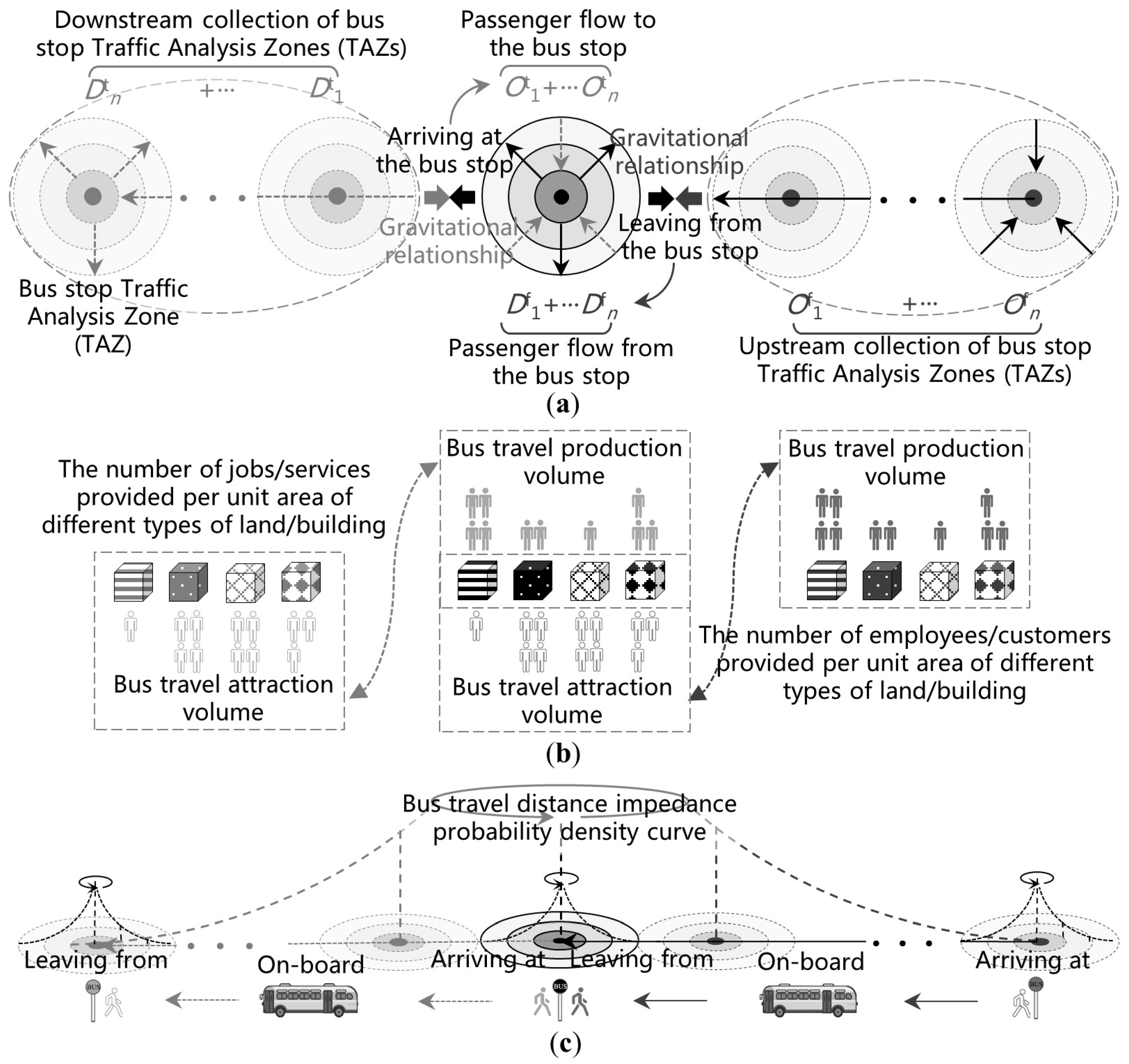
According to the gravity model principle mentioned above, the service area of a bus stop (serves multiple routes and nearby stops) can be regarded as a TAZ, specifically termed the bus stop TAZ. Passenger flow volumes from and to the bus stop correspond to the total bus travel volumes between the bus stop TAZ and its upstream and downstream collections of bus stop TAZs, as illustrated in Figure 1a. By translating the above corresponding relationship into the gravitational logic of bus travel, passenger flow volumes from and to the bus stop can be translated into bus travel generation and distance impedance based on land use elements between the experimental bus stop TAZ and its upstream and downstream collections of bus stop TAZs, as depicted in Figure 1.
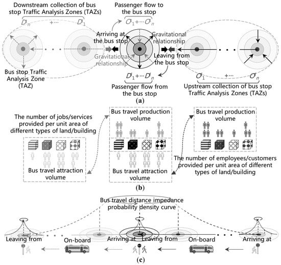
Figure 1.
Schematic of the estimation method for passenger flow volumes from and to bus stops: (a) illustration of the gravitational relationship of passenger flow volumes from and to the bus stop; (b) bus travel generation of area-based origin unit method; (c) bus travel distance impedance of probability density method.
As commonly understood, the primary bus travel demand of residents within a specific area and time remains relatively stable, alongside a similar stability in the correlation between land use (building space) catering to residents’ activity requirements and the number of activities. Therefore, bus travel generation is closely correlated with land use types and their area scales (intensities), which can be effectively aggregated using the area-based origin unit method. This method treats areas of the same land use type as homogeneous under certain conditions, while considering the average production and attraction volume of bus travel per unit area of land use or building, as illustrated in Figure 1b. Similarly, the correlation between residents’ bus travel spatial distributions and the proportionate distribution of residents’ bus travel distance remains relatively stable. Therefore, bus travel distance impedance is closely correlated with land use spatial distributions. It can be effectively aggregated using the probability density method, which deciphers the decay probability of different bus travel distances under certain conditions [47]. Due to the complete process of bus travel includes the three stages of “to (from)–onboard–from (to)”, its distance impedance can be decomposed into “from and to” distance impedance related to land use around the bus stop and “on-board” distance impedance related to land use around the surrounding areas of the bus stops upstream and downstream, as illustrated in Figure 1c.
2.2. Travel Time and Distance Decay Law
The analysis [46] of the time and distance decay law contained within the proportionate distributions of residents’ travel time and distance (by a certain travel mode and for a certain purpose) that ensures relatively accurate estimation of bus travel distance impedance is a crucial theoretical basis for the estimation method proposed in this paper. The research process is depicted in Figure 2.
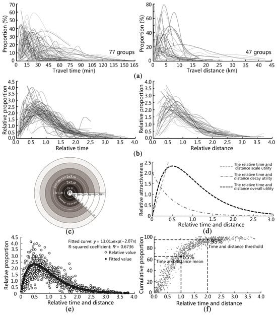
Figure 2.
The research process of the residents’ travel time and distance distribution law: (a) 124 groups of residents’ travel time and distance distributions; (b) relative time and distance distribution; (c) schematic of the relative time and distance scale utility; (d) schematic of the utility relationship of relative time and distance; (e) regression fitting curve of relative time and distance distribution; (f) cumulative proportional distribution of relative time and distance.
Firstly, the 124 groups of residents’ travel time and distance distributions with significant differences depicted in Figure 2a were standardized relative to their own mean travel time and distance, resulting in the stable and regular law of residents’ travel time and distance distributions relative to their mean values, as shown in Figure 2b. From the holistic spatiotemporal perspective of “supply–travel time and distance–demand”, the relative time and distance distribution abstractly represents an attraction relationship between standard supply and demand within the context of relative time and distance, while twice the mean of travel time and distance abstractly represents the scale of the supply–demand domain.
Secondly, the explanatory mechanism for the relative time and distance distribution shown in Figure 2d was constructed based on the utility of relative time and distance scale (illustrated in Figure 2c) and the utility of relative time and distance decay. For a facility point P in Figure 2c, the demand from individuals from different layers of relative time and distance (denoted as x) should exhibit a scale growth proportional to 2πx. However, due to the influence of relative time and distance decay following a pattern of λexp(−λx), the distribution stabilizes as depicted in Figure 2d.
Finally, the relative time and distance distribution data shown in Figure 2b were fitted with the equation y = 2πx⋅λexp(−λx), validating the interpretability of the relative time and distance distribution mechanism (as seen in Figure 2e), and yielding a relative time and distance decay parameter λ of 2.07 (after adjustment, the parameter value is 2.08). Additionally, from the cumulative proportion distribution of relative time and distance shown in Figure 2f, it was deduced that the threshold of resident travel time and distance is twice the mean travel time and distance.
3. Experimental Methods and Materials
3.1. The Estimation Method of Passenger Flow Volumes from and to Bus Stops
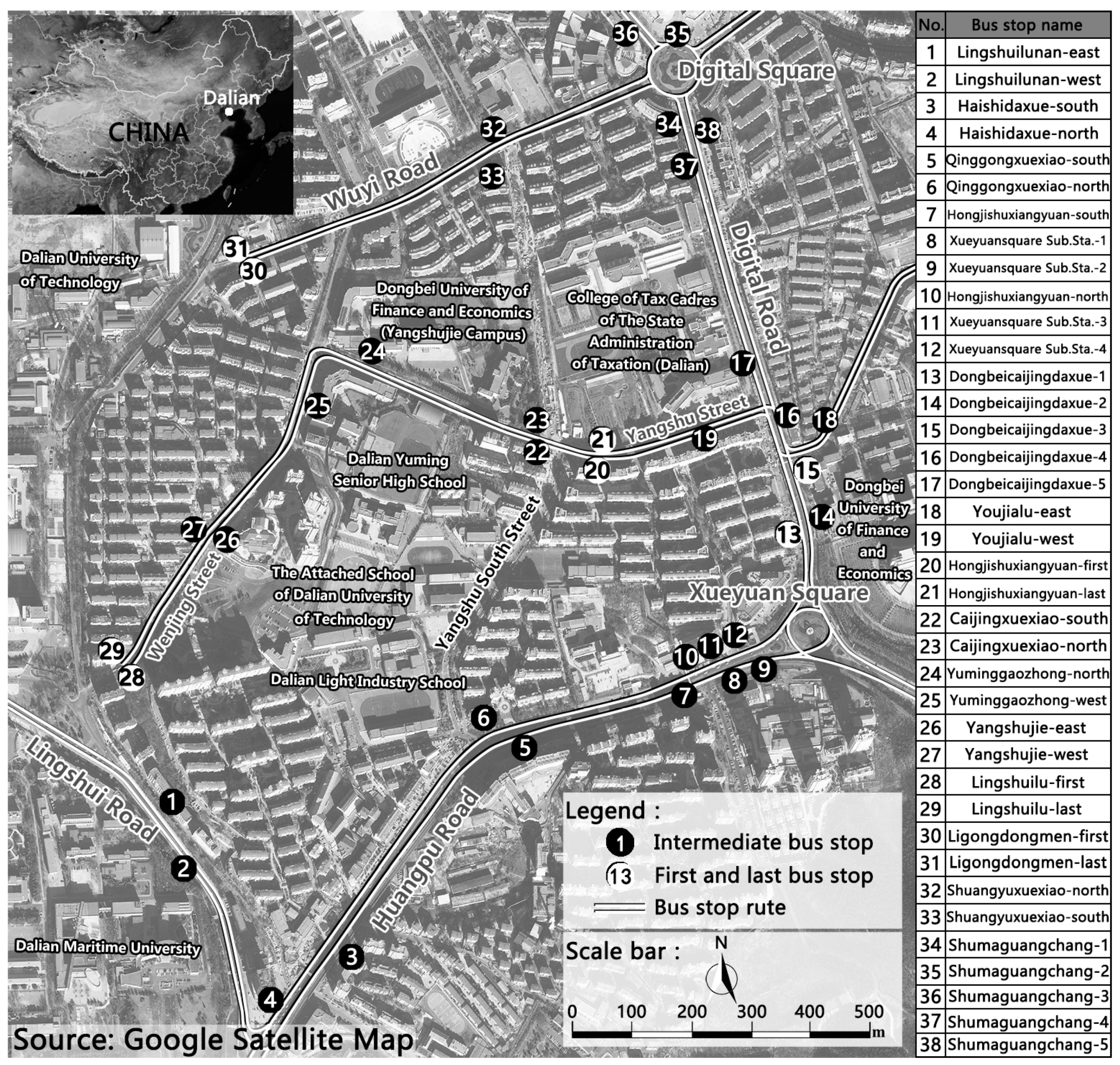
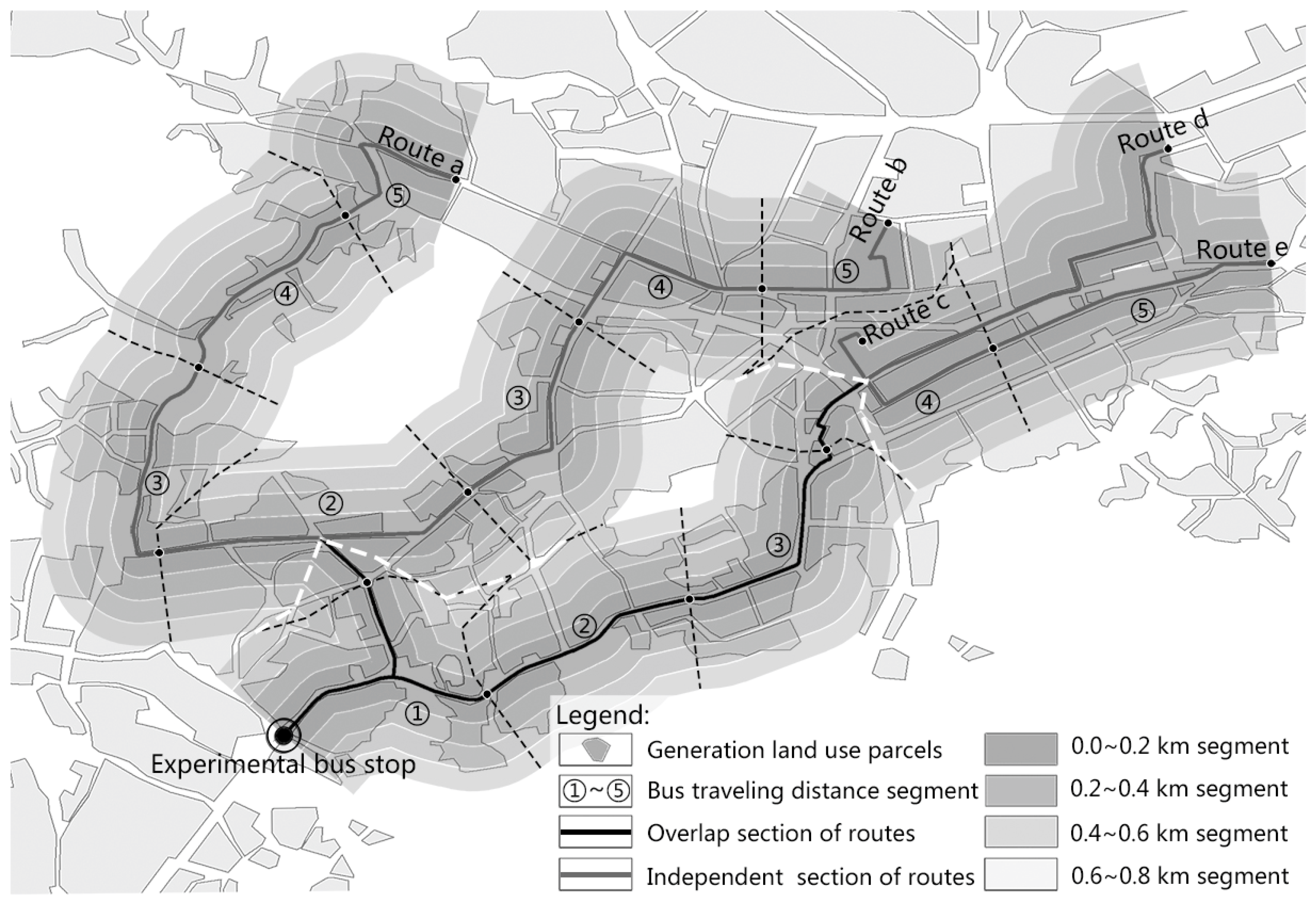
Building on the aforementioned estimation principle, this paper selects 19 pairs of conventional bus stops (totaling 38 bus stops as shown in Figure 3) in the Xueyuan Square area of Dalian, Liaoning Province, China, as experimental subjects, takes the passenger flow volumes from and to these bus stops during weekday morning peak hours (primarily for commuting) as estimation objects, and aims to examine the feasibility and effectiveness of the estimation principle and method by constructing an estimation model of passenger flow volumes based on land use between the experimental bus stop TAZs and upstream and downstream collections of bus stop TAZs.
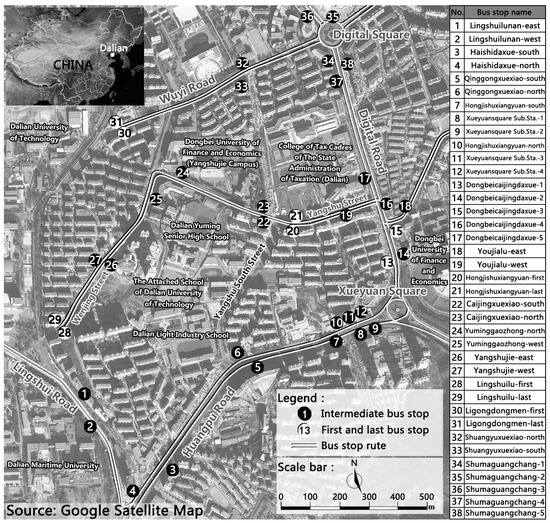
Figure 3.
Distribution of 38 experimental bus stops.
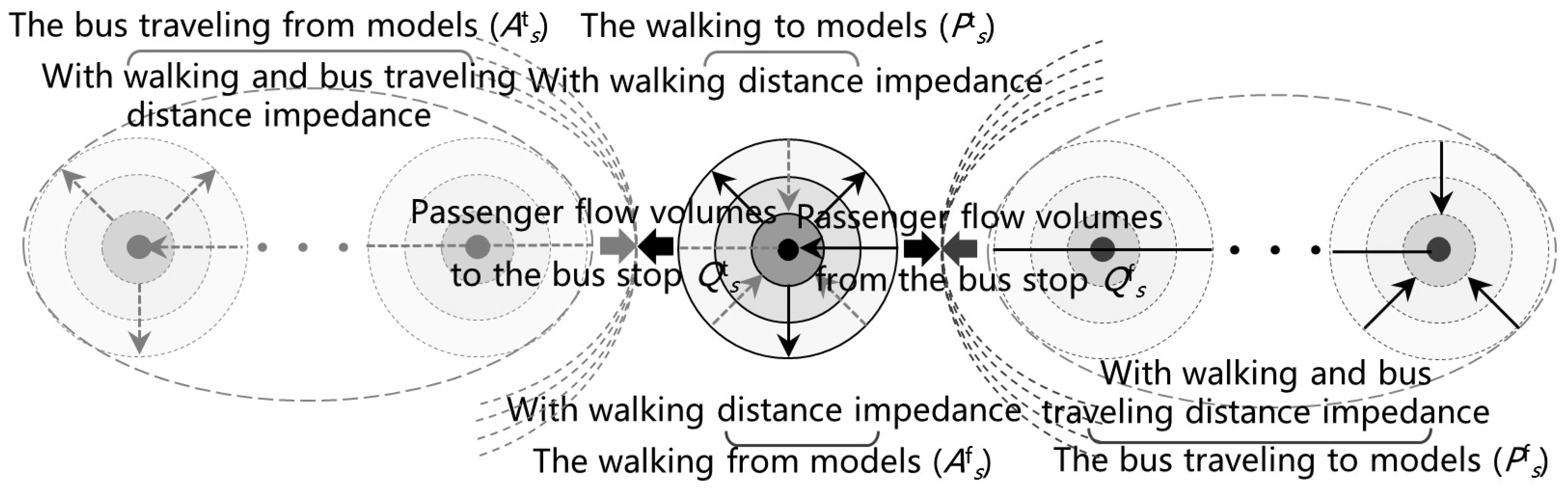
By treating passenger flow volumes from and to bus stops as analogous to gravitational forces between the experimental bus stop TAZs and their respective upstream and downstream collections of bus stop TAZs, the estimation model can be broken down into two gravity sets: the walking from-and-to models, which account for walking distance impedance within the experimental bus stop TAZs (since walking constitutes the absolute majority of travel from and to the bus stops in the survey area); and the bus travel from-and-to models, which incorporate bus travel distance impedance within the upstream and downstream bus stop TAZs. In this context, the corresponding relationship is illustrated in Figure 4, and the model formulas are expressed as Equations (2) and (3):
Qfs = Afs⋅Pfs
Qts = Pts⋅Ats

Figure 4.
Schematic of the estimation method of passenger flow volumes from and to bus stops.
In Equations (2) and (3), Qfs represents the passenger flow volumes from the bus stops, where “s” is the number of experimental bus stops and “f” stands for “from”, measured in passengers per hour (p⋅h−1); Afs represents the “walking from” models; Pfs represents the “bus travel to” models; Qts represents the passenger flow volumes to the bus stops, where “t” stands for “to”, measured in passengers per hour (p⋅h−1); Pts represents the “walking to” models; and Ats represents the “bus travel from” models.
3.2. Key Data for the Estimation Method
3.2.1. Passenger Flow Volumes from and to Bus Stops
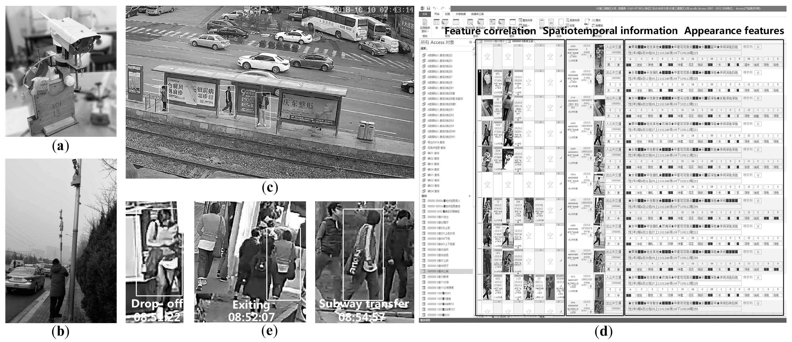
The passenger flow volumes from and to experimental bus stops during weekday morning peak hours, which are the objects of fitting and validating the estimation model (corresponding to two basic estimation models), can be obtained by deducting the transfer passenger flow volumes from the drop-off and pick-up passenger flow volumes of experimental bus stops. Following the experimental design, the process for obtaining these volumes is outlined below, with Figure 5 illustrating the relevant content.
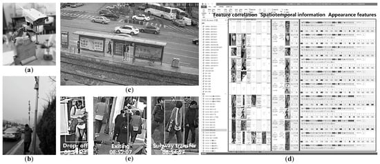
Figure 5.
Description of relevant content of passenger flow volume survey: (a) video equipment; (b) equipment setup; (c) video footage; (d) the Access database containing appearance features; (e) schematic of a transferring passenger.
Firstly, from 10 to 11 October 2018, video surveillance was conducted at 38 experimental bus stops and 1 transfer subway station (Xueyuan Square) to capture passenger flow information. The video equipment is shown in Figure 5a, the equipment setup is shown in Figure 5b, and the video footage is shown in Figure 5c.
Secondly, images and spatiotemporal information of drop-off and pick-up of passengers at each bus stop and the transfer subway station were captured and annotated during the morning peak hours (from 07:00 to 09:00) over the two days, as shown in Figure 5d.
Finally, based on the technique of pedestrian appearance feature re-identification, an Access database containing appearance features such as age, gender, attire, headwear, hairstyle, and carried items was constructed. Through feature correlation queries traversing image data, it identified transferring passengers, including both intra-stop transfers and inter-stop transfers, among drop-off and pick-up passengers of bus stops (as shown in Figure 5e). The final passenger flow volumes were calculated using the following Equations (4) and (5), with the corresponding survey data shown in Table A2 of Appendix A.
Qfs = Gfs − Hfs,
Qts = Gts − Hts,
In Equations (4) and (5), Gfs and Gts represent the drop-off and pick-up passenger flow volumes, respectively, during the morning peak hours, measured in passengers per hour (p⋅h−1). Hfs and Hts represent the drop-off and pick-up transfer passenger flow volumes, respectively, during the morning peak hours, measured in passengers per hour (p⋅h−1).
3.2.2. Walking and Bus Travel Distance Impedance
Based on the distribution law of residents’ travel time and distance mentioned above, the distance thresholds and the distance decay probabilities of walking and bus travel from and to the experimental bus stops, which correspond to the impact range of land use and distance impedance in the method proposed in this paper, can be obtained through a questionnaire survey on residents’ walking and bus travel distance from and to bus stops during the morning peak hours in the research area, conducted simultaneously with video surveillance. We collected 158 valid questionnaires, and the corresponding distribution results, along with their distance thresholds and impedances, are shown in Figure 6.
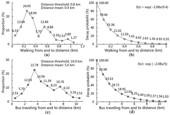
Figure 6.
Survey results along with distance thresholds and impedance: (a) walking from-and-to distance distribution; (b) walking from-and-to distance impedance; (c) bus travel from-and-to distance distribution; (d) bus travel from-and-to distance impedance.
According to the survey results shown in Figure 6a,c, the mean distances of walking and bus travel from-and-to distance distributions are 0.4 km and 5.0 km, respectively. Consequently, the distance threshold for walking from and to experimental bus stops is set at 0.8 km, with the probability distance impedance function represented as exp(−2.08x/0.4), while the distance threshold for bus travel from and to experimental bus stops is set at 10.0 km, with the probability distance impedance function represented as exp(−2.08x/5).
3.3. Construction of the Basic Estimation Models
3.3.1. The Walking from-and-to Models
The walking from-and-to models correspond to the gravity set associated with the generation and distance impedance of land use within the 38 experimental bus stop TAZs. Taking into account considerations such as the commuting and schooling service characteristics of bus travel during the morning peak hours, as well as the moderate simplification of the aggregation models, the generation estimation in the area-based origin unit method categorizes land use within experimental TAZs into four types: educational, residential, office, and commercial land uses. Their building areas are then aggregated to calculate the production volume and attraction volumes of bus travel in TAZs.
In the distance impedance estimation using the probability density method, where the probability decay function and distance threshold for walking distance from and to the experimental bus stops are known, the walking from and to distances are uniformly segmented, and the median distance decay probability of each segment is used to estimate the spatial distance impedance within the walking from-and-to distance segment. Based on the actual conditions of land use, walking path, and the competitive relationship of the experimental bus stop services, this paper constructs the walking from (Afs) and to (Pts) models. The calculation formula and model example (Figure 7) are as follows:
Afs = Σni[Si⋅(MeiTe + MriTr + MoiTo + MciTc)],
Pts = Σni[Si⋅(MeiOe + MriOr + MoiOo + MciOc)],
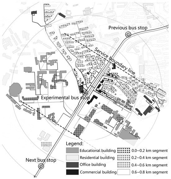
Figure 7.
Example of the generation and distance impedance of the walking from-and-to models.
In Equations (6) and (7), Si represents the distance decay probability for walking from-and-to distance segments, where i ranges from 1 to 4; Mei, Mri, Moi, and Mci represent the areas of educational, residential, office, and commercial buildings within the respective distance segments of bus stop TAZs, measured in hectares (ha); and Oe, Or, Oo, and Oc represent the relative bus travel production parameters, while Te, Tr, To, and Tc represent the relative bus travel attraction parameters, all measured in passengers per hectare per hour (P·h−1·ha−1), with “e”, “r”, “o”, and “c” denoting educational, residential, office, and commercial buildings, respectively.
3.3.2. The Bus Travel from-and-to Models
The bus travel from-and-to models correspond to the gravity set associated with the generation and distance impedance of land use within the upstream and downstream collections of bus stop TAZs. Considering that it is only necessary to simulate the total gravity of the gravity set, in the generation estimation using the area-based origin unit method, it may be feasible to treat educational, residential, office, and commercial land uses, collectively referred to as “generation land use”, within the service area of upstream and downstream collections of bus stop TAZs as homogeneous (fuzzy land use types, intensities, structure and spatial distributions without considering variations in generation parameters), and to take the area of “generation land use” to aggregate the production and attraction volumes of bus travel within the upstream and downstream collections of bus stop TAZs.
The distance impedance in the bus travel from-and-to models comprises two components: walking distance impedance and bus travel distance impedance within the upstream and downstream collections of bus stop TAZs. In the distance impedance estimation using the probability density method, the bus travel distance is evenly segmented, and a buffer is applied to the walking form and to distance. By combining the probabilities of both components, it becomes possible to estimate the spatial distance impedance within the bus travel from-and-to distance segment. This paper constructs the bus travel from (Pfs) and to (Ats) models based on the actual conditions of land use and bus route system within the upstream and downstream collections of bus stop TAZs. The calculation formula and a model example (Figure 8) are as follows:
Pfs = ΣniΣmj[Si⋅Rj⋅(h1Ffij + h2Nfij)],
Ats = ΣniΣmj[Si⋅Rj⋅(h1Ftij + h2Ntij)],
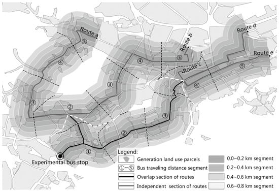
Figure 8.
Example of the generation and distance impedance of the bus travel from-and-to models.
In Equations (8) and (9), Rj represents the distance decay probability corresponding to the bus travel from-and-to distance segments, where j ranges from 1 to 5; Ffij, Nfij, Ftij, and Ntij represent the area of “generation land use” within the independent and overlapping regions (some experimental bus stops serve multiple bus routes, resulting in overlapping land use areas) within the buffer zones i and j, measured in square kilometers (km2); and h1 and h2 represent land use coefficients in these regions, set empirically to 1 and 2, respectively. This indicates that overlapping areas served by multiple routes are calculated at twice their per-unit area, measured in hectares per unit area (km−2).
4. Results
4.1. The Basic Estimation Models’ Parameters
Based on the construction of two basic estimation models, data from 38 experimental bus stops, corresponding to 68 groups (including 8 first or last bus stops with unidirectional data only), were investigated and collected, as shown in Table A1 and Table A2 of Appendix A. The decay probabilities of walking from-and-to distance segments, as well as bus travel from-and-to distance segments obtained from Figure 6, are presented in Table 1 and Table 2. By fitting the surveyed values of passenger flow volumes from and to 38 experimental bus stops with the basic estimation models, the relative production and attraction parameters of four types of land use (the unit building area) in the study area were determined, and the stepwise regression results are shown in Table 3 and Table 4.

Table 1.
The decay probabilities of walking from-and-to distance segments.
Table 2.
The decay probabilities of bus travel from-and-to distance segments.
Table 3.
The relative production parameters of four types of land use (the unit building area).
Table 4.
The relative attraction parameters of four types of land use (the unit building area).
4.2. Fit Validation of the Estimation Method
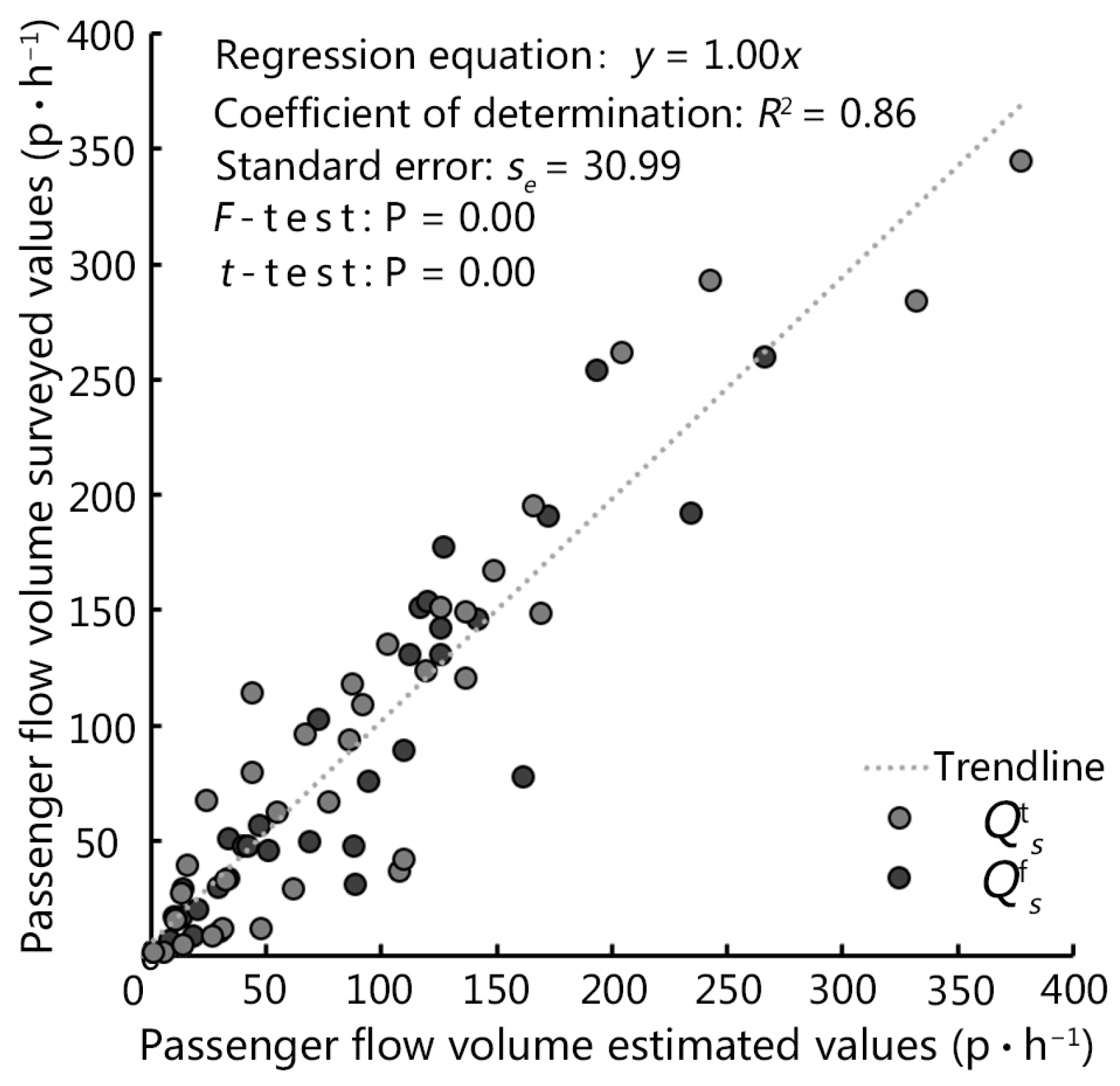
To test the explanatory power of the basic estimation models and validate the feasibility of the estimation method of passenger flow volumes from and to bus stops based on land use elements, a linear regression analysis was conducted between the surveyed values of passenger flow volumes of the 68 groups and the models’ estimated values (the related data are shown in Table A2 of Appendix A), which can demonstrate the correlation between the two sets of values. The results are shown in Figure 9.
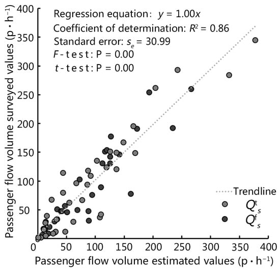
Figure 9.
Regression of the surveyed values and estimated values of passenger flow volumes from and to bus stops.
The correlation analysis in Figure 9 shows a strong linear relationship between estimated and surveyed values, represented by the equation y = 1.00x. With an R2 of 0.86, the model provides a good fit, indicating that estimated values have a high explanatory power for surveyed values. Additionally, both the F-test (F = 1007.25, p < 0.05) and t-test (t = 31.74, p < 0.05) confirm the validity of the linear regression model. These regression tests suggest the feasibility of the estimation method of passenger flow volumes from and to bus stops based on land use elements proposed in this paper. In essence, there exists a general relationship between bus travel and land use around bus stops and along bus routes, and passenger flow volumes from and to bus stops can be understood based on logical relationships between land use types, intensities, and spatial distributions. Furthermore, the combination of area-based origin unit method and distance impedance of probability density method effectively transforms this relationship.
5. Discussion
The construction of the gravitational logic of bus travel at the land use level using the bus travel generation aggregation of area-based origin unit method and the bus travel distance impedance of probability density method offers a theoretical foundation and methodological support for fostering fair [48,49], orderly [50], efficient, sustainable [51], and intensified demand organization in TOD.
The bus travel relative generation parameters (corresponding to generation efficiency) of different land use types in unit area and the bus travel relative distance decay law (corresponding to distance impedance, related to bus travel distance service levels), provide an orderly framework for coordinated development between land use and bus travel. In station area TOD, the basic unit order logic includes, the land use type layout should be organized based on generation efficiency to meet the bus travel intensity, and the same type of land use should follow a fair layout to reduce the impact of accessibility differences on travel efficiency. In citywide TOD, the order between basic units includes, the urban spatial functions should be relatively balanced to reduce pendulum-like commuting and the separation of residential and workplace areas, and the urban spatial structures should align with the operational characteristics (volume, speed, distance traveled, etc.) of different transportation systems to adapt to the structured upgrading of demand organization.
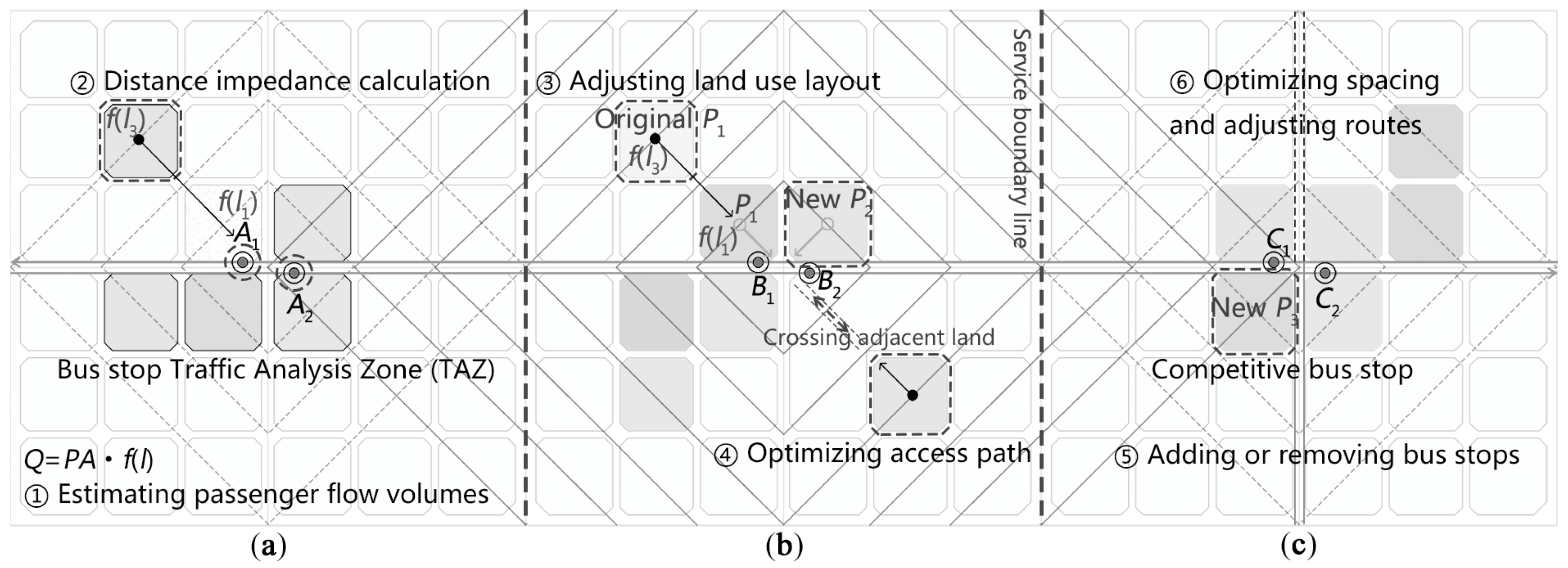
The construction of the estimation method of passenger flow volumes from and to bus stops provides actionable ideas for the straightforward analysis and optimization of TOD-related issues, as shown in Figure 10.
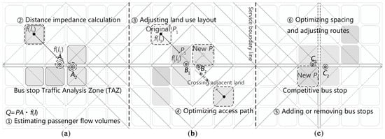
Figure 10.
Application scenarios of the estimation method.
As depicted in Figure 10, within the constraints of the study area and time period and with the calibration of parameters such as production, attraction, and distance impedance in the basic estimation models, the application scenarios of the estimation method may include three main categories, as follows.
(a) Estimating passenger flow volumes within bus stop TAZs: When the relationship between land use around bus stops and along bus routes is known, but passenger flow volumes from and to bus stops are unknown, this estimation method can be used to estimate these volumes and diagnose potential deficiencies in passenger flow in terms of land use types, intensities, and spatial distributions.
(b) Updating land use within bus stop TAZs for station area TOD: For bus stops where the relationship between land use around bus stops and along bus routes is known, this estimation method can not only assess walking inhibition from and to the bus stops (due to inconvenient paths, unreasonable layout relationship, etc.) under the current land use layout but also evaluate improvements in passenger flow volumes after adjusting land use layouts and optimizing access paths. This facilitates organic land use renewal within bus stop TAZs from a bus travel perspective.
(c) Updating land use within upstream and downstream bus stops TAZs for citywide TOD: For bus routes where the land use generation and distance impedance are known, the estimation method can not only assess the benefits in passenger flow volumes from scenarios such as adding or removing bus stops, optimizing spacing, and adjusting routes but also consider the redistribution of passenger flow volumes for integrated development in the service area and structural upgrades to meet increased demand.
6. Conclusions
To unravel the general relationship between bus travel and land use around bus stops and along bus routes and to foster their coordinated development, this paper explores the estimation method of passenger flow volumes from and to bus stops (serving as a link between the bus system and its service area) based on land use elements. Through the analysis of the gravity model principle and method of estimating passenger flow volumes, the construction of basic estimation models corresponding to the gravity set based on land use elements and empirical testing of the estimation method, the main conclusions obtained are as follows.
Regression results demonstrate the feasibility of estimating passenger flow volumes based on land use elements. In other words, passenger flow volumes from and to bus stops can be derived from the land use types, intensities, and spatial distributions on both sides connected by these volumes by treating the land use elements as the gravity set, which is related to the supply and demand of passenger flow volumes. Decoding this general relationship provides a fair and orderly methodological framework for the coordinated development and strategic decision-making on bus travel and land use around bus stops and along bus routes, particularly in the context of TOD planning updates.
In contrast to existing complex and non-transferable analytic predictions concerning bus network relationships, this paper introduces the concept of passenger flow volumes from and to bus stops, deconstructing the point–line units corresponding to these volumes from bus network relationships to simplify the estimation of passenger flow volumes at the land use level. By using the area-based origin unit method, which hypothesizes the bus travel generation is closely correlated with land use types and their corresponding area scales, and the bus travel distance impedance of probability density method, which deciphers the decay probability of different bus travel distances under certain conditions, a portable estimation method based on gravity relationships is constructed and empirically verified.
While the function model has been tested and confirmed with relatively high confidence, ensuring the reliability of the estimation approach and method, there are limitations in its application and extension. The estimation model primarily simulates passenger flow volumes from and to bus stops during the morning peak period in the experimental area, so future research should expand the study area and time period for broader verification of the estimation method. Additionally, the simplified basic estimation models used for experimentation may suffer from issues such as poor representativeness of parameter values, inadequate transfer considerations, and insufficient prediction accuracy. To improve the model, it is necessary to minimize the interference of random factors in estimation of passenger flow volumes from and to bus stops and refine the aggregation of generation and distance impedance while improving the aggregation of transfer passenger flow volumes of bus travel.
Author Contributions
Conceptualization, J.C.; methodology, software, and validation, J.Z.; formal analysis, J.Z. and M.W.; investigation, resources, and data curation, J.Z., J.C. and W.Z.; writing—original draft preparation, J.Z., W.Z. and M.W.; writing—review and editing, J.Z. and J.C.; visualization, J.Z.; supervision, project administration, and funding acquisition, J.Z. and J.C. All authors have read and agreed to the published version of the manuscript.
Funding
This research was funded by the National Natural Science Foundation of China, grant 52278048, project Research on Theory and Intelligent Method of Road Network Quality Improving Planning from the Perspective of Dual Motive of City and Block. The APC was funded by the National Natural Science Foundation of China.
Data Availability Statement
The data presented in this study are available upon request from the first author due to the complexity and privacy concerns associated with the raw data. Summary data supporting the study results can be found in Appendix A.
Acknowledgments
The authors sincerely thank the editors and reviewers for their valuable comments on this manuscript.
Conflicts of Interest
The authors declare no conflicts of interest.
Appendix A
Table A1.
Statistical data on building areas for four types of land use within four walking distance segments (km).
Table A1.
Statistical data on building areas for four types of land use within four walking distance segments (km).
| No. | Mei (ha) | Mri (ha) | Moi (ha) | Mci (ha) | ||||||||||||
|---|---|---|---|---|---|---|---|---|---|---|---|---|---|---|---|---|
| (0.0, 0.2) | (0.2, 0.4) | (0.4, 0.6) | (0.6, 0.8) | (0.0, 0.2) | (0.2, 0.4) | (0.4, 0.6) | (0.6, 0.8) | (0.0, 0.2) | (0.2, 0.4) | (0.4, 0.6) | (0.6, 0.8) | (0.0, 0.2) | (0.2, 0.4) | (0.4, 0.6) | (0.6, 0.8) | |
| 1 | 0.00 | 0.00 | 1.77 | 0.00 | 2.24 | 2.43 | 3.39 | 2.64 | 0.00 | 0.34 | 0.11 | 0.27 | 0.00 | 0.16 | 0.00 | 0.00 |
| 2 | 0.00 | 0.00 | 0.00 | 0.00 | 2.64 | 2.06 | 2.41 | 3.25 | 0.06 | 1.57 | 0.09 | 0.15 | 0.13 | 0.426 | 0.00 | 0.00 |
| 3 | 0.00 | 1.60 | 4.29 | 8.95 | 9.81 | 10.62 | 12.95 | 0.00 | 1.64 | 0.01 | 2.58 | 0.18 | 2.52 | 0.30 | 0.00 | 2.48 |
| 4 | 0.00 | 1.70 | 9.31 | 13.14 | 6.30 | 10.91 | 15.23 | 4.10 | 1.64 | 0.01 | 1.05 | 2.76 | 2.31 | 0.54 | 0.04 | 0.00 |
| 5 | 0.96 | 11.93 | 1.18 | 5.11 | 5.91 | 6.23 | 11.59 | 7.73 | 0.99 | 0.00 | 1.14 | 0.00 | 0.04 | 0.17 | 0.00 | 0.00 |
| 6 | 2.51 | 7.13 | 4.27 | 0.61 | 1.90 | 8.21 | 14.84 | 4.17 | 0.99 | 0.00 | 1.14 | 0.00 | 0.00 | 0.11 | 0.10 | 0.32 |
| 7 | 0.00 | 5.82 | 2.54 | 0.00 | 5.08 | 23.00 | 9.90 | 7.29 | 1.04 | 1.99 | 0.96 | 0.11 | 1.32 | 0.76 | 0.24 | 0.07 |
| 8 | 0.00 | 0.79 | 12.35 | 12.76 | 0.00 | 14.21 | 26.22 | 14.52 | 0.29 | 2.76 | 0.00 | 0.962 | 3.31 | 1.89 | 1.71 | 0.18 |
| 9 | 0.00 | 0.79 | 12.35 | 12.76 | 0.00 | 14.21 | 26.22 | 14.52 | 0.29 | 2.76 | 0.00 | 0.96 | 3.31 | 1.89 | 1.71 | 0.18 |
| 10 | 0.00 | 5.82 | 2.54 | 0.00 | 5.08 | 23.00 | 9.90 | 7.29 | 1.04 | 1.99 | 0.96 | 0.11 | 1.32 | 0.76 | 0.24 | 0.07 |
| 11 | 0.00 | 0.79 | 12.35 | 12.76 | 0.00 | 14.21 | 26.22 | 14.52 | 0.29 | 2.76 | 0.00 | 0.96 | 3.31 | 1.89 | 1.71 | 0.18 |
| 12 | 0.00 | 0.79 | 12.35 | 12.76 | 0.00 | 14.21 | 26.22 | 14.52 | 0.29 | 2.76 | 0.00 | 0.96 | 3.31 | 1.89 | 1.71 | 0.18 |
| 13 | 1.42 | 5.37 | 10.12 | 15.25 | 2.22 | 9.92 | 22.37 | 12.44 | 0.00 | 0.20 | 2.74 | 0.26 | 3.76 | 2.86 | 0.29 | 0.49 |
| 14 | 1.42 | 5.37 | 10.12 | 15.25 | 2.22 | 9.92 | 22.37 | 12.44 | 0.00 | 0.20 | 2.74 | 0.26 | 3.76 | 2.86 | 0.29 | 0.49 |
| 15 | 1.42 | 5.37 | 10.12 | 15.25 | 2.22 | 9.92 | 22.37 | 12.44 | 0.00 | 0.20 | 2.74 | 0.26 | 3.76 | 2.86 | 0.29 | 0.49 |
| 16 | 2.21 | 9.56 | 13.39 | 14.13 | 6.45 | 8.69 | 4.71 | 0.00 | 0.00 | 0.10 | 0.00 | 0.00 | 2.42 | 0.89 | 0.18 | 0.00 |
| 17 | 1.47 | 6.75 | 11.45 | 11.94 | 6.08 | 9.40 | 4.38 | 1.06 | 0.00 | 0.22 | 0.00 | 1.83 | 1.37 | 1.85 | 0.21 | 0.00 |
| 18 | 4.16 | 7.41 | 8.75 | 0.66 | 2.88 | 9.01 | 3.75 | 4.55 | 0.00 | 0.10 | 0.00 | 3.97 | 1.39 | 4.28 | 1.95 | 0.38 |
| 19 | 2.83 | 8.10 | 2.47 | 1.62 | 6.95 | 9.77 | 5.74 | 2.44 | 0.00 | 0.10 | 0.00 | 2.047 | 2.84 | 2.77 | 1.95 | 0.38 |
| 20 | 0.00 | 7.85 | 13.47 | 4.14 | 10.27 | 10.02 | 9.09 | 14.94 | 0.00 | 0.00 | 0.00 | 2.05 | 0.18 | 2.80 | 3.43 | 0.73 |
| 21 | 0.00 | 7.85 | 13.47 | 4.14 | 10.27 | 10.02 | 9.09 | 14.94 | 0.00 | 0.00 | 0.00 | 2.05 | 0.18 | 2.80 | 3.43 | 0.73 |
| 22 | 1.02 | 5.00 | 3.25 | 7.83 | 6.76 | 5.33 | 13.39 | 3.87 | 0.00 | 0.00 | 0.16 | 2.46 | 0.18 | 0.00 | 0.19 | 0.11 |
| 23 | 1.02 | 5.00 | 3.25 | 7.83 | 6.76 | 5.33 | 13.39 | 3.87 | 0.00 | 0.00 | 0.16 | 2.46 | 0.18 | 0.00 | 0.19 | 0.11 |
| 24 | 4.63 | 1.11 | 0.00 | 0.00 | 0.86 | 6.35 | 2.26 | 5.65 | 0.00 | 0.04 | 0.45 | 1.04 | 0.06 | 0.32 | 0.11 | 0.05 |
| 25 | 3.41 | 1.92 | 4.73 | 6.02 | 4.38 | 11.47 | 6.62 | 5.78 | 0.04 | 0.04 | 2.67 | 0.58 | 0.06 | 0.71 | 0.08 | 0.05 |
| 26 | 0.00 | 0.00 | 3.53 | 2.41 | 5.18 | 2.11 | 0.00 | 0.00 | 0.20 | 0.19 | 0.00 | 0.00 | 0.09 | 0.39 | 0.00 | 0.00 |
| 27 | 0.00 | 0.00 | 3.53 | 2.41 | 5.18 | 2.11 | 0.00 | 0.00 | 0.20 | 0.19 | 0.00 | 0.00 | 0.09 | 0.39 | 0.00 | 0.00 |
| 28 | 0.00 | 1.77 | 2.21 | 1.12 | 4.38 | 4.01 | 0.92 | 3.98 | 0.10 | 0.97 | 0.06 | 1.60 | 0.05 | 0.17 | 1.92 | 2.55 |
| 29 | 0.00 | 1.77 | 2.21 | 1.12 | 4.38 | 4.01 | 0.92 | 3.98 | 0.10 | 0.97 | 0.06 | 1.60 | 0.05 | 0.17 | 1.92 | 2.55 |
| 30 | 0.14 | 9.90 | 15.06 | 15.25 | 3.66 | 11.93 | 5.64 | 9.48 | 0.04 | 0.14 | 1.17 | 0.22 | 0.71 | 0.11 | 0.00 | 0.12 |
| 31 | 0.14 | 9.90 | 15.06 | 15.25 | 3.66 | 11.93 | 5.64 | 9.48 | 0.04 | 0.14 | 1.17 | 0.22 | 0.71 | 0.11 | 0.00 | 0.12 |
| 32 | 1.32 | 1.62 | 0.07 | 0.00 | 6.21 | 11.03 | 9.97 | 8.79 | 1.37 | 1.64 | 0.57 | 1.73 | 0.20 | 0.26 | 0.25 | 1.74 |
| 33 | 1.32 | 1.62 | 0.07 | 0.00 | 6.21 | 11.03 | 9.97 | 8.79 | 1.37 | 1.64 | 0.57 | 1.73 | 0.20 | 0.26 | 0.25 | 1.74 |
| 34 | 0.00 | 3.76 | 0.38 | 0.00 | 8.11 | 18.58 | 23.48 | 18.89 | 2.54 | 0.00 | 8.79 | 6.83 | 0.60 | 2.28 | 1.17 | 0.20 |
| 35 | 1.39 | 2.75 | 0.00 | 0.00 | 8.84 | 26.21 | 19.23 | 5.42 | 2.54 | 3.36 | 11.26 | 1.53 | 1.71 | 1.75 | 0.35 | 0.11 |
| 36 | 1.39 | 2.75 | 0.00 | 0.00 | 8.84 | 26.21 | 19.23 | 5.42 | 2.54 | 3.36 | 11.26 | 1.53 | 1.71 | 1.75 | 0.35 | 0.11 |
| 37 | 0.00 | 3.01 | 1.13 | 0.00 | 5.99 | 20.29 | 16.50 | 15.82 | 2.54 | 0.00 | 8.38 | 4.98 | 0.60 | 2.69 | 0.53 | 0.09 |
| 38 | 0.00 | 3.01 | 1.13 | 0.00 | 5.99 | 20.29 | 16.50 | 15.82 | 2.54 | 0.00 | 8.38 | 4.98 | 0.60 | 2.69 | 0.53 | 0.09 |
Table A2.
Surveyed values of passenger flow volumes and models’ estimated values (including aggregate data from two basic models).
Table A2.
Surveyed values of passenger flow volumes and models’ estimated values (including aggregate data from two basic models).
| No. | Mei⋅Si (ha) | Mri⋅Si (ha) | Moi⋅Si (ha) | Mci⋅Si (ha) | Afs (P·h−1) | Pfs | Afs⋅Pfs (P·h−1) | Qfs (P·h−1) | Pts (P·h−1) | Ats | Pts⋅Ats (P·h−1) | Qts (P·h−1) |
|---|---|---|---|---|---|---|---|---|---|---|---|---|
| 1 | 0.13 | 2.16 | 0.09 | 0.03 | 13.26 | 0.99 | 13.2 | 17.0 | 15.49 | 0.86 | 13.3 | 27.5 |
| 2 | 0.00 | 2.27 | 0.37 | 0.17 | 21.62 | 0.86 | 18.5 | 8.5 | 31.19 | 0.99 | 31.0 | 12.0 |
| 3 | 0.89 | 9.03 | 1.17 | 1.63 | 108.39 | 1.59 | 172.7 | 191.0 | 133.00 | 1.82 | 242.5 | 293.0 |
| 4 | 1.40 | 7.28 | 1.13 | 1.49 | 106.09 | 1.82 | 193.4 | 254.0 | 128.29 | 1.59 | 204.3 | 262.0 |
| 5 | 3.30 | 5.89 | 0.67 | 0.06 | 94.19 | 1.72 | 161.9 | 78.0 | 103.89 | 1.63 | 169.0 | 149.0 |
| 6 | 3.33 | 4.07 | 0.67 | 0.04 | 87.22 | 1.63 | 141.8 | 146.0 | 96.53 | 1.72 | 165.9 | 195.0 |
| 7 | 1.41 | 8.78 | 1.11 | 0.97 | 102.64 | 0.87 | 89.0 | 31.0 | 126.33 | 0.86 | 108.2 | 37.0 |
| 8 | 1.42 | 5.32 | 0.78 | 2.49 | 106.91 | 1.17 | 125.5 | 131.0 | 116.44 | 1.03 | 119.6 | 124.0 |
| 9 | 1.42 | 5.32 | 0.78 | 2.49 | 106.91 | 1.18 | 125.7 | 142.0 | 116.44 | 0.88 | 103.0 | 135.0 |
| 10 | 1.41 | 8.78 | 1.11 | 0.97 | 102.64 | 0.86 | 87.9 | 48.0 | 126.33 | 0.87 | 109.5 | 42.0 |
| 11 | 1.42 | 5.32 | 0.78 | 2.49 | 106.91 | 1.03 | 109.8 | 89.0 | 116.44 | 1.17 | 136.7 | 149.5 |
| 12 | 1.42 | 5.32 | 0.778 | 2.49 | 106.91 | 0.88 | 94.5 | 76.0 | 116.44 | 1.18 | 136.9 | 120.5 |
| 13 | 3.12 | 5.40 | 0.25 | 2.87 | 126.75 | 0.57 | 72.5 | 103.0 | — | — | — | — |
| 14 | 3.12 | 5.40 | 0.25 | 2.87 | 126.75 | 0.92 | 117.1 | 151.0 | 117.18 | 1.07 | 125.7 | 151.0 |
| 15 | 3.12 | 5.40 | 0.25 | 2.87 | — | — | — | — | 117.18 | 0.57 | 67.0 | 96.5 |
| 16 | 4.69 | 6.02 | 0.02 | 1.64 | 126.52 | 0.89 | 112.2 | 130.5 | 110.89 | 0.70 | 77.3 | 67.0 |
| 17 | 3.46 | 5.95 | 0.09 | 1.22 | 101.28 | 1.26 | 127.1 | 177.5 | 92.08 | 1.61 | 148.6 | 167.5 |
| 18 | 4.70 | 4.01 | 0.12 | 1.88 | 125.90 | 0.55 | 68.8 | 49.5 | 111.75 | 0.24 | 26.6 | 8.5 |
| 19 | 3.61 | 6.68 | 0.07 | 2.43 | 126.87 | 0.24 | 30.2 | 10.5 | 113.10 | 0.55 | 61.8 | 29.0 |
| 20 | 2.76 | 9.28 | 0.05 | 0.97 | — | — | — | — | 90.61 | 0.53 | 47.6 | 12.0 |
| 21 | 2.76 | 9.28 | 0.05 | 0.97 | 97.55 | 0.53 | 51.3 | 46.0 | — | — | — | — |
| 22 | 2.11 | 6.24 | 0.08 | 0.12 | 61.53 | 0.18 | 11.0 | 15.5 | 58.91 | 0.55 | 32.3 | 33.0 |
| 23 | 2.11 | 6.24 | 0.08 | 0.12 | 61.53 | 0.55 | 33.7 | 34.0 | 58.91 | 0.18 | 10.5 | 15.5 |
| 24 | 2.99 | 2.16 | 0.07 | 0.11 | 59.57 | 0.57 | 34.1 | 51.0 | 53.65 | 0.10 | 5.4 | 2.0 |
| 25 | 2.94 | 5.66 | 0.25 | 0.19 | 78.32 | 0.10 | 7.9 | 7.0 | 77.52 | 0.57 | 44.3 | 80.0 |
| 26 | 0.33 | 3.52 | 0.16 | 0.14 | 25.21 | 0.04 | 1.0 | 2.0 | 28.70 | 0.56 | 16.1 | 39.5 |
| 27 | 0.33 | 3.52 | 0.16 | 0.14 | 25.21 | 0.56 | 14.1 | 29.0 | 28.70 | 0.04 | 1.1 | 2.0 |
| 28 | 0.57 | 3.62 | 0.31 | 0.28 | — | — | — | — | 42.40 | 0.57 | 24.1 | 67.5 |
| 29 | 0.57 | 3.62 | 0.31 | 0.28 | 35.97 | 0.57 | 20.4 | 20.5 | — | — | — | — |
| 30 | 3.68 | 5.35 | 0.14 | 0.45 | — | — | — | — | 84.40 | 0.52 | 44.2 | 114.0 |
| 31 | 3.68 | 5.35 | 0.14 | 0.45 | 90.62 | 0.52 | 47.4 | 56.5 | — | — | — | — |
| 32 | 1.13 | 6.98 | 1.25 | 0.24 | 82.36 | 0.49 | 40.3 | 47.5 | 112.21 | 0.12 | 13.9 | 5.0 |
| 33 | 1.13 | 6.98 | 1.25 | 0.24 | 82.36 | 0.12 | 10.2 | 17.0 | 112.21 | 0.49 | 54.9 | 62.5 |
| 34 | 0.82 | 10.97 | 2.34 | 0.93 | 134.10 | 0.22 | 29.4 | 30.0 | 191.55 | 0.48 | 91.7 | 109.0 |
| 35 | 1.41 | 12.34 | 3.09 | 1.41 | 177.19 | 1.50 | 266.5 | 260.0 | 251.15 | 1.32 | 332.3 | 284.0 |
| 36 | 1.41 | 12.34 | 3.09 | 1.41 | 177.19 | 1.32 | 234.5 | 192.0 | 251.15 | 1.50 | 377.8 | 344.5 |
| 37 | 0.72 | 9.47 | 2.26 | 0.97 | 125.23 | 0.34 | 42.3 | 48.0 | 180.50 | 0.48 | 86.5 | 94.0 |
| 38 | 0.72 | 9.47 | 2.26 | 0.97 | 125.23 | 0.96 | 119.9 | 154.0 | 180.50 | 0.49 | 87.6 | 118.0 |
References
- Berawi, M.A.; Saroji, G.; Iskandar, F.A.; Ibrahim, B.E.; Miraj, P.; Sari, M. Optimizing Land Use Allocation of Transit-Oriented Development (TOD) to Generate Maximum Ridership. Sustainability 2020, 12, 3798. [Google Scholar] [CrossRef]
- Hasibuan, H.S.; Mulyani, M. Transit-Oriented Development: Towards Achieving Sustainable Transport and Urban Development in Jakarta Metropolitan, Indonesia. Sustainability 2022, 14, 5244. [Google Scholar] [CrossRef]
- Woo, J.H. Classification of TOD Typologies Based on Pedestrian Behavior for Sustainable and Active Urban Growth in Seoul. Sustainability 2021, 13, 3047. [Google Scholar] [CrossRef]
- Stojanovski, T. Urban design and public transportation—Public spaces, visual proximity and Transit-Oriented Development (TOD). J. Urban Des. 2020, 25, 134–154. [Google Scholar]
- Su, S.; Zhang, J.; He, S.; Zhang, H.; Hu, L.; Kang, M. Unraveling the impact of TOD on housing rental prices and implications on spatial planning: A comparative analysis of five Chinese megacities. Habitat Int. 2021, 107, 102309. [Google Scholar] [CrossRef]
- Gan, Z.; Yang, M.; Feng, T.; Timmermans, H.P. Examining the relationship between built environment and metro ridership at station-to-station level. Transp. Res. D Transp. Environ. 2020, 82, 102332. [Google Scholar] [CrossRef]
- Newman, P.; Davies-Slate, S.; Conley, D.; Hargroves, K.; Mouritz, M. From TOD to TAC: Why and How Transport and Urban Policy Needs to Shift to Regenerating Main Road Corridors with New Transit Systems. Urban Sci. 2021, 5, 52. [Google Scholar] [CrossRef]
- Wang, B.; de Jong, M.; van Bueren, E.; Ersoy, A.; Meng, Y. Transit-Oriented Development in China: A Comparative Content Analysis of the Spatial Plans of High-Speed Railway Station Areas. Land 2023, 12, 1818. [Google Scholar] [CrossRef]
- Carlton, I. Transit Planners’ Transit-Oriented Development-Related Practices and Theories. J. Plan. Educ. Res. 2019, 39, 508–519. [Google Scholar] [CrossRef]
- Ibrahim, S.M.; Ayad, H.M.; Turki, E.A.; Saadallah, D.M. Measuring Transit-Oriented Development (TOD) levels: Prioritize potential areas for TOD in Alexandria, Egypt using GIS-Spatial Multi-Criteria based model. Alex. Eng. J. 2023, 67, 241–255. [Google Scholar] [CrossRef]
- Ibraeva, A.; de Almeida Correia, G.H.; Silva, C.; Antunes, A.P. Transit-oriented development: A review of research achievements and challenges. Transp. Res. Part A Policy Pract. 2020, 132, 110–130. [Google Scholar] [CrossRef]
- Su, S.; Zhao, C.; Zhou, H.; Li, B.; Kang, M. Unraveling the relative contribution of TOD structural factors to metro ridership: A novel localized modeling approach with implications on spatial planning. J. Transp. Geogr. 2022, 100, 103308. [Google Scholar] [CrossRef]
- Currie, G. Bus Transit Oriented Development—Strengths and Challenges Relative to Rail. J. Public Transp. 2006, 9, 1–21. [Google Scholar] [CrossRef]
- Shen, Q.; Xu, S.; Lin, J. Effects of bus transit-oriented development (BTOD) on single-family property value in Seattle metropolitan area. Urban Stud. 2018, 55, 2960–2979. [Google Scholar] [CrossRef]
- Pan, H.; Li, J.; Shen, Q.; Shi, C. What determines rail transit passenger volume? Implications for transit oriented development planning. Transp. Res. Part D Transp. Environ. 2017, 57, 52–63. [Google Scholar] [CrossRef]
- Huang, Y.; Zhang, Z.; Xu, Q.; Dai, S.; Chen, Y. Causality between multi-scale built environment and rail transit ridership in Beijing and Tokyo. Transp. Res. Part D Trans. Environ. 2024, 130, 104150. [Google Scholar] [CrossRef]
- Wegener, M. Land-Use Transport Interaction Models. In Handbook of Regional Science; Fischer, M., Nijkamp, P., Eds.; Springer: Berlin/Heidelberg, Germany, 2021; pp. 229–246. [Google Scholar] [CrossRef]
- Ren, F.; Zhang, J.; Yang, X. Study on the Effect of Job Accessibility and Residential Location on Housing Occupancy Rate: A Case Study of Xiamen, China. Land 2023, 12, 912. [Google Scholar] [CrossRef]
- Derakhti, L.; Baeten, G. Contradictions of Transit-Oriented Development in Low-Income Neighborhoods: The Case Study of Rosengård in Malmö, Sweden. Urban Sci. 2020, 4, 20. [Google Scholar] [CrossRef]
- Lin, C.; Wang, K.; Wu, D.; Gong, B. Passenger Flow Prediction Based on Land Use around Metro Stations: A Case Study. Sustainability 2020, 12, 6844. [Google Scholar] [CrossRef]
- Zhai, H.; Tian, R.; Cui, L.; Xu, X.; Zhang, W. A Novel Hierarchical Hybrid Model for Short-Term Bus Passenger Flow Forecasting. J. Adv. Transp. 2020, 2020, 7917353. [Google Scholar] [CrossRef]
- Zhang, X.; Yan, M.; Xie, B.; Yang, H.; Ma, H. An automatic real-time bus schedule redesign method based on bus arrival time prediction. Adv. Eng. Inform. 2021, 48, 101295. [Google Scholar] [CrossRef]
- Li, W.; Sui, L.; Zhou, M.; Dong, H. Short-term passenger flow forecast for urban rail transit based on multi-source data. EURASIP J. Wirel. Comm. 2021, 2021, 9. [Google Scholar] [CrossRef]
- Wen, K.; Zhao, G.; He, B.; Ma, J.; Zhang, H. A decomposition-based forecasting method with transfer learning for railway short-term passenger flow in holidays. Expert Syst. Appl. 2022, 189, 116102. [Google Scholar] [CrossRef]
- Liu, W.; Tan, Q.; Wu, W. Forecast and Early Warning of Regional Bus Passenger Flow Based on Machine Learning. Math. Probl. Eng. 2020, 2020, 6625435. [Google Scholar] [CrossRef]
- Baghbani, A.; Bouguila, N.; Patterson, Z. Short-Term Passenger Flow Prediction Using a Bus Network Graph Convolutional Long Short-Term Memory Neural Network Model. Transp. Res. Rec. 2023, 2677, 1331–1340. [Google Scholar] [CrossRef]
- Liu, L.; Chen, R. A novel passenger flow prediction model using deep learning methods. Transp. Res. Part C Emerg. Technol. 2017, 84, 74–91. [Google Scholar] [CrossRef]
- Halyal, S.; Mulangi, R.H.; Harsha, M.M. Forecasting public transit passenger demand: With neural networks using APC data. Case Stud. 2022, 10, 965–975. [Google Scholar] [CrossRef]
- Arhin, S.; Manandhar, B.; Baba-Adam, H. Predicting Travel Times of Bus Transit in Washington, D.C. Using Artificial Neural Networks. Civ. Eng. J. 2020, 6, 2245–2261. [Google Scholar] [CrossRef]
- Lv, W.; Lv, Y.; Ouyang, Q.; Ren, Y. A Bus Passenger Flow Prediction Model Fused with Point-of-Interest Data Based on Extreme Gradient Boosting. Appl. Sci. 2022, 12, 940. [Google Scholar] [CrossRef]
- Deepa, L.; Pinjari, A.R.; Nirmale, S.K.; Srinivasan, K.K.; Rambha, T. A direct demand model for bus transit ridership in Bengaluru, India. Transp. Res. Part A Policy Pract. 2022, 163, 126–147. [Google Scholar] [CrossRef]
- Klar, B.; Lee, J.; Long, J.A.; Diab, E. The impacts of accessibility measure choice on public transit project evaluation: A comparative study of cumulative, gravity-based, and hybrid approaches. J. Transp. Geogr. 2023, 106, 103508. [Google Scholar] [CrossRef]
- Lee, J.H.; Kim, J.W.; Lee, K.; Choi, M.Y. Generalized maximal entropy argument for the gravity law in human mobility. Europhys. Lett. 2020, 132, 48001. [Google Scholar] [CrossRef]
- Zhang, N.; Wang, Z.; Chen, F.; Song, J.; Wang, J.; Li, Y. Low-Carbon Impact of Urban Rail Transit Based on Passenger Demand Forecast in Baoji. Energies 2020, 13, 782. [Google Scholar] [CrossRef]
- Ranceva, J.; Ušpalytė-Vitkūnienė, R. Specifics of Creating a Public Transport Demand Model for Low-Density Regions: Lithuanian Case. Sustainability 2024, 16, 1412. [Google Scholar] [CrossRef]
- Bhatt, D.; Minal. GIS and Gravity Model-Based Accessibility Measure for Delhi Metro. Iran. J. Sci. Technol. Trans Civ. Eng. 2022, 46, 3411–3428. [Google Scholar] [CrossRef]
- Mashrur, S.M.; Lavoie, B.; Wang, K.; Habib, K.N. A Regional Multimodal Network Microsimulation (GTASim) for a Comprehensive Utility maximizing System of Travel Options Modelling (CUSTOM) in the Greater Toronto and Hamilton Area. Procedia Comput. Sci. 2023, 220, 110–118. [Google Scholar] [CrossRef]
- Ding, J.; Zhang, Y.; Li, L. Accessibility measure of bus transit networks. IET Intell. Transp. Syst. 2018, 12, 682–688. [Google Scholar] [CrossRef]
- Liu, X.; Chen, X.; Potoglou, D.; Tian, M.; Fu, Y. Travel impedance, the built environment, and customized-bus ridership: A stop-to-stop level analysis. Transp. Res. Part D Trans. Environ. 2023, 122, 103889. [Google Scholar] [CrossRef]
- Dai, P.; Han, S.; Yang, X.; Fu, H.; Wang, Y.; Liu, J. Analysis of the Factors Affecting the Construction of Subway Stations in Residential Areas. Sustainability 2022, 14, 13075. [Google Scholar] [CrossRef]
- Gao, K.; Yang, Y.; Li, A.; Qu, X. Spatial heterogeneity in distance decay of using bike sharing: An empirical large-scale analysis in Shanghai. Transp. Res. Part D Trans. Environ. 2021, 94, 102814. [Google Scholar]
- Wu, X.; Lu, Y.; Lin, Y.; Yang, Y. Measuring the Destination Accessibility of Cycling Transfer Trips in Metro Station Areas: A Big Data Approach. Int. J. Environ. Res. Public Health 2019, 16, 2641. [Google Scholar] [CrossRef] [PubMed]
- Chen, Y. The distance-decay function of geographical gravity model: Power law or exponential law? Chaos Solitons Fractals 2015, 77, 174–189. [Google Scholar] [CrossRef]
- Shoup, D.C.; Shi, F.; Luo, Y.; Zhu, W.; Zhang, G. Truth in Transportation Planning. Urban Transp. China. 2022, 20, 49–59. [Google Scholar]
- Rahman, M.; Yasmin, S.; Faghih-Imani, A.; Eluru, N. Examining the Bus Ridership Demand: Application of Spatio-Temporal Panel Models. J. Adv. Transp. 2021, 2021, 8844743. [Google Scholar] [CrossRef]
- Zhang, J.; Cai, J.; Qi, M. Research on the spatiotemporal organization order of supply and demand based on the travel time/distance distribution law. Urban Transp. China 2024, in press.
- Cai, J.; Liu, K.; Liu, L. Bus OD matrix estimation by VISUM model: Case of Xining of China. J. Transp. Syst. Eng. Inf. Technol. 2013, 13, 49–56. [Google Scholar]
- Appleyard, B.S.; Frost, A.R.; Allen, C. Are all transit stations equal and equitable? Calculating sustainability, livability, health, & equity performance of smart growth & transit-oriented-development (TOD). J. Transp. Health. 2019, 14, 100584. [Google Scholar]
- Turbay, A.L.B.; Pereira, R.H.M.; Firmino, R. The equity implications of TOD in Curitiba. Case Stud. 2024, 16, 101211. [Google Scholar] [CrossRef]
- Knowles, R.D.; Ferbrache, F.; Nikitas, A. Transport’s historical, contemporary and future role in shaping urban development: Re-evaluating transit oriented development. Cities 2020, 99, 102607. [Google Scholar] [CrossRef]
- Liang, Y.; Du, M.; Wang, X.; Xu, X. Planning for urban life: A new approach of sustainable land use plan based on transit-oriented development. Eval. Program Plann. 2020, 80, 101811. [Google Scholar] [CrossRef]


Disclaimer/Publisher’s Note: The statements, opinions and data contained in all publications are solely those of the individual author(s) and contributor(s) and not of MDPI and/or the editor(s). MDPI and/or the editor(s) disclaim responsibility for any injury to people or property resulting from any ideas, methods, instructions or products referred to in the content. |
© 2024 by the authors. Licensee MDPI, Basel, Switzerland. This article is an open access article distributed under the terms and conditions of the Creative Commons Attribution (CC BY) license (https://creativecommons.org/licenses/by/4.0/).