

Identifying and Optimizing the Ecological Security Pattern of the Beijing–Tianjin–Hebei Urban Agglomeration from 2000 to 2030


Abstract
:1. Introduction
2. Materials and Methods
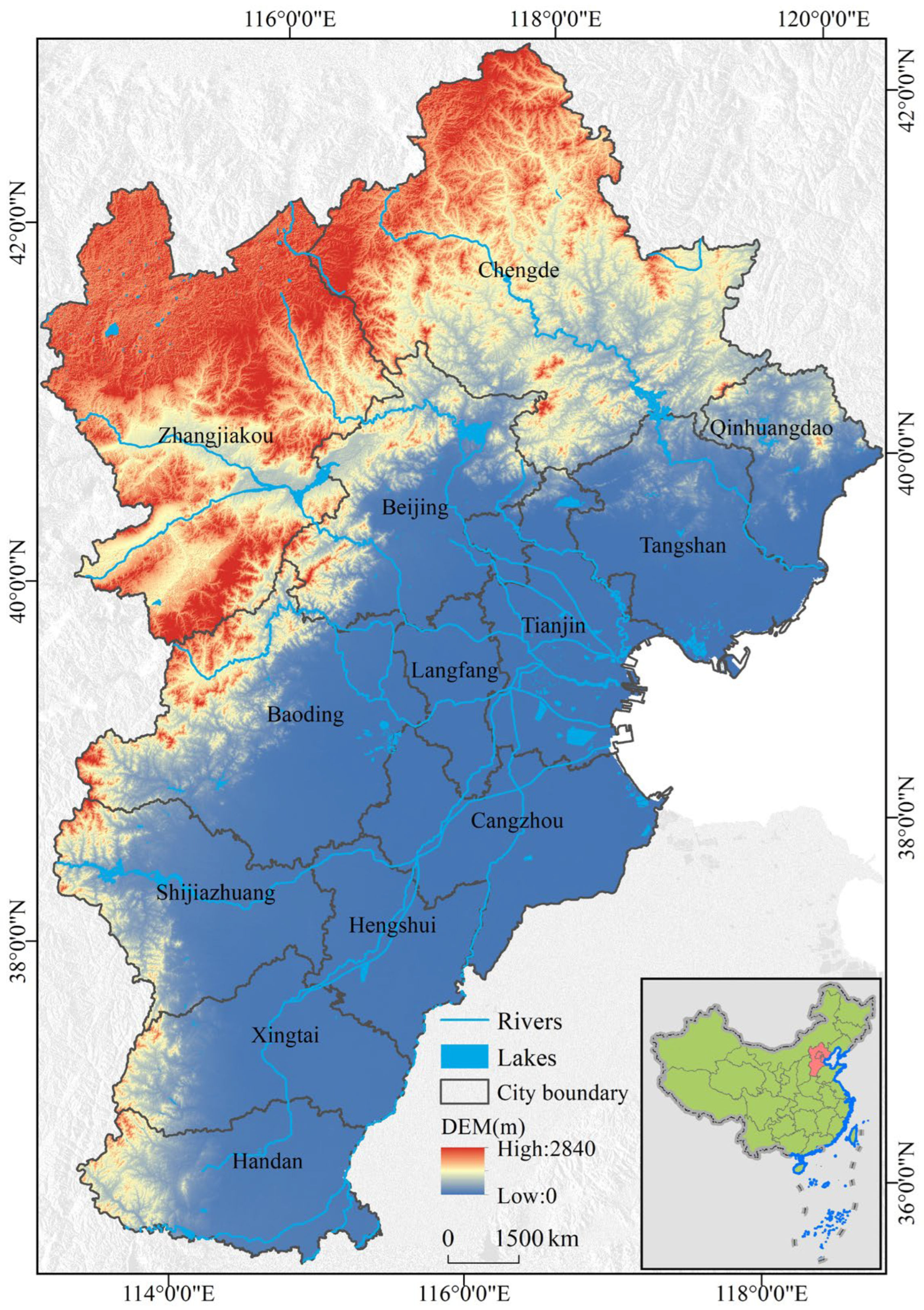
2.1. Study Area
2.2. Data Source
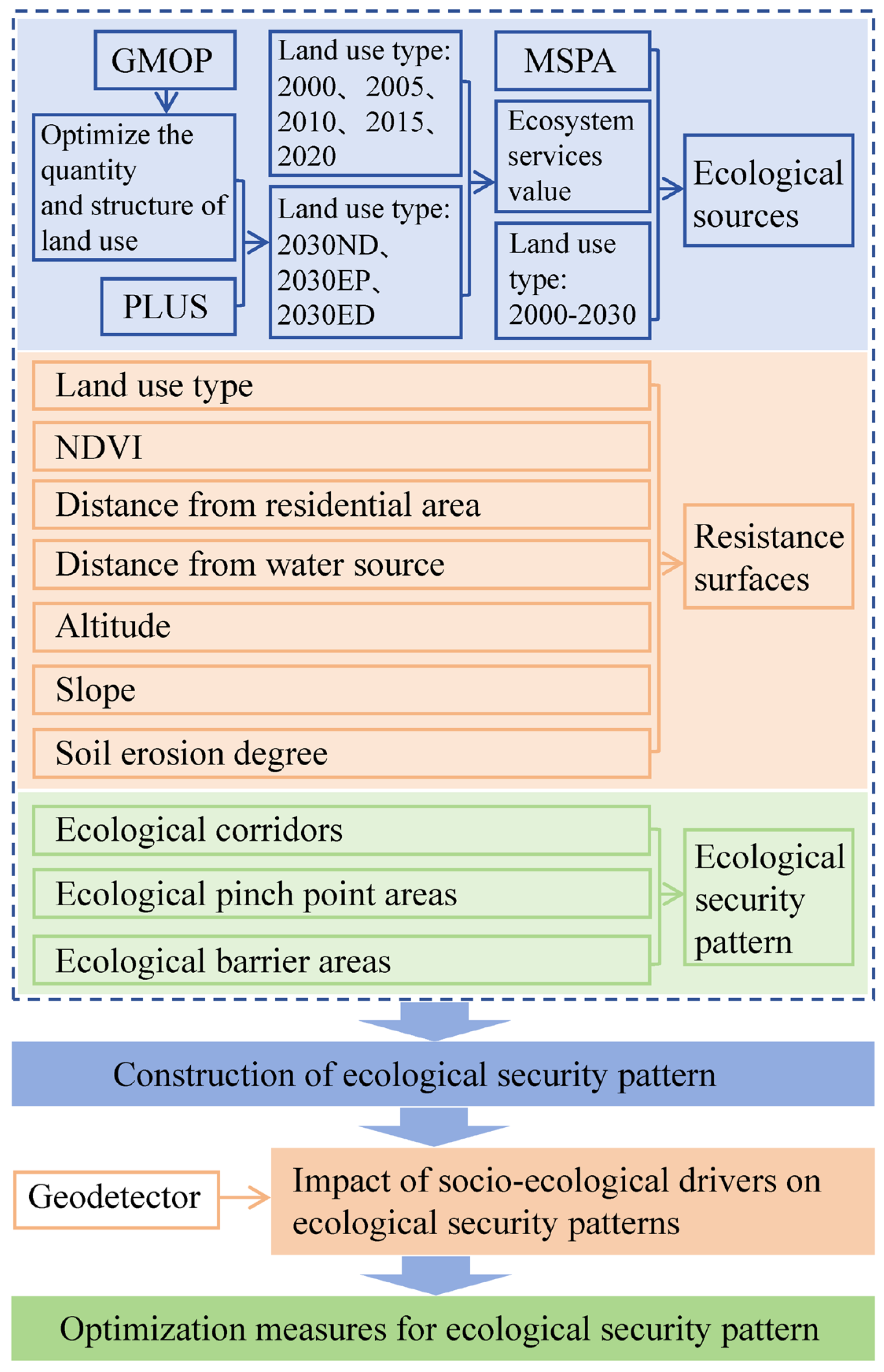
2.3. Methods
2.3.1. ESV Estimation
2.3.2. Simulation of Land Use Scenarios for 2030
2.3.3. Identifying Ecological Source Areas
2.3.4. Build Resistance Surfaces
2.3.5. Construction of the ESP
2.3.6. Stability Analysis
2.3.7. Impact of Socio-Ecological Drivers on the ESP
3. Results
3.1. Analysis of Spatiotemporal Changes in Ecological Sources
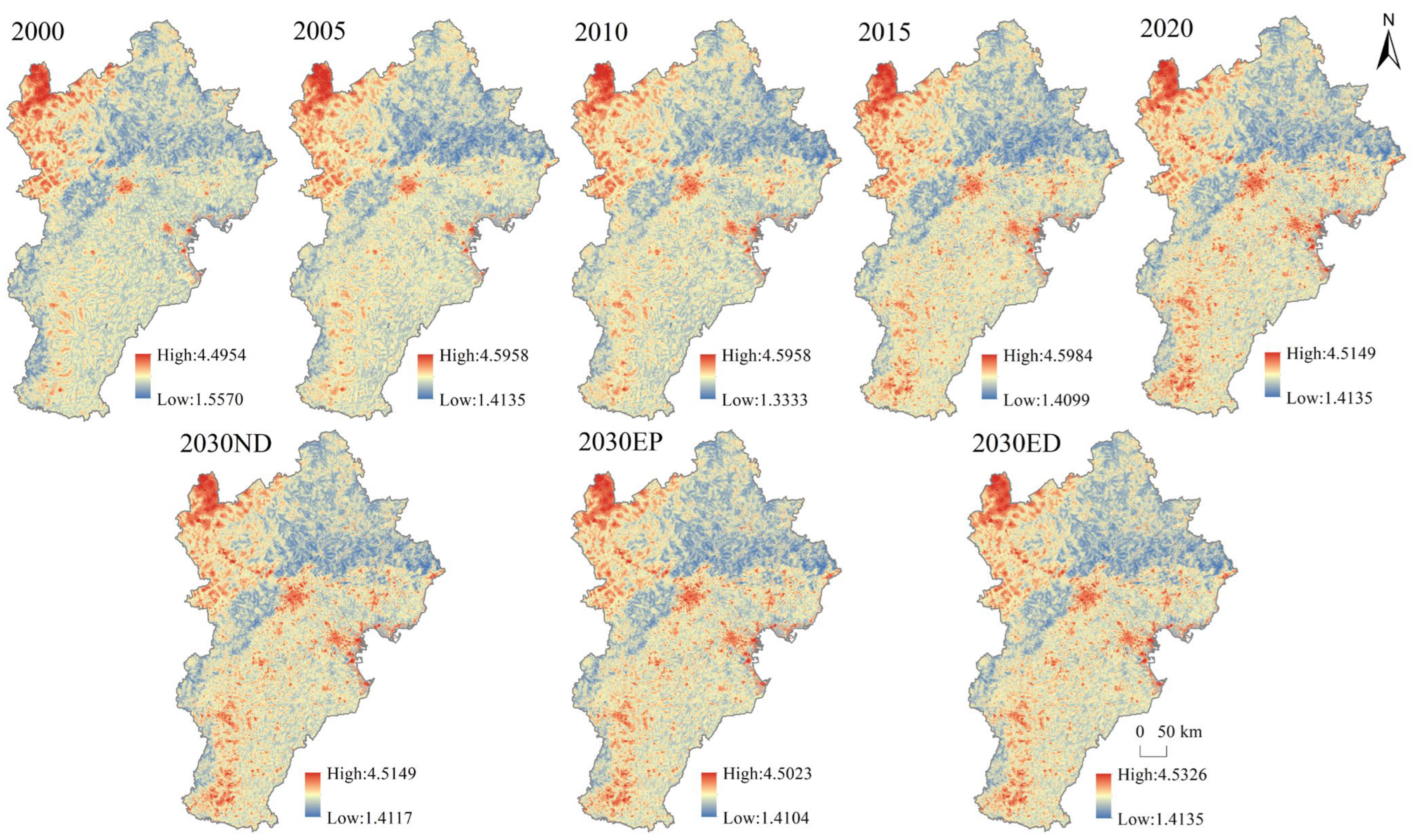
3.2. Analysis of Spatiotemporal Changes in Ecological Resistance Surfaces
3.3. Analysis of Spatiotemporal Changes in Ecological Corridors
3.4. Analysis of Spatiotemporal Changes in Ecological Pinch Point Areas
3.5. Analysis of Spatiotemporal Changes in Ecological Barrier Areas
3.6. Coefficient of Variation of ESP Components
3.7. Analysis of Spatiotemporal Changes in ESP
3.8. Socio-Ecological Drivers of the ESP
4. Discussion
4.1. Identifying the ESP
4.2. Drivers of the ESP
4.3. Prediction in 2030
4.4. ESP in the Same or Different Regions
4.5. Recommendations
4.6. Limitations and Prospects
5. Conclusions
- (1)
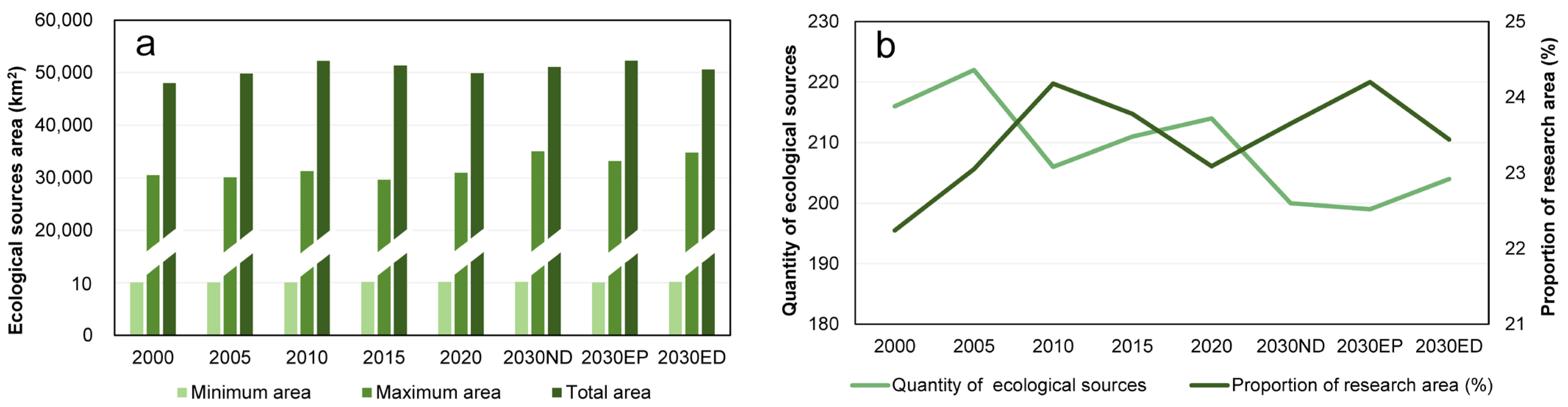
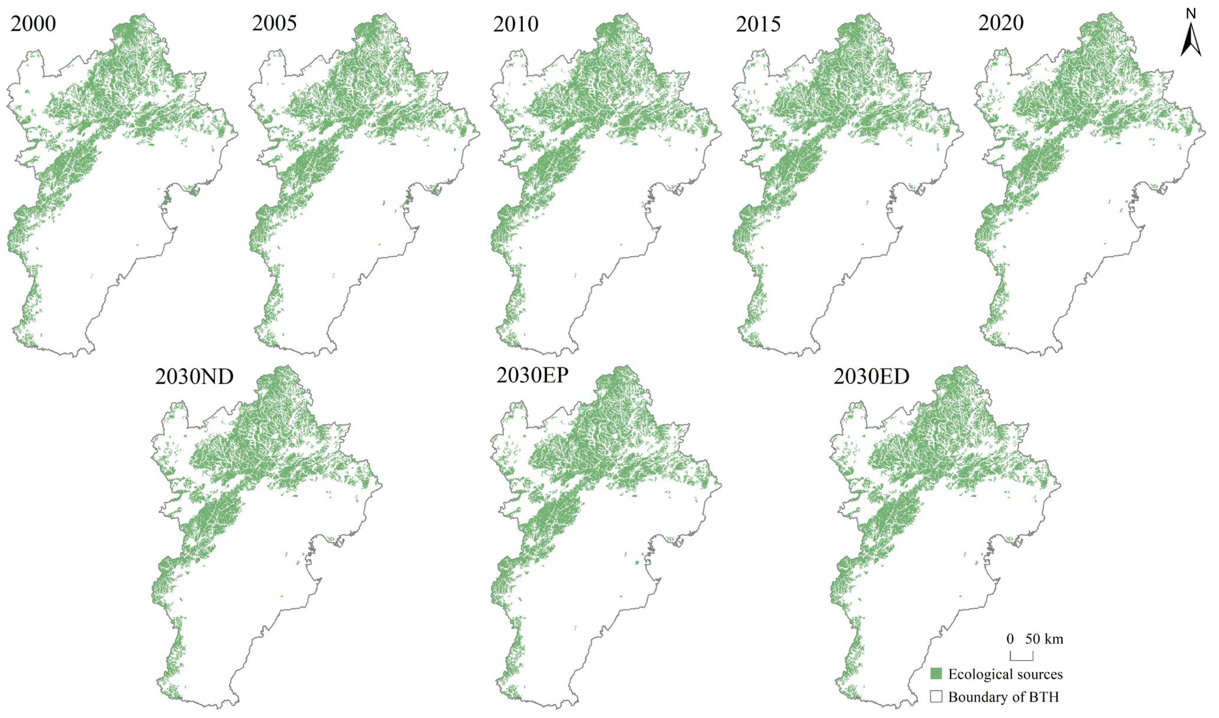
- The proportion of ecological source areas in BTH increased from 22.24% in 2000 to 23.09% in 2020. By 2030, under the EP scenario, the proportion of ecological source areas was predicted to reach the highest at 24.20%, with dense distributions in the western and northern mountainous areas, and sparser distributions in the northwestern Bashang area and the southern plains. The spatial extent of high-value ecological resistance areas expanded, mainly concentrating in the southern plains, with the northwestern Bashang area consistently being a high-resistance region.
- (2)
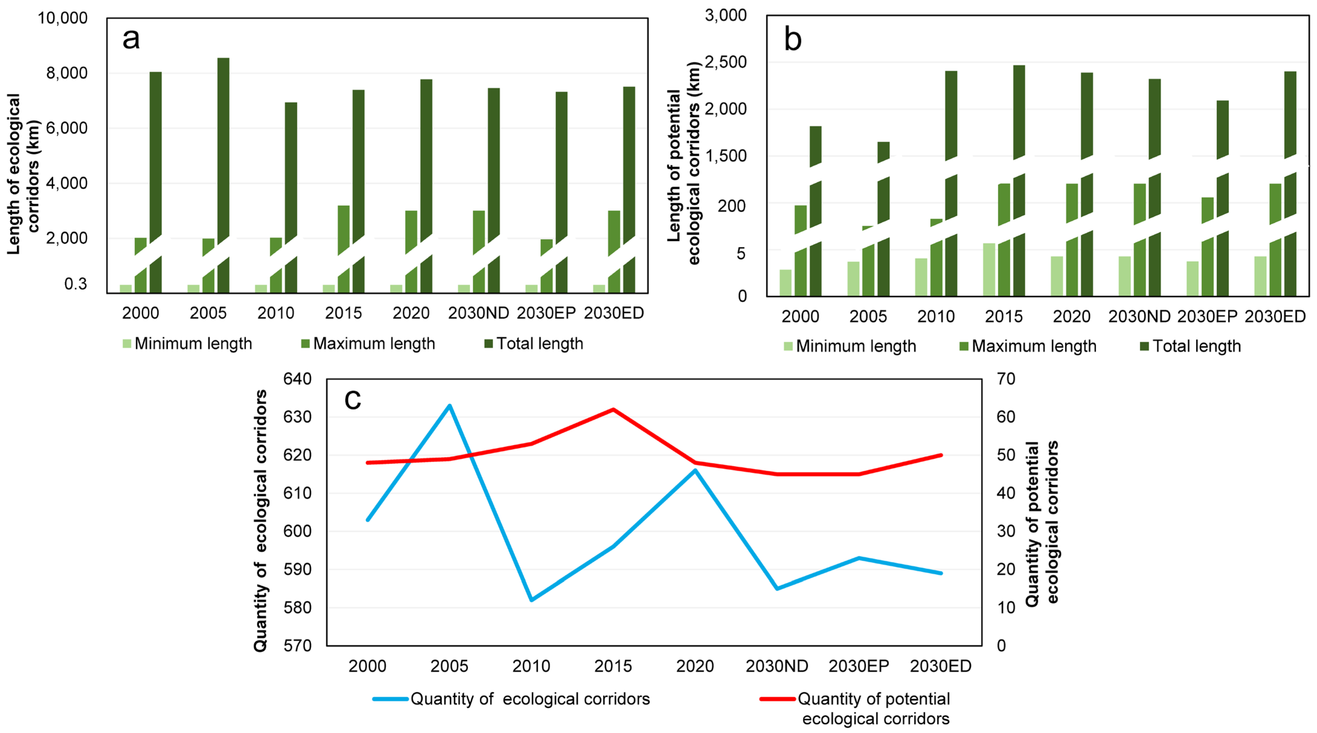
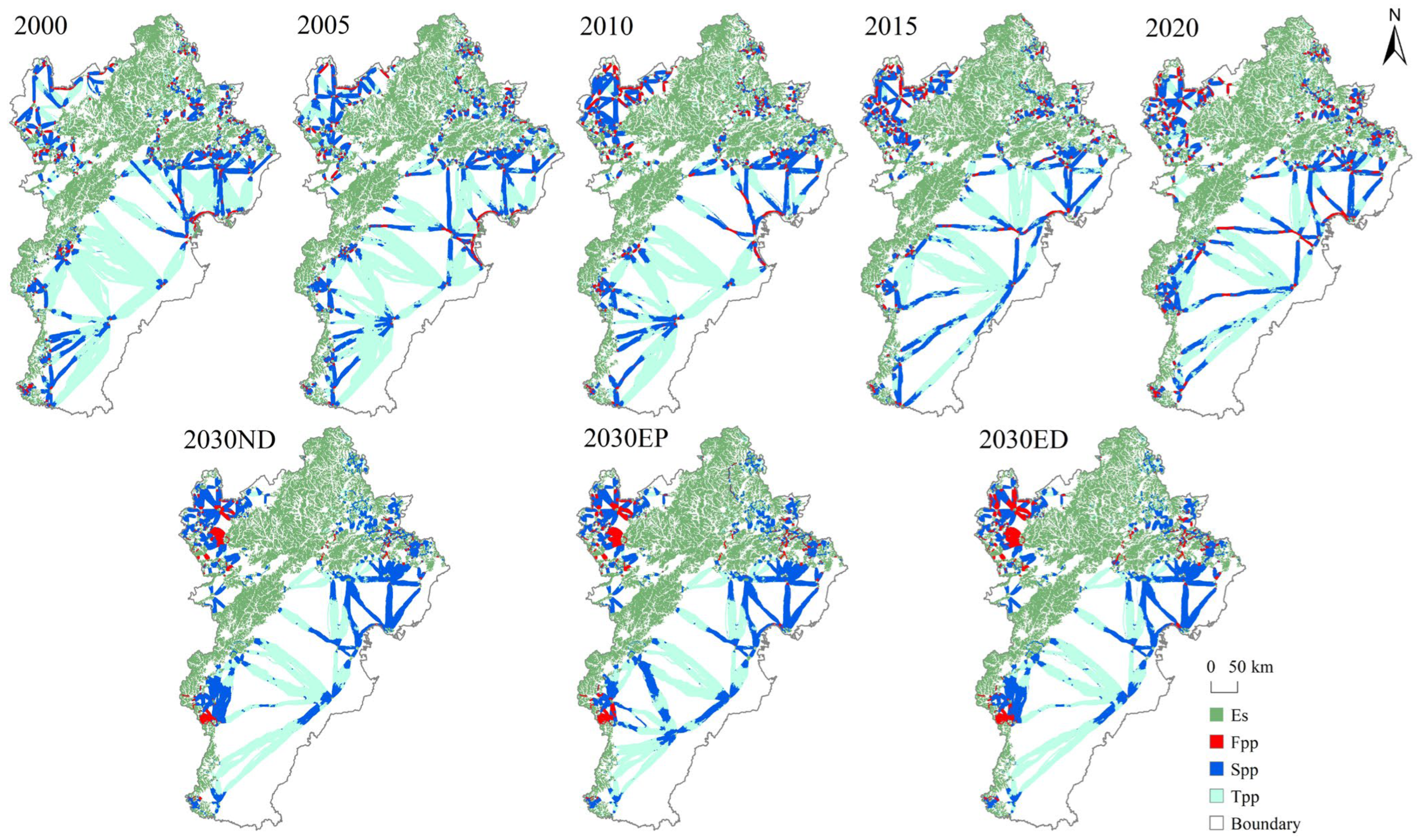
- From 2000 to 2020, the number of ecological corridors increased from 603 to 616. By 2030, the number of corridors under the EP scenario (593) was predicted to exceed those in the ND (585) and ED (589) scenarios. From 2000 to 2030, corridors in the northern and western mountains were denser, shorter, and more variable, while those in the southern plains were less dense, longer, and relatively stable.
- (3)
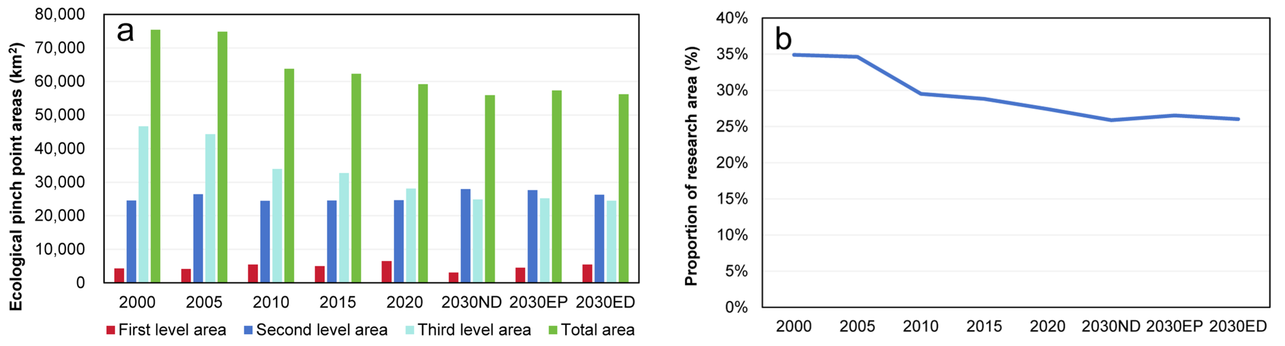
- The proportion of ecological pinch point areas decreased from 34.91% in 2000 to 27.41% in 2020. By 2030, under the EP scenario, the proportion of pinch point areas (26.53%) was predicted to be higher than in the ND (25.87%) and ED (26.01%) scenarios. From 2000 to 2030, pinch point areas were densely distributed in the northwest, northeast, and southwest, with sparse distributions in the southeast.
- (4)
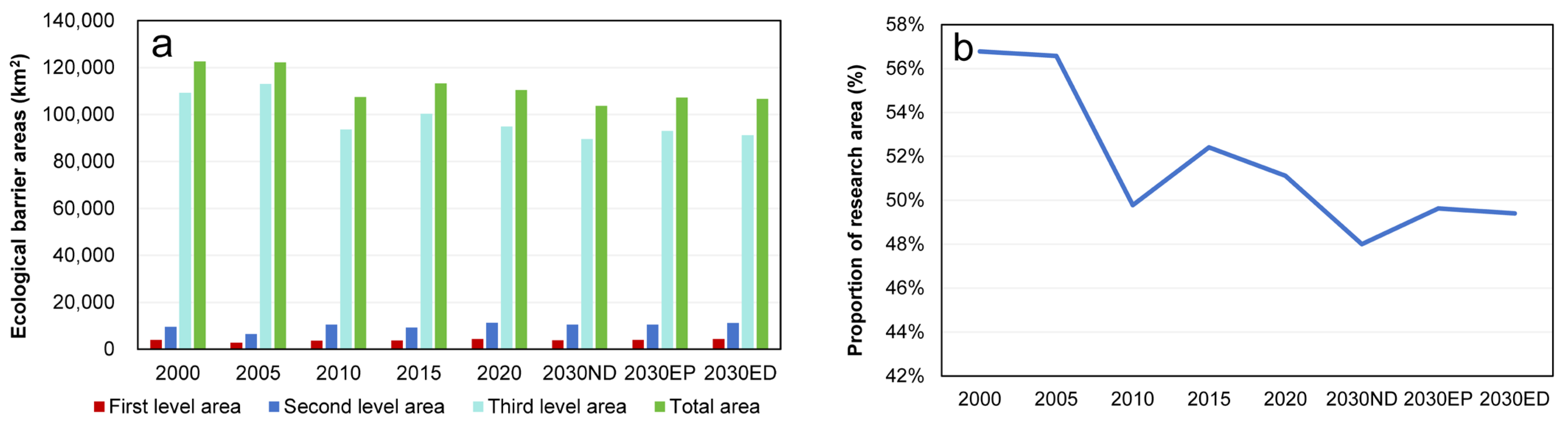
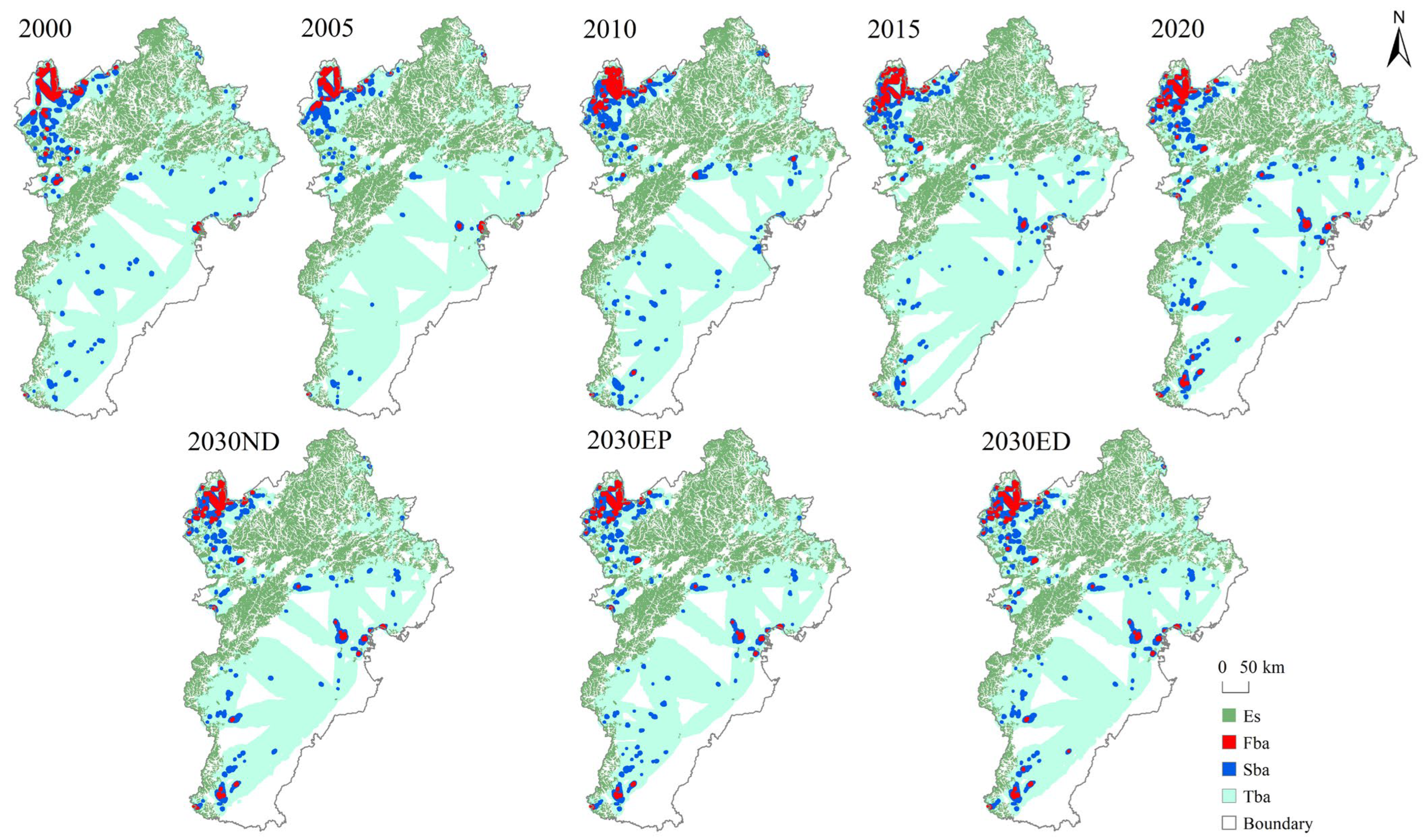
- The proportion of ecological barrier areas dropped from 56.78% in 2000 to 51.12% in 2020. By 2030, the EP scenario was predicted to have a lower proportion of barrier areas (48.00%) compared with the ND (49.63%) and ED (49.40%) scenarios. From 2000 to 2030, barrier areas were more densely distributed in the northern part of the region, with more dispersed distributions in the south.
- (5)
- From 2000 to 2020, habitat areas for species in BTH increased, while landscape connectivity decreased. By 2030, the EP scenario was predicted to have increased habitat areas and improved landscape connectivity compared with 2020 and the ND and ED scenarios, leading to some optimization of the ESP. From 2000 to 2030, the density of the ESP was greater in the north than in the south, with conservation areas mainly concentrated in the northern and western mountains, improvement areas distributed in bands across the southern plains, and restoration and key areas mainly located in Zhangjiakou city, western Chengde city, and scattered throughout the southern plains.
- (6)
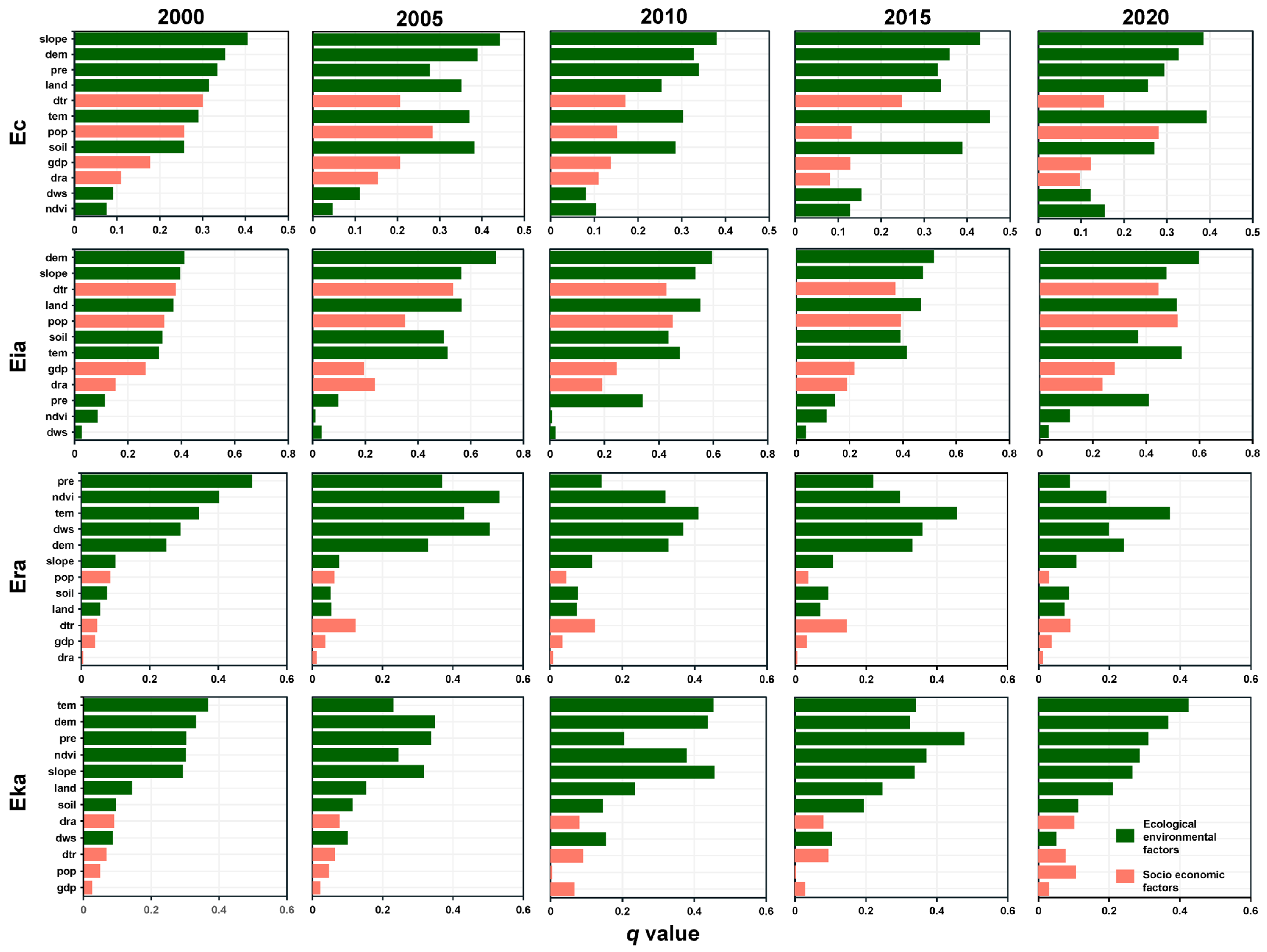
- The dominant driving factors of the ESP varied over time. The impact on ecological corridors and improvement areas mainly came from a combination of socio-ecological drivers (such as elevation, slope, distance from main transportation roads, and population), while the influence on restoration areas and key areas predominantly came from ecological environmental factors (such as elevation, temperature, NDVI, precipitation). Distinguishing different geomorphological units to improve and restore the regional environment, while considering socio-ecological drivers, is crucial for restoring the overall ESP and landscape connectivity of BTH.
Author Contributions
Funding
Data Availability Statement
Conflicts of Interest
References
- Weng, Q.; Qin, Q.; Li, L. A comprehensive evaluation paradigm for regional green development based on “five-circle model”: A case study from Beijing Tianjin-Hebei. J. Clean. Prod. 2020, 277, 124076. [Google Scholar] [CrossRef]
- Sonter, L.J.; Johnson, J.A.; Nicholson, C.C.; Richardson, L.L.; Watson, K.B.; Ricketts, T.H. Multi-site interactions: Understanding the offsite impacts of land use change on the use and supply of ecosystem services. Ecosyst. Serv. 2017, 23, 158–164. [Google Scholar] [CrossRef]
- Peters, M.K.; Hemp, A.; Appelhans, T.; Becker, J.N.; Behler, C.; Classen, A. Climate-land-use interactions shape tropical mountain biodiversity and ecosystem functions. Nature 2019, 568, 88–92. [Google Scholar] [CrossRef] [PubMed]
- Huang, L.S.; Tang, Y.; Du, Y. Ecosystem service trade-offs and synergies and their drivers in severely affected areas of the Wenchuan earthquake, China. Land Degrad. Dev. 2024, 35, 3881–3896. [Google Scholar] [CrossRef]
- Lu, Y.; Yang, J.; Peng, M.; Li, T.; Wen, D.; Huang, X. Monitoring ecosystem services in the Guangdong-Hong Kong-Macao Greater Bay Area based on multi-temporal deep learning. Sci. Total Environ. 2022, 822, 153662. [Google Scholar] [CrossRef] [PubMed]
- Xie, H.; Wen, J.; Choi, Y. How the SDGs are implemented in China-a comparative study based on the perspective of policy instruments. J. Clean. Prod. 2021, 291, 125937. [Google Scholar] [CrossRef]
- Tian, J.; Gang, G. Research on regional ecological security assessment. Energy Proc. 2012, 16, 1180–1186. [Google Scholar] [CrossRef]
- Xie, H.; He, Y.; Choi, Y.; Chen, Q.; Cheng, H. Warning of negative effects of land use changes on ecological security based on GIS. Sci. Total Environ. 2020, 704, 135427. [Google Scholar] [CrossRef]
- Ke, X.; Wang, X.; Guo, H.; Yang, C.; Zhou, Q.; Mougharbel, A. Urban ecological security evaluation and spatial correlation research-based on data analysis of 16 cities in Hubei Province of China. J. Clean. Prod. 2021, 311, 127613. [Google Scholar] [CrossRef]
- Liu, C.; Li, W.; Xu, J.; Zhou, H.; Li, C.; Wang, W. Global trends and characteristics of ecological security research in the early 21st century: A literature review and bibliometric analysis. Ecol. Indicat. 2022, 137, 108734. [Google Scholar] [CrossRef]
- Peng, J.; Yang, Y.; Liu, Y.X.; Hu, Y.N.; Du, Y.Y.; Meersmans, J.; Qiu, S.J. Linking ecosystem services and circuit theory to identify ecological security patterns. Sci. Total Environ. 2018, 644, 781–790. [Google Scholar] [CrossRef] [PubMed]
- Zhang, Z.F.; Zhao, W.; Gu, X.K. Changes resulting from a land consolidation project(LCP)and its resource environment effects: A case study in Tianmen City of Hubei Province, China. Land Use Policy 2014, 40, 74–82. [Google Scholar] [CrossRef]
- Shen, J.; Li, S.; Liu, L.; Liang, Z.; Wang, Y.; Wang, H.; Wu, S. Uncovering the relationships between ecosystem services and social-ecological drivers at different spatial scales in the Beijing-Tianjin-Hebei region. J. Clean. Prod. 2021, 290, 125193. [Google Scholar] [CrossRef]
- Hong, S.K.; Song, I.J.; Kim, H.O.; Lee, E.K. Landscape pattern and its effect on ecosystem functions in Seoul Metropolitan area: Urban ecology on distribution of the naturalized plant species. J. Environ. Sci. 2003, 15, 199–204. [Google Scholar]
- Dorner, B.; Lertzman, K.; Fall, J. Landscape pattern in topographically complex landscapes: Issues and techniques for analysis. Landsc. Ecol. 2002, 17, 729–743. [Google Scholar] [CrossRef]
- Kong, F.; Yin, H.; Nakagoshi, N.; Zong, Y. Urban green space network development for biodiversity conservation: Identification based on graph theory and gravity modeling. Landsc. Urban Plan. 2010, 95, 16.e27. [Google Scholar] [CrossRef]
- Wu, Z.H.; Lei, S.G.; Lu, Q.Q.; Bian, Z.F. Impacts of large-scale open-pit coal base on the landscape ecological health of semi-arid grasslands. Remote Sens. 2019, 11, 1820. [Google Scholar] [CrossRef]
- Qin, M.L.; Xu, H.T.; Bushman, B. The Ecological Effects of Spatial Changes in the Urban Ecological Territory. Adv. Mater. Res. 2012, 347–353, 2819–2828. [Google Scholar] [CrossRef]
- Yu, J.; Tang, B.; Chen, Y.H.; Zhang, L.; Nie, Y.; Deng, W.S. Landscape ecological risk assessment and ecological security pattern construction in landscape resource-based city: A case study of Zhangjiajie City. Acta Ecol. Sin. 2022, 42, 1290–1299. [Google Scholar]
- Li, S.C.; Wu, X.; Zhao, Y.L.; Lv, X.J. Incorporating ecological risk index in the multi-process MCRE model to optimize the ecological security pattern in a semi-arid area with intensive coal mining: A case study in northern China. J. Clean. Prod. 2020, 247, 119143. [Google Scholar] [CrossRef]
- Yang, L.A.; Li, Y.L.; Jia, L.J.; Ji, Y.F.; Hu, G.G. Ecological risk assessment and ecological security pattern optimization in the middle reaches of the Yellow River based on ERI + MCR model. Acta Geogr. Sin. 2023, 33, 22. [Google Scholar] [CrossRef]
- Mcrae, B.H.; Dickson, B.G.; Keitt, T.H.; Shah, V.B. Using circuit theory to model connectivity in ecology, evolution, and conservation. Ecology 2008, 89, 2712–2724. [Google Scholar] [CrossRef] [PubMed]
- Tang, F.; Zhou, X.; Wang, L.; Zhang, Y.; Zhang, P. Linking ecosystem service and MSPA to construct landscape ecological network of the Huaiyang section of the grand canal. Land 2021, 10, 919. [Google Scholar] [CrossRef]
- Lai, X.Y.; Yu, H.R.; Liu, G.H.; Zhang, X.X.; Feng, Y.; Ji, Y.W.; Zhao, Q.; Jiang, J.Y.; Gu, X.C. Construction and Analysis of Ecological Security Patterns in the Southern Anhui Region of China from a Circuit Theory Perspective. Remote Sens. 2023, 15, 1385. [Google Scholar] [CrossRef]
- Gao, J.B.; Du, F.J.; Zuo, L.Y.; Jiang, Y. Integrating ecosystem services and rocky desertification into identification of karst ecological security pattern. Landsc. Ecol. 2020, 36, 2113–2133. [Google Scholar] [CrossRef]
- An, Y.; Liu, S.L.; Sun, Y.X.; Shi, F.; Beazley, R. Construction and optimization of an ecological network based on morphological spatial pattern analysis and circuit theory. Landsc. Ecol. 2021, 36, 2059–2076. [Google Scholar] [CrossRef]
- Carroll, C.; Mcrae, B.H.; Brookes, A. Use of linkage mapping and centrality analysis across habitat gradients to conserve connectivity of gray wolf populations in western North America. Conserv. Biol. 2012, 26, 78–87. [Google Scholar] [CrossRef]
- Huang, J.M.; Hu, Y.C.; Zheng, F.Y. Research on recognition and protection of ecological security patterns based on circuit theory: A case study of Jinan City. Environ. Sci. Pollut. Res. 2020, 27, 12414–12427. [Google Scholar] [CrossRef]
- Wei, B.H.; Kasimu, A.; Fang, C.L.; Reheman, R.; Zhang, X.L.; Han, F.Q.; Zhao, Y.Y.; Aizizia, Y. Establishing and optimizing the ecological security pattern of the urban agglomeration in arid regions of China. J. Clean. Prod. 2023, 427, 139301. [Google Scholar] [CrossRef]
- Yan, M.M.; Duan, J.L.; Li, Y.B.; Yu, Y.; Wang, Y.; Zhang, J.W.; Qiu, Y. Construction of the Ecological Security Pattern in Xishuangbanna Tropical Rainforest Based on Circuit Theory. Sustainability 2024, 16, 3290. [Google Scholar] [CrossRef]
- Xiang, A.M.; Yue, Q.F.; Zhao, X.Q. Identification and restoration zoning of key areas for ecological restoration of territorial space in southwestern karst mountainous areas: A case study of Kaiyuan City in karst mountainous area of Southwest China. China Environ. Sci. 2023, 43, 6571–6582. [Google Scholar]
- Yu, W.; Zhang, D.; Liao, J.; Ma, L.; Zhu, X.; Zhang, W.; Hu, W.; Ma, Z.; Chen, B. Linking ecosystem services to a coastal bay ecosystem health assessment: A comparative case study between Jiaozhou Bay and Daya bay, China. Ecol. Indic. 2022, 135, 108530. [Google Scholar] [CrossRef]
- Li, Z.X.; Chang, J.; Li, C.; Gu, S.H. Ecological Restoration and Protection of National Land Space in Coal Resource-Based Cities from the Perspective of Ecological Security Pattern: A Case Study in Huaibei City, China. Land 2023, 12, 442. [Google Scholar] [CrossRef]
- Jiang, H.; Peng, J.; Liu, M.L.; Dong, J.Q.; Ma, C.H. Integrating patch stability and network connectivity to optimize ecological security pattern. Landsc. Ecol. 2024, 39, 54. [Google Scholar] [CrossRef]
- Kim, J.; Song, Y. Integrating ecosystem services and ecological connectivity to prioritize spatial conservation on Jeju Island, South Korea. Landsc. Urban Plan. 2023, 239, 104865. [Google Scholar] [CrossRef]
- Wang, Y.S.; Zhang, F.; Li, X.Y.; Johnson, V.C.; Tan, M.L.; Kung, H.; Shi, J.C.; Bahtebay, J.; He, X. Methodology for Mapping the Ecological Security Pattern and Ecological Network in the Arid Region of Xinjiang, China. Remote Sens. 2023, 15, 2836. [Google Scholar] [CrossRef]
- Kan, H.; Ding, G.Q.; Guo, J.; Liu, J.; Ou, M.H. Identification of key areas for ecological restoration of territorial space based on ecological security pattern analysis: A case study of the Taihu Lake city cluster. Chin. J. Appl. Ecol. 2024, 11, 1301149. [Google Scholar] [CrossRef]
- Jia, Q.Q.; Jia, L.M.; Lian, X.H.; Wang, W.L. Linking supply-demand balance of ecosystem services to identify ecological security patterns in urban agglomerations. Sustain. Cities Soc. 2023, 92, 104497. [Google Scholar] [CrossRef]
- Jiang, H.; Peng, J.; Dong, J.; Zhang, Z.; Xu, Z.; Meersmans, J. Linking ecological background and demand to identify ecological security patterns across the Guangdong-Hong Kong-Macao Greater Bay Area in China. Landsc. Ecol. 2021, 36, 2135–2150. [Google Scholar] [CrossRef]
- Li, W.J.; Kang, J.W.; Wang, Y. Spatiotemporal changes and driving forces of ecological security in the Chengdu-Chongqing urban agglomeration, China: Quantification using health-services-risk framework. J. Clean. Prod. 2023, 389, 136135. [Google Scholar] [CrossRef]
- Fu, Y.Y.; Zhang, W.J.; Gao, F.; Bi, X.; Wang, P.; Wang, X.J. Ecological Security Pattern Construction in Loess Plateau Areas—A Case Study of Shanxi Province, China. Land 2024, 13, 709. [Google Scholar] [CrossRef]
- Liu, H.L.; Wang, Z.L.; Zhang, L.P.; Tang, F.; Wang, G.Y.; Li, M. Construction of an ecological security network in the Fenhe River Basin and its temporal and spatial evolution characteristics. J. Clean. Prod. 2023, 417, 137961. [Google Scholar] [CrossRef]
- Xu, X.B.; Yang, G.S.; Tan, Y. Identifying ecological red lines in China’s Yangtze River Economic Belt: A regional approach. Ecol. Indic. 2019, 96, 635–646. [Google Scholar] [CrossRef]
- Terrado, M.; Sabater, S.; Chaplin-Kramer, B.; Mandle, L.; Ziv, G.; Acuña, V. Model development for the assessment of terrestrial and aquatic habitat quality in conservation planning. Sci. Total Environ. 2016, 540, 63–70. [Google Scholar] [CrossRef] [PubMed]
- Luo, J.; Zhan, J.Y.; Lin, Y.Z.; Zhao, C.H. An equilibrium analysis of the land use structure in the Yunnan Province, China. Front. Earth Sci. 2014, 8, 393–404. [Google Scholar] [CrossRef]
- Kang, J.F.; Fang, L.; Li, S.; Wang, X.R. Parallel cellular automata Markov model for land use change prediction over Mapreduce framework. ISPRS Int. J. Geo-Inf. 2019, 8, 454. [Google Scholar] [CrossRef]
- Zhou, X.Y. Spatial explicit management for the water sustainability of coupled human and natural systems. Environ. Pollut. 2019, 251, 292–301. [Google Scholar] [CrossRef]
- Luo, G.; Yin, C.; Chen, X. Combining system dynamic model and CLUE-S model to improve land use scenario analyses at regional scale: A case study of Sangong watershed in Xinjiang, China. Ecol. Complex. 2010, 7, 198–207. [Google Scholar] [CrossRef]
- Hamad, R.; Balzter, H.; Kolo, K. Predicting Land Use/Land Cover Changes Using a CA-Markov Model under Two Different Scenarios. Sustainability 2018, 10, 3421. [Google Scholar] [CrossRef]
- Zhang, Z.X.; Wei, Y.Z.; Li, X.T.; Wan, D.; Shi, Z.W. Study on Tianjin Land-Cover Dynamic Changes, Driving Factor Analysis, and Forecasting. Land 2024, 13, 726. [Google Scholar] [CrossRef]
- Dong, K.N.; Wang, H.W.; Luo, K.; Yan, X.M.; Yi, S.Y.; Huang, X. The Use of an Optimized Grey Multi-Objective Programming-PLUS Model for Multi-Scenario Simulation of Land Use in the Weigan-Kuche River Oasis, China. Land 2024, 13, 802. [Google Scholar] [CrossRef]
- Liang, X.; Guan, Q.F.; Clarke, K.C.; Liu, S.S.; Wang, B.Y.; Yao, Y. Understanding the drivers of sustainable land expansion using a patch-generating land use simulation (PLUS) model: A case study in Wuhan, China. Comput. Environ. Urban Syst. 2021, 85, 101569. [Google Scholar] [CrossRef]
- Liang, X.; Liu, X.P.; Li, D.; Zhao, H.; Chen, G.Z. Urban growth simulation by incorporating planning policies into a CA-based future land-use simulation model. Int. J. Geogr. Inf. Sci. 2018, 32, 2294–2316. [Google Scholar] [CrossRef]
- Wang, H.; Bao, C. Scenario modeling of ecological security index using system dynamics in Beijing-Tianjin-Hebei urban agglomeration. Ecol. Indic. 2021, 125, 107613. [Google Scholar] [CrossRef]
- Zhang, Y.; Lu, X.; Liu, B.; Wu, D. Impacts of Urbanization and Associated Factors on Ecosystem Services in the Beijing-Tianjin-Hebei Urban Agglomeration, China: Implications for Land Use Policy. Sustainability 2018, 10, 4334. [Google Scholar] [CrossRef]
- Chu, X.; Deng, X.; Jin, G.; Wang, Z.; Li, Z. Ecological security assessment based on ecological footprint approach in Beijing-Tianjin-Hebei region, China. Phys. Chem. Earth 2017, 101, 43–51. [Google Scholar] [CrossRef]
- Zhang, X.; Cui, J.T.; Liu, Y.Q.; Wang, L. Geo-cognitive computing method for identifying “source-sink” landscape patterns of river basin non-point source pollution. Int. J. Agric. Biol. Eng. 2017, 10, 55–68. [Google Scholar]
- Ren, Y.F.; Fang, C.L.; Lin, X.Q. Evaluation of eco-efficiency of four major urban agglomerations in eastern coastal area of China. J. Geogr. Sci. 2017, 72, 1315–1330. [Google Scholar]
- Shen, J.; Li, S.; Liang, Z.; Liu, L.; Wu, S. Exploring the heterogeneity and nonlinearity of trade-offs and synergies among ecosystem services bundles in the Beijing-Tianjin-Hebei urban agglomeration. Ecosyst. Serv. 2020, 43, 101103. [Google Scholar] [CrossRef]
- Xie, G.D.; Zhang, C.X.; Zhang, L.M.; Chen, W.H.; Li, S.M. Improvement of the Evaluation Method for Ecosystem Service Value Based on Per Unit Area. J. Nat. Resour. 2015, 30, 1243–1254. [Google Scholar]
- Li, X.M.; Liu, Q.; Han, J.; Yuan, P.; Li, Y.M. Analysis of the Spatio-temporal Evolution of Land Intensive Use and Land Ecological Security in Tianjin from 1980 to 2019. J. Resour. Ecol. 2021, 12, 367–375. [Google Scholar]
- Chen, T.T.; Peng, L.; Wang, Q. Scenario decision of ecological security based on the trade-off among ecosystem services. China Environ. Sci. 2021, 41, 3956–3968. [Google Scholar]
- Chen, L.D.; Fu, B.J.; Zhao, W.W. Source-sink landscape theory and its ecological significance. Front. Biol. China 2008, 3, 131–136. [Google Scholar] [CrossRef]
- Peng, J.; Li, H.; Liu, Y.; Hu, Y.; Yang, Y. Identiffcation and optimization of ecological security pattern in Xiong’an New Area. Acta Geogr. Sin. 2018, 73, 701–710. [Google Scholar]
- Zhang, L.; Peng, J.; Liu, Y.X.; Wu, J.S. Coupling ecosystem services supply and human ecological demand to identify landscape ecological security pattern: A case study in Beijing–Tianjin–Hebei region, China. Urban Ecosyst. 2017, 20, 701–714. [Google Scholar] [CrossRef]
- Zhu, Q.; Yuan, Q.; Yu, D.; Zhou, W.; Zhou, L.; Han, Y.; Qi, L. Construction of ecological security network of Nor-theast China Forest Belt based on circuit theory. Chin. J. Ecol. 2021, 40, 3463–3473. [Google Scholar]
- Wang, Y.Y.; Shen, C.Z.; Jin, X.B.; Bao, G.Y.; Liu, J.; Zhou, Y.K. Developing and optimizing ecological networks based on MSPA and MCR model. Ecol. Sci. 2019, 38, 138–145. [Google Scholar]
- Zhang, X.; Wei, W.; Xie, B.; Guo, Z.; Zhou, J. Ecological carrying capacity monitoring and security pattern construction in Arid Areas of Northwest China. J. Nat. Resour. 2019, 34, 2389–2402. [Google Scholar]
- Pan, J.; Wang, Y. Ecological security evaluation and ecological pattern optimization in Taolai River Basin based on CVOR and circuit theory. Acta Ecol. Sin. 2021, 41, 2582–2595. [Google Scholar]
- Liu, Y.Y.; Zhang, Z.Y.; Tong, L.J.; Khalifa, M.; Wang, Q.; Gang, C.C.; Wang, C.Q.; Li, J.L.; Sun, Z.G. Assessing the effects of climate variation and human activities on grassland degradation and restoration across the globe. Ecol. Indic. 2019, 106, 105504. [Google Scholar] [CrossRef]
- Wang, J.F.; Zhang, T.L.; Fu, B.J. A measure of spatial stratified heterogeneity. Ecol. Indic. 2016, 67, 250–256. [Google Scholar] [CrossRef]
- Wang, J.F.; Xu, C.D. Geodetector: Principle and prospective. Acta Geogr. Sin. 2017, 72, 116–134. [Google Scholar]
- Zhang, Z.Y.; Liu, Y.F.; Wang, Y.H.; Liu, Y.F.; Zhang, Y.; Zhang, Y. What factors affect the synergy and tradeoff between ecosystem services, and how, from a geospatial perspective? J. Clean. Prod. 2020, 257, 120454. [Google Scholar] [CrossRef]
- Xue, C.L.; Chen, X.H.; Xue, L.R.; Zhang, H.Q.; Chen, J.P.; Li, D.D. Modeling the spatially heterogeneous relationships between tradeoffs and synergies among ecosystem services and potential drivers considering geographic scale in Bairin Left Banner, China. Sci. Total Environ. 2023, 855, 158834. [Google Scholar] [CrossRef]
- Wang, J.; Yan, S.C.; Guo, Y.Q.; Li, J.; Sun, G. The effects of land consolidation on the ecological connectivity based on ecosystem service value: A case study of Da’an land consolidation project in Jilin province. J. Geogr. Sci. 2015, 25, 603–616. [Google Scholar] [CrossRef]
- Peng, B.; Yang, J.C.; Li, Y.X.; Zhang, S.W. Land-Use Optimization Based on Ecological Security Pattern—A Case Study of Baicheng, Northeast China. Remote Sens. 2023, 15, 5671. [Google Scholar] [CrossRef]
- Pu, L.M.; Xia, Q. Urban Development Boundary Setting Versus Ecological Security and Internal Urban Demand: Evidence from Haikou, China. Land 2023, 12, 2018. [Google Scholar] [CrossRef]
- Xu, S.; Wang, H.; Kong, W.D. Study on Mountainous Optimization of Ecological Security Pattern Based on MCR Model from the Perspective of Disaster Prevention: A Case Study of Beijing-Tianjin-Hebei Mountainous Area. J. Catastrophol. 2021, 36, 118–123. [Google Scholar]
- Hu, Q.H.; Cong, N.; Yin, G.D. Ecological security pattern construction in typical ecological shelter zone: A case study of Chengde. Chin. J. Ecol. 2021, 40, 2914–2926. [Google Scholar]
- Zhang, Q.S.; Li, F.X.; Wang, D.W.; Li, M.C.; Chen, D. Analysis on changes of ecological spatial connectivity in Jiangsu Province based on ecological network. Acta Ecol. Sin. 2021, 41, 3007–3020. [Google Scholar]
- Xu, H.C.; Li, C.L.; Wang, H.; Liu, M.; Hu, Y.M. Impact of land use change on the spatiotemporal evolution of the regional thermal environment in the Beijing-Tianjin-Hebei urban agglomeration. China Environ. Sci. 2023, 43, 1340–1348. [Google Scholar]
- Kuang, W.H.; Yang, T.R.; Yan, F.Q. Regional urban land-cover characteristics and ecological regulation during the construction of Xiong’an New District, Hebei Province, China. Acta Geogr. Sin. 2017, 72, 947–959. [Google Scholar]
- Wang, S.; Li, W.J.; Qing Li, Q.; Wang, J.F. Ecological Security Pattern Construction in Beijing-Tianjin-Hebei Region Based on Hotspots of Multiple Ecosystem Services. Sustainability 2022, 14, 699. [Google Scholar] [CrossRef]
- Hu, B.X.; Wang, D.C.; Wang, Z.H.; Wang, F.C.; Liu, J.Y.; Sun, Z.C.; Chen, J.H. Development and optimization of the ecological network in the Beijing-Tianjin-Hebei metropolitan region. Acta Ecol. Sin. 2018, 38, 4383–4392. [Google Scholar]
- Zhang, M.N.; Xu, L.; Zhang, C.C. Study construction of ecological security pattern in Beijing-Tianjin-Hebei region and identification of early warning points. For. Ecol. Sci. 2022, 37, 408–417. [Google Scholar]
- Guo, R.; Wu, T.; Liu, M.; Huang, M.; Stendardo, L.; Zhang, Y. The Construction and Optimization of Ecological Security Pattern in the Harbin-Changchun Urban Agglomeration, China. Int. J. Environ. Res. Public Health 2019, 16, 1190. [Google Scholar] [CrossRef]
- Zhang, S.; Shao, H.; Li, X.; Xian, W.; Shao, Q.; Yin, Z.; Lai, F.; Qi, J. Spatiotemporal Dynamics of Ecological Security Pattern of Urban Agglomerations in Yangtze River Delta Based on LUCC Simulation. Remote Sens. 2022, 14, 296. [Google Scholar] [CrossRef]
- Jiao, M.Y.; Hu, M.M.; Xia, B.C. Spatiotemporal dynamic simulation of land-use and landscape-pattern in the Pearl River Delta, China. Sustain. Cities Soc. 2019, 49, 101581. [Google Scholar] [CrossRef]
- Xiao, S.C.; Wu, W.J.; Guo, J.; Ou, M.H.; Pueppke, S.G.; Ou, W.X.; Tao, Y. An evaluation framework for designing ecological security patterns and prioritizing ecological corridors: Application in Jiangsu Province, China. Landsc. Ecol. 2020, 35, 2517–2534. [Google Scholar] [CrossRef]
- Zoppi, C. Ecosystem Services, Green Infrastructure and Spatial Planning. Sustainability 2020, 12, 4396. [Google Scholar] [CrossRef]
- Zhang, H.B.; Yan, Q.Q.; Xie, F.F.; Ma, S.C. Evaluation and Prediction of Landscape Ecological Security Based on a CA-Markov Model in Overlapped Area of Crop and Coal Production. Land 2023, 12, 207. [Google Scholar] [CrossRef]
- Huang, Y.T.; Cao, Y.R.; Wu, J.Y. Evaluating the spatiotemporal dynamics of ecosystem service supply-demand risk from the perspective of service flow to support regional ecosystem management: A case study of yangtze river delta urban agglomeration. J. Clean. Prod. 2024, 460, 142598. [Google Scholar] [CrossRef]
- Yang, J.; Tang, Y. The increase in ecosystem services values of the sand dune succession in northeastern China. Heliyon 2019, 5, e02243. [Google Scholar] [CrossRef] [PubMed]
- Peng, J.; Liu, Y.X.; Wu, J.S.; Lv, H.L.; Hu, X.X. Linking ecosystem services and landscape patterns to assess urban ecosystem health: A case study in Shenzhen City, China. Landsc. Urban Plan. 2015, 143, 56–68. [Google Scholar] [CrossRef]
- Gantumur, B.; Wu, F.L.; Vandansambuu, B.; Tsegmid, B.; Dalaibaatar, E.; Zhao, Y. Spatiotemporal dynamics of urban expansion and its simulation using CA-ANN model in Ulaanbaatar, Mongolia. Geocarto Int. 2022, 37, 494–509. [Google Scholar] [CrossRef]


| Data Type | Indicators | Temporal Coverage | Spatial Resolution | Data Source |
|---|---|---|---|---|
| Land use | —— | 2000, 2005, 2010, 2015, 2020 | 30 m | http://www.resdc.cn (accessed on 10 May 2023) |
| Climate and environment | DEM | 2009 | 30 m | http://www.gscloud.cn (accessed on 8 May 2023) |
| Slope | —— | 30 m | Converted from DEM data in ArcGIS 10.5 | |
| Precipitation | 2010, 2020 | 1 km | http://www.resdc.cn (accessed on 29 June 2023) | |
| Temperature | 2010, 2020 | 1 km | http://www.resdc.cn (accessed on 29 June 2023) | |
| Soil types | 1995 | 1:1 million | http://www.resdc.cn (accessed on 29 June 2023) | |
| River system | 2020 | 1:1 million | http://www.webmap.cn (accessed on 12 July 2023) | |
| Socio-economic | POP | 2010, 2020 | 1 km | http://www.resdc.cn (accessed on 29 June 2023) |
| GDP | 2010, 2020 | 1 km | http://www.resdc.cn (accessed on 29 June 2023) | |
| Road network | 2020 | —— | http://www.webmap.cn (accessed on 12 July 2023) | |
| Grain sowing area and yield | 2010–2020 | —— | Statistical Yearbook of China | |
| Grain price | 2010–2020 | —— | Compilation of national agricultural cost–benefit data |
| Constraint Types | Constraints (km2) | Instructions |
|---|---|---|
| Land area (xi) | The total land use area remains unchanged in each scenario. | |
| Cultivated area (x1) | 92,372.04 ≤ x1 ≤ 94,446.99 | The cultivated land area in each scenario is based on the upper limit of the research area in 2020, and the lower limit is based on the area predicted by Markov Chain. |
| Forest area (x2) | 53,338.5 ≤ x2 ≤ 66,645.95 | During the research period, forest land showed an increasing trend, with the area of the study area in 2020 as the lower limit and the Markov Chain prediction area of 120% as the upper limit. |
| Shrub land area (x3) | 642.33 ≤ x3 ≤ 781.92 | During the research period, shrub land showed an increasing trend, with the lower limit being the area of the study area in 2020 and the upper limit being 120% of the Markov Chain predicted area. |
| Grassland area (x4) | x4 ≥ 32,045.94 | The grassland area in each scenario shall not be lower than the current value. |
| Water area (x5) | x5 ≥ 2852.64 | The water area in each scenario shall not be lower than the current value. |
| Wasteland area (x6) | 40.05 ≤ x6 ≤ 47.88 | As the demand for land increases, the intensity of unused land development will also increase, with the research area in 2020 as the upper limit and the Markov Chain predicted area as the lower limit. |
| Construction land area (x7) | 32,585.67 ≤ x7 ≤ 42,361.37 | Because of the development of urban construction, the construction land area is not lower than the existing area, and the increase is limited to the construction land increase indicator planned in the 2020 research area. |
| Ecological service value | ≥ 2020 | The overall ecosystem service value will be higher in 2030 than in 2020. gi: Ecological service value in different land types. |
| Economic benefit value | ≥ 2020 | The overall economic benefits in 2030 will be higher than in 2020. xi: Economic benefit value in different land types. |
| Resistance Factor | Weight | Score Assignment | ||||
|---|---|---|---|---|---|---|
| 5 | 4 | 3 | 2 | 1 | ||
| Land use type | 0.2203 | construction land, bare land | farmland | grassland | forestland, shrubbery | water body |
| NDVI | 0.1839 | <0.3 | [0.3, 0.5) | [0.5, 0.6) | [0.6, 0.8) | >0.8 |
| Distance from water source (m) | 0.1912 | >2000 | [1000, 2000) | [500, 1000) | [100, 500) | [0, 100) |
| Distance from residential area (m) | 0.1130 | [0, 200) | [200, 500) | [500, 1000) | [1000, 2000) | >2000 |
| Altitude (m) | 0.0802 | Divide into 5 categories from large to small | ||||
| Slope (°) | 0.1004 | |||||
| Soil erosion degree | 0.1110 | |||||
| Category | Indicator | Abbreviation |
|---|---|---|
| Ecological factors | Land use type | land |
| NDVI | ndvi | |
| Altitude | dem | |
| Slope | slope | |
| Soil erosion degree | soil | |
| Temperature | tem | |
| Precipitation | pre | |
| Distance from water source | dws | |
| Socio-economic factors | Distance from residential area | dra |
| Distance from main transportation roads | dtr | |
| Gross domestic product | gdp | |
| Population density | pop |
Disclaimer/Publisher’s Note: The statements, opinions and data contained in all publications are solely those of the individual author(s) and contributor(s) and not of MDPI and/or the editor(s). MDPI and/or the editor(s) disclaim responsibility for any injury to people or property resulting from any ideas, methods, instructions or products referred to in the content. |
© 2024 by the authors. Licensee MDPI, Basel, Switzerland. This article is an open access article distributed under the terms and conditions of the Creative Commons Attribution (CC BY) license (https://creativecommons.org/licenses/by/4.0/).
Share and Cite
Huang, L.; Tang, Y.; Song, Y.; Liu, J.; Shen, H.; Du, Y. Identifying and Optimizing the Ecological Security Pattern of the Beijing–Tianjin–Hebei Urban Agglomeration from 2000 to 2030. Land 2024, 13, 1115. https://doi.org/10.3390/land13081115
Huang L, Tang Y, Song Y, Liu J, Shen H, Du Y. Identifying and Optimizing the Ecological Security Pattern of the Beijing–Tianjin–Hebei Urban Agglomeration from 2000 to 2030. Land. 2024; 13(8):1115. https://doi.org/10.3390/land13081115
Chicago/Turabian StyleHuang, Longsheng, Yi Tang, Youtao Song, Jinghui Liu, Hua Shen, and Yi Du. 2024. "Identifying and Optimizing the Ecological Security Pattern of the Beijing–Tianjin–Hebei Urban Agglomeration from 2000 to 2030" Land 13, no. 8: 1115. https://doi.org/10.3390/land13081115