The Improved SBAS-InSAR Technique Reveals Three-Dimensional Glacier Collapse: A Case Study in the Qinghai–Tibet Plateau

Abstract

Many debris-covered glaciers are widely distributed on the Qinghai–Tibet Plateau. Glaciers are important freshwater resources and cause disasters such as glacier collapse and landslides. Therefore, it is of great significance to monitor the movement characteristics of large active glaciers and analyze the process of mass migration, which may cause serious threats and damage to roads and people living in surrounding areas. In this study, we chose a glacier with strong activity in Lulang County, Tibet, as the study area. The complete 4-year time series deformation of the glacier was estimated by using an improved small-baseline subset InSAR (SBAS-InSAR) technique based on the ascending and descending Sentinel-1 datasets. Then, the three-dimensional time series deformation field of the glacier was obtained by using the 3D decomposition technique. Furthermore, the three-dimensional movement of the glacier and its material migration process were analyzed. The results showed that the velocities of the Lulang glacier in horizontal and vertical directions were up to 8.0 m/year and 0.45 m/year, and these were basically consistent with the movement rate calculated from the historical optical images. Debris on both sides of the slope accumulated in the channel after slipping, and the material loss of the three provenances reached 6–9 × 10³ m³/year, while the volume of the glacier also decreased by about 76 × 10³ m³/year due to snow melting and evaporation. The correlation between the precipitation, temperature, and surface velocity suggests that glacier velocity has a clear association with them, and the activity of glaciers is linked to climate change. Therefore, in the context of global warming, the glacier movement speed will gradually increase with the annual increase in temperature, resulting in debris flow disasters in the future summer high-temperature period.

1. Introduction

The Qinghai–Tibet Plateau and its surrounding mountains have the highest concentration of glaciers at low and middle latitudes in the world, supplying water to many of Asia’s great rivers, including the Brahmaputra, Yangtze, and Indus [1]. However, it is also the cause of glacier collapse, landslides, and other disasters [2,3]. Due to the remoteness and difficulty in reaching the plateau, glacier observation data are not only scarce but also short in time [1], and sudden glacial debris flows often cause severe damage and casualties. In recent years, large glacial disasters (up to 120 million cubic meters) have been reported on the Tibetan Plateau, resulting in the death of dozens of people and hundreds of animals and causing massive property damage [4,5,6,7]. Therefore, it is necessary to study glacier variations, especially long-term activity, mass migration, and their possible disaster chains. Additionally, mountain glaciers are a sensitive indicator of climate change, and the study of the relationship between glacier activity and climate is of great significance for understanding global climate change.

Most glaciers are difficult to approach and study with regular in situ measurements [8]. At present, remote sensing techniques are mainly applied to understanding glacier activity. Although optical remote sensing is often hampered by inclement weather conditions [9], interferometric synthetic aperture radar (InSAR) has proven to be effective in identifying and monitoring the movement and migration of active glaciers, which uses radar waves to obtain surface information, regardless of inclement weather conditions such as clouds and rain [10,11]. Nevertheless, glaciers cannot be monitored with traditional synthetic aperture radar differential interferometry, as this technique has limitations related to the loss of coherence and the maximum observable displacement gradient/rate [12], and glacier migration is a three-dimensional movement of time series, which requires us not only to obtain the time series deformation but also to solve the three-dimensional deformation. In order to overcome these limitations, an improved small-baseline subset SBAS-InSAR technique is applied to acquire with a time span of 4 years between October 2017 and August 2021. The baseline-combination method is a method that is capable of eliminating the effect of an inaccurate digital elevation model (DEM) on the estimation of ice velocities [13], and the phase error can be reduced by combining appropriate baselines [14,15]. Compared with the original SBAS-InSAR method, the improved method uses a reasonable and dense temporal baseline and average rate interpolation method to obtain the complete time series deformation field, which effectively solves the problem that deformation cannot be obtained in a low coherence period. The three-dimensional time series deformation field of glaciers can then be solved using the time series deformation in two directions, which helps us better understand the movement and material migration process of the Lulang glacier.

In this study, we derived complete three-dimensional time series glacier velocities with strong activity and dangerousness for the Lulang area by integrating improved SBAS-InSAR and three-dimensional decomposition methods with Sentinel-1 imagery acquired on ascending and descending orbits. Then, we analyzed the mass migration process of glaciers in the past four years, revealing the current development stage and future development trend of glaciers through the three-dimensional time series movement of Lulang glaciers. The relationship between temporal deformation characteristics and climate change was further revealed, verifying the role of global climate change in catastrophic glacier disasters.

This paper is organized as follows: In Section 2, we introduce the study area and datasets used in this paper. We introduce the principle, fusion, and improved SBSA-InSAR and three-dimensional decomposition techniques in Section 3. In Section 4, the three-dimensional velocity and mass motion of glaciers are estimated, and the relationship between glacier activity and climate change is discussed. Lastly, this paper is discussed and concluded in Section 5 and Section 6.

2. Study Area and Datasets

2.1. Study Area

The study area (29.8~29.9° N, 94.78~94.86° E, Figure 1) is located on the west side of the eastern Himalayas structural junction and belongs to the alpine canyon landform in southeastern Tibet. The mountain trend is mainly south–north with a deep-cut valley; the area is 2600–6800 m above sea level, and the relative height difference between the valley bottom and the mountain top is 4200 m. The mountain is covered with snow all the year-round and has obvious features of the glacier’s landforms. Affected by the Indian Ocean warm current, the study area belongs to the plateau ocean climate and the continental climate. The annual average temperature is 2°, the highest is 18°, and the lowest is −11°. The annual temperature difference is small, but the daily temperature difference is large. Rainfall in May–September accounts for about 85% of the whole year. The Lulang glacier is located in a high mountain valley, with an average elevation of 4400 m, an average length of about 7 km, and a glacier area of about 8.5 km². The ridge and the steeply dipping mountains on both sides are a continuous source of replenishment for the glacier.

2.2. Datasets

In order to obtain information on the long-term series of glacier deformation, we collected a total of 207 scenes from Sentinel-1 data (ESA, https://scihub.copernicus.eu (accessed on 15 May 2024),

Table 1. Summary of data used in this study.

Data	Resolution	Date	Number	Source
SAR: Sentinel-1	Range 2.3 m, azimuth 14 m	10.2017–08.2021	207	ESA. https://scihub.copernicus.eu, accessed on 10 February 2022.
Sentinel-2A/B	10 m (RGB)	01.01.2016–31.12.2020	5	ESA. https://scihub.copernicus.eu, accessed on 15 February 2022.
Landsat 8	15 m	01.01.2015–31.12.2020	4	USGS. https://earthexplorer.usgs.gov, accessed on 8 January 2022.
Topographic map	30 m	-		SRTM. http://gdex.cr.usgs.gov/gdex, accessed on 15 May 2024
Rainfall	10 km	01.01.2017–31.08.2021	daily	NASA. https://pmm.nasa.gov, accessed on 24 January 2022.
Temperature	1°	01.01.2017–31.08.2021	daily	National Oceanic and Atmospheric Administration (NOAA). http://gis.ncdc.noaa.gov, accessed on 24 January 2022.

and

Table 2. Detail parameters of SAR images.

SAR Data	Time Period	Number	Path	Frame	Incident	Azimuth
Sentinel-1 (Ascending)	18.10.2017–10.08.2021	110	70	1277	33.8836°	−12.71°
Sentinel-1 (Descending)	06.11.2017–05.08.2021	97	4	491	39.2036°	192.70°

) with a time span of 4 years, including 110 and 97 scenes collected for ascending and descending orbit, respectively; the pixel spacing in the LOS and azimuth directions were 2.3 m and 14 m, respectively. Data from two observation directions can help solve problems such as shadow and overlap and solve the three-dimensional deformation of glaciers. The SRTM DEM, acquired from the United States Geological Survey (USGS), provides a 30 m resolution elevation information. We also collected a total of 9 optical images, which could help us visually observe glacier movement. Temperature and rainfall changes are the most intuitive data manifestation of climate change. Daily rainfall and daily temperature data were also collected to analyze the relationship between glacier movement and climate change.

3. Methods

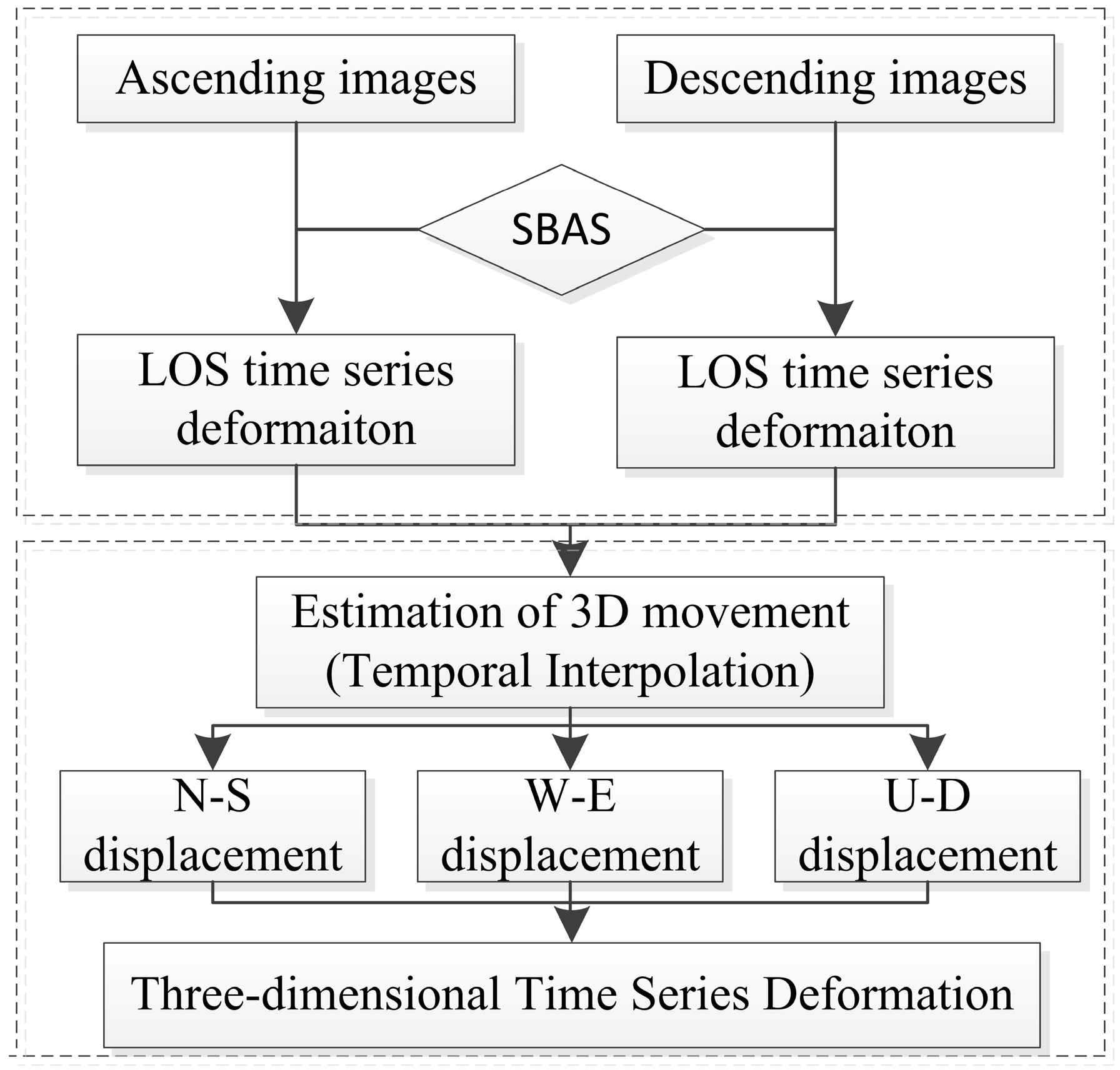
3.1. Improved SBAS-InSAR

In this paper, the improved SBAS-InSAR technique was applied to obtain time series displacement. Figure 2 shows the workflow of processing, and the detailed parameters of SAR data are shown in Table 2.

Firstly, the general processing of SBAS-InSAR began with SAR images’ co-registration [16,17], and precise orbit files were downloaded and preprocessed. After determining the interference pairs, the interferograms were generated. Then, the SRTM DEM data from the USGS were used to remove the topographic and flattened phase and geocode the InSAR products. All possible interferometric pairs interfered after co-registration and were filtered using an adaptive filtering function based on the local fringe spectrum [18] and unwrapped using the minimum cost flow (MCF) algorithm [19]. After atmospheric errors associated with elevation were removed, high-quality corrected unwrapped interferograms were selected to estimate the deformation rates and time series. Finally, the estimation of a deformation rate map was subsequently conducted using the weighted averaging of interferograms (i.e., stacking method) [20], and time series deformation, though singular value decomposition (SVD) was inversed.

Low-coherence targets such as soil in glaciers are the main factors that affect deformation information. Aiming at the acquisition of glacier deformation data in the study area, this article explains two optimizations in the original SBAS process (red words marked in Figure 2): (1) The selection of available baseline pairs was fully optimized, and two combinations of strategies were adopted (a 36-day time baseline and 180 m perpendicular baseline; three adjacent scenes’ images were combined in pairs), thereby reducing decoherence and point distortion in the time series information loss; (2) adaptive filtering and Kriging interpolation were performed on the generated interference unwrapping phase map. Adaptive filtering can reduce phase jumps and suppress noise. Kriging interpolation was used to predict and interpolate the local incoherent area of the glacier to ensure the continuity of deformation information in time. Kriging is a geostatistical forecasting method that minimizes the error variance by using a weighted linear combination of data. The weight is not only based on the distance between the measuring point and the predicted position but is also based on the overall spatial arrangement between the measuring points [21].

3.2. Three-Dimensional Decomposition

Glacier migration is a three-dimensional movement, and InSAR monitoring in a single direction makes it difficult to accurately grasp the movement situation. The three-dimensional deformation field can be derived from ascending and descending SAR images [22,23,24,25,26]. The estimated 3D displacements (du, de) can be determined from the two InSAR LOS measurements (d_los,1 and d_los,2) as follows:

$$\left[\begin{array}{c}d\mathrm{u}\\ d\mathrm{e}\end{array}\right]=\mathrm{\Gamma }\cdot \left[\begin{array}{c}{d}_{\mathrm{l}\mathrm{o}\mathrm{s},1}\\ d_{\mathrm{l}\mathrm{o}\mathrm{s},2}\end{array}\right]$$

(1)

$$\mathrm{\Gamma }=\left[\begin{array}{c}{\mathrm{\Gamma }}_1\\ {\mathrm{\Gamma }}_2\end{array}\right]={\left[\begin{array}{c}{a}_1{b}_1\\ a_2{b}_2\end{array}\right]}^{-1}$$

(2)

$$a_i=cos{\vartheta }_{\mathrm{i}\mathrm{n}\mathrm{c},\mathrm{i}},i=\mathrm{1,2}$$

(3)

$$b_i=-sin{\vartheta }_{\mathrm{i}\mathrm{n}\mathrm{c},\mathrm{i}}\sin \left({\alpha }_{\mathrm{a}\mathrm{z},\mathrm{i}}-{\displaystyle \frac{3\pi }{2}}\right),i=\mathrm{1,2}$$

(4)

$$d\mathrm{n}=\mathit{cot}{\vartheta }_{\mathrm{a}\mathrm{s}}\times d\mathrm{u}$$

(5)

where ${\vartheta }_{\mathrm{i}\mathrm{n}\mathrm{c},\mathrm{i}}$ and α_az,i are the incidence angle and orbit azimuth angle (positive clockwise from the north) for the ith InSAR LOS measurements, respectively. du and de are the vertical and east–west direction deformation; $\mathrm{\Gamma }$ is the conversion coefficient; $d_{\mathrm{l}\mathrm{o}\mathrm{s},1}$ and $d_{\mathrm{l}\mathrm{o}\mathrm{s},2}$ are the LOS deformation of ascending and descending orbits [21]; and $\mathit{cot}{\vartheta }_{\mathrm{a}\mathrm{s}}$ is the cotangent of the slope aspect. Because the N-S displacement component is extraordinarily more sensitive to the errors of the InSAR LOS measurements than the other two, we assume that the mass movement of the glacier and provenance is along the slope direction, and this is consistent with the movement of glaciers, so we can solve the N-S motion according to the solved E-W motion and slope direction. Moreover, the E-W component has the best determination, owing to the opposite imaging geometries between the ascending and descending acquisitions [24]; this makes the N-S component results have a high accuracy, as shown in Figure 3.

As the difference in acquisition dates between adjacent ascending and descending Sentinel-1 SAR data is only 5 days, it is reasonable to derive 3D time series movement by fusing ascending and descending SAR measurements [8]. Figure 4 shows the process of 3D motion component decomposition after SBAS processing and time-domain interpolation. The purpose of time-domain interpolation is to eliminate the sampling time interval between two direction orbits.

4. Results

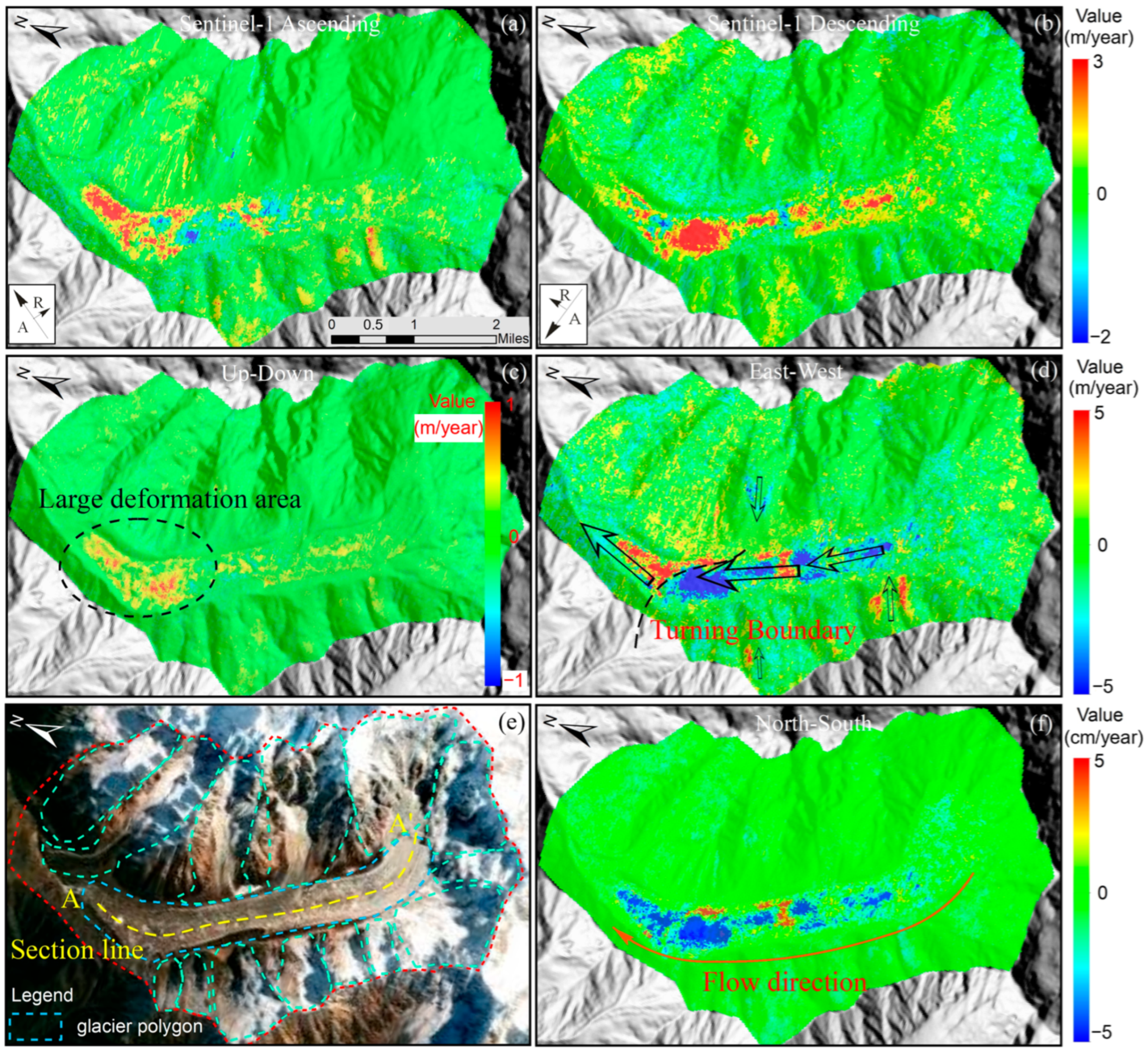
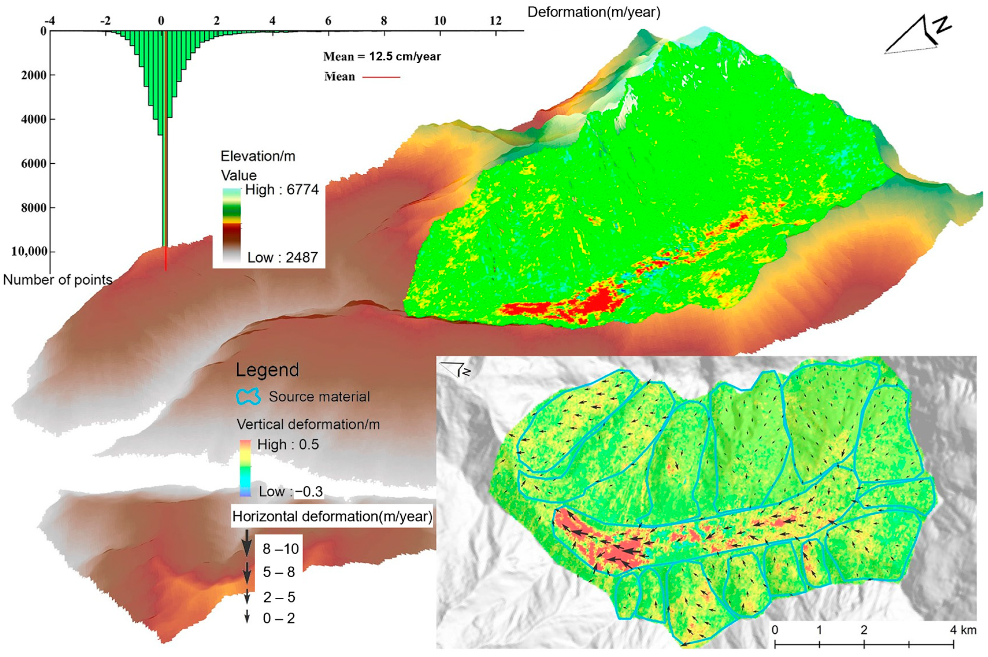
4.1. Three-Dimensional Deformation of the Glacier

Figure 5 shows the glacier LOS displacement obtained from ascending and descending Sentinel-1 SAR images and the glacier 3D displacement calculated using the method explained in Section 3.2. From the deformation observed from the two directions of ascending and descending orbits, we obtained the maximum deformation of the glacier and its steep slopes on both sides. The results in Figure 5a,b show that large deformation areas of the glacier are mainly concentrated in the front and middle parts, with LOS deformation of 1.5–2 m/year; there are also 0.5–0.8 m/year LOS deformations on the trailing edge and the steep slopes on both sides, which are the deformations caused by debris slippage on the slope. At present, there are a total of 14 small clastic areas (blue polygons in Figure 5e), which are the most important material sources of glaciers.

Figure 5c,d,f show the three-dimensional movement of the glacier. In the north–south direction, the glacier flows mostly from north to south, which is mainly controlled by the topography of the high south and low north. In general, glaciers speed up as they decrease in height, and the maximum velocity is 0.45 m/year at the front turning area (Figure 5c, marked in black dotted line), which is the area with the largest flow capacity. The material on the east and west sides of the glacier alluvialized, resulting in a small area showing a southward flow. Figure 5d shows the east–west displacement perpendicular to the movement of the glacier, which can not only indicate the boundary of the glacier east–west movement but also clearly shows the material slip characteristics of the slopes on both sides. Affected by the terrain, the direction of movement at the front of the glacier changes, and the maximum displacement in the east–west direction is about 5 m/year. The direction of movement before and after the turning is exactly in the east and west directions, so it can be clearly identified that the black dotted line and arrows in Figure 5d marked the turning boundary and the horizontal movement direction of the material. The material moving toward the gully on the slope shows that the slopes on both sides provide a constant input of material to the glacier. Through the 3D decomposition method, the true vertical displacement was obtained, as shown in Figure 5c. The maximum vertical subsidence of the glacier is 0.45 m/year, and a small part shows an uplift of 0.15 m/year, which is the accumulation area formed by the slope material after slippage. Compared with the horizontal displacement in Figure 5d–f, the vertical displacement is relatively small, which shows that the glacier mainly moves horizontally.

Through the three-dimensional terrain function of ArcScene, the complete 3D glacier velocities are shown in Figure 6. The horizontal vector was obtained by the combination of glacier deformation along the east and north, which is indicated by black arrows of different sizes. The vertical vector uses vertical displacement, which is represented by a red–green–blue color band, and the red represents settlement. As the elevation decreases, most of the glacier moves from the south to the north, and the surrounding cliffs provide a lot of material. Rugged terrain can change the moving direction, but the speed of glacier movement does not slow down significantly. The displacement histogram presents a non-standard normal distribution, and the median displacement is displayed as 12.5 cm/year, which indicates that a large number of parts in this area are in active motion.

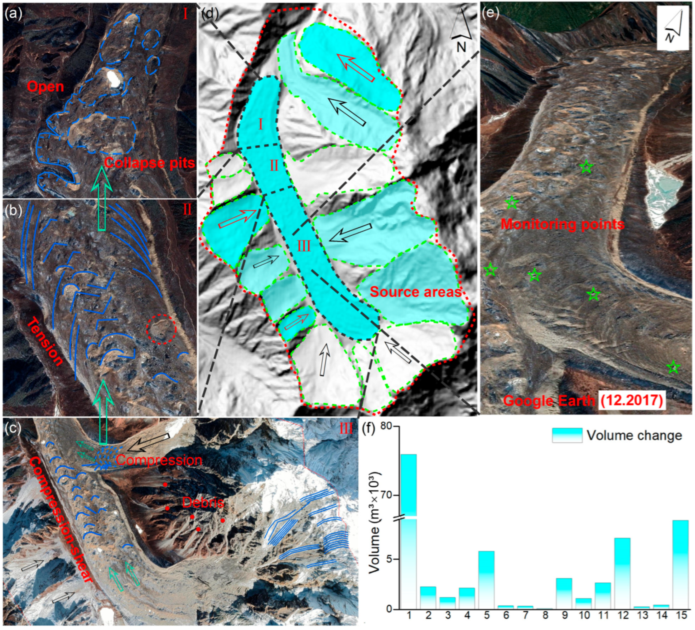
4.2. Migration Process of Glacier Material

The three-dimensional movement of glaciers derived from the improved SBAS-InSAR method can better explain the complicated migration process of glacier mass. Quantitative statistics on the displacement changes in the glacier body and the source areas on both sides can help analyze the migration process of materials. Figure 7 shows 3D velocities and elevations of glacier section line A-A’, where red, yellow, and blue colors are used to mark the three-dimensional movement rate, with positive values representing downward, north, and east displacement. The turning boundary of the glacier is about 1800 m, marked by a gray rectangular box.

The three-dimensional velocity field along the glacier section line shows that with the accumulation of material, the velocity of the glacier increases exponentially and reaches the maximum horizontal velocity 8.0 m/year (North: 5 m/year, East: 2.6 m/year) at the turning area. There are three typical zones in the process of glacier migration: energy accumulation (EA) zone, energy surge (ES) zone, and energy dissipation (ED) zone. In the EA zone, the terrain is relatively flat, and the speed of glaciers slowly increases. The material on both sides of the mountain slopes continues to gather into the main body of the glacier, causing the vertical displacement of some areas to be negative, that is, the ground is uplifted. In the ES zone, the speed of the glacier increases rapidly, and the rapid horizontal migration causes the thickness of the glacier to decrease, which is manifested as a vertical subsidence of 0.2 m/year. At the turning area, the glacier enters the ES zone. Due to the obstacles and friction generated by the mountain, the moving direction of the glacier changes. In particular, the transition of the motion vector of the glacier in the east–west direction can be accurately observed in the InSAR results. At this time, the speed of glacier movement is greatly reduced, showing a gradual decrease. The change in terrain slope is important and related to glacier movement. The terrain becomes steeper in the ES zone, and the average slope changes from 5° to 7°, which provides a lot of potential energy for glacier acceleration. After the turning area, the slope becomes 5° again, and the glacier also shows a decelerating trend.

Figure 8 shows the geomorphological characteristics and volume changes in the glacier and its provenance on both sides. Figure 8a–c are Google Earth images of local areas (EA, ES, and ED), respectively. Zone III is the area where material accumulation and the glacier start, and a large amount of debris is distributed here. Streaks were left on the trailing edge after material slippage. The flow zone of the glacier exhibits compression and slight shear mechanical properties, forming transverse ridges and C-grooves. Zone II is the fastest-moving area of the glacier. The friction and pressure between the edge of the glacier and the slope lead to a large number of arc-shaped ridges, and there are a large number of hummocks and X-grooves in the middle area, which are the results of local shearing or tension. The collapse of the internal volume caused by the rapid movement forms a collapse pit (red dashed line); after the energy dissipation from the collision with the edge and the external material supply reduces, region I shows a tendency to collapse and gradual movement. Figure 8d,f show the volume changes in the glacier; the darker the blue color, the larger the volume changes. The glacier shrinks by an average of 76 × 10³ m³/year, partly due to the ground collapse caused by the evaporation of ice, snow, and water, and partly due to the loss of material flow. Three provenance areas have large volume changes of 6–9 × 10³ m³/year, which are marked by red arrows in Figure 8d. Figure 8e shows six monitoring points mentioned in the analysis below, which are used to calculate historical migration rates.

Using Google Earth images of glaciers at different times, we can calculate the movement of a specific object, such as a rock, based on its position at different times. This is also evidence of glacial material migration, which can help us calculate the migration rate of glaciers in history. Figure 9a–e show the movement of a rock along with the glacier. The motion vectors of the rock from October 2001 to December 2017 were determined against the surrounding stable areas, and the other five rocks (Figure 8e) were also counted using the same method. As shown in Figure 9f, we calculated the movement speed “k” of six rocks and found that their movement speed remained basically stable from 2001 to 2017, with the fastest speed being 7.38 m/year and the lowest speed being 3.2 m/year. This was a very small difference from our calculation of the horizontal movement rate of the glacier, proving the accuracy of our calculation results.

4.3. Link between Time Series Glacial Movement and Climate Change

In the Qinghai–Tibet Plateau, glaciers appear to be highly sensitive to climate changes, which have profound socioeconomic and environmental consequences in South and Central Asia. However, the topic of the interaction between glaciers and climate change has not been thoroughly investigated [27]. In this article, we qualitatively analyzed the relationship between glacier activity and climate change through the time series deformation of an activity point. The factors that characterize climate change were analyzed with both temperature and rainfall. Figure 10 shows the time series deformation of an active point of the glacier, where kd, kp, and kt are the slopes of the fitted curves, representing deformation, precipitation, and temperature, respectively. Combined with the 4-year temperature and rainfall data in the area, we analyzed the relationship between glacier deformation and climate changes. The green line is the daily deformation rate of the glacier; the value above zero indicates that the glacier is in motion, and the slope of the fitted curve represents the magnitude of the acceleration. The blue and red dashed lines are the rainfall and temperature curves, respectively. The data were obtained from NASA and NOAA. The gray box marks the peak of the annual deformation rate.

From Figure 10, we found that July to August of each year is the time of the fastest deformation rate, which is the time of almost the highest point of annual rainfall and temperature. From December to March of the following year, it is the low point of deformation rate and the low point of annual temperature and rainfall. This means that glacier deformation has a very high response relationship with temperature and rainfall. In addition, both the deformation and rainfall have a slow upward trend. Although the temperature in the study area has not changed much in the past four years, under the trend of global warming, both the increase in temperature and the increase in rainfall will accelerate the movement of glaciers, and large-scale destruction will occur someday in the future.

5. Discussion

5.1. Method Optimization and Integration

We used the improved SBAS-InSAR technology to obtain the glacier’s time series displacement. One of the optimization strategies was to optimize the selection of baseline pairs, which would reduce the missing data by reducing time decoherence, and the other was to apply the Kriging interpolation algorithm to fill and repair lost data. These are optimizations at the data processing level; however, when facing large gradients and rapidly deforming areas, such as glaciers, coal mines, earthquakes, etc., MAI (multiple-aperture SAR interferometry) and pixel offset (or offset tracking) methods may have better results [21,28]. MAI can be used to obtain deformation values with accuracy on the order of several centimeters and estimate deformation along the azimuth. Pixel off can also be used to obtain the deformation along the directions of range and azimuth, which has better calculation results for large deformations above the m level. Their disadvantage is that the accuracy is relatively low, which is very unfavorable for the analysis of the fine motion of glaciers. Therefore, the glacier motion field should be calculated using an appropriate method considering the surface motion state. For the glacier in this paper, we used the different above-mentioned methods to process data, and subsequent integration may increase data accuracy.

The offset tracking method considering the strong reflector is an effective method to calculate the speed of glacier movement; this method can be used for several single high scatterers, such as the rocks analyzed in Section 4.2, using the image intensity information of the scatterers in different time periods to determine the position of the scatterers and then calculate the speed of movement. In Section 4.2, we used the position information in the optical images. In the future, we plan to calculate the speed of the glacier using the intensity information at 12-day intervals.

5.2. Relationship between Glacier and Climate Change

In recent years, reports have pointed out that the cryosphere is shrinking globally, and the areal extent and volume of glaciers are decreasing. Moreover, various study results show that, over the past 30 years, the internal temperature of glaciers exhibited an overall accelerating warming trend [29]. The convincing power of a single glacier example is limited; therefore, more glaciers and larger coverage studies are needed to support this conclusion. In the next step, we plan to calculate the relationship between the speed change vector and climate change in the entire Qinghai–Tibet Plateau glacier-covered area and quantitatively investigate the relationship between glaciers and climate change from a regional scale.

In addition, ice velocity is a fundamental parameter for quantitatively assessing the glacier mass balance [30]. Accurate glacier movement data and rainfall station data may help us accurately and effectively analyze the solid matter migration and water evaporation of the entire glacier.

6. Conclusions

This work presents three-dimensional glacier surface velocity using an improved SBAS-InSAR method. Multi-temporal SAR images were used to calculate the glacier time series deformation, and three-dimensional deformation was determined using the 3D decomposition method. Then, the migration process of glacier material was revealed. Finally, the relationship between glacier activity and climate change was analyzed. The study shows that the improved method was successfully applied in the study area, and the glacier movement data were completely obtained. The three-dimensional decomposition method was used to obtain the movement vector, showing that the glacier was 0.45 m/year in the vertical direction and 8.0 m/year (north: 5 m/year, east: 2.6 m/year) in the horizontal direction. The result is the same as those related to the speed of the rocks obtained from historic Google Earth images. According to the speed field of the glacier, we divided the glacier into three zones, namely the energy accumulation (EA) zone, energy surge (ES) zone, and energy dissipation (ED) zone. These three zones have three movement states and energy levels. The EA zone is the area of material accumulation and speed accumulation. The ES zone is an accelerated movement area, and the acceleration is related to the increase in the slope. After collision and friction, the EA zone is in the stage of deceleration and collapse. Finally, the glacier movement and climate data of the last 4-year show that temperature rise and rainfall increase will cause the movement of glaciers to accelerate, and in the context of global warming, glaciers may accelerate in movement in the future and form larger disaster bodies.

References

1. Zhu, H.; Shao, X.; Zhang, H.; Asad, F.; Sigdel, S.R.; Huang, R.; Li, Y.; Liu, W.; Muhammad, S.; Hussain, I.; et al. Trees record changes of the temperate glaciers on the Tibetan Plateau: Potential and uncertainty. Glob. Planet. Chang. 2019, 173, 15–23. [Google Scholar] [CrossRef]
2. Zhang, Z.; Liu, S.; Zhang, Y.; Wei, J.; Jiang, Z.; Wu, K. Glacier variations at Aru Co in western Tibet from 1971 to 2016 derived from remote-sensing data. J. Glaciol. 2018, 64, 397–406. [Google Scholar] [CrossRef]
3. Yao, J.; Yao, X.; Zhao, Z.; Liu, X. Performance comparison of Landslide susceptibility mapping under multiple machine-learning based models considering InSAR deformation: A case study of the upper Jinsha River. Geomat. Nat. Hazards Risk 2023, 14, 2212833. [Google Scholar] [CrossRef]
4. Huggel, C.; Zgraggen-Oswald, S.; Haeberli, W.; Kääb, A.; Polkvoj, A.; Galushkin, I.; Evans, S.G. The 2002 rock/ice avalanche at Kolka/Karmadon, Russian Caucasus: Assessment of extraordinary avalanche formation and mobility, and application of QuickBird satellite imagery. Nat. Hazards Earth Syst. Sci. 2005, 5, 173–187. [Google Scholar] [CrossRef]
5. Bolch, T.; Buchroithner, M.F.; Peters, J.; Baessler, M.; Bajracharya, S. Identification of glacier motion and potentially dangerous glacial lakes in the Mt. Everest region/Nepal using spaceborne imagery. Nat. Hazards Earth Syst. Sci. 2008, 8, 1329–1340. [Google Scholar] [CrossRef]
6. Shangguan, D.; Liu, S.; Ding, Y.; Guo, W.; Xu, B.; Xu, J.; Jiang, Z. Characterizing the May 2015 Karayaylak Glacier surge in the eastern Pamir Plateau using remote sensing. J. Glaciol. 2016, 62, 944–953. [Google Scholar] [CrossRef]
7. Tian, L.; Yao, T.; Gao, Y.; Thompson, L.; Mosley-Thompson, E.; Muhammad, S.; Zong, J.; Wang, C.; Jin, S.; Li, Z. Two glaciers collapse in western Tibet. J. Glaciol. 2017, 63, 194–197. [Google Scholar] [CrossRef]
8. Yang, L.; Zhao, C.; Lu, Z.; Yang, C.; Zhang, Q. Three-Dimensional Time Series Movement of the Cuolangma Glaciers, Southern Tibet with Sentinel-1 Imagery. Remote Sens. 2020, 12, 3466. [Google Scholar] [CrossRef]
9. Zhou, Y.; Li, Z.; Li, J.; Zhao, R.; Ding, X. Glacier mass balance in the Qinghai-Tibet Plateau and its surroundings from the mid-1970s to 2000 based on Hexagon KH-9 and SRTM DEMs. Remote Sens. Environ. 2018, 210, 96–112. [Google Scholar] [CrossRef]
10. Yao, J.; Wang, Y.; Wang, T.; Zhang, B.; Wu, Y.; Yao, X.; Zhao, Z.; Zhu, S. Assessing geological hazard susceptibility and impacts of climate factors in the eastern Himalayan syntaxis region. Landslides 2024. [Google Scholar] [CrossRef]
11. Yao, J.; Yao, X.; Wang, Y.; Zhao, Z.; Liu, X. Current active fault distribution and slip rate along the middle section of the Jiali-Chayu fault from Sentinel-1 InSAR observations (2017–2022). Earth Planets Space 2024, 76, 21. [Google Scholar] [CrossRef]
12. Amitrano, D.; Guida, R.; Di Martino, G.; Iodice, A. Glacier Monitoring Using Frequency Domain Offset Tracking Applied to Sentinel-1 Images: A Product Performance Comparison. Remote Sens. 2019, 11, 1322. [Google Scholar] [CrossRef]
13. Kwok, R.; Fahnestock, M.A. Ice sheet motion and topography from radar interferometry. IEEE Trans. Geosci. Remote Sens. 1996, 34, 189–200. [Google Scholar] [CrossRef]
14. Zhou, Y.; Zhou, C.; Dongchen, E.; Wang, Z. A Baseline-combination method for precise estimation of ice motion in Antarctica. IEEE Trans. Geosci. Remote Sens. 2014, 52, 5790–5797. [Google Scholar] [CrossRef]
15. Zhou, Y.; Zhou, C.; Deng, F.; Dongchen, E.; Liu, H.; Wen, Y. Improving InSAR elevation models in Antarctica using laser altimetry, accounting for ice motion, orbital errors and atmospheric delays. Remote Sens. Environ. 2015, 162, 112–118. [Google Scholar] [CrossRef]
16. Berardino, P.; Fornaro, G.; Lanari, R.; Sansosti, E. A New Algorithm for Surface Deformation Monitoring Based on Small Baseline Differential SAR Interferograms. IEEE Trans. Geosci. Remote Sens. 2002, 40, 2375–2383. [Google Scholar] [CrossRef]
17. Meng, Q.; Confuorto, P.; Peng, Y.; Raspini, F.; Bianchini, S.; Han, S.; Liu, H.; Casagli, N. Regional recognition and classification of active loess landslides using two-dimentional deformation derived from Sentinel-1 Interferometric Radar Data. Remote Sens. 2020, 12, 1541. [Google Scholar] [CrossRef]
18. Goldstein, R.M.; Werner, C.L. Radar interferogram filtering for geophysical applications. Geophys. Res. Lett. 1998, 25, 4035–4038. [Google Scholar] [CrossRef]
19. Costantini, M. A novel phase unwrapping method based on network programming. IEEE Trans. Geosci. Remote Sens. 1998, 36, 813–821. [Google Scholar] [CrossRef]
20. Lyons, S.; Sandwell, D. Fault creep along the southern San Andreas from interferometric synthetic aperture radar, permanent scatterers, and stacking. J. Geophys. Res.-Solid Earth 2003, 108, 2047. [Google Scholar] [CrossRef]
21. Yao, J.; Yao, X.; Wu, Z.; Liu, X. Research on Surface Deformation of Ordos Coal Mining Area by Integrating Multitemporal D-InSAR and Offset Tracking Technology. J. Sens. 2021, 2021, 6660922. [Google Scholar] [CrossRef]
22. Rocca, F. 3D motion recovery from multi-angle and/or left right interferometry. In Proceedings of the Third International Workshop on ERS SAR, Frascati, Italy, 1–5 December 2003. [Google Scholar]
23. Wright, T.; Parsons, B.; Lu, Z. Toward mapping surface deformation in three dimensions using InSAR. Geophys. Res. Lett. 2004, 31, L01607. [Google Scholar] [CrossRef]
24. Hu, J.; Li, Z.W.; Ding, X.L.; Zhu, J.J.; Zhang, L.; Sun, Q. Resolving three-dimensional surface displacements from InSAR measurements: A review. Earth-Sci. Rev. 2014, 133, 1–17. [Google Scholar] [CrossRef]
25. Yao, J.; Yao, X.; Liu, X. Landslide Detection and Mapping Based on SBAS-InSAR and PS-InSAR: A Case Study in Gongjue County, Tibet, China. Remote Sens. 2022, 14, 4728. [Google Scholar] [CrossRef]
26. Yao, J.; Lan, H.; Li, L.; Cao, Y.; Wu, Y.; Zhang, Y.; Zhou, C. Characteristics of a rapid landsliding area along Jinsha River revealed by multi-temporal remote sensing and its risks to Sichuan-Tibet railway. Landslides 2022, 19, 703–718. [Google Scholar] [CrossRef]
27. Sun, J.; Zhou, T.; Liu, M.; Chen, Y.; Shang, H.; Zhu, L.; Shedayi, A.A.; Yu, H.; Cheng, G.; Liu, G.; et al. Linkages of the dynamics of glaciers and lakes with the climate elements over the Tibetan Plateau. Earth-Sci. Rev. 2018, 185, 308–324. [Google Scholar] [CrossRef]
28. Yan, S.; Ruan, Z.; Liu, G.; Deng, K.; Lv, M.; Perski, Z. Deriving ice motion patterns in Mountainous regions by integrating the intensity-based pixel-tracking and phase-based D-InSAR and MAI approaches: A case study of the Chongce glacier. Remote Sens. 2016, 8, 611. [Google Scholar] [CrossRef]
29. Ding, Y.; Zhang, S.; Zhao, L.; Li, Z.; Kang, S. Global warming weakening the inherent stability of glaciers and permafrost. Sci. Bull. 2019, 64, 245–253. [Google Scholar] [CrossRef]
30. Zheng, W.; Hu, J.; Liu, J.; Sun, Q.; Li, Z.; Zhu, J.; Wu, L. Mapping Complete Three-Dimensional Ice Velocities by Integrating Multi-Baseline and Multi-Aperture InSAR Measurements: A Case Study of the Grove Mountains Area, East Antarctic. Remote Sens. 2021, 13, 643. [Google Scholar] [CrossRef]
Figure 1. Location of the study area and Google Earth image.
Land 13 01126 g001
Figure 2. Workflow of improved SBAS-InSAR technique (refer to the Section 3 for the meaning of each methodological step).
Land 13 01126 g002
Figure 3. The distributions of temporal and perpendicular baselines of ascending and descending interference pairs used in this study: (a,b) show ascending and descending Sentinel data. The horizontal and vertical axes are the temporal and perpendicular baseline, respectively.
Land 13 01126 g003
Figure 4. Workflow of 3D time series displacement decomposition (refer to the Section 3 for the meaning of each methodological step).
Land 13 01126 g004
Figure 5. Ascending, descending, and three-dimensional deformation field of the glacier: (a,b) positive value (red) represents moving away from the satellite, subsidence; (cd,f) positive value (red) represents the movement toward down east and south; (e) Google image map, red dashed line is the study area boundary.
Land 13 01126 g005
Figure 6. Three-dimensional displacement for glaciers from October 2017 to August 2020. Color represents the vertical displacement and black arrows represent the horizontal displacement.
Land 13 01126 g006
Figure 7. The 3D velocities and elevations of glacier section line A-A’ in Figure 5e, where red, yellow, and blue lines represent vertical, east, and north annual velocity, respectively; the green line represents the trend line of the displacement.
Land 13 01126 g007
Figure 8. Glacial landform features and volume changes. (ac) are Google Earth images of local areas (EA, ES, and ED), red dotted circle is a collapse; (d,f) volume changes in the glacier; (e) monitoring points.
Land 13 01126 g008
Figure 9. Optical images reveal historical glacier displacement information. (ae) image maps for different periods. (f) maximum and minimum horizon displacement.
Land 13 01126 g009
Figure 10. The relationship between climate change and time series of surface deformation.
Land 13 01126 g010