Article

Wide-Scale Identification of Small Woody Features of Landscape from Remote Sensing

1
Geospatial Analysis and-Remote Sensing Laboratory, Department of Agricultural and Forestry Sciences (DAFNE), University of Tuscia, 01100 Viterbo, Italy
2
Department of Agricultural, Food and Environmental Sciences, Marche Polytechnic University, 60131 Ancona, Italy
*
Author to whom correspondence should be addressed.
Land 2024, 13(8), 1128; https://doi.org/10.3390/land13081128
Submission received: 10 June 2024 / Revised: 16 July 2024 / Accepted: 22 July 2024 / Published: 24 July 2024

Abstract

:
Small landscape features (i.e., trees outside forest, small woody features) and linear vegetation such as hedgerows, riparian vegetation, and green lanes are vital ecological structures in agroecosystems, enhancing the biodiversity, landscape diversity, and protecting water bodies. Therefore, their monitoring is fundamental to assessing a specific territory’s arrangement and verifying the effectiveness of strategies and financial measures activated at the local or European scale. The size of these elements and territorial distribution make their identification extremely complex without specific survey campaigns; in particular, remote monitoring requires data of considerable resolution and, therefore, is very costly. This paper proposes a methodology to map these features using a combination of open-source or low-cost high-resolution orthophotos (RGB), which are typically available to local administrators and are object-oriented classification methods. Additionally, multispectral satellite images from the Sentinel-2 platform were utilized to further characterize the identified elements. The produced map, compared with the other existing layers, provided better results than other maps at the European scale. Therefore, the developed method is highly effective for the remote and wide-scale assessment of SWFs, making it a crucial tool for defining and monitoring development policies in rural environments.

1. Introduction

Climate change and socioeconomic shifts in land use interact significantly, affecting ecosystems and biodiversity [1,2]. The simplification of agroecosystems and the reduction in natural areas exacerbate ecological damage including soil degradation, erosion, and floods [3,4,5,6]. Small-scale woody vegetation elements like hedgerows, shrub patches, and riparian buffers, designated as trees out of forest (TOF) or small woody features (SWFs), are integral to rural, cultural, and urban landscapes [7]. These trees, found in agricultural lands and other non-forested areas, are classified as “trees on land not defined as forest and other wooded land” by the FAO [8], offering nature-based solutions that enhance the landscape and ecological dynamics [9]. They mitigate the impacts of ecosystem simplification [10] and serve as critical green infrastructure in addressing ecosystemic and climatic changes [11,12]. Climate change is prompting a reassessment of agronomic practices like agroforestry, which can provide ecosystem benefits through the integration of tree and herbaceous species [13,14].
Despite their scattered distribution, TOF and SWFs play crucial roles in ecosystems, providing valuable services to surrounding communities. Since the 1990s, their ecosystem services have been widely recognized in the scientific literature, gaining importance in the face of climate change, agricultural sprawl [15], and the intensification of monocultures [16]. In agroforestry landscapes, these minor elements enhance heterogeneity, contribute to landscape connectivity, and function across different scales, offering environmental and economic benefits [17,18]. Agricultural areas with TOF and SWFs exhibit greater biodiversity compared to extensive monocultures, serving as habitats or corridors for diverse plant and animal species, promoting local biodiversity and structural complexity [19,20,21,22,23]. They also provide services like windbreaks, pollination, and habitats for biological pest control [24,25], while their root systems mitigate soil erosion, enhance fertility, and stabilize soil against landslides [26]. TOF and SWFs act as natural barriers against wind, rain, and pests, protecting crops and water sources by reducing runoff and contaminants [27,28,29]. This is particularly beneficial in regions with diverse agricultural practices such as conventional and organic farming in close proximity. Moreover, TOF and SWFs significantly increase biomass and carbon stocks [30], providing goods and crucial environmental services globally [31,32]. In agroforestry systems, TOF integration along field perimeters serves as living fences and firewood sources, enhancing farmstead energy efficiency and carbon sequestration, while fruit trees contribute to income and livestock shade [31]. They also enhance ecosystem resilience against disturbances such as plant diseases, climate fluctuations, and extreme weather events while improving landscape esthetics and cultural significance [33].
In summary, TOF and SWFs are essential components of landscapes outside traditional forested areas, enhancing the biodiversity, resilience, and providing various ecosystem services. Their conservation and management are crucial for maintaining ecological balance and promoting sustainable land use practices. Consequently, governmental regulations frequently reference these elements, highlighting the growing need for improved monitoring and identification [34].
In recent decades, there has been a rising interest in agroforestry systems (AFSs) globally [35,36,37], particularly in Europe, where regulations supporting AFSs are well-established [38,39]. The European Union (EU) recognizes the value of AFSs in achieving the objectives outlined in the EU Biodiversity Strategy for 2030, which aims to address global biodiversity challenges. To maximize biodiversity and ecosystem services worldwide, and to meet the EU’s biodiversity goals, practitioners and policymakers are encouraged to promote the conservation and implementation of AFS [40].
The EU has integrated specific measures into its Common Agricultural Policy (CAP) 2007–2013 through the rural development program (RDP) to safeguard and implement AFSs. Regional rural development programs (RDPs) implement two main measures: Measure 214 focuses on agri-environmental schemes, while Measure 216 supports non-productive investments in agricultural lands. In Italy, various regions like Sicily and Marche have activated Measure 222 to promote agroforestry, while Tuscany introduced Measure 227 to foster AFSs and Sardinia incentivized the protection of water bodies through AFSs under Measure 121 (Modernization of agricultural holdings). Additionally, Measures 213 and 311 in Marche include payments for the introduction of AFSs to conserve avifauna and support agritourism.
In the CAP 2014–2021 programming period, the EU maintained its focus on AFSs. Most European countries activated Measure 10.1 (Agri-environment), and to a lesser extent, Measure 4.4 (Support for non-productive investments linked to agri-environment-climate objectives). In Italy, AFSs remain a priority, particularly in Sicily and Friuli Venezia Giulia, are supported by Measure 12.1, which compensates farmers in Natura 2000 areas for maintaining landscape elements such as AFSs, ponds, and ditches. Sub-measure 16.5 in Trento supports the development, management, and restoration of characteristic AFSs, while in Molise, Measure 11 (including sub-measures 11.1 and 11.2) offers contributions to organic agriculture including AFSs [38].
Despite their recognized importance in the scientific literature and the necessity for informed land management, SWFs are not included in national forest inventories, overlooking their significance [30,41]. This exclusion is due to the varied sizes and dispersed nature of SWFs, posing challenges for large-scale census efforts [42]. Techniques for monitoring and mapping SWFs have been reviewed [30], with studies often relying on the manual interpretation of high-resolution orthophotos or aerial images [43,44]. However, this approach is time-consuming and is typically applied to limited sample units [45].
Remote sensing techniques for the census and monitoring of TOF and SWFs vary based on the resolution and geographic scale. At low resolution (>60 m), methods include comparing MODIS tree cover data with forest inventory and analysis data in the USA [46], and globally, co-analyzing the MODIS vegetation continuous field (VCF) and Global Land Cover 2000 datasets [47].
For medium resolution (2.5 m < x < 60 m), strategies involve artificial intelligence approaches such as neural networks and machine vision for sub-municipalities [48], pixel swapping techniques applied to fields [49,50], and object-based classification combined with vegetation indices at sub-municipal scales [51]. Globally, deep learning techniques using data fusion from Sentinel-1 and Sentinel-2 satellites are employed [52] as well as unsupervised classification using multispectral images from Sentinel-2 in Europe [53].
At high resolution (<2.5 m), pixel and object-based classification methods are used for counties, national parks, and urban areas [54,55,56,57], while a vegetation height model is utilized at the national level [35]. LiDAR technology is employed at municipal and national park scales to develop canopy height models (CHM) for TOF classification [58,59]. These techniques enable the comprehensive monitoring and assessment of TOF and SWFs across various spatial scales and environments.
This study proposes a repeatable, low-cost, and efficient protocol for identifying SWFs over a large area using high-resolution images and freely available Sentinel-2 Multispectral Instrument (MSI) data. The protocol involves the use of optical and multispectral data with the following workflow: (1) segmentation and object-based classification of high-resolution spatial images to identify areas covered by tree vegetation; (2) an object-based classification only on areas covered by tree vegetation, synergistically using high-resolution data and Sentinel-2 NDVI multitemporal data in order to separate trees into three categories, namely SWFs (hedgerows, small wood patches, and isolated trees), forest, and other; and (3) a ground truth validation process. The protocol was tested and developed in the Lazio region. The novel SWF maps were compared with other existing data to assess their effectiveness in different morphology and land use contexts.

2. Materials and Methods
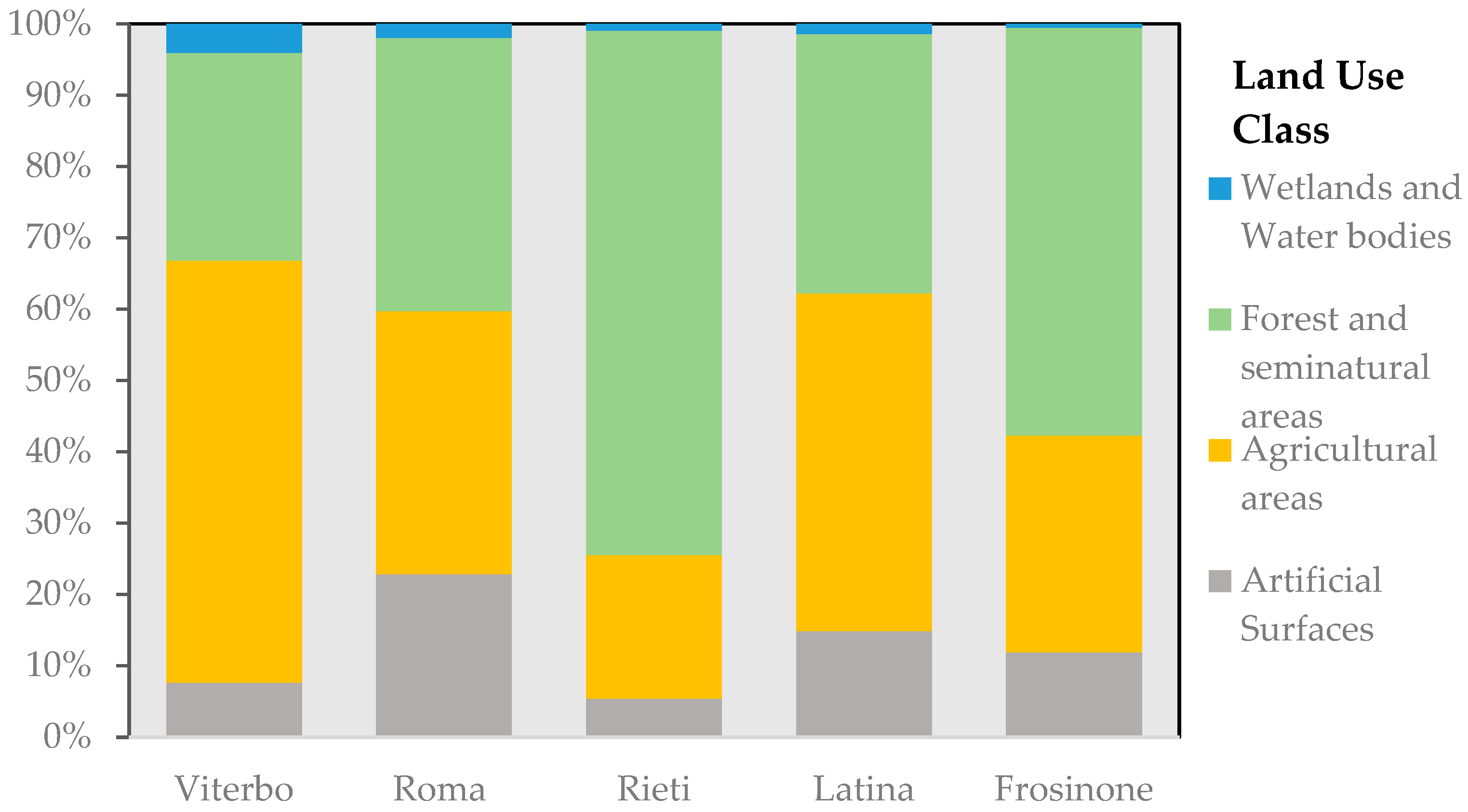
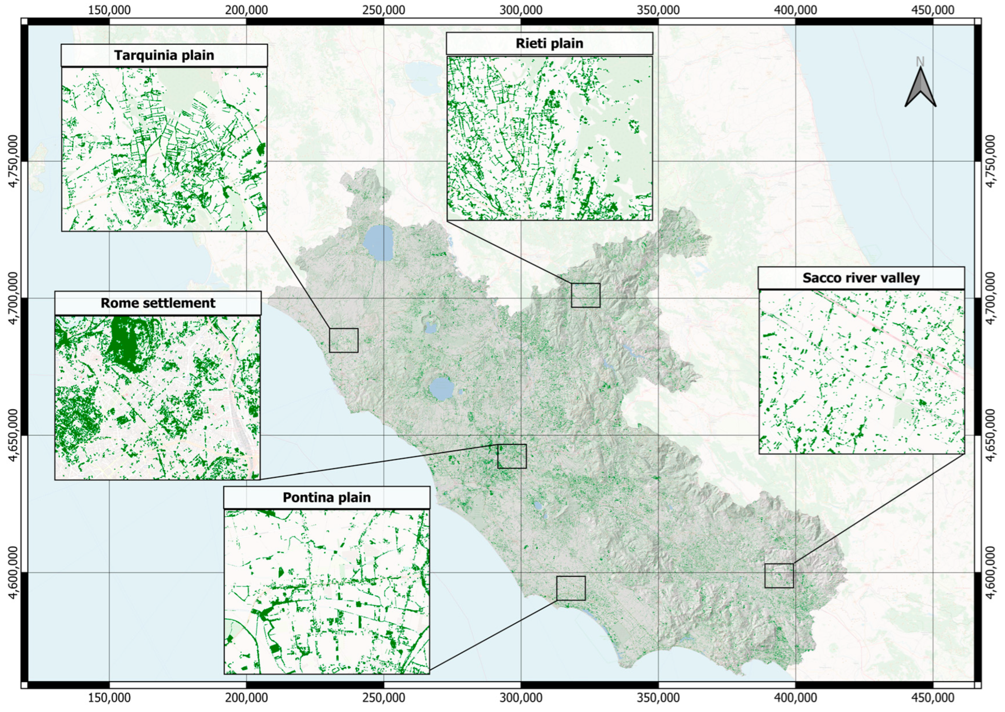
2.1. Study Area

The study area was Lazio, a region in central Italy, located between 11°26′ and 14°01′ E and 40°47′ and 42°50′ N. It covers an area of 17,242 km2 and is divided into five provinces: Viterbo, Rieti, Rome, Frosinone, and Latina. The region is characterized by a Mediterranean climate in the coastal and hilly areas with mild temperatures (9 °C in winter and 24 °C in summer) and low precipitation (700 mm/year), while in the Apennine areas, a continental climate is found, with winter temperatures below 0 °C and abundant precipitation (1200 mm/year) [60,61]. Elevations range from 0 m above sea level in coastal plain areas to areas of the Apennine Mountain range with altitudes exceeding 2000 m above sea level.
The land use classes in the study area are as follows (1st level CORINE Land Cover): artificial surfaces cover 13.7%, 39.1% is represented by utilized agricultural areas, 45.3% is forested areas and seminatural environments, while wetlands and water bodies comprise 1.9% (Figure 1).

2.2. Data

The analyses conducted in this study utilized the AGEA orthophoto from 2017, Sentinel-2 images, the forest type map, the “Small Woody Feature” layer developed by Copernicus [62], and the Land Parcel Identification System (LPIS) [63].

2.2.1. Orthophoto AGEA

The Italian Agency for Agricultural Payments (AGEA) provides a high-resolution spatial raster data (0.20 m) orthophoto captured every 3 years for land use mapping. This is obtained using a multispectral sensor, allowing data capture in the visible (RGB) and infrared bands. This study utilized the 2017 AGEA orthophoto. Downsampling was carried out using QGIS 3.16 software [64] to accelerate the image processing, reducing the spatial resolution from 0.20 m to 2.5 m. The choice of 2.5 m enhanced the cartographic products significantly while retaining the capability to identify small SWFs (i.e., isolated trees).

2.2.2. Sentinel-2 Datasets

Sentinel-2 satellites are equipped with a multispectral sensor offering 13 bands at spatial resolutions between 10 to 60 m and a 5-day temporal resolution. For this study, top of atmosphere reflectance images were downloaded. For the spring season, the April images were chosen to detect summer crops with low soil cover, while the June and July images captured the senescence of winter crops and increased the diversity with tree elements. Due to the study area’s location, multiple Sentinel-2 tiles were analyzed, as illustrated in the Supplementary Materials. The pre-processing of Level-1C images involved atmospheric and terrain corrections using SNAP 8.0.0 software and the Sen2Cor processor, employing a 30-m SRTM digital elevation model [65]. Subsequently, NDVI maps at a 10-m resolution were generated for the spring and summer seasons using mosaic techniques to eliminate clouds and to mask the remaining cloudy areas (Figure 2).

2.2.3. Forest Mask

The forest typology map (hereafter referred to as CF) [66] from the Lazio region was used as the forest mask. This map was produced by refining the IV and V-level Corine Land Cover data from the land use map (hereafter CUS). The refinement process involved the visual interpretation of high-resolution images (ADS40 aerial images with a resolution of 0.5 m) and satellite images from the SPOT5 HRG satellite with a resolution of 10 m to identify forest types characterized by ecological, floristic, and cultivation uniformity. The CF was released in vector format at a scale of 1:25,000 in 2011 and updated in December 2012. The data are provided with an overall geometry accuracy of 81.4%.
The CF was rasterized with a spatial resolution of 2.5 m using QGIS 3.16 software.

2.2.4. Small Woody Features

Small Woody Features (SWF-ESA) is a dataset produced by the Copernicus European Space Agency (ESA) program, available for download from the Land Monitoring Service website. This dataset covers the entirety of Europe and details vegetation such as hedges, shrubs, and trees. It was generated using high-resolution images from various commercial satellites such as Pleiades, WorldView, and Spot, with 5 m and 100 m spatial resolutions. The elements included in the SWF 2015 mapping comprise linear hedges, tree rows, and isolated trees, while artificial elements such as tree plantations and vineyards are excluded.
The data are provided with a thematic accuracy level for the entire European Union exceeding 81.9 for the producer’s accuracy and 79.9 for user’s accuracy. However, the validation only concerns the 100 m raster data, and the authors themselves state that the accuracy metrics obtained do not reflect the quality of the 5 m raster.

2.2.5. LPIS Data

The Land Parcel Identification System (LPIS) is a system based on aerial or satellite photographs recording all agricultural parcels in the Member States. In Italy, it is based on cadastral parcels integrated by photointerpretation for surfaces not included in the database. The LPIS was rasterized with a spatial resolution of 5 m using QGIS 3.16 software to identify orchards and overcome errors of classification.

2.2.6. Reference Data

The accuracy assessment of the classification of NVC and SWF maps was based on the photointerpretation of the AGEA orthophoto. Using the same image for segmentation and classification avoided potential errors arising from the land use variations. Randomly distributed points were photointerpreted across the study area for the training and validation sets using QGIS 3.16 software.

2.3. Image Processing Method

GIS and remote sensing techniques were employed to map the SWFs using QGIS 3.16 and Orfeo Toolbox 7.4.0 software. The main phases of the workflow include:
  • Object-oriented classification of the AGEA orthophoto (RGB) at 2.5 m was used to identify the natural vegetation cover (NVC), which has been proven to be effective for heterogeneous areas [67,68]. For this purpose, we used the segmentation large scale mean shift algorithm implemented in the Orfeo Toolbox 7.4.0 software. The artificial neural network (ANN) algorithm was used for binary classification, distinguishing between NVC and other land use (OLU) [69];
  • Mapping fog SWFs (SWF-UN): The NVC map was stratified into SWF, forest, and other land uses using spectral data, vegetation info, and CF. The classification was refined by setting the NDVI threshold and forest pixel overlap threshold, while LPIS data were used to exclude orchards and minimize errors;
  • Comparison of the produced SWF-UN map with the SWF-ESA and EFA maps by standardizing data and masking forest areas using the LULCC package in R Studio [70].
For details regarding the proposed procedure, refer to the Supplementary Materials.

2.4. Validation

In this study, validation of the NVC map was initially performed, followed by validation of the produced SWF maps. Additionally, the same reference points were utilized to validate the SWF-ESA data and EFA class of LPIS data. Validations were conducted using confusion matrices, and the following statistics were employed: overall accuracy (OA), producer’s accuracy (PA), and user’s accuracy (UA) for the NVC map. Conversely, for the SWF-UN and SWF-ESA maps, producer’s accuracy (PA) and user’s accuracy (UA) metrics were considered. PA represents the percentage of SWF-UN reference points correctly classified as SWF-UN in the map, while UA indicates the percentage of correctly classified SWF-UN class pixels. SWF-UN accuracy assessment was performed for the following areas: the entire Lazio region, each province within the Lazio region, three land use classes, and three altitudinal zones (areas <300 m a.s.l., areas 300–600 m a.s.l., and areas >600 m a.s.l.). All confusion matrices and statistics were computed using the ASBIO package [71] in R 4.1.2.

3. Results

In this section, we present the results of this study, which were divided into two main categories:
  • Accuracy assessment of NVC maps and SWF-UN map: The first part of this section focuses on the accuracy assessment of the NVC map and SWF-UN map. The varying landscape complexity due to factors such as elevation or different production systems can lead to classification errors. Additionally, in Lazio, the different provinces are very diverse in terms of landscape structure, both morphologically and in terms of production systems. To take into account the factors that can affect the quality of classification, validation was performed considering different spatial scales. The validation was conducted including regional and provincial levels as well as different land use macroclasses (settlements, agricultural areas, non-settlements/agricultural areas) and altitudinal zones (areas < 300 m a.s.l., areas 300–600 m a.s.l., and areas > 600 m a.s.l.).
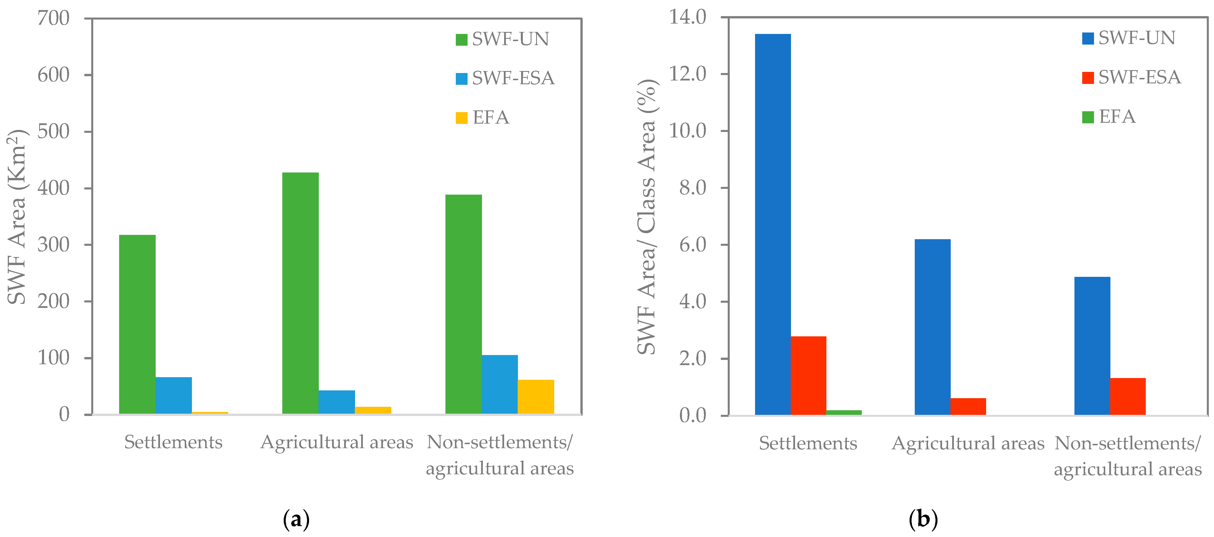
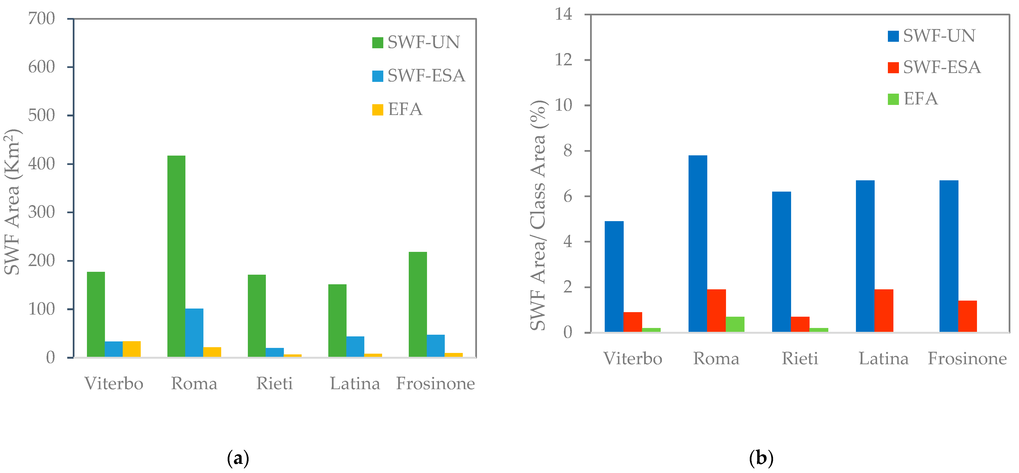
  • Comparison with existing layers: The second part of this section examines the comparison between the SWF-UN map and other existing layers, namely the SWF-ESA and EFA. This comparison aimed to evaluate the consistency and agreement between the SWF-UN map and established datasets, providing insights into the accuracy and reliability of our mapping approach.

3.1. Accuracy Assessment of NVC Map

The result of the accuracy assessment obtained from the classification is shown in Table 1. The analysis revealed that the classification resulted in high OA accuracy values, particularly with the NVC class identified by UA and PA values exceeding 86%. However, the NVC map tended to underestimate the representation of the NVC class in the territory, exhibiting a commission error of 9% and an omission error of 14%.
Subsequent validation of the SWF maps for the macro-areas of analysis enabled the localization and explanation of these confusion errors.

3.2. Accuracy Assessment of SWF Map

Two different maps of the SWF were generated: the first with a spatial resolution of 2.5 m where the orchards were kept, and the second one with a spatial resolution of 5 m and with the orchards masked. Accuracy assessment was carried out on both maps since the tree crops were very widespread in some areas and could affect the classification.

3.2.1. SWF Map at 2.5 m

The accuracy assessment of the SWF-UN map for the Lazio region, as detailed in Table 2, showed a high overall accuracy (OA) value, with commission and omission errors of 27.8% and 9.5%, respectively, indicating an overestimation of SWF areas. Among the different land use categories, the analysis showed the highest OA value for “Non-settlements/Agricultural areas”, while the lowest value was obtained for “Agricultural areas”. Further examination of the user’s accuracy (UA) revealed that the “Agricultural areas” class exhibited a higher commission error while representing areas with the lowest omission error, confirming the difficulty in detecting SWFs in this areas. Similarly, high OA values were observed for provincial validations. Analysis of the UA indicated that the provinces of Viterbo and Latina exhibited more significant commission errors, probably due to the relevant presence of orchards. Regarding elevation, the highest OA was obtained for areas above 600 m a.s.l., although a high commission error and the absence of omission errors were noted. Analysis of the accuracy of individual SWF classes indicated that the UA was lower than the producer’s accuracy (PA), suggesting an overestimation of SWFs.

3.2.2. SWF-UN Map at 5 m

The results of the accuracy analysis of the 5 m resolution SWF mapping are presented in Table 3, covering a total area of 1134 km2 across the regional territory (Figure 3).
The accuracy evaluation of the SWF mapping of the entire Lazio region showed high OA values, comparable to those of the 2.5 m resolution map, with omission and commission errors of 21.5% and 18.1%, respectively. A comparison of the UA and PA between the 2.5 m and 5 m resolution maps revealed that the commission error associated with the 2.5 m map was higher by 6.3%, while the omission error for the 5 m map was higher by 7.6%. Similar results to the validation of the 2.5 m SWF-UN map were observed across different land use categories, with the highest OA value found for “Non-settlements/Agricultural areas”, and the lowest for “Agricultural areas”. Analysis of the UA and comparison with the 2.5 m SWF-UN map showed a decrease in commission error (−11.8%) and an increase in omission error (+12.8%). Among the different land use types, the “Non-settlements/Agricultural areas” class exhibited the highest omission errors at 34%.
Evaluation of the accuracy matrices at the provincial scale for the 5 m SWF-UN map revealed significant improvements for the province of Viterbo, with the commission error decreasing from 39.3% to 19.3%, while the omission error increased from 15.0% to 25.4%. A similar trend was observed for the province of Latina, with a decrease in commission error (−5.1%) and an increase in omission error (+13.9%) confirming the importance of excluding orchards from the evaluation.

3.2.3. SWF-ESA 2015 at 5 m

The validation report of the SWF-ESA 2015 dataset for the Italian area showed a producer’s accuracy (PA) exceeding 80.45%, while the user’s accuracy (UA) was over 72.7%. Based on these metrics, the SWF-ESA layer showed more commission errors than omission errors. However, the validation of the 5 m resolution layer produced significantly different results (Table 4). The validation conducted over the entire Lazio region showed a commission error of 6.7%; however, the omission error was high at 76.1%, indicating an underestimation of linear features. This trend was observable in each validated sub-area; the lowest commission errors were found in the provinces of Rieti and Frosinone (0%), and the elevation band between 300 and 600 m (0%). However, sub-areas with higher UA values were characterized by more significant omission errors, with Rieti at 80.4%, Frosinone at 83.1%, and the elevation band of 400–600 m at 86.5%. In ‘Non-settlements/Agricultural areas’ and regions above 600 m in elevation, a UA of 100% was observed; nevertheless, an accuracy assessment could be conducted with fewer than 10 data points.

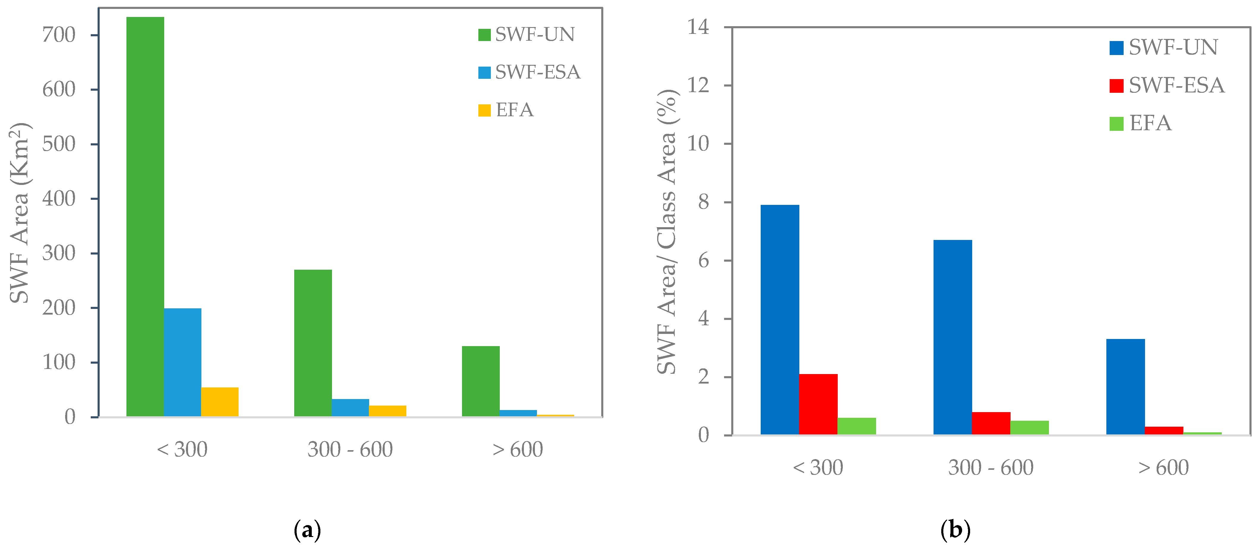
3.3. Comparison of SWF-UN Map with Other SWF Data

From the mapping of SWF-UN, a total area of 1134 km2 was identified. These data were compared with the SWF-ESA map (245 km2) and the EFA (79 km2), revealing significant differences in the identified areas. For a more accurate assessment, SWF data were compared using macro-categories. Figure 4 shows that the “Agricultural areas” class had the highest number of SWFs for the SWF-UN data, while for the SWF-ESA and EFA data, “Non-settlements/Agricultural areas” showed a higher presence of SWFs, being the most represented macroclass in the Lazio region (7972 km2). Additionally, the SWF-UN and SWF-ESA data identified a higher presence of SWFs in the “Settlements” and “Non-settlements/Agricultural areas” classes than the EFA data. The analysis revealed that the percentages of “Agricultural areas” occupied by SWFs were respectively 6.2% for the SWF-UN data, 0.6% for the SWF-ESA data, and less than 0.1% for the EFA data.
The “Settlements” and “Non-settlements/Agricultural areas” classes had a comparable SWF surface area for the SWF-UN data. However, the extent of “Non-settlements/Agricultural areas” was higher than that of “Settlements” (7972 km2 vs. 2369 km2), resulting in a SWF-UN percentage of 4.9% compared to 1.3% for the SWF-ESA data, while the EFA data identified a significantly lower surface area, less than 1%.
Similarly, for the “Settlements” class, a higher detection of SWFs was observed from the newly produced layer compared to the existing layers, indicating a high presence of SWFs in these areas, amounting to 13.4% of the overall surface area of the class.
The second analysis focused on provincial areas (Figure 5). Across all provinces, the SWF-UN map identified more SWFs than the SWF-ESA and EFA maps. Concerning the SWF-UN map, Rome had the largest SWF area among the provinces, while Latina had the smallest. However, when considering the SWF-to-area ratio, Rome had the highest percentage of SWFs (7.8%), whereas Viterbo had the lowest percentage at only 4.9%. It is worth noting that in Viterbo province, while SWF-UN identified numerous SWFs, both the SWF-ESA and EFA data identified an equal number of SWFs, accounting for 0.9 per cent of the provincial area each. In the SWF-ESA data, Rome had the largest SWF area, with Frosinone and Latina having equal SWF areas, followed by Viterbo. Regarding the EFA data, Viterbo had the most SWFs, while Rieti, Latina, and Frosinone had similar SWF areas (0.2% and 0.3%).
From the evaluation of SWFs in the altitude bands (Figure 6), the highest presence of SWFs was identified in the plain class (<300 m), accounting for 7.9% of the plain area (9250 km2). The SWF-ESA and EFA data also confirmed this. Conversely, the area with the lowest level of mapped SWFs was the mountainous region (>600 m above sea level), with respective percentages of 3.3% for the SWF-UN data, 0.3% for the SWF-ESA data, and 0.1% for the EFA data.
Despite significant differences in surface area identification among various data sources, it is essential to examine how SWFs are distributed in “Agricultural areas” at the provincial level, given their crucial ecological function and the variety of land management practices.
The results of the analysis of SWFs in “Agricultural areas” in each province are presented in Figure 7. The SWF-UN map showed that Rome had the largest SWF surface area, while Latina had the least. Conversely, the SWF-ESA data indicate that Rieti had the smallest SWF surface area. Interestingly, the EFA data suggest a larger SWF surface area in the “Agricultural areas” of Viterbo province, which contradicts other datasets and hints at EFA’s limited inclusivity in the “Settlements” and “Non-settlements/Agricultural areas” categories.
In Figure 7b, the percentage of SWFs in “Agricultural areas” for each province is shown. A higher SWF percentage could be observed in Rieti province according to the SWF-UN map (10.2%), whereas in Viterbo province, the percentage dropped to 4.1%. SWF-ESA data showed less variation in SWF percentages, with Frosinone having the highest (2.1%) and Viterbo the lowest (0.8%). EFA data indicated the highest SWF percentage in Viterbo province (1.2%), with other provinces showing comparable values averaging 0.9% (St.Dev = 0.2%).
From the comparison between Figure 5b and Figure 7b, it can be observed that for the SWF-UN map, the province of Rieti had a higher percentage presence of SWFs in agricultural areas than the entire provincial surface (+4.0%). In contrast, for the provinces of Rome and Latina, a lower incidence of SWFs in “Agricultural areas” was highlighted (−2.0%). The SWF-ESA data showed very slight differences for each province; however, for Rieti and Frosinone, a higher incidence of SWFs in “Agricultural areas” was found at +0.6% and +0.7%, respectively, while no differences were observed in Latina. The EFA map showed a higher percentage incidence of SWFs in provincial agricultural areas compared to the total land use.
A transition matrix (Table 5) was utilized to compare the effectiveness of SWF detection in the new layer produced versus the existing layers. The comparison between SWF-UN and SWF-ESA revealed that 996 km2 was missing from the SWF-ESA data, whereas 107 km2 was missing from the SWF-UN data. This result was expected, as it is consistent with the underestimation of SWFs highlighted by the SWF-ESA data (omission error = 76.1%). To assess the reliability of the SWFs omitted from the SWF-UN and SWF-ESA maps, 1684 randomly distributed points in the excluded areas within the study area were evaluated. The analysis showed that 73.7% of the elements classified by the SWF-UN map and omitted from the SWF-ESA data were correctly classified as SWFs, while out of the elements omitted from SWF-UN and mapped by SWF-ESA, only 51.3% were correctly classified.
Comparing the SWF-UN map with the EFA data, significant differences were highlighted, particularly the SWF-UN layer, which identified 1105 km2 more than the EFA data, whereas both layers identified 29 km2. An accuracy assessment was conducted by placing random points (n = 2064) on the SWFs, which was identified solely by one layer. The analysis revealed that surfaces identified solely by the SWF-UN data had an accuracy of 75.9%, while SWFs identified solely by the EFA layer had an accuracy of 50.9%.

4. Discussion

The absence of an inventory and monitoring program for SWFs poses a significant challenge for effective land management, making the widespread localization and quantification of SWFs difficult to achieve. Additionally, photointerpretation and field surveys are costly operations. On the other hand, land use maps are commonly produced at a resolution that is too low to detect SWFs [56].
To address these issues, this study proposed a methodology for SWF mapping over a wide area using satellite and aerial imagery acquired periodically. The obtained map was compared with other existing maps to assess its quality. In the study area, an overall accuracy of the final SWF-UN map of 86.7% was achieved, a result comparable to the overall accuracy reported in other studies [30,35]. However, none of the previous studies utilized a multitemporal analysis to define the NDVI thresholds, and the study areas were commonly smaller (e.g., municipalities or smaller) [51,58]. For the application of the proposed methodology in other study areas, it is necessary to consider the definition of forests, allowing for the generation of a complementary cartographic product to forest surface mapping.
The identification of SWFs in agricultural areas is important as they provide crucial ecosystem functions and services. Across the three evaluated layers, a consistent result could be observed with most SWFs located in agricultural areas. This was an expected outcome as SWFs are closely associated with agricultural management and often define the true territorial identities [72,73]. For instance, it is common to find tree-lined hedges that mark boundaries between parcels or in pastoral areas and field trees that serve as shelter and resting places for livestock [31]. However, there was a significant difference between the SWF layers, with the SWF-UN layer identifying 428 km2 compared to the 14 km2 of the EFA layer and the 42 km2 of the SWF-ESA layer.
The main difficulties encountered concerned the management of high-resolution spatial data for image processing, resulting in increased processing times. In some cases, the LSMS segmentation algorithm failed to perfectly identify the shape of the SWFs, mainly due to the high-resolution RGB image, which did not clearly distinguish herbaceous vegetation from SWFs. This issue was especially prominent in higher-altitude pasture for areas > 600 m a.s.l., where a lower PA value (65.5%) was observed compared to other altitude ranges (areas < 300 m a.s.l PA = 70.9%, areas 300–600 m a.s.l. PA = 77.0%); this result is due to commission errors with green pasture areas. Another critical element is the characterization of segmentation polygons with NDVI data obtained from Sentinel-2, as SWFs often have a size smaller than the minimum pixel unit of 10 m × 10 m; therefore, a pixel may contain more than one land cover/use type, leading to omission or commission errors [30].
From the validation performed per province, areas with the worst classification performance emerged. Despite showing high OA (77.9%) and UA (85.0%) values in Viterbo province, the PA values were lower than 62%. In Latina province, OA (77.1%) and UA (96.7%) values were obtained, while the PA value was the lowest obtained (57.6%). For both validation areas, the low PA value was due to numerous confusion errors with the “Other land use” class, mainly caused by the high presence of orchards (i.e., hazelnut (Corylus avellana L.) for Viterbo and Actinidia (Actinidia Lindl.) for Latina), which exhibit a spectral behavior similar to forest species.
The comparison with other existing SWF maps showed a more remarkable ability of the SWF-UN map to identify the presence of these landscape elements, revealing significant areal differences. These differences may be due to various factors: the scale of application, the technique used, the map production format, and the purpose for which the data is produced. The first difference considered was the scale of application; while the EFA and SWF-UN layers were developed for the Lazio region, the SWF-ESA layer was part of a program at the European scale. The EFA and SWF-UN data were comparable regarding the application scale, but the methodology used were quite different. The EFA layer, produced through photointerpretation, only identified 79 km2 of SWFs in the Lazio region, and a comparison with other data revealed that the accuracy percentage was below 61%. This low accuracy may be due to limitations associated with photointerpretation, where different operators may have used different criteria for identifying the SWFs.
Furthermore, the EFA data were obtained from the LPIS, whose purpose is not to obtain landscape linear elements, but rather to produce a complete land use map of the Lazio region. Another issue concerns the data production mode; as the EFA data are provided in vector format, rasterization is necessary for comparison. The rasterization operation resulted in the loss of SWF surface area as some elements had a size smaller than the minimum pixel unit.
The SWF-ESA data were produced from remote sensing data with a comparable methodology to the SWF-UN data; however, the different criteria used for mapping and the different scales of representation may explain the different mapped surfaces. According to Italian regulation, a forest area is an area covered by trees with a minimum surface of 2000 m2 and a width exceeding 20 m [74].
The SWF-ESA layer was rasterized at 5 m resolution from a vector layer where SWF structures were delineated based on the following specifications: a maximum width of 30 m and a minimum length of 50 m for linear features, and a minimum and maximum area of 200 and 5000 m2, respectively, for patches and additional features. This implies that some surfaces can be identified and classified as forest or not depending on the scale and the criteria used, thus influencing the mapping of SFWs.
The proposed classification approach could be applied to any aerial image and is valid for large-scale SWF mapping. High-resolution aerial images are the reliable data needed to derive the geometric thresholds. The Sentinel-2 mission is a valuable tool for monitoring the physiological parameters of vegetation.
For Italy, the agricultural monitoring program of AGEA represents an important opportunity for mapping and monitoring SWFs at the national scale and for integrating the forest inventory. This study could be considered as a test methodology for application at the national level and will help integrate information on SWF resources into land-cover databases, thereby filling a critical spatial SWF information gap in landscape management.
In fact, although the SWF-ESA data were obtained from very-high resolution images, the geometric specification used for the identification of SWFs may exclude some elements that can be important for analysis conducted at a more local scale. As reported in the Copernicus Land Monitoring Service 2018, this is especially true in complex landscapes such as in Mediterranean areas or in Scandinavian landscapes, where low density open forest is frequent, or, as reported in Danijel et al. (2024) [75], in areas with high landscape heterogeneity (Slovenia and the Goričko region), where the Small Woody Features (SWFs) vector database obtained from the Copernicus web platform has limited value [62]. Weaknesses in the SWF database from the Slovenian landscape perspective has encouraged the National Institute for Nature Conservation (IRSNC) to study the detection of small woody landscape features. Therefore, with the proposed method, countrywide investigations might become more feasible for other countries encountering the necessity of detailed local information.
Some authors have utilized LiDAR or radar-derived canopy height models to create maps showing the distribution of different types of vegetation (such as hedgerows, shrubs, isolated trees, groves, etc.) [58,76]. For Italy, LiDAR data are not always available for large areas such as the Lazio region. Therefore, the aim of this work was to verify the possibility of identifying SWFs using only easily accessible and low-cost data. Of course, a challenging task for future developments is the height dimension of linear SWFs. This parameter can also provide valuable information about the services offered by these linear features in the landscape and their potential role in agriculture sustainability. Recognizing and harnessing this potential could have significant implications for the field. SWFs can be essential in situations where both conventional and organic agricultural farming coexist. In the European Green Deal context, organic farming is seen as a management system that contributes to the EU’s overall goal of achieving carbon neutrality. This is further outlined in the Farm to Fork Strategy, which introduces an action plan for organic farming that aims to convert at least 25% of the EU’s agricultural land to organic farming by 2030 [77]. Consequently, the expansion of organic farming may lead to increased land use conflicts near conventional farms. In this scenario, vertical SWFs can act as a barrier, helping to prevent chemical drifting.
However, separating SWF types by multispectral and optical images to monitor and map their capabilities in preventing drifting can be challenging. A significant amount of ground truth data are needed to enhance the identification of the dimensional characteristics of SWFs. Acquiring a large number of ground truths is a time-consuming process and is one of the main challenges in remote sensing applications. Nonetheless, crowdsensing platforms offer a potential solution by involving voluntary contributors in gathering ground truth data. One example is the “Eye-Land” project, which developed an app to collect ground truth data including 3D and point clouds for remote sensing applications [78].
The method described in this paper is simple and cost-effective for mapping SWFs on a wide scale; it could help other countries to create their own datasets of SWFs as input for environmental policymaking, forest policy, or similar elements to define a strategy for the challenges of climate change and the environment. The proposed methodology represents the first step of a broader work: in this initial step, a methodology was sought to accurately map, at a regional scale, the SWFs (small landscape features) that play an important role in landscape characterization. The next step will involve using these elements to describe the landscape mosaic and linking these minor elements with the functional aspects of the landscape to better understand the interactions between land management, landscape structure, and ecosystem functioning.

5. Conclusions

This study used a semi-automated approach to SWF mapping for the Lazio region (17,242 km2) by utilizing a high-resolution RGB image and multispectral image. The novel SWF-UN map identified 6.6% of the region as covered with SWFs. The proposed methodology investigated the distribution of SWFs in various sub-areas: provinces, altitude bands, and land use macroclasses.
The description of the applied method and utilized materials enables the repeatability of the process and its extension to other regional or national study areas. In the present study, reliable results were achieved with a high overall accuracy (OA) of 0.86 and user’s accuracy (UA) of 0.82, along with a good producer’s accuracy (PA) of 0.78. Furthermore, the new SWF-UN map provided a more accurate representation of SWF distribution in the territory compared to existing layers, allowing for the identification of 1134 km2 of SWFs with an accuracy exceeding 73.7%. Despite the availability of informational layers at the European scale, the results obtained demonstrate the need for further refinement of the procedures used when conducting detailed studies at the local scale.
With the new SWF-UN layer, new analyses can be defined to deepen and evaluate the understanding of agricultural territory. This study demonstrates that the use of high-resolution spatial images, in synergy with multispectral images, represents beneficial and essential elements for SWF monitoring at the regional scale and can serve as a starting point for further research.

Supplementary Materials

The following supporting information can be downloaded at: https://www.mdpi.com/article/10.3390/land13081128/s1, Detailed description of the proposed methodology; Figure S1: The study area is indicated in red. The extent of the respective S2 tiles (in black) is also indicated, along with ESA’s scene naming convention. Table S1: List of Sentinel-2 images used in this study. Figure S2: Examples of SWF identification in areas with different land cover for the three datasets. Forest areas are shown in red, and SWFs are shown in green.

Author Contributions

Conceptualization, A.P., F.R., E.M., and M.N.R.; Methodology, A.P., M.N.R., and F.R.; Software, C.M.R. and A.P.; Validation, A.P., C.M.R., and E.C.; Investigation, A.P., E.C., and L.G.; Data curation, A.P.; Writing—original draft preparation, A.P., L.G., and E.M.; Writing—review and editing, A.P., E.C., C.M.R., E.M., M.N.R., and F.R.; Supervision, F.R. and M.N.R.; Funding acquisition, M.N.R. All authors have read and agreed to the published version of the manuscript.

Funding

This research was funded by Agenzia Regionale per lo Sviluppo e l’Innovazione dell’Agricoltura del Lazio: rep. n.119—21/12/2020.

Data Availability Statement

Data are available on request. These data were derived from the following resources available in the public domain: https://dataspace.copernicus.eu/, https://openiacs.eu/dataset/open-iacs_iacs_it_2020_lpis, https://land.copernicus.eu/ accessed on 5 January 2022. The original data produced in this article are not readily available because the data are part of an ongoing study.

Acknowledgments

The research was carried out within the framework of the Ministry of University and Research (MUR) initiative “Departments of Excellence” (Law 232/2016) DAFNE Project 2023-2027 “Digital, Intelligent, Green and Sustainable (D.I.Ver.So)”.

Conflicts of Interest

The authors declare no conflicts of interest.

References

  1. Gámez-Virués:, S.; Perović, D.J.; Gossner, M.M.; Börschig, C.; Blüthgen, N.; de Jong, H.; Simons, N.K.; Klein, A.-M.; Krauss, J.; Maier, G.; et al. Landscape Simplification Filters Species Traits and Drives Biotic Homogenization. Nat. Commun. 2015, 6, 8568. [Google Scholar] [CrossRef]
  2. Oliver, T.H.; Morecroft, M.D. Interactions between Climate Change and Land Use Change on Biodiversity: Attribution Problems, Risks, and Opportunities. WIREs Clim. Change 2014, 5, 317–335. [Google Scholar] [CrossRef]
  3. Dash, P.; Punia, M. Governance and Disaster: Analysis of Land Use Policy with Reference to Uttarakhand Flood 2013, India. Int. J. Disaster Risk Reduct. 2019, 36, 101090. [Google Scholar] [CrossRef]
  4. García-Ruiz, J.M. The Effects of Land Uses on Soil Erosion in Spain: A Review. CATENA 2010, 81, 1–11. [Google Scholar] [CrossRef]
  5. Roossinck, M.J.; García-Arenal, F. Ecosystem Simplification, Biodiversity Loss and Plant Virus Emergence. Curr. Opin. Virol. 2015, 10, 56–62. [Google Scholar] [CrossRef] [PubMed]
  6. Zucca, C.; Canu, A.; Previtali, F. Soil Degradation by Land Use Change in an Agropastoral Area in Sardinia (Italy). CATENA 2010, 83, 46–54. [Google Scholar] [CrossRef]
  7. Bellefontaine, R.; Petit, S.; Pain-Orcet, M.; Deleporte, P.; Bertault, J.-G. Trees Outside Forests—Towards a Better Awareness. In Proceedings of the FAO Conservation Guide 35; FAO: Rome, Italy, 2002. [Google Scholar]
  8. FAO. Trees Outside Forests: Towards Rural and Urban Integrated Resources Management; FAO: Rome, Italy, 2001. [Google Scholar]
  9. Collier, M.J. Are Field Boundary Hedgerows the Earliest Example of a Nature-Based Solution? Environ. Sci. Policy 2021, 120, 73–80. [Google Scholar] [CrossRef]
  10. Frank, S.; Fürst, C.; Witt, A.; Koschke, L.; Makeschin, F. Making Use of the Ecosystem Services Concept in Regional Planning—Trade-Offs from Reducing Water Erosion. Landsc. Ecol. 2014, 29, 1377–1391. [Google Scholar] [CrossRef]
  11. Chen, J.; Xiao, H.; Li, Z.; Liu, C.; Ning, K.; Tang, C. How Effective Are Soil and Water Conservation Measures (SWCMs) in Reducing Soil and Water Losses in the Red Soil Hilly Region of China? A Meta-Analysis of Field Plot Data. Sci. Total Environ. 2020, 735, 139517. [Google Scholar] [CrossRef] [PubMed]
  12. Skole, D.L.; Mbow, C.; Mugabowindekwe, M.; Brandt, M.S.; Samek, J.H. Trees Outside of Forests as Natural Climate Solutions. Nat. Clim. Change 2021, 11, 1013–1016. [Google Scholar] [CrossRef]
  13. Golicz, K.; Ghazaryan, G.; Niether, W.; Wartenberg, A.C.; Breuer, L.; Gattinger, A.; Jacobs, S.R.; Kleinebecker, T.; Weckenbrock, P.; Große-Stoltenberg, A. The Role of Small Woody Landscape Features and Agroforestry Systems for National Carbon Budgeting in Germany. Land 2021, 10, 1028. [Google Scholar] [CrossRef]
  14. Reyes, F.; Gosme, M.; Wolz, K.J.; Lecomte, I.; Dupraz, C. Alley Cropping Mitigates the Impacts of Climate Change on a Wheat Crop in a Mediterranean Environment: A Biophysical Model-Based Assessment. Agriculture 2021, 11, 356. [Google Scholar] [CrossRef]
  15. Ritchie, H.; Samborska, V.; Roser, M. Urbanization; Our World Data: Oxford, UK, 2024. [Google Scholar]
  16. Holt-Gimenez, E. Can We Feed the World Without Destroying It? John Wiley & Sons: Hoboken, NJ, USA, 2019; ISBN 978-1-5095-2204-0. [Google Scholar]
  17. Sutter, L.; Albrecht, M.; Jeanneret, P. Landscape Greening and Local Creation of Wildflower Strips and Hedgerows Promote Multiple Ecosystem Services. J. Appl. Ecol. 2018, 55, 612–620. [Google Scholar] [CrossRef]
  18. Zomer, R.J.; Neufeldt, H.; Xu, J.; Ahrends, A.; Bossio, D.; Trabucco, A.; van Noordwijk, M.; Wang, M. Global Tree Cover and Biomass Carbon on Agricultural Land: The Contribution of Agroforestry to Global and National Carbon Budgets. Sci. Rep. 2016, 6, 29987. [Google Scholar] [CrossRef] [PubMed]
  19. Baudry, J.; Bunce, R.G.H.; Burel, F. Hedgerows: An International Perspective on Their Origin, Function and Management. J. Environ. Manag. 2000, 60, 7–22. [Google Scholar] [CrossRef]
  20. Burel, F.; Baudry, J.; Butet, A.; Clergeau, P.; Delettre, Y.; Le Coeur, D.; Dubs, F.; Morvan, N.; Paillat, G.; Petit, S.; et al. Comparative Biodiversity along a Gradient of Agricultural Landscapes. Acta Oecologica 1998, 19, 47–60. [Google Scholar] [CrossRef]
  21. Liccari, F.; Boscutti, F.; Bacaro, G.; Sigura, M. Connectivity, Landscape Structure, and Plant Diversity across Agricultural Landscapes: Novel Insight into Effective Ecological Network Planning. J. Environ. Manag. 2022, 317, 115358. [Google Scholar] [CrossRef] [PubMed]
  22. Manning, A.D.; Fischer, J.; Lindenmayer, D.B. Scattered Trees Are Keystone Structures—Implications for Conservation. Biol. Conserv. 2006, 132, 311–321. [Google Scholar] [CrossRef]
  23. Saunders, D.A.; Hobbs, R.J.; Margules, C.R. Biological Consequences of Ecosystem Fragmentation: A Review. Conserv. Biol. 1991, 5, 18–32. [Google Scholar] [CrossRef]
  24. Garratt, M.P.D.; Senapathi, D.; Coston, D.J.; Mortimer, S.R.; Potts, S.G. The Benefits of Hedgerows for Pollinators and Natural Enemies Depends on Hedge Quality and Landscape Context. Agric. Ecosyst. Environ. 2017, 247, 363–370. [Google Scholar] [CrossRef]
  25. Rusch, A.; Chaplin-Kramer, R.; Gardiner, M.M.; Hawro, V.; Holland, J.; Landis, D.; Thies, C.; Tscharntke, T.; Weisser, W.W.; Winqvist, C.; et al. Agricultural Landscape Simplification Reduces Natural Pest Control: A Quantitative Synthesis. Agric. Ecosyst. Environ. 2016, 221, 198–204. [Google Scholar] [CrossRef]
  26. Holden, J.; Grayson, R.P.; Berdeni, D.; Bird, S.; Chapman, P.J.; Edmondson, J.L.; Firbank, L.G.; Helgason, T.; Hodson, M.E.; Hunt, S.F.P.; et al. The Role of Hedgerows in Soil Functioning within Agricultural Landscapes. Agric. Ecosyst. Environ. 2019, 273, 1–12. [Google Scholar] [CrossRef]
  27. Ghazavi, G.; Thomas, Z.; Hamon, Y.; Marie, J.C.; Corson, M.; Merot, P. Hedgerow Impacts on Soil-Water Transfer Due to Rainfall Interception and Root-Water Uptake. Hydrol. Process. 2008, 22, 4723–4735. [Google Scholar] [CrossRef]
  28. Merot, P. The Influence of Hedgerow Systems on the Hydrology of Agricultural Catchments in a Temperate Climate. Agronomie 1999, 19, 655–669. [Google Scholar] [CrossRef]
  29. Thomas, Z.; Abbott, B.W. Hedgerows Reduce Nitrate Flux at Hillslope and Catchment Scales via Root Uptake and Secondary Effects. J. Contam. Hydrol. 2018, 215, 51–61. [Google Scholar] [CrossRef] [PubMed]
  30. Schnell, S.; Kleinn, C.; Ståhl, G. Monitoring Trees Outside Forests: A Review. Environ. Monit. Assess. 2015, 187, 600. [Google Scholar] [CrossRef] [PubMed]
  31. De Foresta, H.; Somarriba, E.; Temu, A.; Boulanger, D.; Feuilly, H.; Gauthier, M. Towards The Assessment of Trees outside Forests. A Thematic Report Prepared in the Framework of The Global Forest Resources Assessment; FAO: Rome, Italy, 2013. [Google Scholar]
  32. Jose, S. Agroforestry for Ecosystem Services and Environmental Benefits: An Overview. Agrofor. Syst. 2009, 76, 1–10. [Google Scholar] [CrossRef]
  33. Vannucci, A.; Andreoli, M.; Rovai, M. Land Use Change and Disappearance of Hedgerows in a Tuscan Rural Landscape: A Discussion on Policy Tools to Revert This Trend. Sustainability 2022, 14, 13341. [Google Scholar] [CrossRef]
  34. Gulinck, H.; Marcheggiani, E.; Verhoeve, A.; Bomans, K.; Dewaelheyns, V.; Lerouge, F.; Galli, A. The Fourth Regime of Open Space. Sustainability 2018, 10, 2143. [Google Scholar] [CrossRef]
  35. Malkoç, E.; Rüetschi, M.; Ginzler, C.; Waser, L.T. Countrywide Mapping of Trees Outside Forests Based on Remote Sensing Data in Switzerland. Int. J. Appl. Earth Obs. Geoinf. 2021, 100, 102336. [Google Scholar] [CrossRef]
  36. Mosquera-Losada, M.R.; Santiago-Freijanes, J.J.; Rois-Díaz, M.; Moreno, G.; den Herder, M.; Aldrey-Vázquez, J.A.; Ferreiro-Domínguez, N.; Pantera, A.; Pisanelli, A.; Rigueiro-Rodríguez, A. Agroforestry in Europe: A Land Management Policy Tool to Combat Climate Change. Land Use Policy 2018, 78, 603–613. [Google Scholar] [CrossRef]
  37. Rigueiro-Rodríguez, A.; Fernández-Núñez, E.; González-Hernández, P.; McAdam, J.H.; Mosquera-Losada, M.R. Agroforestry Systems in Europe: Productive, Ecological and Social Perspectives. In Agroforestry in Europe: Current Status and Future Prospects; Rigueiro-Rodróguez, A., McAdam, J., Mosquera-Losada, M.R., Eds.; Springer: Dordrecht, The Netherlands, 2009; pp. 43–65. ISBN 978-1-4020-8272-6. [Google Scholar]
  38. Álvarez, F.A.; Mediavilla, G.G.; Estébanez, N.L. Environmental, Demographic and Policy Drivers of Change in Mediterranean Hedgerow Landscape (Central Spain). Land Use Policy 2021, 103, 105342. [Google Scholar] [CrossRef]
  39. Santiago-Freijanes, J.J.; Rigueiro-Rodríguez, A.; Aldrey, J.A.; Moreno, G.; den Herder, M.; Burgess, P.; Mosquera-Losada, M.R. Understanding Agroforestry Practices in Europe through Landscape Features Policy Promotion. Agrofor. Syst. 2018, 92, 1105–1115. [Google Scholar] [CrossRef]
  40. García de León, D.; Rey Benayas, J.M.; Andivia, E. Contributions of Hedgerows to People: A Global Meta-Analysis. Front. Conserv. Sci. 2021, 2, 789612. [Google Scholar] [CrossRef]
  41. Thomas, N.; Baltezar, P.; Lagomasino, D.; Stovall, A.; Iqbal, Z.; Fatoyinbo, L. Trees Outside Forests Are an Underestimated Resource in a Country with Low Forest Cover. Sci. Rep. 2021, 11, 7919. [Google Scholar] [CrossRef] [PubMed]
  42. Santoro, A.; Piras, F.; Fiore, B.; Frassinelli, N.; Bazzurro, A.; Agnoletti, M. The Role of Trees Outside Forests in the Cultural Landscape of the Colline Del Prosecco UNESCO Site. Forests 2022, 13, 514. [Google Scholar] [CrossRef]
  43. Alvarez, F.A.; Gomez-Mediavilla, G.; López-Estébanez, N.; Holgado, P.M. Classification of Mediterranean Hedgerows: A Methodological Approximation. MethodsX 2021, 8, 101355. [Google Scholar] [CrossRef] [PubMed]
  44. Fehrmann, L.; Seidel, D.; Krause, B.; Kleinn, C. Sampling for Landscape Elements—A Case Study from Lower Saxony, Germany. Environ. Monit. Assess 2014, 186, 1421–1430. [Google Scholar] [CrossRef]
  45. León, M.C.; Harvey, C.A. Live Fences and Landscape Connectivity in a Neotropical Agricultural Landscape. Agrofor. Syst. 2006, 68, 15–26. [Google Scholar] [CrossRef]
  46. Perry, C.H.; Woodall, C.W.; Liknes, G.C.; Schoeneberger, M.M. Filling the Gap: Improving Estimates of Working Tree Resources in Agricultural Landscapes. Agrofor. Syst. 2009, 75, 91–101. [Google Scholar] [CrossRef]
  47. Zomer, R.J.; Trabucco, A.; Coe, R.; Place, F.; Van Noordwijk, M.; Xu, J.C. Trees on Farms: An Update and Reanalysis of Agroforestry’s Global Extent and Socio-Ecological Characteristics; World Agroforestry Centre (ICRAF): Nairobi, Kenya, 2014. [Google Scholar]
  48. Foschi, P.; Smith, D. Detecting Subpixel Woody Vegetation in Digital Imagery Using Two Artificial Intelligence Approaches. Photogramm. Eng. Remote Sens. 1997, 63, 493–500. [Google Scholar]
  49. Thornton, M.W.; Atkinson, P.M.; Holland, D.A. A Linearised Pixel-Swapping Method for Mapping Rural Linear Land Cover Features from Fine Spatial Resolution Remotely Sensed Imagery. Comput. Geosci. 2007, 33, 1261–1272. [Google Scholar] [CrossRef]
  50. Thornton, M.W.; Atkinson, P.M.; Holland, D.A. Sub-pixel Mapping of Rural Land Cover Objects from Fine Spatial Resolution Satellite Sensor Imagery Using Super-resolution Pixel-swapping. Int. J. Remote Sens. 2006, 27, 473–491. [Google Scholar] [CrossRef]
  51. Sarti, M.; Ciolfi, M.; Lauteri, M.; Paris, P.; Chiocchini, F. Trees Outside Forest in Italian Agroforestry Landscapes: Detection and Mapping Using Sentinel-2 Imagery. Eur. J. Remote Sens. 2021, 54, 609–623. [Google Scholar] [CrossRef]
  52. Brandt, J.; Stolle, F. A Global Method to Identify Trees Outside of Closed-Canopy Forests with Medium-Resolution Satellite Imagery. Int. J. Remote Sens. 2021, 42, 1713–1737. [Google Scholar] [CrossRef]
  53. Ottosen, T.-B.; Petch, G.; Hanson, M.; Skjøth, C.A. Tree Cover Mapping Based on Sentinel-2 Images Demonstrate High Thematic Accuracy in Europe. Int. J. Appl. Earth Obs. Geoinf. 2020, 84, 101947. [Google Scholar] [CrossRef]
  54. Boggs, G.S. Assessment of SPOT 5 and QuickBird Remotely Sensed Imagery for Mapping Tree Cover in Savannas. Int. J. Appl. Earth Obs. Geoinf. 2010, 12, 217–224. [Google Scholar] [CrossRef]
  55. Liknes, G.C.; Perry, C.H.; Meneguzzo, D.M. Assessing Tree Cover in Agricultural Landscapes Using High-Resolution Aerial Imagery. J. Terr. Obs. 2010, 2, 38–55. [Google Scholar]
  56. Meneguzzo, D.M.; Liknes, G.C.; Nelson, M.D. Mapping Trees Outside Forests Using High-Resolution Aerial Imagery: A Comparison of Pixel- and Object-Based Classification Approaches. Environ. Monit. Assess 2013, 185, 6261–6275. [Google Scholar] [CrossRef]
  57. Puissant, A.; Rougier, S.; Stumpf, A. Object-Oriented Mapping of Urban Trees Using Random Forest Classifiers. Int. J. Appl. Earth Obs. Geoinf. 2014, 26, 235–245. [Google Scholar] [CrossRef]
  58. Bolyn, C.; Lejeune, P.; Michez, A.; Latte, N. Automated Classification of Trees Outside Forest for Supporting Operational Management in Rural Landscapes. Remote Sens. 2019, 11, 1146. [Google Scholar] [CrossRef]
  59. Luscombe, D.J.; Gatis, N.; Anderson, K.; Carless, D.; Brazier, R.E. Rapid, Repeatable Landscape-Scale Mapping of Tree, Hedgerow, and Woodland Habitats (THaW), Using Airborne LiDAR and Spaceborne SAR Data. Ecol. Evol. 2023, 13, e10103. [Google Scholar] [CrossRef]
  60. Moccia, B.; Mineo, C.; Ridolfi, E.; Russo, F.; Napolitano, F. Probability Distributions of Daily Rainfall Extremes in Lazio and Sicily, Italy, and Design Rainfall Inferences. J. Hydrol. Reg. Stud. 2021, 33, 100771. [Google Scholar] [CrossRef]
  61. Salvati, L.; Perini, L.; Sabbi, A.; Bajocco, S. Climate Aridity and Land Use Changes: A Regional-Scale Analysis: Climate Aridity and Land Use Changes. Geogr. Res. 2012, 50, 193–203. [Google Scholar] [CrossRef]
  62. Fraucqueur, L.; Morin, N.; Masse, A.; Remy, P.-Y.; Hugé, J.; Kenner, C.; Dazin, F.; Desclée, B.; Sannier, C. A New Copernicus High Resolution Layer at Pan-European Scale: Small Woody Features. In Proceedings of the Remote Sensing for Agriculture, Ecosystems, and Hydrology XXI, Strasbourg, France, 21 October 2019; Neale, C.M., Maltese, A., Eds.; SPIE: Strasbourg, France, 2019; p. 37. [Google Scholar]
  63. European Court of Auditors. The Land Parcel Identification System: A Useful Tool to Determine the Eligibility of Agricultural Land—But Its Management Could Be Further Improved. Special Report No 25, 2016; Publications Office of the European Union: Luxembourg, Luxembourg, 2016; ISBN 978-92-872-5967-7.
  64. QGIS Development Team. QGIS Geographic Information System 2024; QGIS Development Team: Solothurn, Switzerland, 2024. [Google Scholar]
  65. Farr, T.G.; Rosen, P.A.; Caro, E.; Crippen, R.; Duren, R.; Hensley, S.; Kobrick, M.; Paller, M.; Rodriguez, E.; Roth, L.; et al. The Shuttle Radar Topography Mission. Rev. Geophys. 2007, 45, 2005RG000183. [Google Scholar] [CrossRef]
  66. Chirici, G.; Fattori, C.; Cutolo, N.; Tufano, M.; Corona, P.; Barbati, A.; Blasi, C.; Copiz, R.; Rossi, L.; Biscontini, D.; et al. Map of the Natural and Semi-Natural Environments and Forest Types Map for the Latium Region (Italy). For. -Riv. Selvic. Ecol. For. 2014, 11, 65–71. [Google Scholar] [CrossRef]
  67. Benz, U.C.; Hofmann, P.; Willhauck, G.; Lingenfelder, I.; Heynen, M. Multi-Resolution, Object-Oriented Fuzzy Analysis of Remote Sensing Data for GIS-Ready Information. ISPRS J. Photogramm. Remote Sens. 2004, 58, 239–258. [Google Scholar] [CrossRef]
  68. Burnett, C.; Blaschke, T. A Multi-Scale Segmentation/Object Relationship Modelling Methodology for Landscape Analysis. Ecol. Model. 2003, 168, 233–249. [Google Scholar] [CrossRef]
  69. Pádua, L.; Adao, T.; Hruska, J.; Guimaraes, N.; Marques, P.; Peres, E.; Sousa, J.J. Vineyard Classification Using Machine Learning Techniques Applied to RGB-UAV Imagery. In Proceedings of the IGARSS 2020–2020 IEEE International Geoscience and Remote Sensing Symposium, Waikoloa, HI, USA, 26 September 2020; IEEE: Waikoloa, HI, USA, 2020; pp. 6309–6312. [Google Scholar]
  70. Moulds, S.; Buytaert, W.; Mijic, A. An Open and Extensible Framework for Spatially Explicit Land Use Change Modelling: The Lulcc R Package. Geosci. Model Dev. 2015, 8, 3215–3229. [Google Scholar] [CrossRef]
  71. Aho, K. Asbio: A Collection of Statistical Tools for Biologists; CRC Press: Boca Raton, FL, USA, 2024. [Google Scholar]
  72. Centeri, C.; Renes, H.; Roth, M.; Kruse, A.; Eiter, S.; Kapfer, J.; Santoro, A.; Agnoletti, M.; Emanueli, F.; Sigura, M.; et al. Wooded Grasslands as Part of the European Agricultural Heritage. In Biocultural Diversity in Europe; Agnoletti, M., Emanueli, F., Eds.; Springer International Publishing: Cham, Switzerland, 2016; pp. 75–103. ISBN 978-3-319-26315-1. [Google Scholar]
  73. Oreszczyn, S.; Lane, A. The Meaning of Hedgerows in the English Landscape: Different Stakeholder Perspectives and the Implications for Future Hedge Management. J. Environ. Manag. 2000, 60, 101–118. [Google Scholar] [CrossRef]
  74. TUFF Italian Government. Decreto Legislativo 03/04/2018 n. 34—Testo unico in Materia di Foreste e Filiere Forestali (TUFF); TUFF Italian Government: Rome, Italy, 2018.
  75. Danijel, I.; Nataša, P.; Jaša, G.V.; Daša, D.; Mitja, K.; Sonja, Š.; Igor, Ž.; Jure, Č.; Petra, R.N.; Štefan, K.; et al. A Decision Support System for Effective Implementation of Agro-Environmental Measures Targeted at Small Woody Landscape Features: The Case Study of Slovenia. Landsc. Urban Plan. 2024, 247, 105064. [Google Scholar] [CrossRef]
  76. Ducrot, D.; Masse, A.; Ncibi, A. Hedgerow Detection in HRS and VHRS Images from Different Source (Optical, Radar). In Proceedings of the 2012 IEEE International Geoscience and Remote Sensing Symposium, Munich, Germany, 22–27 July 2012; pp. 6348–6351. [Google Scholar]
  77. European Commission. Communication from the Commission to the European Parliament, the Council, the European Economic and Social Committee and the Committee of the Regions a Farm to Fork Strategy for a Fair, Healthy and Environmentally-Friendly Food System; European Commission: Brussels, Belgium, 2020. [Google Scholar]
  78. Ministry of University and Research. Project PRIN 2020—Sector ERC LS9—Call 2020 Prot. 2020 EMLWTN—Eye-Land: A Crowd-Sensing Geospatial Database for the Monitoring of Rural Areas; Ministry of University and Research: Rome, Italy, 2020.
Figure 1. Land cover stacked bar chart of the Lazio provinces (Corine Land Cover 1° Level/Province area ratio) divided into four land use macroclasses. Artificial surfaces are classified in grey, agricultural areas are in orange, forest and seminatural areas are in green, and wetlands and water bodies are in blue.
Land 13 01128 g001
Figure 2. NDVI from Sentinel-2 images for the study area and for two seasons. (a) Spring NDVI, (b) Summer NDVI.
Land 13 01128 g002
Figure 3. SWF-UN map of the Lazio region (shown in green).
Land 13 01128 g003
Figure 4. Bar plot (a), areas of SWFs for the three land use classes for the evaluated SWF maps (SWF-UN, SWF-ESA, and EFA). (b) Percentage ratio between the area of SWFs and the area of the analyzed macroclasses.
Land 13 01128 g004
Figure 5. In bar plot (a), the SWF surfaces in the provinces of the Lazio region for the evaluated SWFs maps (SWF-UN, SWF-ESA, and EFA). (b) Percentage ratio between the SWF area and the area of the provinces.
Land 13 01128 g005
Figure 6. Bar plot (a), SWF surfaces in the three elevation classes for the evaluated SWF maps (SWF-UN, SWF-ESA, and EFA). (b) Percentage ratio between the area of SWF and the area of the analyzed macroclasses.
Land 13 01128 g006
Figure 7. Bar plot (a), SWF surfaces in the agricultural areas of each province. (b) Percentage ratio between the area of SWF and the total area.
Land 13 01128 g007
Table 1. Confusion matrix and accuracy measures for the identification of NVC.
Classified Data
Reference
data
NVCOLUTotalPA (%)
NVC206721022770.91
OLU337238627230.88
Total240425965000-
UA (%)0.860.92--
OA (%) = 89.0.
Table 2. Accuracy measures of the SWF-UN map at 2.5 m for the different macro study areas.
Validation Based on Number of Test PointsOA (%)UA (%)PA (%)
Lazio Region 343086.772.290.5
Land Use ClassSettlements 19182.785.288.9
Agricultural areas147473.770.491.3
Non-settlements/Agricultural areas176598.075.983.0
ProvincesViterbo73577.960.785.0
Roma108587.679.189.0
Rieti62593.177.990.7
Latina42477.157.696.7
Frosinone56196.692.097.2
Elevation
(m a.s.l.)
<300180580.770.989.1
300–600117792.177.094.2
>60044896.665.5100
Table 3. Accuracy measures of the SWF-UN map at 5 m for the different macro study areas.
Validation Based on Number of Test PointsOA (%)UA (%)PA (%)
Lazio Region 343086.781.978.5
Land Use ClassSettlements19180.185.283.8
Agricultural areas147477.581.878.5
Non-settlements/Agricultural areas176595.074.566.0
ProvincesViterbo73584.480.774.6
Roma108585.882.379.2
Rieti62591.883.779.4
Latina42482.672.782.8
Frosinone56188.891.778.2
Elevation
(m a.s.l.)
<300180582.079.578.0
300–600117790.992.779.0
>60044894.465.489.5
Table 4. Accuracy measures of the SWF-ESA map at 5 m for the different macro study areas. With ‘*’ an accuracy assessment conducted on fewer than 40 points is indicated.
Validation Based on Number of Test PointsOA (%)UA (%)PA (%)
Lazio Region 343075.593.723.9
Land Use ClassSettlements19153.994.629.9
Agricultural areas147456.093.323.4
Non-settlements/Agricultural areas176593.9100* 16.9
ProvincesViterbo73572.997.619.2
Roma108573.193.728.7
Rieti62584.6100 *19.6
Latina42474.283.328.7
Frosinone56174.3100 * 16.9
Elevation
(m a.s.l.)
<300180568.192.326.1
300–600117780.1100 *16.5
>60044893.3100 *26.3
Table 5. Transition matrix SWF-UN vs. SWF-ESA and EFA.
SWF-UN
01
SWF-ESA016,001996
1107138
EFA016,0581105
15029
Disclaimer/Publisher’s Note: The statements, opinions and data contained in all publications are solely those of the individual author(s) and contributor(s) and not of MDPI and/or the editor(s). MDPI and/or the editor(s) disclaim responsibility for any injury to people or property resulting from any ideas, methods, instructions or products referred to in the content.

