Hydrological Response to Predominant Land Use and Land Cover in the Colombian Andes at the Micro-Watershed Scale

Abstract

The hydrological response (HR), generally defined as the relationship between rainfall and runoff, should be understood holistically within the processes of the conversion of rainfall to evapotranspiration, surface and subsurface runoff, groundwater flow, and streamflow. The objective of this study was to evaluate the HR of three predominant land use and land cover (LULC) types in the Colombian Andes at the micro-watershed scale. Experimental micro-watersheds were established to replicate LU (pasture, and a coffee agroforestry system) and LC (natural forest). The TETIS model was applied, calibrated, and verified, and the similarity between observed flows (using level sensors and volumetric gauges) and flows simulated by the model was evaluated, relating the HR to each type of LULC. The HR included an analysis of the Water Retention and Regulation Index—IRH and Base Flow Index—IFB. The best model fit and HR were found for the agroforestry system, with a moderate NSE (0.48), R² (0.7), RMSE (0.2), and BE (20.8%). On the other hand, a forest cover was found to guarantee the permanence of subsurface inputs and base flows to the river, as evidenced by high IRH, IFB, and water balance values. Natural forest land uses present high volumetric moisture content in the soil, corresponding to a high IFB.

1. Introduction

The HR must be understood holistically within the set of inputs, processes, and outputs that occur at the watershed level. It encompasses how rain or other forms of water input (snow, hail, snowmelt) interact with the relief, vegetation, soil, and geology, as well as explaining the formation and behavior of surface runoff, subsurface flows, groundwater flows, and streamflow [1].

The hydrological response to a storm rainfall event depends on the interaction of climate, soil, and LULC changes [2]. Within these aspects, the most significant determinants are hydraulic conductivity at different depths, the distribution and duration of rainfall, and slope morphology [3,4]. In Mediterranean basins, in both dry and wet seasons, the behavior of the HR and water balance, the topographic position (slopes, terraces), and the type of vegetation cover (forests and pastures) did not show significant differences [5]. However, dry seasons were characterized by a strong nonlinearity of the HR [6,7]. Therefore, understanding the degree of complexity and nonlinearity that characterizes hydrological behavior in response to climate variability is crucial for an advanced modeling and analysis of the rainfall–runoff relationship [8].

Some authors [9,10,11,12,13,14] suggest that initial soil moisture content significantly influences the hydrologic response, in addition to precipitation and some physical characteristics of the watershed. Soil physical properties, relief, and LULC use change are also key factors that affect the HR. The nonlinear spatiotemporal behavior of a hydrologic response is due to the combined effect of surface runoff processes, the antecedent condition of soil moisture, and precipitation types [15,16]. In this context, hydrological modeling has become essential for understanding the complex interactions of physical, hydrological, and eco-hydrological processes, moving beyond the traditional linear approach of viewing HR simply as the conversion of rainfall to runoff.

Hydrological models, simplified representations of natural systems [8,11], can be classified as physical process-based or conceptual [16,17]. Conceptual models use mathematical or physical formulas to represent processes, while physical models describe natural systems using prototypes with mathematical representations based on the laws of the conservation of mass, momentum, and energy. These models can be empirical or theoretical and classified as stochastic or deterministic [8]. In natural process modeling, models can be aggregated or distributed based on the level of discretization used to describe watershed characteristics, such as the spatial variability of input parameters [8,18].

In hydrologic studies, conceptual aggregate models are used to consider the hydrologic response of a watershed or micro-watershed as an integrated whole [19]. These models typically consist of two complementary submodels: a runoff production submodel and a runoff transfer submodel. TETIS is a powerful, aggregated, and distributed conceptual hydrologic model that can comprehensively simulate the rainfall–runoff transformation [20]. It is designed with six interconnected tanks that involve essential flows of the hydrological cycle from the soil–atmosphere interface to underground flow levels [19,21]. TETIS has evolved from an aggregated model to a distributed model, where watersheds are subdivided into Hydrological Response Units (HRUs), representative slopes, and subwatersheds [16,19,22,23]. To advance hydrological modeling, using experimental basins and HRUs with smaller extensions is recommended. This will allow for the aggregation and integration of the HR through a network of channels at the level of the entire watershed [19].

Water balance (WB) is a model that integrates the hydrometeorology, groundwater hydrology, and physical characteristics of a watershed [23,24], which refer to its water inputs (rainfall) and outputs (evapotranspiration, groundwater recharge, and runoff) [25]. WB can be calculated for a soil profile, an individual plot, or a catchment area. It should allow for the calculation of a continuous record of soil moisture, actual evapotranspiration, and groundwater recharge. WB methods are based on the principle of the conservation of mass applied to some components or processes of the hydrological cycle. Mass conservation can be formulated as a balance equation for a specific area, such as a river basin [26]. The main objective of this study is to evaluate the hydrological response in Andean river basins according to different LULC, daily flow regimes, and base flow responses through hydrological monitoring and the TETIS simulation model. This will enhance integrated water resource management in tropical Andean contexts.

2. Materials and Methods

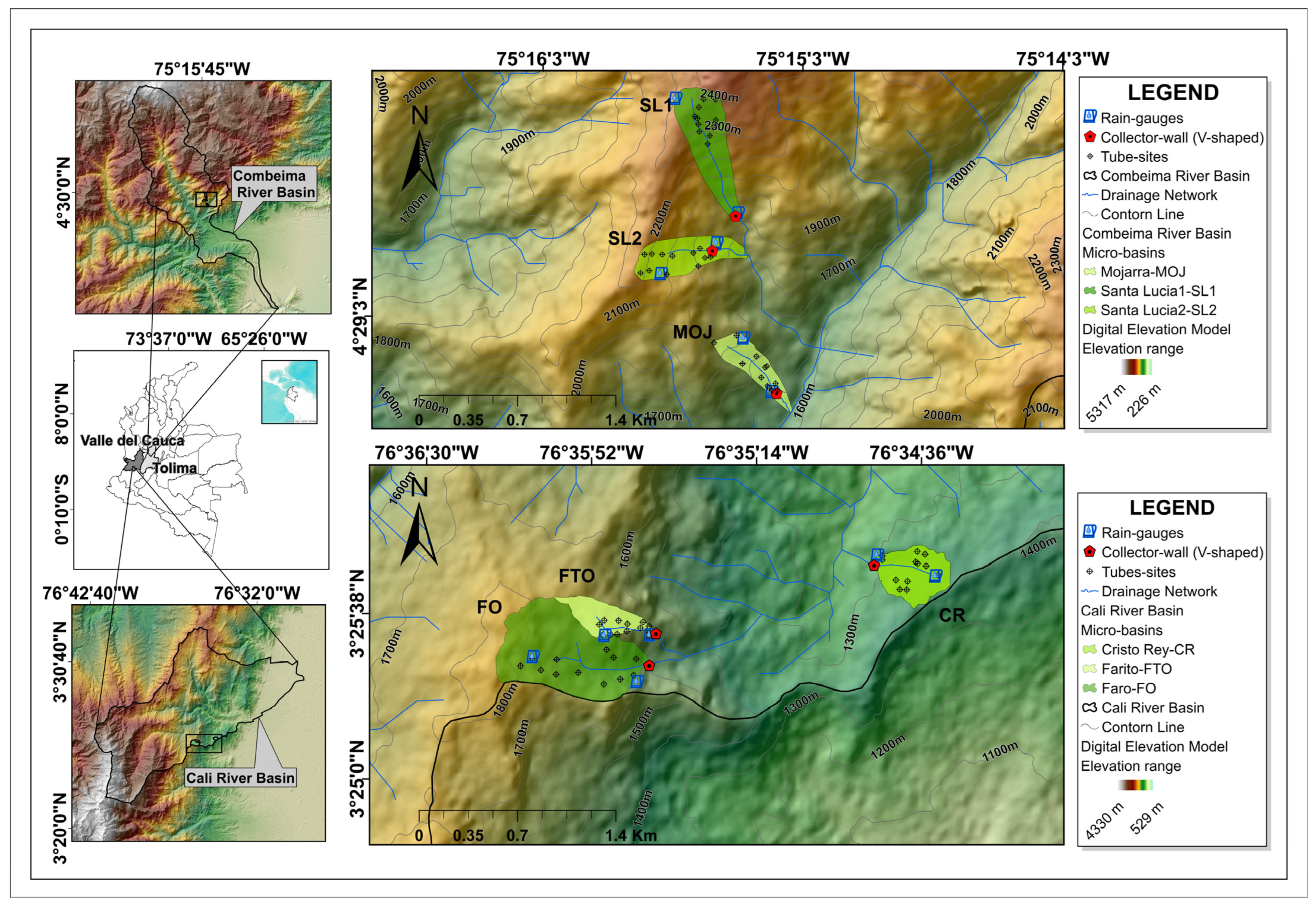
2.1. Study Area

This research was conducted in six experimental micro-watersheds (EMs) within the Combeima and Cali River basins, located in the Tolima and Valle del Cauca departments of the central Andean region of Colombia. The EMs, situated between 1250 m and 2350 m elevations, were categorized into three LULC classes: natural forest (NF), pasture (P), and coffee agroforestry system (AS-c). Figure 1 shows the distribution of the EMs (Santa Lucía 1 (SL1), Santa Lucía 2 (SL2), Mojarra (MOJ), Faro (FO), Farito (FTO), and Cristo Rey (CR)), their respective LULC. Figure 2 shows the LULC map for the study area and its surroundings, which is consulted on the official platform of the Institute of Hydrology, Meteorology and Environmental Studies (IDEAM) for the most recent year available in the open database (https://qrcd.org/63VD (accessed on 21 June 2024)). Similarly, for each MS, the images taken by the author for the comparison and verification of the state of LULC in the basins under study are shown. The instrumentation setup is shows in the Figure 3a–h.

The effective areas, average coordinates, and elevation ranges for each EM are listed in

Table 1. Area, coordinates, and altitudinal range of the experimental micro-watersheds (EMs) with their respective land use and land cover (LULC).

EMs (LULC)	Area (ha)	Coordinates		Altitudinal Range (m a.s.l.)
		North	West
Combeima River Basin
SL1 (NF)	22.8	4° 29.178′ N	75° 15.284′ W	1932–2322
		4° 29.443′ N	75° 15.306′ W
SL2 (P)	16.3	4° 29.294′ N	75° 15.657′ W	1928–2244
		4° 29.323′ N	75° 15.396′ W
MOJ (AS-c)	10.8	4° 28.972′ N	75° 15.270′ W	1590–1830
		4° 28.159′ N	75° 15.149′ W
Cali River Basin
FO (NF)	51.5	3° 25.468′ N	76° 36.086′ W	1484–1764
		3° 25.425′ N	76° 35.646′ W
CR (P)	16.5	3° 25.777′ N	76° 34.540′ W	1266–1386
		3° 25.818′ N	76° 34.782′ W
FTO (AS-c)	10.5	3° 25.591′ N	76° 35.837′ W	1524–1692
		3° 25.573′ N	76° 35.615′ W

Note: Santa Lucía 1 (SL1), Santa Lucía 2 (SL2), Mojarra (MOJ), Faro (FO), Farito (FTO), Cristo Rey (CR) natural forest (NF), pasture (P), and coffee agroforestry system (AS-c), meters above sea level (m a.s.l.).

. According to historical data on the main meteorological variables in the Combeima and Cali River basins, the mean annual temperature, respectively, is 20.8 °C and 25.4 °C; the mean annual evapotranspiration is 1038 and 1655 mm; the relative humidity is 70% and 79% per year; and the mean annual precipitation is 1887 mm and 1608 mm. According to the classification proposed by Holdridge, the life zones in the area range from tropical dry forests to premontane rainforests [27]. In the Combeima River basin, the physiographic landscape is characterized by deep valleys with steep mountain slopes, which range from 35° to 90° at altitudes between 1300 m and 5000 m [28]. The Cali River basin features a mountainous landscape with slopes between 14° and 26°.

Table 2. Record of average data of environmental variables associated with the experimental micro-watersheds (EMs).

EMs	Pp (mm)	Tm (°C)	RH (%)	S	PM	ST	LULC	Life Zone
Combeima River Basin
SL1	1578.1 ± 37.6	20.8	79.5	Steep	Granodiorite	Typic Eutrodepts	Natural forest (NF)	TP-mf
SL2	1730.6 ± 20.9	20.8	79.5				Pasture (P)
MOJ	2353.5 ± 23.0	20.8	79.5				Coffee agroforestry system (AS-c)
Cali River Basin
FO	1594.6 ± 71.1	25.4	70.6	Moderately Steep	Lateritic Basalt	Typic Haplustalfs	Natural forest (NF)	(T-df)
CR	1340 ± 55.4	25.4	70.6				Pasture (P)
FTO	1892.4 ± 62.5	25.4	70.6				Coffee agroforestry system (AS-c)

Note: EMs = experimental micro-watersheds, SL1 = Santa Lucía 1, SL2 = Santa Lucía 2, MOJ = Mojarra, FO = Faro, CR = Cristo Rey, FTO = Farito, NF = natural forest, P = pastures, AS-c = coffee agroforestry system; average precipitation (Pp), mean temperature (Tm), relative humidity (RH), slope (S), parental material (PM), soil type (ST), land use and land cover (LULC), tropical premontane moist forest (TP-mf), tropical dry forest (T-df).

shows the other environmental characteristics of the selected EMs, classified by the predominant LULC type.

2.2. TETIS Model

TETIS is a conceptual, balanced, and physical process-based model that is an excellent tool for simulating rainfall–runoff processes [20]. TETIS is a comprehensive model that simulates a range of water cycle processes and is particularly suited to arid climates, rainy areas, and regions with extreme winters. The model conceptualizes the hydrological cycle through the use of six vertically arranged tanks, with each tank representing a specific form of water storage [21]. These include snow storage, atmospheric storage, surface storage, gravitational storage, aquifer storage, and stream storage. The relationship between the different tanks is based on soil characteristics, including field capacity and saturated hydraulic conductivity of the soil and subsoil [29]. The principal advantages of distributed models are their capacity to represent the spatial variability of hydrological processes and to elucidate the dominant processes at the hillslope and river basin scale. The TETIS model estimates all hydrological flows occurring at the hillslope and watershed scale [30]. However, this approach requires a more detailed understanding and interpretation of the spatial and temporal variability of the HR, as well as needing more data, input information, and model parameters [19].

TETIS has been employed extensively in numerous tropical mountainous regions across watersheds in Colombia [20], Peru [13], Chile [31], Guatemala [14], Mexico [32], the United States of America [33], and Kenya [34]. Additionally, it has been utilized in basins within the Mediterranean context in Spain [35], as well as in other tropical and even-temperate regions, for the assessment of flooding behavior. Included is evaluating the behavior of floods, including flash and torrential floods, as well as changes in LULC and the influence of climate change on the HR. This is performed in specific evaluations of the relationship between vegetation and the management of areas and zones of the protection and conservation of natural ecosystems with water systems. In all of these applications, TETIS has served as a pivotal instrument for thematic and scientific analyses, as well as a foundation for decision-making and action plans related to the conservation and management of natural and modified ecosystems, integrated water resource management, risk management, and the planning and integrated management of watersheds.

Runoff (Q) calculation was performed using a spreadsheet that summarizes the TETIS model’s runoff estimation method. Daily precipitation data and annual mean temperature values obtained from the stations closest to the EMs were used. The initial storage conditions of the four tanks that make up the base structure and runoff generation support of the model were defined, supported by previous soil hydro-physical characterization. The timeframe considered for flow modeling was from April 2014 to November 2017.

2.3. Meteorological Data

Two rain gauges equipped with sensors for daily precipitation recording were installed in each EM, with a 5600-0625 tipping bucket device (Sutron Corp. (Sterling, VA, USA)) and a Rainlogger Edge 3002 rain sensor (Solinst, Georgetown, ON, USA). Atmospheric pressure changes were monitored with a Barologger Edge 3001 (Solinst). The average annual temperature was taken from meteorological stations provided by the Colombian Institute of Hydrology, Meteorology, and Environmental Studies (IDEAM, Bogotá, Colombia) near the study watersheds. Model parameters such as potential evapotranspiration (ETp) were estimated on this.

2.4. Observed Flow Data

A collector wall with a V-shaped spillway was constructed to collect all the flow that drained into the micro-watershed area. Level sensors were installed to calculate the flow rate, along with a limnimetric ruler. Levellogger Model 3001 sensors (Solinst) were used to synchronize and calculate the flow regime every 5 min. Gauging was carried out in each micro-basin using an OTT C2 Hydromet micromolinete, and volumetric gauging using gauging containers and stopwatches. For most of the investigation, gauging was conducted simultaneously and very close to the collecting walls with weirs due to low flow quantities (see Figure 3a–h).

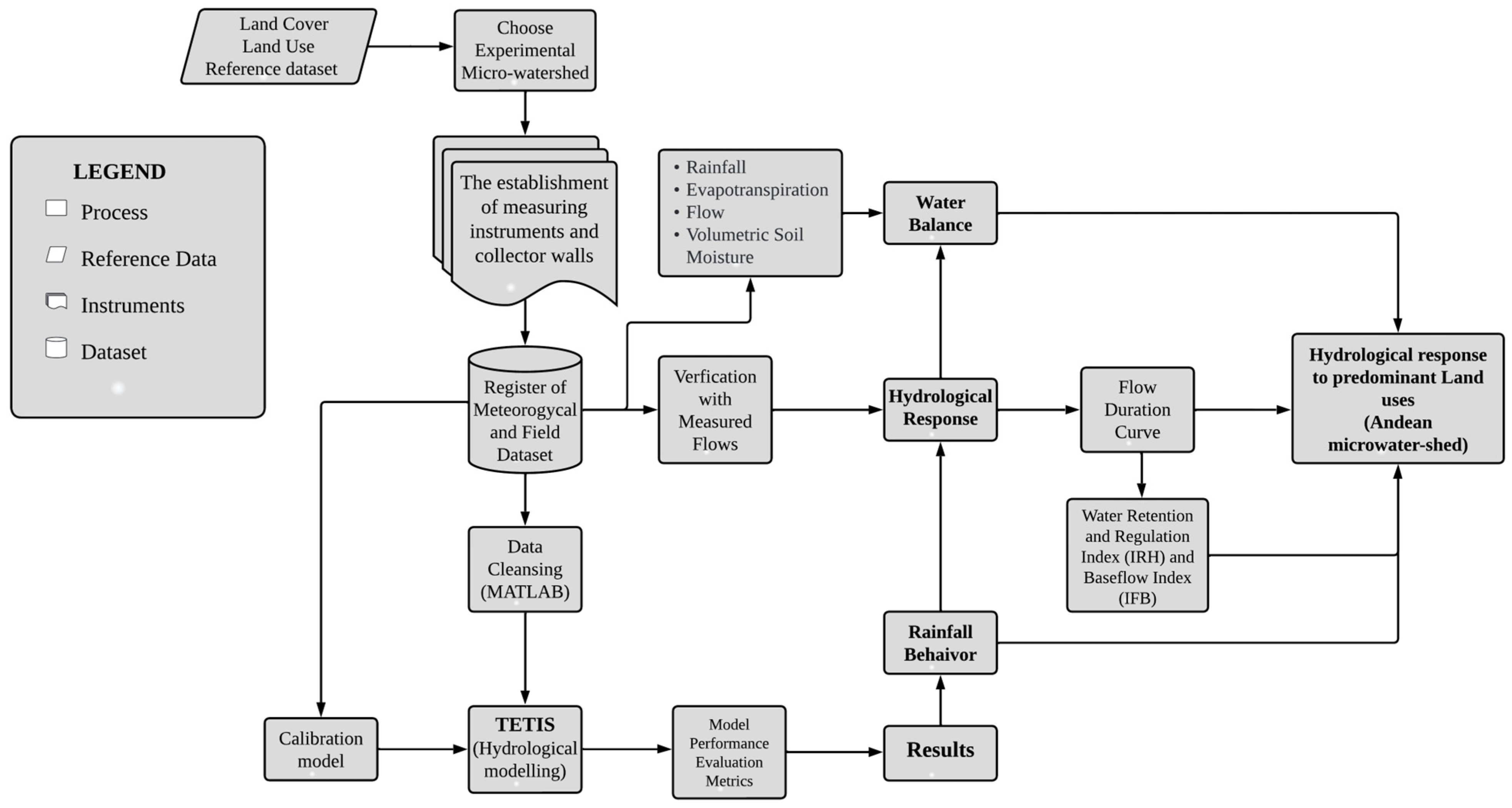
2.5. Data Processing and Analysis

The free software MATLAB version R20008a (MathWorks, Portola Valley, CA, USA) was used to process daily, hourly, and minute-to-minute rainfall data in order to characterize the rainfall regime and its space–time distribution. Excel spreadsheets were used to determine measures of central tendency of precipitation. Subsequently, runoff was calculated using a spreadsheet adapted from the TETIS model with input information that, given its conceptual structure and algorithmic basis, allowed for the automatic generation of simulated runoff.

2.5.1. Initial Conditions and Model Calibration Parameters

Initial storage conditions for the model’s four tanks were defined based on soil hydro-physical characteristics. Model parameters were iteratively adjusted to achieve physical consistency and the best fit between observed and simulated flows. Agreement was sought between the model-produced water volumes and those observed in each micro-basin. Gauging datasets from each EM were used to recalibrate the model, enhancing the accuracy of the predicted Q values (

Table 3. Parameters and initial conditions applied to the aggregated and simplified TETIS model, micro-basins, Combeima River basin and micro-basins, and Cali River basin.

Input Variables		Combeima River Basin			Cali River Basin			Reference Values
		Micro-Basins			Micro-Basins
		SL1	SL2	MOJ	FO	CR	FTO	Min	Max
Initial conditions	Capillary storage	70	60	70	60	60	80	25	100
	Surface water storage	0	0	0	0	0	0	0	0
	Upper gravitational Z storage	5	5	10	15	15	15	5	22
	Lower gravitational Z storage (aquifer)	120	150	100	150	100	200	120	600
Parameters	Capillary storage (mm/day)	180	160	160	180	160	160	50	200
	Top layer conductivity (mm/day)	26	18	22	24	20	26	7.5	30
	Bottom layer conductivity (mm/day)	8	8	6	4	7	6	2.5	10
	Underground losses (mm)	0	0	1	0	3	0	0	0
	Surface flow average residence time (days)	2	1	1.5	1.5	1.1	1.5	1	2
	Mean subsurface flow residence time (days)	15	10	10	15	5	10	2.5	10
	Baseflow average residence time (days)	150	150	150	200	120	150	50	200

).

2.5.2. Model Verification

As described above, the gauging datasets from each of the EMs were used to verify the TETIS model. The model’s accuracy and performance evaluation metrics were calculated to compare the results it generated with the datasets recorded by sensors and those obtained through conventional measurements.

2.5.3. Flow Duration Curves (FDCs)

FDCs are a tool used to indicate the distribution of the occurrence of flow values over time. The CDC represents the relationship between the magnitude of flow and the frequency or percentage of times on which this magnitude is equaled or exceeded, and it is used to characterize the long-term flow regime of a natural stream. To construct it, recorded flow values are ordered from highest to lowest and each flow value is assigned a probability of being exceeded (empirical Weibull probability function). Flow data are then plotted on the ordinate axis and the corresponding probability values are plotted on the abscissa axis [36,37].

$$PE\left(\%\right)={\displaystyle \frac{x_i}{\left(1+N\right)}}\ast 100$$

(1)

where

• PE (%) = probability of exceedance expressed as a percentage;
• x_i = position of data in descending order;
• N = total amount of data.

2.5.4. Water Retention and Regulation Index (IRH) and Baseflow Index (IFB)

The Moisture Retention and Regulation Index (IRH) and Base Flow Index (IFB) were calculated to explain soil moisture regulation and its impact on flow behavior. IRH was derived from the ratio between the volume below the mean flow line and the total volume under the FDCs. Higher IRH values indicate greater moisture retention and regulation. The IFB was calculated to quantify the contribution of base flow to total flow, using a method based on Nathan and McMahon [38] and Lim et al. [39], cited by Vásquez-Velásquez [40].

$$IRH={\displaystyle \frac{V_{qm}}{V_t}}$$

(2)

where

• IRH = Water Retention and Regulation Index;
• V_qm = Volume corresponding to the area below the mean flow line at FDCs;
• V_t = Total volume corresponding to the area under the FDCs.

$$q_t=\propto q_{t-1}+\left[{\displaystyle \frac{1+\propto }{2}}\right]\ast \left(Q_t-Q_{t-1}\right)$$

(3)

where

• $q_t$ = direct runoff flow filtered at time t;
• $q_{t-1}$ = direct runoff flow filtered at the previous time t − 1;
• α = filtration parameter (dimensionless);
• $Q_t$ = total flow at time t;
• $Q_{t-1}$ = total flow rate at time t − 1.

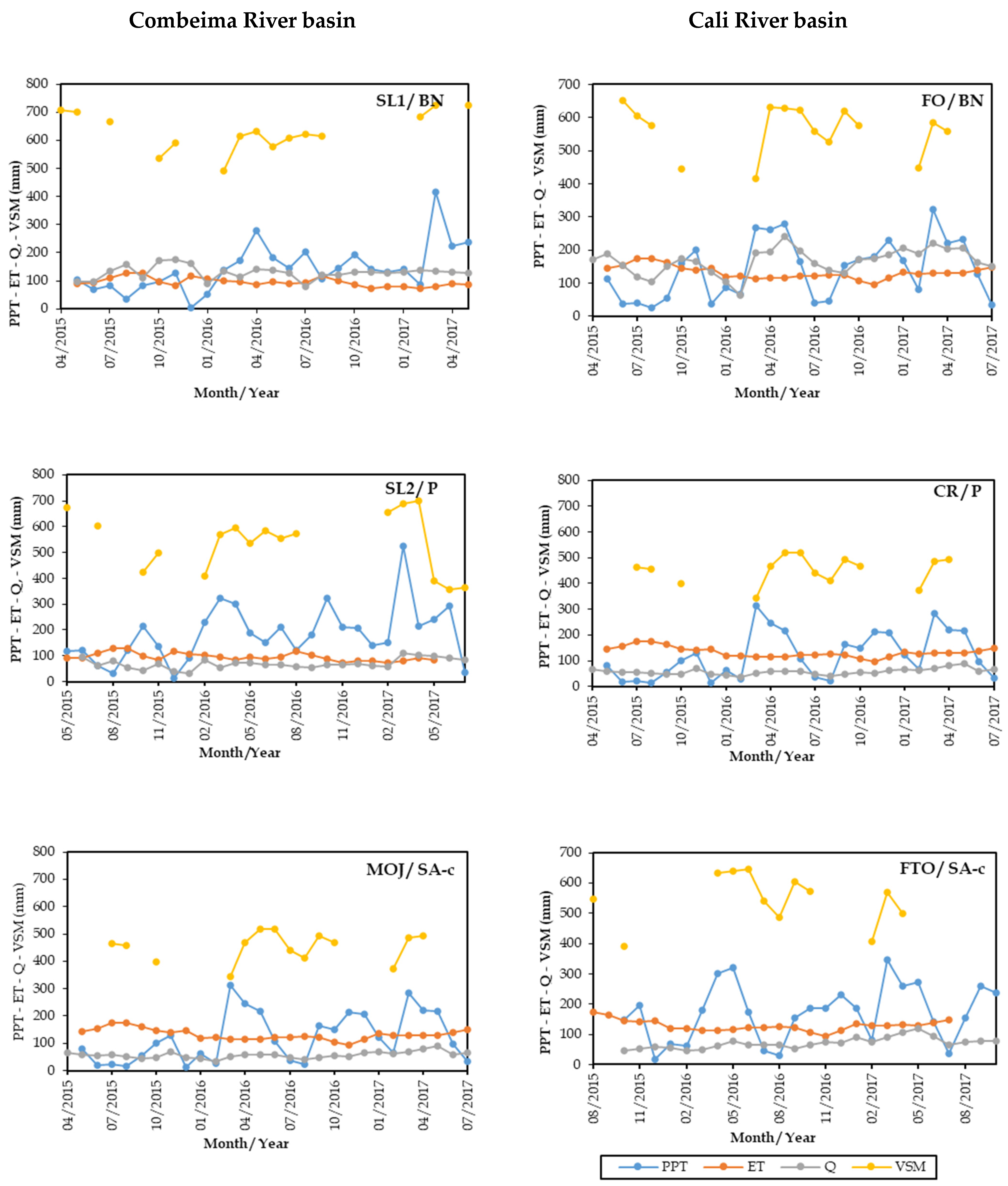
2.6. Water Balances at the Micro-Watershed Scale

In understanding the hydrologic response at the watershed scale, the rainfall–flow relationship, and the redistribution of rainfall in the context of the hydrologic cycle, the water balance and mass conservation equation (Equation (4)) has proven to be the fundamental conceptual and methodological resource for understanding, quantifying, and evaluating this relationship and balance.

$$ds/dt=P-\left(Q+ETR+D\right)$$

(4)

where

• P = Precipitation recorded (mm).
• Q = Flow recorded (mm).
• ETR = Actual evapotranspiration/estimated potential (mm).
• D = Recharge of subway storage. It may not be taken into account, since it is usually the smallest in the balance.
• ds/dt = Change in soil water storage (mm). It can be constant or not taken into account because it can be the same at the beginning and end of the balance.

Equation (4) can be expressed as

$$Q=\left(P-ET\right)\ast A$$

(5)

where

• A = watershed area (km²).

2.7. Model Performance Evaluation Metrics

The TETIS model’s performance was evaluated by comparing the correspondence of the simulated data output with the data observed in the field and establishing the statistical proximity between the actual and predicted data. The coefficient of determination (R²), root mean square error (RMSE), Nash Efficiency Coefficient (NSE), and Balance Percentage Error (BE) were used in this study. These statistical parameters are widely used to evaluate the performance of linear and nonlinear models [41].

R² describes the collinearity between observed and simulated Q data. R² can vary from 0 to 1; the closer its value is to 1, the lower the error variance, indicating concordance between the data [42].

$$R^2={\left\{{\displaystyle \frac{{{\displaystyle \sum }}_{i=1}^N\left(Oi-\overline{O}\right)\left(Pi-\overline{P}\right)}{{\left[{{\displaystyle \sum }}_{i=1}^N{(Oi-\overline{O})}^2\right]}^{0.5}\ast {\left[{{\displaystyle \sum }}_{i=1}^N{(Pi-\overline{P})}^2\right]}^{0.5} }}\right\}}^2$$

(6)

The RMSE quantifies the magnitude of the deviation between simulated and observed values. The range of values it can take is from 0 to infinity (positive). A value equal to 0 corresponds to a perfect fit, while larger values indicate a poorer fit.

$$RMSE=\sqrt{{\displaystyle \frac{{{\displaystyle \sum }}_{i=1}^{(N}{\left(Pi-Oi\right)}^2}{N}}}$$

(7)

The NSE is a statistical coefficient used to evaluate hydrologic models. It determines how accurately the model simulates data or how well the observed and simulated data fit linearly. It explains how much of the variability in observations is explained by the simulation. If the simulation is perfect, NSE = 1 [43,44].

$$NSE=1-\left[{\displaystyle \frac{{{\displaystyle \sum }}_{i=1}^N{\left(Oi-Pi\right)}^2}{{{\displaystyle \sum }}_{i=1}^N{\left(Oi-\overline{O}\right)}^2}}\right]$$

(8)

BE (%) describes the overall percentage error between the averages of the observed and simulated values. For Equations (6)–(9), the parameters for the calculation are defined as follows:

$$BE\left(\%\right)=\left[{\displaystyle \frac{\left(\overline{P}-\overline{O}\right)}{\overline{O}}}\right]\ast 100$$

(9)

where

• Oi = observed data;
• Pi = simulated data;
• $\overline{O}$ = average observed data;
• $\overline{P}$ = average simulated data;
• $N$ = total number of observations.

Figure 4 presents a flowchart that provides a summary of the methodological and implementation process that guided the development of this research.

3. Results and Discussion

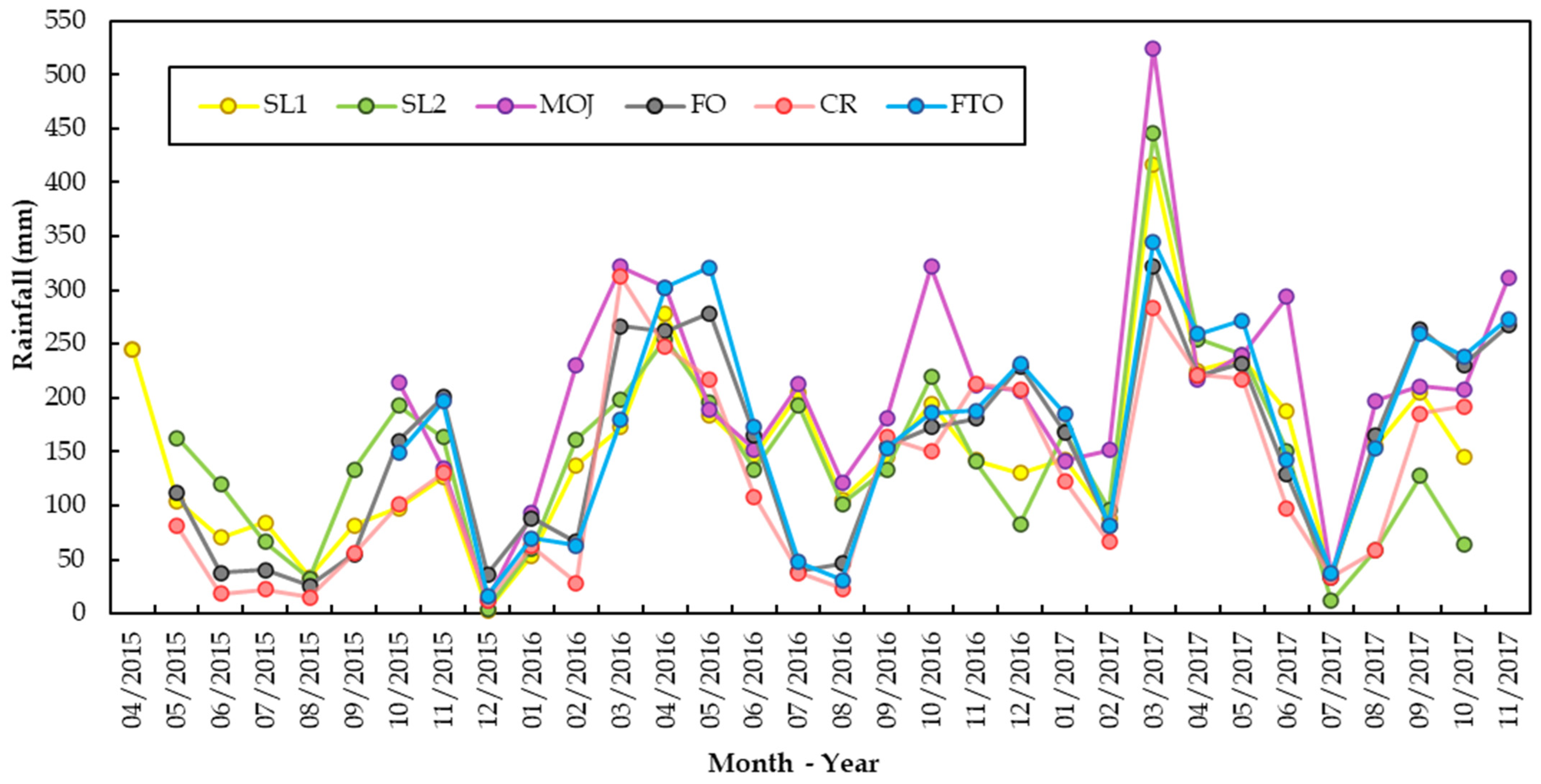
3.1. Precipitation Behavior

In the Combeima River basin, the SL1 (natural forest) micro-watershed presents the lowest precipitation values for the months of August (32.5 mm) and December (3 mm) of 2015 (the driest month of the entire study) as well as for July (11.9 mm) of 2017. The MOJ (coffee agroforestry system) micro-basin presents the highest rainfall values in March (322 mm) of 2016 and March (524.6 mm) of 2017 (the wettest month of the study period). Throughout the study period, no excessive rainfall periods or prolonged droughts were recorded in any of the Combeima micro-basins. In contrast, the Cali River micro-basins show more pronounced periods of drought, with dry periods in the months of June, July, August, and December 2015; January, February, July, and August 2016; and July and August 2017. The lowest rainfall in the CR (pasture) micro-basin occurred in August (15.4 mm) and December (12.5 mm) of 2015.

In the FTO micro-basin, the wettest periods were March (302.3 mm), April (302.3 mm), and May (321.1 mm) 2016, as well as March (345 mm) 2017 (Figure 5). The MOJ (230.8 mm) and CR (28.4 mm) micro-basins show a significant difference in rainfall for the month of February 2016. A similar phenomenon was observed in March 2017 (MOJ—524.6 mm, CR—283 mm). This difference is due to microclimatic and altitude factors [14,32]. The driest month of the entire study period was December 2015 (Combeima—3 mm, Cali—37 mm); July 2017 was also exceptionally dry (Combeima—12 mm, Cali—38 mm). In the Colombian Andes, precipitation shows a visible variability that, in principle, can be attributed mainly to the occurrence and interaction of macro- and mesoscale processes, including the ENSO phenomenon, microclimatic and orographic factors, and altitudinal gradients [45,46].

This behavior of the rainfall regime may be mainly related to the origin of the rains, essentially orographic, with the geomorphological variability and altitudinal gradients of the basins under study (many of these dynamics are typical of the central Andean context of Colombia), according to [47,48]. With dynamics related to microclimatic processes that can probably be associated to behaviors and manifestations of interactions between macroclimatic processes such as ENSO, mesoclimatic processes themselves of the orographic rain fronts and the presence and manifestation of some convective rain fronts that may be due to the integration of processes associated with these three scalar levels have been observed and detailed in the field in the area by our own experience and partly explain why the MOJ (SA-c) micro-basin presented in the Combeima River basin involves the highest rainfall regime with monthly values of up to 540 mm for the month of March 2017 [45,46,48].

3.2. Hydrological Response (Hydrological Modeling)

After applying the aggregated and adapted TETIS model [8,20,21],

Table 4. Area, average annual precipitation, and average daily, minimum, and maximum flows observed and simulated using the TETIS model by micro-basin.

EMs/LULC	Pm (mm/Year)	Qmdobs (L/s)	Qmdsim (L/s)	Qmindobs (L/s)	Qmindsim (L/s)	Qmaxdobs (L/s)	Qmaxdsim (L/s)
Cuenca Río Combeima
SL1/NF	1578.1 ± 37.62	6.85	6.26	1.18	2.6	41.31	41.59
SL2/P	1730.65 ± 20.86	5.37	4.79	0.02	2.14	43.5	69.8
MOJ/AS-c	2353.55 ± 23.05	2.51	2.79	0.04	0.42	16.46	26.38
Cuenca Río Cali
FO/NF	1594.65 ± 71.10	17.87	14.23	0.19	3.08	85.4	258.61
CR/P	1340 ± 55.37	1.54	2.02	0.1	0.15	35.87	57.15
FTO/AS-c	1892.45 ± 62.55	2.71	2.04	0.2	0.34	61.13	40.85

Note: Ems = experimental micro-watersheds, LULC = land use and land cover, Pm = mean annual precipitation, Qmdobs = observed mean daily flow, Qmdsim = simulated mean daily flow, Qmindobs = observed minimum daily flow, Qmindsim = simulated minimum daily flow, Qmaxdobs = observed maximum daily flow, Qmaxdsim = simulated maximum daily flow.

shows the flow rates estimated by this model and the values of the observed flows. The table shows that the average daily flow observed in SL1 (NF) was 6.85 L/s; in SL2 (P), 5.37 L/s; and in MOJ (AS-c), 2.51 L/s. These flows, in principle, correspond to their catchment and drainage areas. The higher hydrological yield in SL1 may be related to the type of forest cover, since fog can contribute to precipitation in low montane forests, as well as to the location of this micro-basin and its altitudinal gradient between 2100 and 2400 m a.s.l. According to Ramírez et al. [49], in some areas of the Colombian Orinoco, increases in hydrological response and higher mean daily flows in Andean montane forest micro-watersheds can be attributed to precipitation inputs in the form of fog, which is characteristic of the hydrological behavior of many areas of the equatorial Andean context with tropical montane forests. The table also shows a significant water yield due to the high mean annual precipitation in the La Mojarra micro-basin (MOJ).

The mean flows observed in the Cali River micro-watersheds were 17.87 L/s (FO), 1.54 L/s (CR), and 2.71 L/s (FTO). In FO, the flows were the highest due to the fact that this micro-basin has the greatest extension, which favors a greater contribution or concentration of surface flows (runoff) and most likely due to subsurface contributions. The latter may also be related to the type of forest cover where organic matter such as leaf litter and mulch contributes to greater water retention in the soil and may favor subsurface flow contributions [32,50]. In contrast, the lowest flows were observed in the CR micro-watershed. This is directly related to its drainage area, lower precipitation volume, possible percolation losses, and a higher level of evapotranspiration.

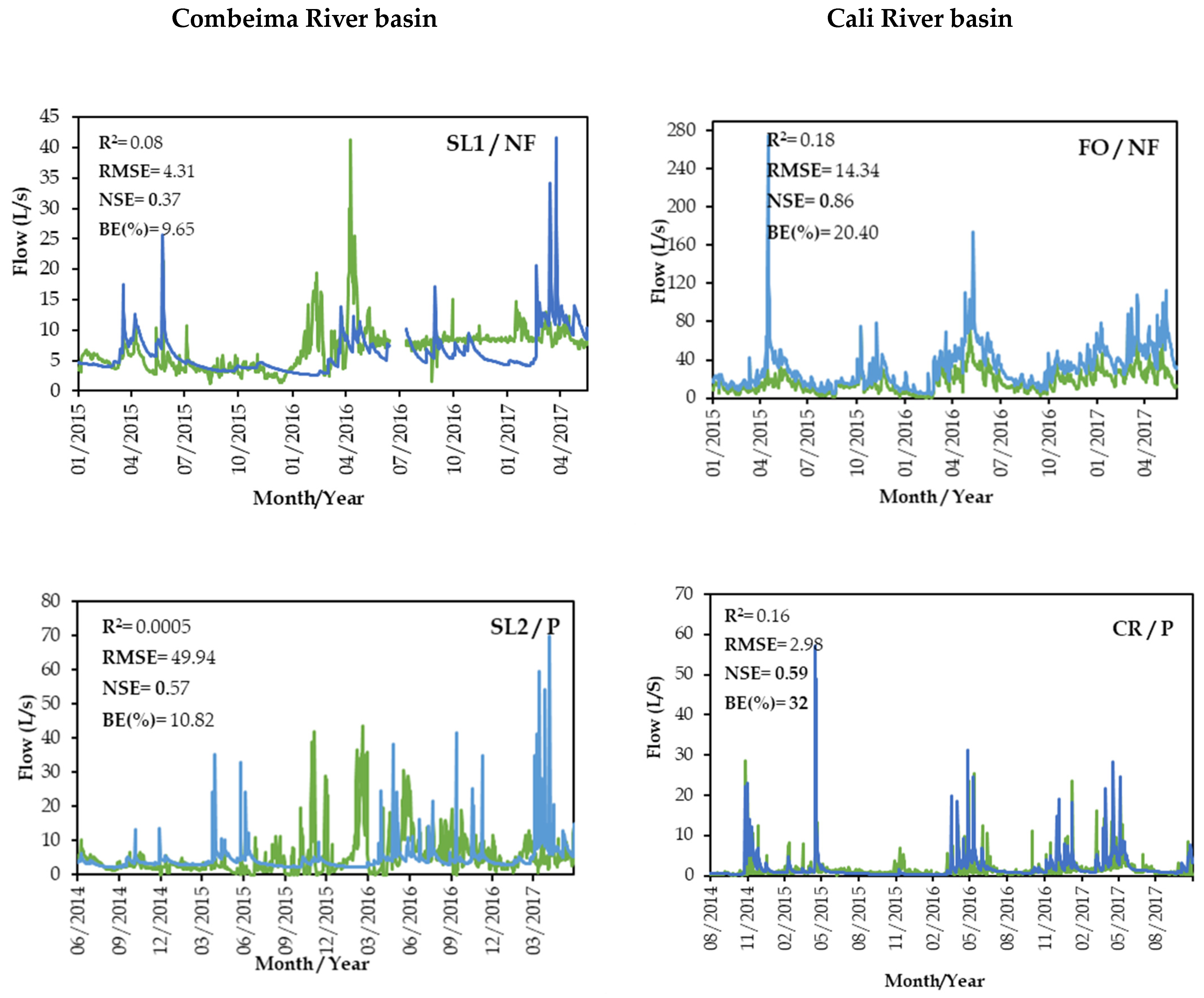
3.2.1. Model Calibration and Performance Evaluation

After calibrating and running the model, we evaluated the goodness of fit between the observed and simulated flows using the metric indicators selected for this study.

Table 5. Summary and recording of performance evaluation metrics of the calibrated and verified TETIS model for the study watersheds.

EMs/LULC	Tetis Model Performance Assessment Metrics
	Calibrated Model				Verified Model
	R2	RMSE	NSE	BE (%)	R2	RMSE	NSE	BE (%)
SL1/NF	0.08	4.31	0.37	9.65	0.89	0.77	0.89	1.84
SL2/P	0.0005	49.64	0.57	10.82	0.86	1.12	0.85	2.54
MOJ/AS-c	0.18	2.80	0.48	20.60	0.99	0.20	0.98	0.72
FO/NF	0.18	14.34	0.86	20.40	0.99	0.86	0.98	0.86
CR/P	0.16	2.98	0.59	32.00	0.78	0.34	0.73	3.22
FTO/AS-c	0.28	3.32	0.093	1.02	0.95	0.28	0.94	0.21

Note: Ems = experimental micro-watersheds, SL1 = Santa Lucía 1, SL2 = Santa Lucía 2, MOJ = Mojarra, FO = Faro, CR = Cristo Rey, FTO = Farito, NF = natural forest, LULC = land use and land cover, P = pastures, AS-c = coffee agroforestry system, R² = coefficient of linear determination, RMSE = root mean square error, NSE = Nash–Sutcliffe efficiency, BE = percent error in the balance.

summarizes the values obtained. Values for MOJ/AS-c were those that presented the best adjustment of de Combeima micro-basins with an RMSE of 2.80. SL1/NF and SL2/P had very low or poor concordance rates, with R² values of 0.08 and 0.0005, respectively. The NSE index showed a moderate trend, with values of 0.48 and 0.57 for micro-basins MOJ/AS-c and SL2/P.

In the Cali River basin, the natural forest micro-basin FO/NF showed the highest NSE value, at 0.86. FTO/AS-c had the lowest BE, at 1.02%. Additionally, this micro-basin and land use class had the best relative value of R². When comparing the observed and estimated flows in the six micro-watersheds and three investigated LULC classes, it is evident that MOJ/AS-c, despite having a BE of 20.60%, showed a moderate degree of NSE, at 0.48; an R² value of 0.18, which is not the lowest; and the best RMSE value of 2.80.

Figure 6 shows that for micro-basins SL1 (natural forest) and SL2 (pasture), the correspondence between the measured or observed flows and the flows simulated by the model was generally poor. However, there was some degree of correspondence for certain periods, such as from January 2015 to January 2016, from May to June and September to November 2016, and from March to May 2017 in SL1, except for the highest flows. In SL2, a similar phenomenon was also observed during several periods: June 2014–April 2015, April–May 2016, July–August 2016, and January, February, and May 2017. Barrientos et al. [31] applied TETIS in a study in the Chilean Andes; during the calibration period, the data showed an unsatisfactory fit between Qs and Qo, indicating that the hydrograph was correctly reproduced. However, the maximum simulated runoffs were often higher than the observed runoffs, and some Qo peaks were not reproduced. Additionally, the simulated runoffs during dry months were underestimated, with NSE values ranging from 30% to 60%.

3.2.2. Flow Duration Curves (FDCs) of the Calibrated Model

Figure 7 shows the degree of similarity between observed and simulated daily mean flows for the Combeima and Cali River micro-basins. The highest degree of similarity was observed in MOJ, followed by SL2 and SL1 in Combeima and by FTO, CR, and FO in Cali. Overall, the lowest degree of similarity was found in FO, followed by SL1. It is important to note that this analysis was essentially based on the careful observation of the behavior and trends of the respective CDFs and flow values in the respective quartiles. Thus, the daily flow regime in CR and FTO showed the least variation, with fluctuations between the first and third quartile values of 0.88 L/s and 1.81 L/s, respectively. In contrast, SL1 showed a much larger variation (6.09 L/s), between these two quartiles. This research confirms that there is an important relationship between a low variability in the flow duration curve (FDC) and the presence of subsurface storage processes that affect the flow, indicating that the flow tends to remain stable over time [50]. The daily flow regime and behavior at FO showed the greatest variation, which can be interpreted as being partly associated with steep slopes in this micro-basin.

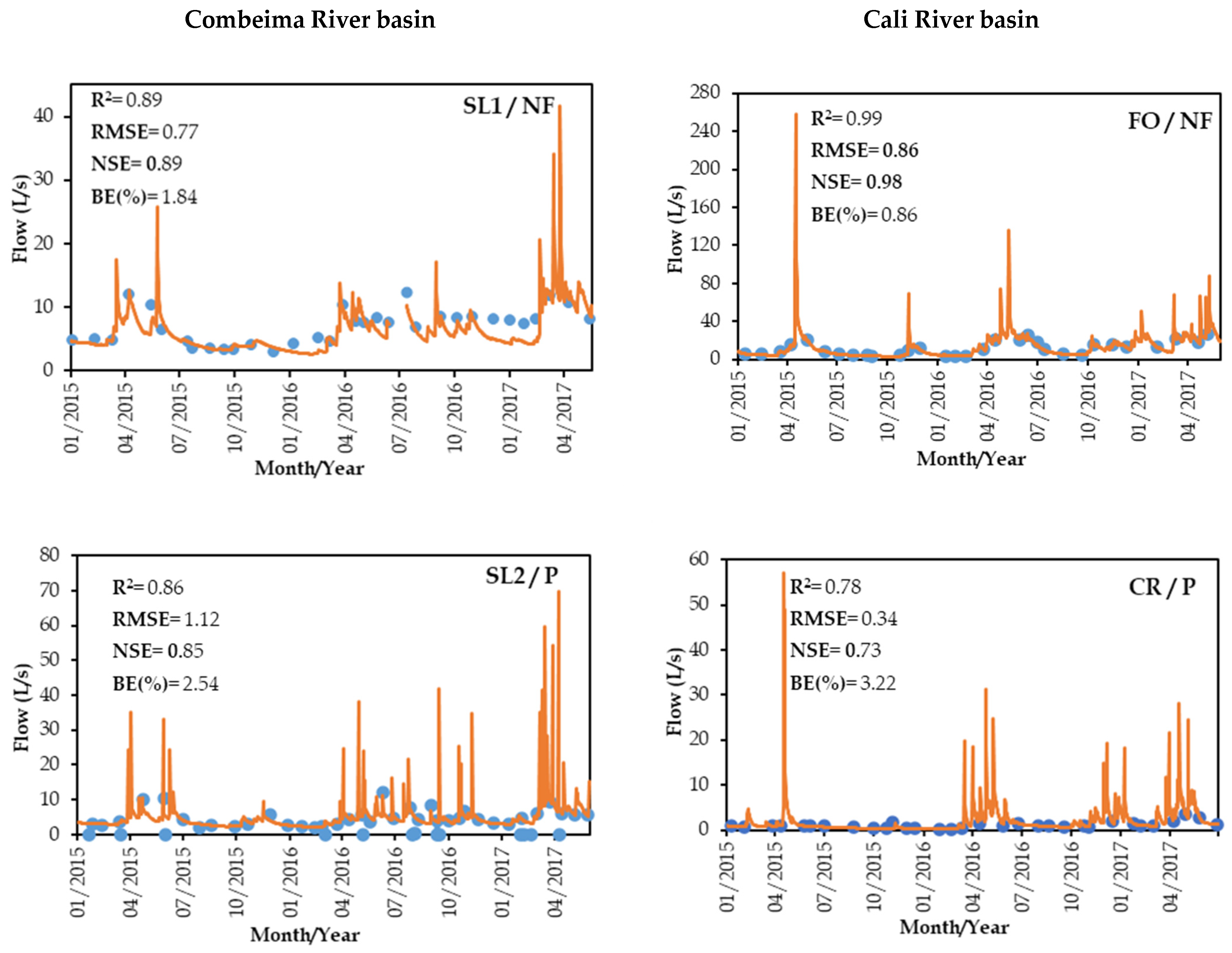
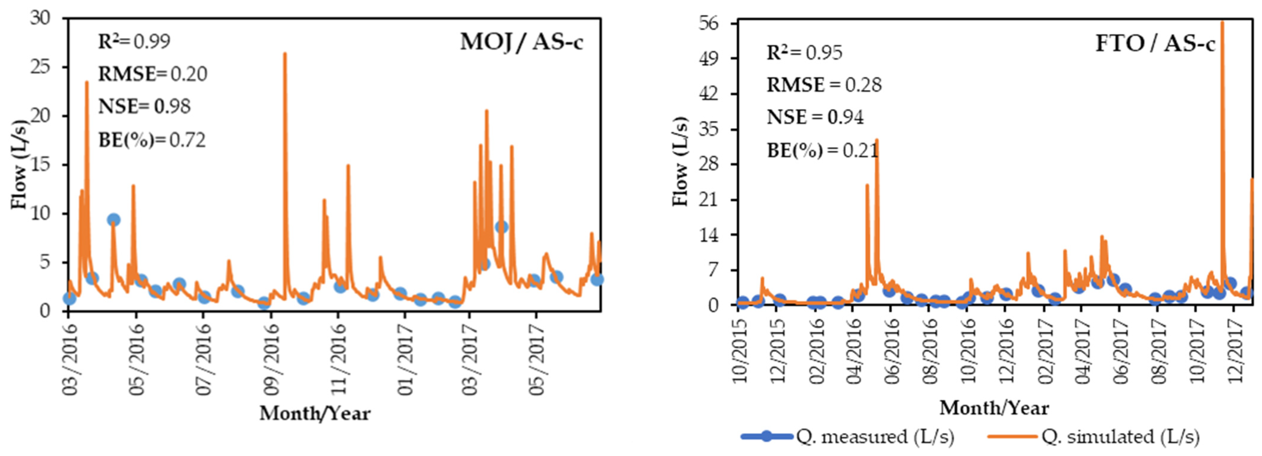
3.2.3. Model Performance Verification and Evaluation

After reviewing the initial calibration of the model, we set out to improve the level of fit and correspondence between the observed flows and those estimated by the model. With flow data obtained from volumetric gauging, we proceeded to verify and adjust the model, obtaining the results also presented in Table 5. The adjustment and recalibration or verification process significantly increased the similarity between the measured and simulated flows, which led to a substantial improvement in all the metric indicators of the model (R², RSME, NSE, and BE).

Improvements in R² were achieved in all LULC classes and micro-watersheds, with values ranging from 0.78 to 0.99. The highest values were achieved in MOJ/AS-c and FO/NF. The best RSME results of 0.28 and 0.20 were found in MOJ/AS-c and FTO-AS-c, respectively. MOJ/AS-c also proved to be the most efficient, with an NSE of 0.98, followed by FO/NF with 0.98; FO/NF-c, MOJ/AS-c, and FTO/AS-c had good or better BE values of 0.86, 0.72, and 0.21, respectively. In general, FTO/AS-c presented the most optimal results of the micro-watersheds of the agroforestry system with coffee. MOJ/AS-c presented the greatest improvement in the metric indicators of calibration, verification, and model fit in terms of R², RSME, and NSE indices, followed by FO/NF and FTO/AS-c, which also achieved very good metric R² and NSE results (Figure 8).

3.2.4. Flow Duration Curves (FDCs) of the Verified Model

Upon reviewing and adjusting the results of the FDCs for the Combeima and Cali River micro-basins, it was determined that the micro-basin with forest in FO (Cali River) presented the most significant variation in the distribution of measured and simulated flows, between the 20% percentile and the 62% exceedance. This is due to its pronounced and long stretch of FDC, which directly shows the transformation of precipitation into surface runoff. In this micro-watershed, the presence of shallow soils that can quickly become saturated, the high slopes, and the larger drainage area favor hortonian flows, which contribute to the formation of surface runoff. In contrast, the SL1 micro-watershed, also with forest, shows less variation in the percentile range (15–50%). This stability in terms of the flow regime is due to its smaller surface area and lower altitudinal gradient. Figure 9 shows the adjusted CDFs after model verification and adjustment.

Micro-basins with a less variable shape and slope tend to have a more stable flow regime due to contributions from storage and subsurface flows feeding the baseflow. Exceedance percentiles between 20% and 70% represent the transition from a higher to lower degree of stability, in the following order: SL2 (P) (flow fluctuation: 6.11–3.24 L/s); SL1 (NF) (flow fluctuation: 8.57–4.14 L/s); and MOJ (SA-C) (flow fluctuation: 3.30–1.45 L/s). The flow regime in the Combeima micro-watersheds was more stable, which can be attributed to the presence of deeper soils with low bulk density (high porosity) and high soil moisture retention (maximum moisture retention in SL2 was 64%). This facilitates an increase in subsurface and lateral flows, which contribute to baseflow, resulting in a better regulation of the watershed. Among all the micro-watersheds in the Cali River basin, CR exhibited the best regulation and stability, with flow fluctuations ranging from 1.51 to 0.61 L/s for the reference percentages.

Percentiles ranging from 70% to 99% exceedance are generally used to determine the minimum flow rates of a series [43,51]. For the SL1/NF micro-basin, these flow rates ranged from 4.45 L/s to 2.93 L/s (70.4–96.3% exceedance), while for SL2/P, they ranged from 3.24 L/s to 2.25 L/s (70.3–97.3%). For MOJ/AS-c, flow rates ranged from 1.54 L/s to 0.91 L/s (70–95%). Minimum flow values in the Cali River basin ranged from 5.41 L/s to 3.18 L/s (68.8–96.9% exceedance); in CR/P, from 0.61 L/s to 0.17 L/s (68.8–96.9%); and in FTO, from 0.98 L/s to 0.45 L/s (69–96.6%). The adjusted FDCs for MOJ/AS-c, FTO/AS-c, and FO/NF showed minimum values for periods between 3 and 4 months. Similarly, CR/P, SL2/P, and SL1/NF showed minimum values up to 8 months. This helps to explain the relationship of CDFs with permanent contributions to flows and with the maintenance of flows, since no critical drought periods or total absence of flow were found in any of the micro-watersheds and LULC types investigated.

3.3. Water/Hydrological Regulation Indexes

Natural forest micro-watersheds SL1 and FO exhibited the highest moisture regulation and retention indexes, ranging from 0.81 to 0.75 [52]. These values are linked to forest cover, which promotes a higher organic matter content in the soil, ensuring better water regulation and increasing soil moisture retention and permanence. This is also due to the moderate permeability and behavior observed in moisture retention curves [1]. The Moisture Retention and Regulation Index presented intermediate values in the MOJ and FTO micro-basins with the AS-c land use type due to the favorable effects of natural coffee agroforestry systems. The apparent density and moderate permeability conditions of this land use also favor the retention and permanence of moisture in the soil [1]. The CR pasture micro-basin exhibited the lowest moisture retention and regulation levels (0.62), likely due to anthropic intervention and soil compaction [1]. Figure 10 displays the IRH and IFB values.

In the Combeima River basin, SL1/NF had the highest IFB value (87.14%), indicating a significant contribution of subsurface and base flows to the total daily flow. On the other hand, SL2/P had the lowest IFB value (73.06%). In the Cali River basin, FO/NF had the highest IFB value (79.7%), while CR/pasture (77.3%) and FTO/AS-c (77.1%) had slightly lower values [40]. Considering the significance of the Base Flow Index (IFB) to the formation and contribution of subsurface flows and base flows, which essentially explain the minimum flows and their contribution to total flows or average daily flows, it is important to analyze the monthly IFB in each micro-basin and incorporate it into their respective series. The contribution of base flow to total flow in Combeima micro-basins varied throughout the study period. The highest values, ranging from 94.5% to 96%, were observed in SL1/NF in February and May 2015; July, November, and December 2016; and January and May 2017. In contrast, the lowest values were observed in SL2/P in December 2014, October 2015, April and September 2016, and November 2017, and ranged from 46.2% to 58.4%. In MOJ/AS-c, the IFB fluctuated between 70% and 90%, particularly in June, August, September, and November 2016, as well as in April 2017 (Figure 11).

The Cali River basin reported the highest IFBs, ranging from 89 to 92.6%, in FO/NF in December 2014, July 2016, and January 2017. In CR/P, the highest percentage values of IFB were also around 90%; in both FTO/AS-c and CR/P, the predominating values were between 70 and 80% for most months of the year. The lowest absolute values occurred in October 2014 and October 2015 and were 59.6% in CR and 60.7% in FO, respectively. According to Aboelnour et al. [53], the decrease in base flow observed in their micro-watershed study conducted at Walzem Creek may be attributed to the reduction in vegetation cover, particularly forest cover, and the increase in soil impermeability caused by soil compaction. This allows water to flow more quickly, resulting in greater surface runoff and a subsequent decrease in base flow in the main drainage network.

3.4. Water Balance

ET is a crucial component of water balance and represents the outflow (output) of water from a river basin’s natural hydrological system. In the WB equation, its quantification has typically been achieved through empirical methods and formulas [24,54,55,56,57]. This study estimated ET as either ETP or ETR (Potential or Real ET) using the methods of Garcia Lopez [24,58] based on climatological information from the Chapetón station for SL1, SL2, and MOJ in Combeima and from Margarita and Cañaveralejo for FO, FTO, and CR in Cali. ET was approximately 1038.61 mm yr-1 for the Combeima micro-basins and 1175 mm yr1 for the Cali micro-basins. These results were adjusted according to the predominant LULC, as reported by Ramírez-Builes et al. [59], Jaramillo-Robledo et al. [48], and Vásquez-Velásquez et al. [40]. Thus, water balance was estimated based on monthly records of precipitation (PPT), calculated evapotranspiration (ET), recorded streamflow (Q), and recorded volumetric soil moisture; the results are described below.

In SL1/NF, a marked tendency for ET to increase was observed in 2015 due to PPT. In 2016, this phenomenon was reversed, except for January and August, which are usually drier months in Colombia’s central Andean region. Regarding VSM, the lowest amounts of accumulated VSM were observed across the depth gradient between 50 and 160 cm [1] between October 2015 and February 2016. Thus, a significant correlation was observed between P dynamics and VSM behavior. Specifically, periods or months with higher PPT corresponded with higher VSM content. Increases in cumulative monthly P during October–November 2015, March–April 2016, and February–March 2017 directly reflected increases in cumulative VSM and implicitly in monthly Q sheets in the same periods. Regarding PPT and ET in SL2/P, there was a noticeable increase in ET from June to September 2015. However, in 2016, except for January and August, ET remained consistently lower than PPT. The same pattern was observed from January to May 2017. During the observed period, the recorded ET exceeded the recorded PPT. In 2016, there was also a greater variation in Q due to variation in PPT. In some months, there was a tendency for Q to increase with the increase in precipitation. Q became more stable between August 2016 and May 2017. However, despite very high accumulated rainfall in March 2017, there was no direct or noticeable impact on Q that month. It was observed that a decrease in P from May to June 2015 corresponded with a decrease in VSM and Q.

A correlation was found between PPT, VSM, and Q during August and October 2015. An increase in P led to an increase in VSM between October and November and to an increase in Q between September and November. During July–August 2016 and May–June 2017, a decrease in P resulted in a decrease in VSM, but not necessarily in a reduction in Q. It is important to note that the soil in this micro-basin and in the Combeima basin in general tends to have high moisture levels and can reach saturation levels despite having high soil bulk density (between 1.10 and 1.30 g·cm⁻³) and sandy loam textures. This is further supported by the significant amount of maintained VSM. The organic matter content of soil may contribute to its ability to retain and store moisture.

In MOJ/AS-c, from July to August 2015, PPT consistently exceeded ET. From January 2016 to May 2017, ET remained relatively stable. In September 2015 and August 2016, ET corresponded to almost 100% of PPT. Overall, the strongest correlation and direct relationship between PPT, VSM, and Q were observed from February to March 2017. There was also a direct relationship between P and VSM in both 2016 and 2017. Additionally, the soils maintained a high VSM content between March and August 2016, indicating a significant amount of VSM feeding the subsurface flows and base flows in this micro-basin. Figure 12 illustrates these behaviors in SL1, SL2, and MOJ in the Combeima watershed.

In FO/NF, the months with the lowest precipitation during the observed period were June, July, and August of 2015; July and August of 2016; and July of 2017. August 2015 was the driest month of the period. Conversely, the wettest months were March, April, and May of 2016; March 2017 was the wettest month of that year and of the entire observed period. Overall, 2015 was drier than 2016, and 2017 followed a similar pattern. The high recorded ET can be partly explained by the predominant El Niño conditions during 2015 and the first half of 2016 in the central–western part of the country. The lowest Qs were recorded in July and August 2015 and in February, August, and September 2016, with February 2016 being the driest. From October 2016 to May 2017, Q showed greater regularity, with consistently high values. From May to August 2015 and from May to July 2016, a direct decrease in Q was observed as P decreased. During the months of February–March 2016, an increase in PPT resulted in an increase in Q. It is important to note that, during the 15 months with observed VSM values, there was high moisture content for 11 months, which largely explains the availability of sufficient water to sustain losses or outflows in the form of ET in this basin and LULC class.

As for CR, in June, July, August, and December 2015, as well as in July and August 2016, PPT showed the lowest values during the observation period. December 2015 was the driest month, while March 2016 and March 2017 were the wettest. The year 2015 was significantly drier than 2016, and March to May 2016 and 2017 were the wettest months.

ET exhibited similar behavior to that of the FO/NF micro-basin due to the use of the same supporting information; a lower ET value occurred only in November 2016. Changes in P did not significantly affect changes in Q. However, a clear relationship was observed between PPT and VSM, where an increase in PPT from February to March 2016 resulted in an increase in VSM from March to April and May. The same pattern was observed in March 2017, when an increase in PPT led to an increase in VSM content. The monthly VSM contents accumulated in this micro-watershed were much lower than those found in the forest FO micro-watershed.

The driest months in FTO/AS-c were December 2015, July and August 2016, and July 2017, with December 2015 being the driest. The wettest months were March and April 2016 and March 2017. ET records were the same as in CR and FO, as they had the same calculation basis and were therefore high. Only November 2016 had a lower ET value. Q remained stable between October 2015 and February 2017. However, there was a significant increase in variation between March and October 2017. Overall, there was little correlation between PPT and Q, except for a slight increase in Q from April to May 2016 due to the monthly accumulated PPT from February to April of that year. Additionally, accumulated PPT from February to March 2017 had a more noticeable impact on the increase in Q during the months of March to May of that year. Generally, in this micro-basin, there was a direct relationship between the precipitation accumulated between February and March 2017 and a high content of suspended sediment, which in turn led to an increase in water discharge.

In general, the water balances for the six micro-watersheds and respective LULC indicate that, due to the soil’s high moisture content throughout the study period, the moisture retention curves and the percentages or saturation contents deduced from them [1] can be attributed to the soil’s permanent moisture content. Notwithstanding the fluctuations in precipitation and the persistent output of the evapotranspiration system, the soil consistently maintains a sufficient moisture content to sustain subsurface and base flows, thereby ensuring the persistence of minimum flows as indicated by the Base Flow Index.

4. Conclusions

The Combeima River basin exhibited a higher precipitation level than the Cali River basin, with the MOJ/P micro-basin displaying a notably higher average annual value compared to the other micro-basins and land uses under investigation. In this basin and micro-basin, it is hypothesized that the higher precipitation may be attributed to the interaction of macroclimatic dynamics associated with the El Niño–Southern Oscillation (ENSO) phenomenon, to the dynamics and behavior of the predominant orographic rain fronts in the central Colombian Andean context, and at certain times to convective rain fronts resulting from very focused orographic and microclimatic interactions and processes.

The natural forest land cover had the highest average daily flows, reaching 6.85 L/s in SL1/NF in the Combeima River basin and 17.87 L/s 644 in FO/NF in the Cali River basin. In general, flow rates were influenced by the basin area and drainage network, to a greater extent, and the type of natural forest cover. The organic matter produced by the forest cover, mainly leaf litter, promotes the formation and persistence of subsurface flows. These, along with surface runoff, contribute to the overall flow. Another indication of this behavior and its contribution to flow is explained by the higher moisture retention and regulation values for this land cover. The IRH showed values of 0.81 in SL1/NF and 0.75 650 in FO/NF, and the two micro-watersheds also presented high and good IFB values, at 651 87.1% and 79.7%, respectively.

After calibrating and evaluating the goodness of fit of TETIS with respect to the observed and simulated flows using the metric indicators R², RMSE, NSE%, and BE%, and interpreting the TDC for the six micro-basins and LULC investigated (NF, P, and AS-c), it was found that the MOJ/AS-c micro-basin had a moderate NSE of 0.48; an R² of 0.18, which can be considered good; and the best RMSE of 2.80. In addition, it should be noted that the BE (20%) was not low. After model verification, the R² value improved to 0.99, and the RSME improved to 0.28 and the NSE to 0.98. FO/NF and FTO/AS-c also presented very good R² and NSE values. It is important to note that all evaluations were objective and free of bias.

Based on the water balances carried out for the six micro-watersheds and respective LULC, despite some periods of very little rain, and the permanent output of the evapotranspiration system, there is always sufficient stock or volume of moisture in the soil that feeds the subsurface flows and base flows that guarantee the permanence of the minimum flows evidenced by a high Base Flow Index.

The findings of this study offer significant insights into the hydrological response, a product of hydrological and eco-hydrological interactions, when viewed through a systemic lens. Similarly, the findings contribute to the development of a framework for the integrated management of forest vegetation cover and land uses, as well as for the integrated planning of watersheds and territories.

In future research along these lines, it is deemed crucial to progress in instrumentation and monitoring to attain a more profound understanding of the behavior of variables and processes that integrate surface flows, subsurface flows, base flow, and groundwater flows at the scale of small- and medium-sized watersheds.

Furthermore, it is deemed strategic for future research to incorporate variables and processes pertaining to forest hydrology, including interception, flows through the canopy, the hydraulic architecture of species and ecosystems, stomatal conductance, and sap flow, among others.

References

1. Garzón-Sanchez, H.; Loaiza-Usuga, J.C.; Veléz-Upégui, J.I. Soil Moisture Behavior in Relation to Topography and Land Use for Two Andean Colombian Catchments. Water 2021, 13, 1448. [Google Scholar] [CrossRef]
2. Guo, X.; Fu, Q.; Hang, Y.; Lu, H.; Gao, F.; Si, J. Spatial Variability of Soil Moisture in Relation to Land Use Types and Topographic Features on Hillslopes in the Black Soil (Mollisols) Area of Northeast China. Sustainability 2020, 12, 3552. [Google Scholar] [CrossRef]
3. Dunne, T. Field Studies of Hillslope Flow Processes. 1978. Available online: https://www.researchgate.net/publication/243780862 (accessed on 19 October 2023).
4. Bruijnzeel, L.A. Hydrological functions of tropical forests: Not seeing the soil for the trees? Agric. Ecosyst. Environ. 2004, 104, 185–228. [Google Scholar] [CrossRef]
5. Llorens, P.; Latron, J.; Gallart, F. Dinámica espacio-temporal de la humedad del suelo en un área de montaña mediterránea. Cuencas experimentales de vallcebre (alto llobregat). Estud. Zona Satur. Suelo 2003, 6, 71–76. [Google Scholar]
6. Gusev, Y.; Busarova, O.Y.; Nasonova, O. Modelling Soil Water Dynamics and Evapotranspiration for Heterogeneous Surfaces of the Steppe and Forest-Steppe Zones on a Regional Scale. J. Hydrol. 1998, 206, 281–297. [Google Scholar] [CrossRef]
7. Piñol, J.; Lledó, M.J.R.; Escarré, A. Hydrological balance of two Mediterranean forested catchments (Prades, northeast Spain). Hydrol. Sci. J. -J. Des Sci. Hydrol. 1991, 36, 95–107. [Google Scholar] [CrossRef]
8. Medici, C.; Butturini, A.; Bernal, S.; Vázquez, E.; Sabater, F.; Vélez, J.I.; Francés, F. Modelling the non-linear hydrological behaviour of a small Mediterranean forested catchment. Hydrol. Process. 2008, 22, 3814–3828. [Google Scholar] [CrossRef]
9. Uber, M.; Vandervaere, J.-P.; Zin, I.; Braud, I.; Heistermann, M.; Legoût, C.; Molinié, G.; Nord, G. How does initial soil moisture influence the hydrological response? A case study from southern France. Hydrol. Earth Syst. Sci. 2018, 22, 6127–6146. [Google Scholar] [CrossRef]
10. Hörmann, G.; Horn, A.; Fohrer, N. The evaluation of land-use options in mesoscale catchments: Prospects and limitations of eco-hydrological models. Ecol. Model. 2005, 187, 3–14. [Google Scholar] [CrossRef]
11. Elfert, S.; Bormann, H. Simulated impact of past and possible future land use changes on the hydrological response of the Northern German lowland ‘Hunte’ catchment. J. Hydrol. 2010, 383, 245–255. [Google Scholar] [CrossRef]
12. Sidle, R.C.; Gomi, T.; Loaiza Usuga, J.C.; Jarihani, B. Hydrogeomorphic processes and scaling issues in the continuum from soil pedons to catchments. Earth-Sci. Rev. 2017, 175, 75–96. [Google Scholar] [CrossRef]
13. Meléndez Saldaña, D.; Ramos-Fernández, L.; Velásquez Bejarano, T.; Altamirano Gutiérrez, L. Simulación con un modelo hidrológico distribuido de tipo conceptual a escala diaria en una cuenca semiárida del río Lurín, Perú. Idesia 2021, 39, 17–26. [Google Scholar] [CrossRef]
14. Morales-de la Cruz, M.; Francés, F. Hydrological modelling of the “Sierra de las Minas” in Guatemala, by using a conceptual distributed model and considering the lack of data. In Geo-Environment and Landscape Evolution III; WIT Press: Southampton, UK, 2008; pp. 97–106. [Google Scholar] [CrossRef]
15. Song, S.; Wang, W. Impacts of Antecedent Soil moisture on the Rainfall–Runoff Transformation Process Based on High-Resolution Observations in Soil Tank Experiments. Water 2019, 11, 296. [Google Scholar] [CrossRef]
16. Bergström, S.; Graham, L.P. Abstract to “On the scale problem in hydrological modelling” [Journal of Hydrology 211 (1998) 253 265]. J. Hydrol. 1999, 217, 284. [Google Scholar] [CrossRef]
17. Hundecha, Y.; Bárdossy, A. Modeling of the effect of land use changes on the runoff generation of a river basin through parameter regionalization of a watershed model. J. Hydrol. 2004, 292, 281–295. [Google Scholar] [CrossRef]
18. Meijerink, A.M.J.; de Brouwer, J.A.M.; Mannaerts, C.M.; Valenzuela, C.R. Introduction to the Use of Geographic Information Systems for Practical Hydrology: IHP—IV M 2.3; ITC Publication; International Institute for Geo-Information Science and Earth Observation: Enschede, The Netherlands, 1994; Volume 23. [Google Scholar]
19. Velez, U.J.I. Desarrollo de un Modelo Hidrológico Conceptual y Distribuido Orientado a la Simulación de las Crecidas. Ph.D. Thesis, Universidad Politécnica de Valéncia, Valencia, Spain, 2001. [Google Scholar]
20. Velez, J.J.; Francés, F. Calibración Automática de Las Condiciones Iniciales de Humedad Para Mejorar La Predicción de Eventos de Crecida. 2008. Available online: https://www.researchgate.net/publication/236792187 (accessed on 26 February 2024).
21. Velez, J.; Velez, J.; Francés, F. Modelo distribuido para la simulación hidrológica de crecidas en grandes cuencas. In Proceedings of the XX Congreso Latinoamericano de Hidráulica, Havana, Cuba, 1–5 October 2002. [Google Scholar]
22. Kite, G.W.; Kouwen, N. Watershed modeling using land classifications. Water Resour. Res. 1992, 28, 3193–3200. [Google Scholar] [CrossRef]
23. Mendoza, M.; Bocco, G.; Bravo, M. Modelamiento hidrológico espacialmente distribuido: Una revisión de sus componentes, niveles de integración e implicaciones en la estimación de procesos hidrológicos en cuencas no instrumentadas. Investig. Geogr. 2001, 47, 929. [Google Scholar] [CrossRef]
24. Thornthwaite, C.W.; Mather, J.R. The Water Balance; Publications in Climatology: Centerton, NJ, USA, 1955. [Google Scholar]
25. Dunne, T.; Leopold, L.B. Water in Environmental Planning; Macmillan: New York, NY, USA, 1978. [Google Scholar]
26. Brutsaert, W. Hydrology—An Introduction; Cambridge University Press: Cambridge, UK, 2005. [Google Scholar] [CrossRef]
27. Holdridge, L. LIFE ZONE ECOLOGY with Photographic Supplement Prepared; Tropical Science Center: San José, Costa Rica, 1967. [Google Scholar]
28. Cuéllar-Cárdenas, A.M.; López-Isaza, A.J.; Carrillo-Lombana, E.J.; Ibáñez-Almeida, D.G.; Sandoval-Ramírez, J.H.; Osorio-Naranjo, J.A. Control de la actividad tectónica sobre los procesos de erosión remontante: El caso de la cuenca del río combeima, cordillera central, colombia tectonic activity control over the headward erosion process: The combeima river basin case, central mountain range, colombia. Bol. Geol. 2014, 36, 37–56. [Google Scholar]
29. Vélez Upegui, J.J.; Orozco Alzate, M.; Duque Méndez, N.D.; Aristizábal Zuluaga, B.H. Entendimiento de Fenómenos Ambientales Mediante Análisis de Datos; Universidad Nacional de Colombia: Manizales, Colombia, 2015. [Google Scholar]
30. Puricelli, M.; Francés, F.; Velez, J.J.; Unzu, F.L.; Vélez, J.J.; Puricelli, M.; Francés, F. Parameter extrapolation to ungauged basins with a hydrological distributed model in a regional framework Hydrology and Earth System Sciences Parameter extrapolation to ungauged basins with a hydrological distributed model in a regional framework. Hydrol. Earth Syst. Sci. 2009, 13, 229–246. [Google Scholar] [CrossRef]
31. Barrientos, G.; Herrero, A.; Iroumé, A.; Mardones, O.; Batalla, R.J. Modelling the effects of changes in forest cover and climate on hydrology of headwater catchments in South-Central Chile. Water 2020, 12, 1828. [Google Scholar] [CrossRef]
32. Molina Hernández, L.J.; Orozco Medina, I.; Farfán Gutiérrez, M.; Delgado Galván, X.; Mora Rodríguez, J.D.J. Evaluación del Efecto del Cambio de uso de Suelo Sobre la Disponibilidad Hídrica de las Fuentes: Superficial y Subterránea, Usando Como caso de Estudio la Cuenca del río Turbio en Guanajuato; Universidad de Guanajuato: Guanajuato, Mexico, 2018; Volume 4. [Google Scholar]
33. Quintero, F.; Velásquez, N. Implementation of TETIS Hydrologic Model into the Hillslope Link Model Framework. Water 2022, 14, 2610. [Google Scholar] [CrossRef]
34. Ruiz-Pérez, G.; Koch, J.; Manfreda, S.; Caylor, K.; Francés, F. Calibration of a parsimonious distributed ecohydrological daily model in a data-scarce basin by exclusively using the spatio-temporal variation of NDVI. Hydrol. Earth Syst. Sci. 2017, 21, 6235–6251. [Google Scholar] [CrossRef]
35. Fernández-Rodríguez, J.M.; Miralles-Rivera, M.C.; Álvarez-Álvarez, E. Modelización hidrológica de la cuenca alta del río Nalón (Asturias) para la determinación de recurso disponible destinado al abastecimiento de agua potable. Ing. Agua 2022, 26, 125–138. [Google Scholar] [CrossRef]
36. Gallego Arias, S.; Carvajal Serna, L.F. Regionalización de curvas de duración de caudales en el Departamento de Antioquia-Colombia. Rev. EIA 2017, 14, 21–30. [Google Scholar] [CrossRef]
37. Gaviria, C.J.; Carvajal-Serna, L.F. Determinación de la variabilidad de la curva de duración de caudales por efectos no estacionarios en Colombia. Ing. Agua 2020, 24, 269. [Google Scholar] [CrossRef]
38. Nathan, R.J.; McMahon, T.A. Evaluation of automated techniques for base flow and recession analyses. Water Resour. Res. 1990, 26, 1465–1473. [Google Scholar] [CrossRef]
39. Lim, K.; Engel, B.; Tang, Z.; Choi, J.; Kim, K.; Muthukrishnan, S.; Tripathy, D. Automated web GIS based hydrograph analysis tool, WHAT. JAWRA J. Am. Water Resour. Assoc. 2005, 41, 1407–1416. [Google Scholar] [CrossRef]
40. Vásquez-Velásquez, G. Headwaters Deforestation for Cattle Pastures in the Andes of Colombia and Its Implications for Soils Properties and Hydrological Dynamic. Open J. For. 2016, 6, 337–347. [Google Scholar] [CrossRef]
41. Shigute, M.; Alamirew, T.; Abebe, A.; Ndehedehe, C.E.; Kassahun, H.T. Understanding Hydrological Processes under Land Use Land Cover Change in the Upper Genale River Basin, Ethiopia. Water 2022, 14, 3881. [Google Scholar] [CrossRef]
42. Moriasi, D.; Arnold, J.; Van Liew, M.; Bingner, R.; Harmel, R.D.; Veith, T. Model Evaluation Guidelines for Systematic Quantification of Accuracy in Watershed Simulations. Trans. ASABE 2007, 50, 885–900. [Google Scholar] [CrossRef]
43. Nash, J.E.; Sutcliffe, J.V. River flow forecasting through conceptual models part I—A discussion of principles. J. Hydrol. 1970, 10, 282–290. [Google Scholar] [CrossRef]
44. Camila, L.; Murcia, C. Ajuste y validación del modelo precipitación–escorrentía gr2m aplicado a la subcuenca nevado. Ph.D. Thesis, Universidad Santo Tomás, Barranquilla, Colombia, 2018. [Google Scholar]
45. Montealegre, J.E. Estudio de la Variabilidad Climática de la Precipitación en Colombia Asociada a Procesos Oceánicos y Atmosféricos de Meso y Gran Escala. IDEAM: Bogotá, Colombia, 2009. [Google Scholar]
46. Ruiz, D.; Martinson, D.G.; Vergara, W. Trends, stability and stress in the Colombian Central Andes. Clim. Change 2012, 112, 717–732. [Google Scholar] [CrossRef]
47. Hoyos, N.; Waylen, P.R.; Jaramillo, Á. Seasonal and spatial patterns of erosivity in a tropical watershed of the Colombian Andes. J. Hydrol. 2005, 314, 177–191. [Google Scholar] [CrossRef]
48. Jaramillo-Robledo, A.; Chaves-Córdoba, B. Distribución de la precipitación en colombia analizada mediante conglomeración estadística. Cenicafé 2000, 51, 102–113. [Google Scholar]
49. Ramírez, B.H.; Teuling, A.J.; Ganzeveld, L.; Hegger, Z.; Leemans, R. Tropical Montane Cloud Forests: Hydrometeorological variability in three neighbouring catchments with different forest cover. J. Hydrol. 2017, 552, 151–167. [Google Scholar] [CrossRef]
50. Berbesí-Jaimes, A.; Loaiza-Usuga, J.C.; Casamitjana-Causa, M.; Cardona-Gallo, S.; Correa, G.A. Hydrogeochemical Nitrogenous Behaviour in an Andean Agricultural Basin. In Water Perspectives in Emerging Countries; Araruna, J., Jr., Granato, A., Julia Stuchi, R.S., Eds.; Cuvillier Verlag: Göttingen, Germany, 2019. [Google Scholar]
51. Barrientos, G.; Iroumé, A. The effects of topography and forest management on water storage in catchments in south-central Chile. Hydrol. Process. 2018, 32, 3225–3240. [Google Scholar] [CrossRef]
52. IDEAM. Estudio Nacional del Agua 2014; Publicación Aprobada por el IDEAM, Bogotá D.C., Colombia—Distribución Gratuita. 2015; Instituto de Hidrología, Meteorología y Estudios Ambientales—IDEAM: Bogotá, Colombia, 2014. [Google Scholar]
53. Aboelnour, M.; Gitau, M.W.; Engel, B.A. A comparison of streamflow and baseflow responses to land-use change and the variation in climate parameters using SWAT. Water 2020, 12, 191. [Google Scholar] [CrossRef]
54. Turc, L. Water requirements assessment of irrigation, potential evapotranspiration: Simplified and updated climatic formula. Ann. Agron. 1961, 12, 13–49. [Google Scholar]
55. Monteith, J.L. Evaporation from Land Surfaces: Progress in Analysis and Prediction since 1948; American Society of Agricultural Engineers: St. Joseph, MI, USA, 1985. [Google Scholar]
56. Penman, L.H. Natural evaporation from open water, bare soil and grass. Proc. R. Soc. Lond. Ser. A Math. Phys. Sci. 1948, 193, 120–145. [Google Scholar] [CrossRef]
57. Budyko, M.I. Climate and Life; Academic Press: Cambridge, MA, USA, 1974. [Google Scholar]
58. Vélez, U.I.J.; Poveda, G.; Mesa, O. Balances Hidrológicos de Colombia; Universidad Nacional de Colombia-Sede Medellín, Facultad de Minas: Medellín, Colombia, 2000. [Google Scholar]
59. Ramírez Builes, V.; Jaramillo-Robledo, Á.; Arcila-Pulgarín, J.; Montoya-Restrepo, E.C. Estimación de la humedad del suelo en cafetales a libre exposición solar. Cenicafe 2010, 61, 251–259. [Google Scholar]
Figure 1. The location of the experimental micro-watersheds Santa Lucía 1 natural forest (SL1), Santa Lucía 2 Pastures (SL2), and Mojarra/coffee agroforestry system (MOJ) in the Combeima River basin in Tolima (above); micro-watersheds Faro natural forest (FO), Farito coffee agroforestry system (FTO), and Cristo Rey Pastures (CR) Cali River basin (below) in Valle del Cauca. The distribution of the instrumentation is shown.
Land 13 01140 g001
Figure 2. Land use and land cover map for experimental micro-watersheds.
Land 13 01140 g002
Figure 3. Main experimental equipment and instruments: tipping bucket rain gauges (a) and precipitation sensor—PPT (Rainlogger Edge 3002 Solinst) (b), collecting walls with V-Dumps (ce) and level sensors (Levelogger Edge 3002 Solinst) (d) and limnimeters for Q-Flow (f), volumetric soil moisture—VSM sensor type Sentek Diviner 2000 (g) and site tubes for measuring and monitoring of VSM (h).
Land 13 01140 g003
Figure 4. A flowchart of the summary of methodological processes, data management, and information processing of the research in this article.
Land 13 01140 g004
Figure 5. Mean monthly rainfall distribution in the study micro-basins. Faro (FO), Farito (FTO), and Cristo Rey (CR) in the Cali River basin; Santa Lucía 1 (SL1), Santa Lucía 2 (SL2), and Mojarra (MOJ) in the Combeima River basin. April 2015—November 2017.
Land 13 01140 g005
Figure 6. The hydrographs observed and simulated for the TETIS model in the study watersheds, along with their respective LULC, are presented. This study includes Santa Lucía 1/natural forest (SL1/NF), Santa Lucía 2/Pastures (SL2/P), and Mojarra/agroforestry system with coffee (MOJ/AS-c) in the Combeima River basin; Faro/natural forest (FO/NF), Cristo Rey/Pastos (CR/P), and Farito/agroforestry system with coffee (FTO/AS-c) in the Cali River basin. The data covers the period from April 2015 to November 2017. R2 = coefficient of linear determination, RMSE = root mean square error, NSE = Nash–Sutcliffe efficiency, BE = percent error in balance.
Land 13 01140 g006aLand 13 01140 g006b
Figure 7. Flow duration curves (FDCs) observed and simulated in the study micro-basins. Santa Lucía 1 (SL1), Santa Lucía 2 (SL2), and Mojarra (MOJ) in the Combeima River basin; Faro (FO), Farito (FTO), and Cristo Rey (CR) in the Cali River basin.
Land 13 01140 g007
Figure 8. Hydrographs of measured and simulated flows in the study micro-basins. Santa Lucía 1 (SL1), Santa Lucía 2 (SL2), and Mojarra (MOJ) in the Combeima River basin; Faro (FO), Farito (FTO), and Cristo Rey (CR) in the Cali River basin.
Land 13 01140 g008aLand 13 01140 g008b
Figure 9. Flow duration curves (FDCs) adjusted to the gauged and simulated flows in the study micro-basins. Santa Lucía 1 (SL1), Santa Lucía 2 (SL2), and Mojarra (MOJ) in the Combeima River basin; Faro (FO), Farito (FTO), and Cristo Rey (CR) in the Cali River basin.
Land 13 01140 g009
Figure 10. Índice de Flujo Base—IFB (%) e Índice de Retención y Regulación Hídrica—IRH en las microcuencas de estudio desde junio de 2014 hasta diciembre de 2017. Santa Lucía 1 (SL1), Santa Lucía 2 (SL2), Mojarra (MOJ) en la cuenca del río Combeima; Faro (FO), Farito (FTO), Cristo Rey (CR) en la cuenca del río Cali.
Land 13 01140 g010
Figure 11. Base Flow Index IFB (%) in the study micro-basins. Santa Lucía 1 (SL1), Santa Lucía 2 (SL2), and Mojarra (MOJ) in the Combeima River basin; Faro (FO), Farito (FTO), and Cristo Rey (CR) in the Cali River basin.
Land 13 01140 g011
Figure 12. The distribution of water balance components in the micro-watersheds under study. Pp: precipitation. ET: evapotranspiration. Q: average flow rate. VSM: volumetric soil moisture. Santa Lucía 1 (SL1), Santa Lucía 2 (SL2), and Mojarra (MOJ) in the Combeima River basin; Faro (FO), Fari-to (FTO), and Cristo Rey (CR) in the Cali River basin.
Land 13 01140 g012