The Spatiotemporal Matching Relationship between Metro Networks and Urban Population from an Evolutionary Perspective: Passive Adaptation or Active Guidance?

Abstract

With the operation of the first route in Xi’an City, the matching relationship between the metro networks and the urban population is a root factor affecting the utilization of rail transit facilities. The mismatch between the metro networks and the urban population has led to an imbalance between the supply and demand for rail transport, resulting in wasted urban infrastructure. Based on this issue, the research objective is to focus on the spatiotemporal variations of the matching relationship. Firstly, the topological network model abstractly extracted metro spatial distribution features, and the spatial autocorrelation model was adopted to identify the evolution characteristics of the metro networks and urban population. Secondly, this paper adopted a time-lagged regression model to demonstrate the action relationship from 2011 to 2021. Then, the compositive coordination index was utilized to assess the variation of the global matching relationship. Finally, the paper explored spatial heterogeneity through the coupling coherence degree attached to grid cells. The research results indicate that the Moran’s I value of metro elements decreased from 0.782 to 0.510 with the further complexity of topological networks, while the population was consistently high in spatial dependence with a Moran’s I value of around 0.75 during the decade. Based on the regression coefficients and significance, this paper verified the hypothesis that the metro networks and urban population had a positive time-lagged feedback effect in urban development. From 2011 to 2021, the compositive coordination index symbolizing the global matching relationship increased from 0.29 to 0.90, but the coupling coherence degree shows significant spatial heterogeneity in different grid units. Differentiated spatial planning strategies were proposed for varied areas to efficiently utilize rail transit, which may provide a reference for other cities with the same reality problem.

1. Introduction

In rapid urbanization, urban areas have absorbed numerous people, bringing unprecedented vitality and development prospects. Nevertheless, it also produced a series of urban diseases, such as population congestion and environmental pollution, and cities face enormous commuting pressures. Therefore, low-carbon public transport, represented by rail transit, has shown explosive growth with high efficiency and convenience. The large-scale development of rail transit has a massive thrust on population distribution [1,2]. The spatial relationship and influence mechanism between the metro networks and the population profoundly impact the supply and demand of rail transit. This further determines the utilization efficiency of the urban metro networks. Due to the lack of in-depth preliminary demonstration targeting the spatiotemporal evolution analysis of their matching relationship, the explosive expansion of urban metro has led to an unbalanced distribution of transport capacity supply. Therefore, the practical problem of wasting infrastructure resources emerged. The pre-planning of urban interior layout is critical for alleviating the above phenomenon, so the matching relationship between the metro networks and the urban population needs to be clarified first [3].

Many studies have explored scientific issues of the interaction between metro systems and urban spaces. Hao et al. descriptively outlined the impact of the metro system on the spatial structure and summarized the insights of rail transit construction [4]. The development process of the rail transit system in the Tokyo metropolitan area was generalized by Shu and Shi [5], and the relationship between the space structure and the rail transit was elaborated. Meanwhile, the quantitative results based on the analytical model also provide a reference for exploring the relationship between metro networks and urban spatial distribution. Calvo and Wang et al. adopted regression and bivariate autocorrelation models to quantify the spatial relationship [6,7]. However, spatiotemporal matching variations were often obscured in previous studies that selected a single temporal node with larger-scale spatial objects. As a result, the findings of earlier studies may lead to a single urban planning strategy, which reduces the accuracy and relevance of planning decisions.

For the closed-loop rigor of the study, this paper began with the hypothesis that metro and population have a significant relationship in urban development. Figure 1 depicts the research path of this paper. This paper took the main urban area of Xi’an as the empirical object and adopted the grid-based data sets of the metro networks and urban population density from 2011 to 2021. Firstly, this study explored the spatiotemporal evolution characteristics of urban metro and population. Then, a time-lagged regression model was used to verify the action metro–population relationship. This paper assessed the matching relationship between overall global and spatial heterogeneity and suggested differentiated planning strategies.

2. Literature Review

2.1. Research Content and Index Selection

The matching relationship between metro networks and urban space has been widely discussed as one of the more popular research topics [3,5,6]. This study reviewed the relevant literature around the above research questions in mind, mainly from two aspects: research contents and methods. In the first aspect, the “time interval” and “capacity” indicators were adopted to quantify the research object of the metro networks, and the integration strategy of metro networks and urban structure was proposed from three sectors: station, route, and web [8]. From the node and link elements in large cities such as Shanghai and Xi’an, Yang et al. and Cheng et al. examined the characteristics of metro evolution [9,10,11]. In addition, there exist several research studies focusing on the identification of population migration [12], the distribution of agglomeration areas [13], and the measurement of urban population centricity [14,15]. Crucially, for studying the relationship between the metro networks and urban population, the interaction was deduced and summarized by combining the evolution of metro and spatial structure in large cities at home and abroad [16,17]. Furthermore, “coupling” was proposed innovatively [18]. For instance, overlay analysis technology was adopted to yield a suitable metro structure relying on the current spatial layout situation [19], with less consideration of the evolutionary effects due to time. After that, with the popularity of new urbanism, the research advocated for emphasizing the compatibility of metro networks and urban centers [8,20,21]. Considering the network capacity, W. Y. Szeto et al. analyzed the fractal identity between the rail transit networks and urban form [22], focusing less on spatial heterogeneity in the matching relationship. Based on Fukuoka’s population statistics from 1980 to 2007, Wang et al. held that rail transit has a guiding role in spatial reorganization and evacuation [23]. Because of this, Irsal, RM et al., and BOTHE K et al. suggested that the development of TOD has also significantly increased the accessibility around urban periphery areas [24,25] but may have overlooked the two-way interaction between the role of the metro and the population.

2.2. Analysis Method and Model Selection

Scholars have already quantified the spatial relationship by constructing a mathematical model, mainly focusing on the match state of larger-scale study objects at a given time. In the second part of the literature review, the ER random graph model presented by Erdos and Renyi established the theoretical foundation for complex network analysis. Based on this, Space-L, Space-P, and space syntax 0.10.1 software were applied to depict the distribution of real traffic networks. Through empirical research, the small-world characteristics of urban road networks were explored by Jiang et al. [26]. Sienkiewicz et al. analyzed the topology of public transport networks in 22 Polish cities and used various indicators such as degree and betweenness to describe the stations [27]. At the same time, based on different spatial scales, domestic scholars have used population density, geographical concentration, centers of gravity, spatial autocorrelation, and other methods to explore the agglomeration characteristics and spatial relationship in the region [28,29]. Explicitly speaking, over time, Wu Zhiqiang captured Baidu thermal data of the population in Shanghai over a continuous week and investigated the changes in agglomeration degree, location, the population center of gravity, and other indicators [30]. To a certain extent, as urban development is the product of dynamic results, the evolution law is also the primary research focus. Based on clarifying the features, Calvo F et al. constructed a multi-factor coordination model of urban rail transit and population development, processed through cluster and GWR regression analysis [6]. The bivariate spatial autocorrelation model calculating static cross-section data was used to explore the spatial relationship between metro and transfer passenger flow by Wang et al. [7]. Chen and Ji et al. established a quantitative coordination model to evaluate the matching relationship between the metro networks and urban spatial structure [31,32]. The regression and coordination models were used by Shi and Liu et al. to explore the impact of rail transport on urban space at a single point in time [33,34]. The above studies used a quantitative analysis model to judge the static characteristics and relationship between rail transit and spatial structure, with less attention paid to the spatial distribution changes due to time variables.

2.3. Gaps in the Current Research

From the abovementioned literature, it can be observed that the relationship between urban population distribution and metro networks has been discussed widely; however, exploring spatial relationships from an evolutionary perspective may need to be supplemented. In particular, regarding the urban population and metro layout, previous studies have focused more on the data at one specific time node and less on the dynamic evolution process. These blurred the mechanism characteristics of the two in urban development, i.e., whether the role of the metro–population may be a passive adaptation or active guidance. At the same time, the previous analysis methods may be challenging in assessing the spatial heterogeneity variation in the matching relationship. Moreover, prior research selected a larger scale of administrative boundaries as analysis units, which may blur the specific real state of the relationship between the metro and the population in the city. Therefore, from an evolutionary perspective, this paper unified the dual dimensions of time and space to study the distribution characteristics and matching relationship between the metro networks and urban population. At the same time, the study abandoned the previous research units on a larger scale, such as administrative divisions. It took the grid as the research unit to effectively improve the resolution of the results. This study aims to clarify the evolutionary relationship between metro networks and population distribution to provide scientific guidance for improving metro utilization efficiency.

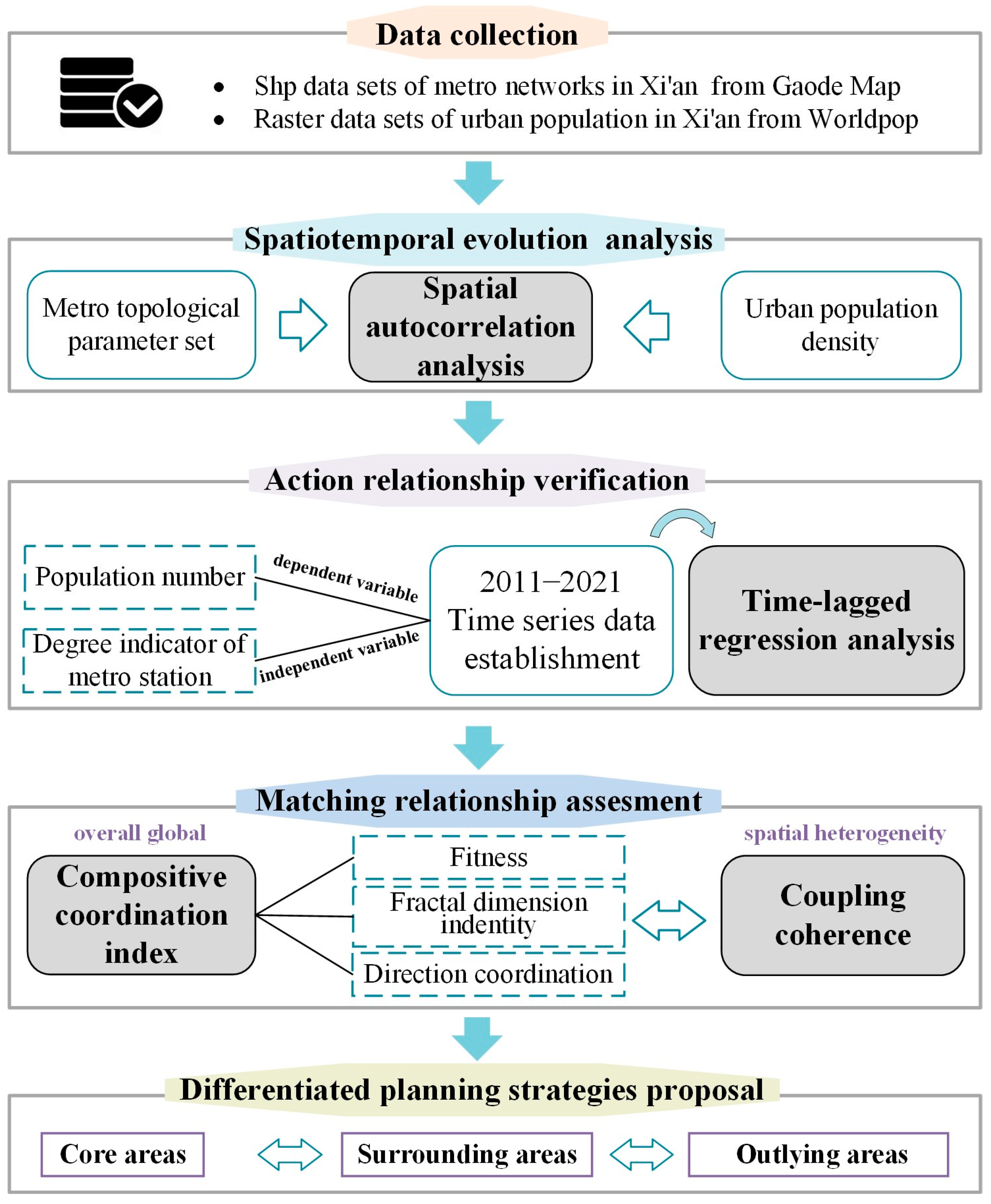
3. Materials and Methods

Based on the spatial characteristics of most metropolitan areas worldwide, most urban regions are located in the plains or shallow hilly areas [35]. As shown in the broken-line graphs of Figure 2, compared with the super-developed cities such as Shanghai and Beijing, the construction intensity of the metro networks in Xi’an City was relatively slow in middle-class areas. As a leading city in Northwest China, Xi’an is still in a period of high-speed development of metro construction and population movement in the future. Improving the rationality of spatial planning decisions is essential for cities’ high quality and intelligent growth. In addition, other cities in the middle class still face major metro construction tasks, like Zhenzhou and Suzhou cities. Moreover, the opening year of the first metro route in the above cities was around 2011, and the population size of the cities was comparable, so the metro–population interaction vein was close. Therefore, the representative city of Xi’an was selected for empirical evidence. As the six districts cover most of the metro stations, it was selected as the research scope with complete urban construction. Specifically, it includes Xincheng, Beilin, Lianhu, Yanta, Baqiao, and Weiyang districts, generally called the main urban area, with a total land area of 125 km².

In 2011, the first metro Line 2 opened in Xi’an City. At the end of 2021, the metro networks extended to 258 km. During the decade of 2011–2021, within the main urban area, the metro had grown explosively and gradually formed a network. With the implementation of regional integration policies such as the Xi’an metropolitan area, the new metro routes added in the past two years, such as Line 1 Phase 3 and Line 16, mainly serve as a cross-city connection to Xianyang City, and the spatial distribution of stations gradually moved away from Xi’an City. Therefore, this paper collects the multivariate data from 2011 to 2021: ① Metro networks (cloud platform: Gaode map). Based on the Gaode map (https://www.amap.com/(accessed on 9 February 2022)), the API interface was invocated to gradually monitor the metro spatial distribution from 2011 to 2021. ② Urban population (cloud platform: Worldpop). This study processed the permanent population density (one unit: people/km²) using the WorldPop platform (https://www.worldpop.org/ (accessed on 6 March 2022)) from 2011 to 2021, with a 100 m × 100 m grid square resolution. It is worth noting that the data accuracy was more than 95%, combined with the statistical yearbook data of various sub-district offices in Xi’an, Shaanxi Province. After obtaining the primary material, the data were preprocessed first. The ArcGIS 10.2 platform is a software product for the spatial editing of vector and raster data, with the ability to analyze and process big data in real time. With the ArcGIS 10.2 fishnet tool, the study area was divided into 1 km × 1 km square grid units, and then the population density in each grid unit was counted. At the same time, considering the distribution of metro stations and routes, a vector geographic database (GDB) was established.

Mapping metro stations and routes as nodes and links is a mainstream choice for researchers [36]. The result regarding the Space-L method is the actual spatial structure of the traffic networks, which is more suitable for studying the topological characteristics [37]. Following the determined research path plotted in Figure 1, the Space-L method was used to construct a complex topological network for the metro layout. This paper used Ucinet NetDraw to draw complex network diagrams and Matlab programming to generate an adjacency matrix. The following steps were used to model the complex rail transport networks, and the process is shown in Figure 3.

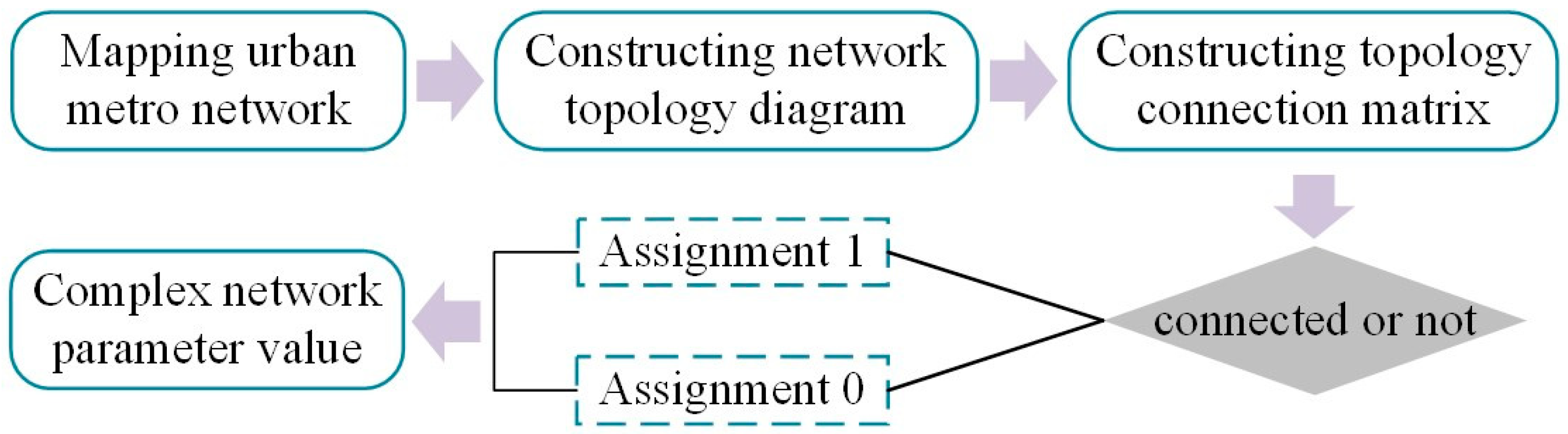
• Draw a map of the urban metro networks based on the initial metro layout and construct a topology diagram.
• Construct a topology connection matrix based on the network topology data in Space-L. If two nodes in the networks are connected, assign a corresponding value to the topological connection matrix of 1; otherwise, assign it as 0.
• Calculate the eigenvalues of Space-L networks and use the topological adjacency matrix to calculate the degree, betweenness, and closeness values.

The research content and analysis methods are listed in

Table 1. Research content and analysis methods.

Research Object	Indexes	Analysis Methods
Metro networks	Degree	Space-L complex networks
	Betweenness
	Closeness
	Moran’s I value	Spatial autocorrelation
Urban population	Permanent population density	Spatial quantization
	Moran’s I value	Spatial autocorrelation
Action relationship verification	Regression coefficient	Time-lagged regression
Spatial matching relationship	Compositive coordination index	Fitness between metro network middle and population center (W)
		$\mathrm{Fractal} \mathrm{dimension} \mathrm{identity} \mathrm{between} \mathrm{metro} \mathrm{and} \mathrm{population} (\mathfrak{R}$)
		$\mathrm{Direction} \mathrm{coordination} \mathrm{between} \mathrm{metro} \mathrm{and} \mathrm{population} (\delta$)
	Coupling coherence degree (D)	Coupling coherence

; the indexes for metro networks were obtained by the Space-L complex network model, including degree, betweenness, and closeness to measure node and link elements. The permanent population density was adopted to describe the urban population distribution using a spatial quantization model. Furthermore, this paper adopted a time-lagged regression model to verify the action relationship between the metro and urban population. Finally, the compositive coordination index and coupling coherence degree (D) were used to explore the matching relationship.

3.1. Metro Topological Parameter Set

The adjacency matrix represents the spatial relationship between each site. If there is a direct link connection between site i and site j, the value of element a_ij of matrix A is 1; otherwise, it is 0. When the adjacency matrix A = (S, L), where S is the set of stations, L is the set of route intervals, and n and m are the total numbers of stations and route intervals, respectively, then S = {s₁, s₂, …, s_n} and L = {l₁, l₂, …, l_m}.

• Degree

The degree, denoted by k_i, is the most straightforward fundamental parameter to measure the characteristics of nodes [38] and refers to the number of arcs directly connected to node i. Typically, it is mathematically defined as follows:

$$k_i={\displaystyle \frac{1}{N}}\times \sum _j{a}_{ij}$$

(1)

If a route directly connects nodes i and j, a_ij is 1; otherwise, it is 0.

In general, the degree represents the influence of a single node. The greater the node’s value, the greater its impact on the networks. The degree distribution, as the most basic topological feature, is the main basis for quantifying the metro’s size.

• Betweenness

The betweenness of node (link) i is defined as the proportion of node (link) passing through all the shortest paths in the networks, embodying the importance of the node (link) in the networks [39]. The larger the betweenness, the higher the corresponding node (link) position in the networks. This is mathematically defined as follows:

$$B_i=\sum _{k,iN,Kj}{\displaystyle \frac{D_{kj}\left(i\right)}{D_{kj}}}$$

(2)

D_kj is the number of all shortest paths connecting nodes k and j, and D_kj(i) is the number of paths through node (link) i in these shortest paths. The degree and betweenness measure the status of a single node (link) in the entire network. Compared with the degree, the betweenness depicts the potential importance of the node (link) in the networks.

• Closeness

Closeness $C_i$ is used to characterize the accessibility of nodes in spatial space, represented by the reciprocal sum of the shortest metro network distance from station i to all other stations [40]. This is mathematically defined as follows:

$$C_i={\displaystyle \frac{1}{{\sum }_{j=1}^V{d}_{ij}(i\ne j)}}$$

(3)

in which d_ij is the shortest metro network distance from station i to all other stations.

By inputting three spatial topology network diagrams from different years, the research can use a complex network analysis method to calculate the indicators of each station and each route.

3.2. Spatial Autocorrelation Model

Spatial autocorrelation analysis is used to determine whether the distribution of spatial variables is clustered, including global and local spatial autocorrelations [41,42]. The value range of Moran’s I is [−1, 1]; a value greater than 0 indicates a positive spatial correlation, and the research object has spatial aggregation. A value less than 0 shows a negative spatial correlation, and the research object has spatial discreteness. A value equal to 0 means the space is unrelated, displaying a random distribution. The spatial autocorrelation analysis was processed by GeoDa 1.20 software.

The global spatial autocorrelation index reflects the average correlation degree of a specific attribute value in the whole research area. It is generally analyzed by Moran’s I index with the following form:

$$\mathit{Globe} \mathit{Moran}’\mathit{s} \mathit{I}={\displaystyle \frac{n\sum _{i=1}^n\sum _{j=1}^n{w}_{ij}(X_i-\overline{X})(X_j-\overline{X})}{\sum _{j=1}^n\sum _{i=1}^n{w}_{ij}{(X_i-\overline{X})}^2}}$$

(4)

where n is the number of spatial units, and $\overline{X}$ is the sample mean;$X_i$and$X_j$ represent the observations of the spatial unit i and spatial unit j, respectively. w_ij is the spatial weight matrix.

In contrast to global spatial autocorrelation, the local index reflects a specific attribute value’s correlation degree and distribution pattern on a regional unit. It is generally represented by a Moran scatter plot and a decomposed Local Moran’s I index. The scatter plot is divided into four quadrants according to the mean value. H.H. (L.L.) indicates that the high-value (low-value) unit is also clustered around the high-value (low-value) unit. H.L. indicates that the high-value units are clustered around the low-value units; L.H. indicates that the low-value units are clustered around the high-value units. The formula of Local Moran’s I is as follows:

$$\mathit{Local} \mathit{Moran}’\mathit{s} \mathit{Ipq}={\displaystyle \frac{(X_i-\overline{X})\sum _{j=1}^n{w}_{ij}(X_i-\overline{X})}{\sum _{j=1}^n\sum _{i=1}^n\sum _{i=1}^n{(X_j-\overline{X})}^2}}$$

(5)

where Local Moran’s Ipq is the local spatial autocorrelation coefficient; $X_i$and$X_j$ are the observations of the spatial unit i and spatial unit j, respectively.

3.3. Time-Lagged Regression Model

In response to the research hypothesis presented in the introduction, the time-lagged model was used to demonstrate the adequacy of the research topic. With population number as the core independent variable and degree values representing the scale of metro construction as the dependent variable, this study used time series data from 2011 to 2021 for the time-lagged regression analysis [43]. Excluding the population number, the economic level also influences the size of the metro networks, while local financial revenue determines the funding for regional infrastructure development. For the hypothetical model’s simplicity and the control variables’ de-collinearity, the study adopted local financial revenue value as the control independent variable [44,45]. The calculation formula is as follows:

$$Y_t=\alpha +T{P}_{t-w}+\beta X_t$$

(6)

where Y_t denotes the integrated degree values for stations in Xi’an in year t. As the core independent variable, P presents the population number in year t; w is the lag order. T is the regression coefficient of the core independent variable. X is the control independent variable calculated by local financial revenue value, and α is the intercept term.

3.4. Compositive Coordination Index

The composite coordination index is derived from three quantitative metrics: fitness between the metro middle and the population gravity center, fractal dimension identity, and direction coordination [31].

• Fitness between metro middle and population gravity center

This paper used this method to determine the fitness degree of the metro middle and the population gravity center. The fitness represents the relative deviation between them. When w = 1, the fitness of the two is the highest; when w = 0, the fitness of the two is the worst. The formula for characterizing the fitness is as follows:

$$W=\left\{\begin{array}{c}1-{\displaystyle \frac{dom}{R}},dom\le R\\ 0,dom > R\end{array}\right.$$

(7)

where R is the equivalent radius of the city, $R=\sqrt{{\displaystyle \raisebox{1ex}{$S$}\!\left/ \!\raisebox{-1ex}{$\pi $}\right.}}$, km; S is the area of the city, km²; and dom is the spatial linear distance between the metro middle and the population gravity center, km.

• Fractal dimension identity between metro and population

As shown in Figure 4, the metro middle with the highest degree was selected as the center point for the comprehensive measurement, and the area was divided into zones with a measurement radius of 1, 2, 3, 4, 5, 10, and 15 km.

In a circular area of radius r, the relationship between metro routes’ length L(r), the area A(r) of the circular domain, and the radius r of the circle is as follows:

$$r^{1/1}\propto L_{\left(r\right)}^{1/D_L}\propto A_r^{1/2}$$

(8)

where D_L is the morphology radius dimension of metro networks, and since $r^2\propto A_{\left(r\right)}$, we obtained the following:

$$L_r=L_1{r}^{D_L}$$

(9)

After taking the logarithm of both sides, we obtained the following:

$$\ln L_r=\ln L_1+D_L\ln r$$

(10)

where L₁ is the constant coefficient, and linear regression results in D_L, which is the radius dimension of the metro network morphology.

Similarly, the urban population fractal is calculated as follows:

$$\ln S_r=\ln S_1+D_S\ln r$$

(11)

where S₁ is the constant coefficient, and linear regression results in D_S, that is, the urban population pattern radius dimension. The following equation produces the fractal dimension identity value:

$$\mathfrak{R}={\displaystyle \raisebox{1ex}{$D_L$}\!\left/ \!\raisebox{-1ex}{$D_S$}\right.}$$

(12)

When $\mathfrak{R}>1$, it is identified that the urban population density decline rate is greater than that of the metro network density, and the metro network development takes priority over the urban population. The metro networks will lead to the expansion of the urban population. When $\mathfrak{R}<1$, the metro needs to continue adapting to the urban population’s distribution. When $\mathfrak{R}=1$, the two are evolving at the same rate, which is the ideal state.

• Direction coordination between metro and population

The degree of coordination between urban metro and population distribution in azimuth includes norm and direction similarity [46]. As shown in Figure 5, taking the metro middle as the central point, the area was divided into eight fan-shaped regions according to the orientation.

The population number of the i_th fan-shaped area is p_i, and the length of the track line is l_i. The following vector can then express the population distribution in the orientation:

$$\underset{p}{\to }\left({\displaystyle \frac{p_1}{p}},{\displaystyle \frac{p_2}{p}},\dots {\displaystyle \frac{p_n}{p}}\right)=(x_1,x_2,\dots ,x_n)$$

(13)

where $\underset{p}{\to }$ represents the distribution vector of the population in the direction; p_i represents the population of the i_th sector, ten thousand people; p represents the total population, ten thousand people; and x_i represents the population proportion of the i_th sector, $\sum _{i=1}^n{x}_i=1$.

The following vectors can represent the orientation distribution of the urban metro networks:

$$\underset{l}{\to }\left({\displaystyle \frac{l_1}{l}},{\displaystyle \frac{l_2}{l}},\dots {\displaystyle \frac{l_n}{l}}\right)=(y_1,y_2,\dots ,y_n)$$

(14)

where $\underset{l}{\to }$ represents the distribution vector of the metro networks in the direction; l_i represents the length of the metro route in the i_th sector area, km; l represents the total length of the metro networks in the main urban area, km; and y_i represents the proportion of the length of the metro networks in the i-sector area, $\sum _{i=1}^n{y}_i=1$.

The norm similarity calculation formula is as follows:

$$\phi =\left\{\begin{array}{c}1-{\displaystyle \frac{‖\underset{L}{\to }‖-‖\underset{P}{\to }‖}{‖\underset{P}{\to }‖}},‖\underset{L}{\to }‖\le 2‖\underset{P}{\to }‖\\ 0,‖\underset{L}{\to }‖>2‖\underset{P}{\to }‖\end{array}\right.$$

(15)

The direction similarity calculation formula is as follows:

$$\sigma =\left\{\begin{array}{c}1-{\displaystyle \frac{2}{\pi }}\times \theta ,0\le \theta \le {\displaystyle \frac{\pi }{2}}\\ 0,{\displaystyle \frac{\pi }{2}}<\theta \le \pi \end{array}\right.$$

(16)

of which, θ is the angle between two vectors.

The formula for calculating the direction coordination degree is δ = φ $\times$ σ. The closer δ is to 1, the better the coordination is.

3.5. Coupling Coherence Model

Based on the population number and metro station indicators of each 1 km × 1 km square grid unit, the coupling coherence model [32] was used to measure the spatial and temporal differentiation characteristics of the matching relationship. The calculation formula is as follows:

$$C=2\sqrt{{\displaystyle \raisebox{1ex}{$(E_i\times S_i)$}\!\left/ \!\raisebox{-1ex}{${(E_i+S_i)}^2$}\right.}}$$

(17)

$$T=\alpha \times E_i+\beta \times S_i$$

(18)

$$D=\sqrt{C\times T}$$

(19)

where E_i and S_i are the standardized value of the population number and the integrated value of the metro station at the i_th grid unit; C is the degree of coupling; and T is the integrated evaluation index of the population and the metro. D is the degree of coupling coherence, reflecting the level of coupling and coordination between the population and the metro; the value of D is 0~1. The higher the value is, the higher the degree of coupling coherence between the two sub-systems is.

4. Results

4.1. Spatiotemporal Evolution of Metro Networks and Urban Population

The sites were numbered, and the adjacency matrixes were built based on whether the sites were directly connected. This study simplified the metro stations and routes as Space-L networks from 2011 to 2021 and took topology networks as plotted in Figure 6 as the example in three time slices of 2011, 2016, and 2021. Consequently, the complex network characteristics of the Xi’an metro were depicted using the parameters of degree, betweenness, and closeness using Matlab R2021b software.

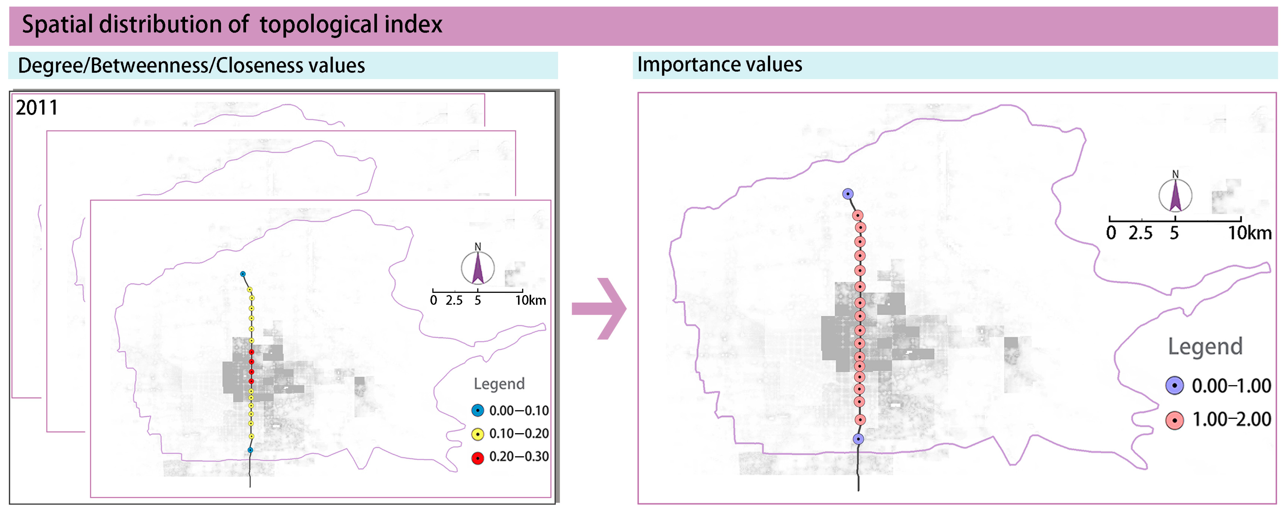
4.1.1. Metro Topology Networks

The metro network model calculated the count number of station degree values for the six time nodes of metro construction in Xi’an from 2011 to 2021 (Figure 7). In 2011, Xi’an’s first metro Line 2 opened, and there were no transfer stations. The degree values were between 1 and 2, and the proportions of stations with values ranging from 1 to 2 were 11.11% and 88.89%, respectively. Until the opening of Line 1 in 2013, the transfer hub was formed at the Bei Da Jie station, and the degree value at the station appeared as 5. After that, the proportion of transfer stations with high degrees (values of 4 and 5) increased exponentially, reaching 10.53% in 2021, showing the further complexity of the networks. By comparing the six topological models, it was found that the proportion distribution of the degree values at 2 in all phases reached the maximum, which indicates that the number of stations that were connected to only two neighboring stations was the highest in the rail networks, with a proportion of more than 75%.

Figure 8 illustrates the spatiotemporal evolution characteristics of metro network metrics. The betweenness and closeness of stations with high degree values were also great, mainly showing that the three indicators have a positive correlation. It is worth noting that the degree value focuses more on the accessibility to other stations and less on the spatial location weight of the station than the betweenness and closeness. Some nodes with high degrees were located at transfer stations in the city’s outlying areas, such as Bei Ke Zhan, Xing Zheng Zhong Xin, and Shuang Zhai. On the contrary, the sites with high values of betweenness and closeness were mainly concentrated in the inner circle with a noticeable spatial spillover effect. The mobility rate between the transfer and other stations is obviously frequent [47,48]. For instance, Bei Da Jie, Tong Hua Men, and Xiao Zhai stations had higher values than others. Subsequently, Yaahp V2.10 software for the AHP analysis method was employed to assign weighting values to indexes and obtain a comprehensive indicator characterized by importance. The transfer nodes such as Bei Da Jie, An Yuan Men, and Wu Lu Kou have greater connectivity with other links, so the importance was high. Among them, Bei Da Jie station as the metro middle ranked first, with values of 1.21, 2.29, and 2.28, respectively. The clustering, interoperability, and connectivity of these stations may attract the traveling population quickly and efficiently increase the supply of rail transport, which can cause the aggregation of demographic elements in the stations’ surrounding areas [49].

This study interrupted and separated metro routes according to the location of station distribution, described the status of link elements using betweenness in complex topological networks, and performed spatial visualization analysis. The evolutionary characteristics of the betweenness value of links from 2011 to 2021 are shown in Figure 9. The larger the value, the higher the position of the corresponding link in the networks. The betweenness index of metro links had a decreasing circular distribution from the center to the periphery, with values ranging from 0 to 0.3, with an apparent spatial spillover effect.

The spatially dependent features of metro links were further explored using the ArcGIS 10.2 tool. The global Moran’s I value reduced from 0.782 in 2011 to 0.510 in 2021. The p-scores were less than 0.01, and the z-scores were more than 2. The high-confidence results indicate a significant spatial autocorrelation of metro routes with a spatial spillover effect. In the process of metro construction, the Moran index of metro routes shows a spiral rather than a straight-line decline (

Table 2. Moran’s I value for metro routes.

Year	2011	2012	2013	2014	2015	2016	2017	2018	2019	2020	2021
Value	0.782 ***	0.782 ***	0.459 ***	0.459 ***	0.459 ***	0.800 ***	0.800 ***	0.391 ***	0.274 ***	0.510 ***	0.510 ***

*** Passed the significance test at the 1 percent level.

); this may be because the spatial dependence of metro routes was characterized by agglomeration–homogenization–agglomeration with the opening of new routes. Ultimately, the general trend was gradually weaker, possibly due to the metro element’s homogenization distribution with the topology network densification [50].

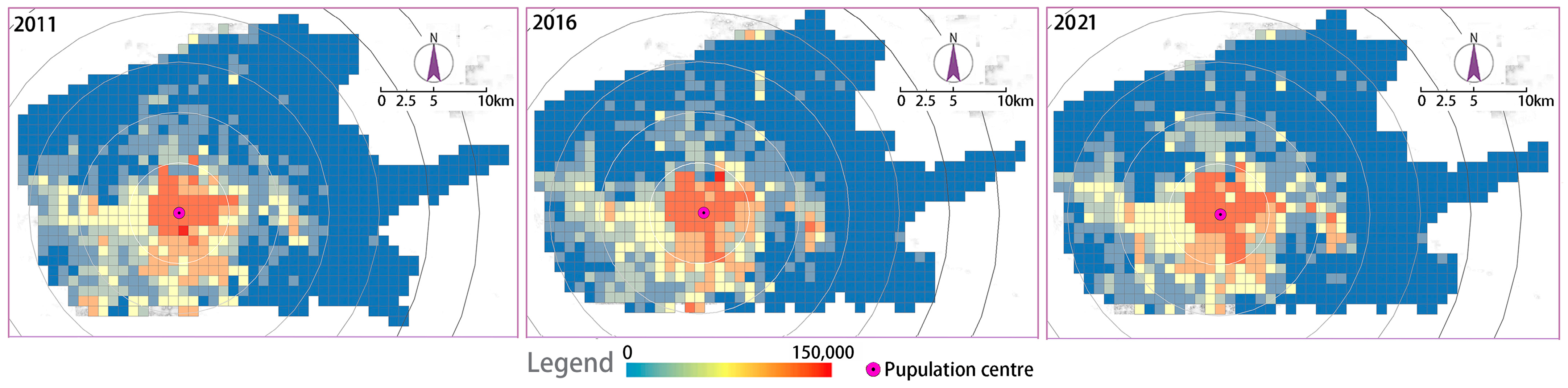
4.1.2. Urban Population

Meanwhile, from 2011 to 2021, the permanent population density data were intercepted in this study, and then, a 1 km × 1 km grid network was applied as the research unit. Furthermore, the average center tool of ArcGIS 10.2 was utilized to identify the population center year by year. The population density was plotted in Figure 10, in which a circle-type spatial distribution pattern at the core edge existed in the main urban area of Xi’an. The study divided the circle layer gradually according to the interval of 10 km [51]; notably, the high-density areas were located in the 0–10 km circle layer, where the population density of the peripheral circle layer was more than 8000 people/km². From 2011 to 2021, the population density of each unit changed. Nevertheless, the circle pattern remained stable and invariant. It is worth noting that the average population density shows an increasing trend with 5162.53, 5470.76, and 5718.49 persons/km², which indicates that the population size of Xi’an has continued to increase under the background of rapid urbanization in the past decade.

With the spatial autocorrelation model analysis, the global Moran’s I values of the population density in the main urban area of Xi’an were greater than 0, indicating that the population distribution shows a significant positive spatial dependence. The Moran indexes ranging from 0.737 to 0.759 show a smooth trend, and the population distribution was consistently clustered over a decade (

Table 3. Moran’s I value for urban population.

Year	2011	2012	2013	2014	2015	2016	2017	2018	2019	2020	2021
Value	0.759 ***	0.737 ***	0.741 ***	0.745 ***	0.741 ***	0.742 ***	0.740 ***	0.742 ***	0.742 ***	0.742 ***	0.742 ***

*** Passed the significance test at the 1 percent level.

). In particular, the concentration of infrastructural resources has exerted thrust on population distribution to keep growing [52,53,54]. In the future, the population spatial distribution may still be in a state of aggregation, unlike the weaker spatial dependence of metro elements. As the complexity of the metro topological network increased, its spatial dependence was less than the population distribution, gradually leading to a centrifugal expansion of the urban population.

The Local Moran index was employed to detect the range and location of outliers or clusters [55]. The LISA maps displayed in Figure 11 (p < 0.05) roughly reflect the spatial aggregation heterogeneity of population density inside each grid. It can be observed that the population was mainly concentrated in the 0–10 km circle layer (high–high aggregation), while the LL aggregation (low–low aggregation) was in the urban fringe areas. This result may be due to the siphoning effect of metro and other infrastructure resources on population attraction, showing the spatial heterogeneity of unbalanced resource distribution.

4.2. Action Relationship Verification

There may be a lag effect in the interaction between the metro networks and the urban population during the evolution of the city. This study fitted time-lagged regressions of metro networks and urban population for the period of 2011–2021, revealing the action relationship over ten years. As illustrated in

Table 4. Lagged effects of metro networks and population distribution.

Variable	Current Period	Lag Order 1	2	3
Population	0.614 **	1.301 **	1.508 **	0.802
	(5.40)	(6.76)	(3.85)	(0.68)
LFR	107.570 *	100.600	104.982	−253.900
	(2.44)	(1.86)	(0.79)	(0.81)
Constant	−1695.39	−1856.75	−1983.13	3543.74
	(2.67)	(2.35)	(0.98)	(0.72)
R-squared	0.82	0.87	0.74	0.53

* p < 0.05; ** p < 0.01.

, the regression coefficients for station index lagged orders 0–2 were significantly positive with p < 0.01. This indicates that the population number had an obvious functional relationship with the construction of the metro networks. This relationship was highlighted in the next 1–2 years with a positive feedback effect, and the regression coefficient increased from 1.301 to 1.508. The aggregation of the population gradually triggered travel demand, which attracted the growth of transport facilities. The regression results show that the metro and population were positive mechanisms in the urban development process, which also verified the research hypothesis presented in the introduction chapter. That is, a specific interrelationship existed between urban metro and population distribution.

4.3. Spatiotemporal Evolution of Matching Relationship

On the basis of clarifying the evolution characteristics of the metro networks and population distribution, this study applied the compositive coordination index to assess the overall matching degree of the two. Then, the coupling coherence model was used to identify the spatial heterogeneity.

4.3.1. Global Matching Relationship

• Fitness between metro middle and population gravity center

From 2011 to 2021, the coordinates of the population center were (108.950, 34.265), (108.955, 34.265), and (108.952, 34.264). Since the spatial distance between the metro middle and the population gravity center was low, the fitness values were 0.937, 0.914, and 0.927 (

Table 5. Fitness between metro network middle and population gravity center.

Year	Coordinates of the Population Center	Distance (km)	Fitness Values
2011	(108.950, 34.265)	1.02	0.937
2016	(108.955, 34.265)	1.40	0.914
2021	(108.952, 34.264)	1.18	0.927

), with a high matching level. In the early stages, metro planning was highly catered to the population distribution, and the fitness value was at its highest level in 2011. With the increase in new routes, the metro middle deviated from the population gravity center, which signals a shift in the interaction of the metro networks’ influence on the population.

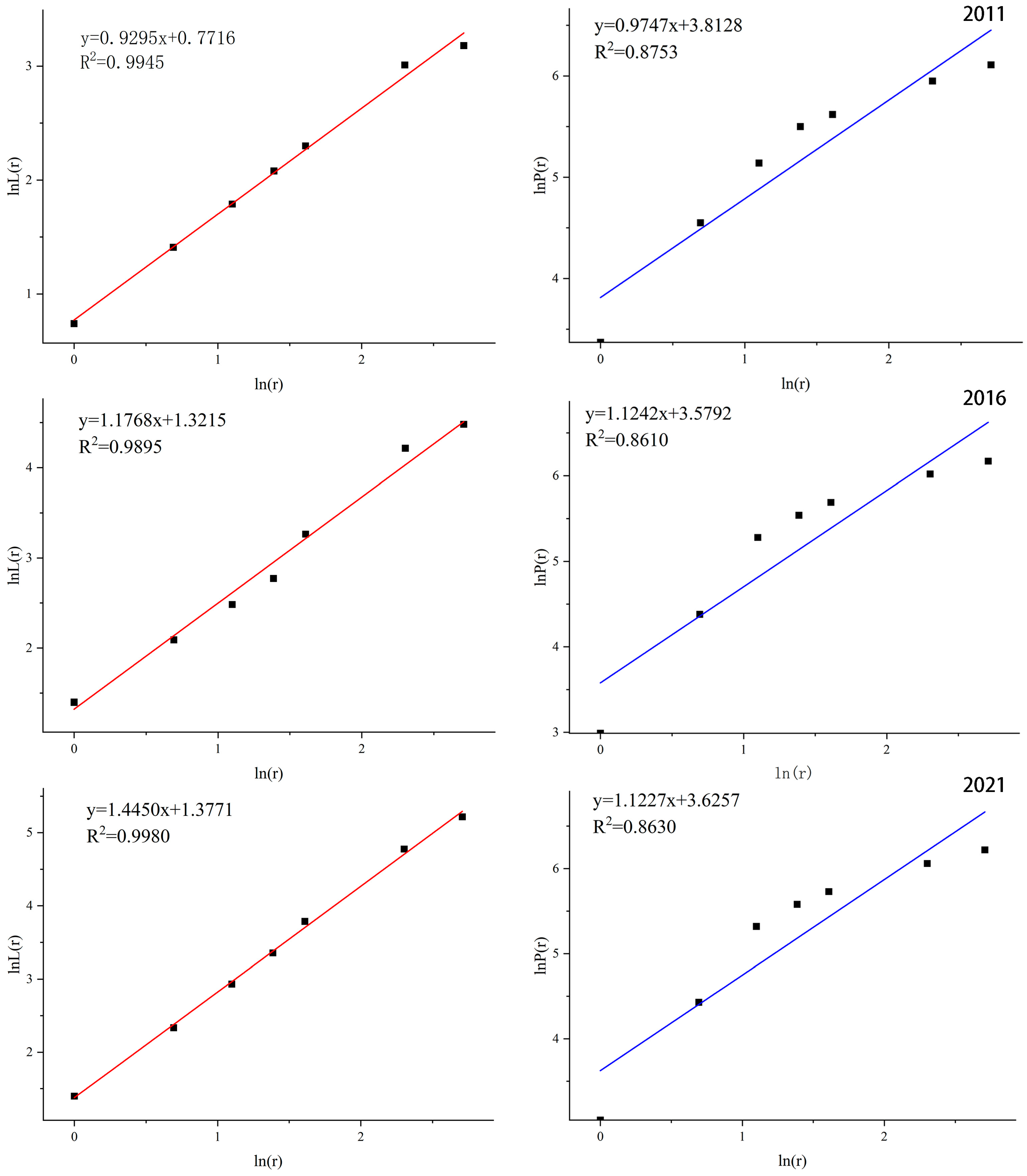
• Fractal dimension identity between metro and population

By calculating and taking the logarithm of the metro network length and population number in different radius rings, the paper regressed the above data linearly, as shown in Figure 12. In 2011, 2016, and 2021, the fractal dimension D_L of metro networks were 0.93, 1.18, and 1.45, respectively, and the D_S values of population density were 0.97, 1.24, and 1.22, respectively. The fractal dimension values were all less than 2, which proved that the density of metro networks and urban population gradually decreased from the center outward. The fractal identity $\mathfrak{R}$ were 0.96, 0.95, and 1.19 from 2011 to 2021, respectively, indicating that the metro development in the surrounding areas of Xi’an City was still lagging behind the urban population layout until 2016, which passively adapted to the population distribution. And in 2021, the fractal identity $\mathfrak{R}$ reached 1.19, exceeding 1, proving that the decline rate of metro network density was less than that of urban population density, and the development of the metro networks actively guided the expansion of the urban population. This result can further corroborate the results of spatial autocorrelation in Section 4.1.

• Direction coordination between metro and population

This paper calculated the statistical results in each zone involving the following two aspects: the length of metro routes (one unit: km) and the number of permanent population (one unit: 10,000 people). Subsequently, combined with Equations (13) and (14), the distribution vectors in 2011, 2016, and 2021 were obtained in

Table 6. Distribution vectors.

Time	Permanent Population	Metro Networks
2011	$\underset{p}{\to }=(0.12, 0.06, 0.10, 0.09, 0.13, 0.20, 0.19, 0.11)$	$\underset{l}{\to }=(0.00, 0.28, 0.28, 0.00, 0.00, 0.22, 0.22, 0.00)$
2016	$\underset{p}{\to }=(0.13, 0.09, 0.10, 0.09, 0.12, 0.18, 0.17, 0.12)$	$\underset{l}{\to }=(0.19, 0.09, 0.07, 0.09, 0.14, 0.10, 0.10, 0.23)$
2021	$\underset{p}{\to }=(0.10, 0.09, 0.10, 0.10, 0.12, 0.18, 0.18, 0.12)$	$\underset{l}{\to }=(0.15, 0.13, 0.06, 0.06, 0.13, 0.15, 0.18, 0.14)$

. The direction coordination degree values were 0.32, 0.67, and 0.82, respectively.

The comprehensive coordination index was computed by multiplying the above three indicators. From the perspective of Xi’an as a whole, the matching values between the metro networks and the population increased from 0.29 to 0.90, with a growth rate of 210.34%. As the metro networks were built in Xi’an City, the relationship between the demand and supply of the metro was gradually being balanced.

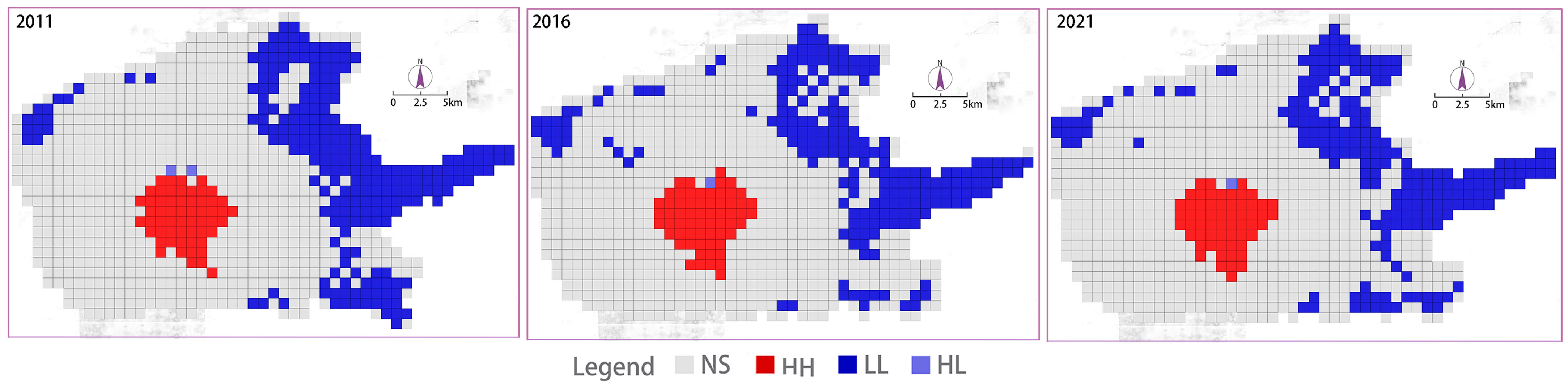
4.3.2. Spatial Heterogeneity of Matching Relationship

The comprehensive coordination index assessed the relationship between metro networks and urban population matching from a global perspective, and it may blur the spatial heterogeneity of the coordination relationship. As presented in Figure 13, the coupling coherence degree attached to grid cells can supplement the gap through Equations (17)–(19). According to existing studies [32], three ranks of matching relationships were classified according to the D value: D ≤ 0.25 is a low-level mismatch; 0.25 < D ≤ 0.5 is a medium-level fit; and 0.5 < D is high-level overdevelopment. From 2011 to 2021, the matching value at most spatial units improved from low-level mismatch (D ≤ 0.25) to medium-level fit (0.25 < D ≤ 0.5), and there was apparent spatial heterogeneity (Figure 13). Among them, the proportion of spatial units with a low-level mismatch decreased from 95.66% to 82.85%. Correspondingly, the proportions of spatial units with high-level overdevelopment (0.5 < D) were 3.11%, 8.19%, and 13.05% from 2011 to 2021, respectively. Overall, the spatial units that improved from a low to medium level were mainly clustered in the areas along the metro routes. The opening of stations and routes could boost the accessibility of the areas around the metro networks, which could meet the daily travel demands of residents. It is worth noting that the spatial units with a high-level matching (0.5 < D) between population distribution and the metro networks have always been mainly concentrated in the core circle of 0–10 km, where there were more hub metro stations, which significantly improves the efficiency of the metro supply to meet the demand of high-density population traveling.

Overall, the spatial heterogeneity of the matching relationship between metro networks and urban populations in Xi’an City gradually narrowed in the core, surrounding, and outlying areas. Specifically, the 0–10 km core areas have always served as a cluster of high-quality resources and attracted the layout of metro facilities. The matching relationship has always been at a high level compared to other regions. The average coupling value increased from 0.26 to 0.41 from 2011 to 2021, and the proportion of grid units with a medium-level fit rose from 21.51% to 55.65%. However, it faces tremendous pressure on the supply side of traveling services. In 10–20 km surrounding areas, the proportion of units with a medium-level fit increased from 2.58% in 2011 to 22.99% in 2021. It is worth noting that the average coupling coherence degree rose from 0.16 to 0.20. The highest proportion of spatial units with a low-level mismatch in the outlying areas still existed (88.30% in 2021). Regarding average values, the coupling coherence degree value has gradually increased from 0.13 to 0.15, with a slower growth rate.

5. Discussion

At present, many cities are still facing the construction of the metro networks. The spatial relationship between the metro networks and the population should be clarified, which determines the utilization efficiency of the infrastructure resources. On the one hand, the development of rail transit systems is an essential driver of the evolution of urban demographics. To some extent, urban public transport may change the land use value and accessibility along the routes and around the stations [56]. These changes cause land development and thus promote the evolution of urban population distribution.

On the other hand, urban population, as a typical element of spatial structure, its development scale, zoning layout, and density produces the passenger flow aggregation, which determines travel demand [19]. The matching relationship between metro networks and urban population impacts the metro networks’ utilization efficiency. At the same time, the bidirectional mechanism mentioned above always runs through the whole urban development process. As plotted in Figure 14, in the early stage of metro development, the urban population is the root cause of traffic demand, and the metro skeleton needs to adapt to travel demand, showing the characteristics of “passive adaptation” [7]. Afterward, the metro networks offer the “active guidance” mode, which can lead the population to spread to the outlying areas.

According to the results of Moran’s I index and fractal dimension identity, the population in Xi’an City has continued to be in an agglomeration state until 2021. On the contrary, the distribution of metro elements shows a centrifugal diffusion, which proves that the metro network construction has reached a mature networked stage. The role of the metro in Xi’an City has crossed from passive adaptation to active guidance in the urban population. Through the spatiotemporal evolution analysis of the coupling coherence model, although the comprehensive coordination index of the metro networks and urban population increased from 2011 to 2021, the matching relationship between the two shows a significant heterogeneity in space. Therefore, differentiated spatial planning strategies were proposed. The core areas with the highest population density face the greatest pressure to provide metro facilities. In this area, it is recommended that land with TOD be developed as a guide, significantly improving the accessibility of metro facilities and forming a composite and efficient land development mode. In the surrounding areas, the dual elements regarding the metro and population layout should be planned comprehensively. The land layout should be reasonably guided to converge along the metro routes, and the metro resources should be targeted for the units with higher population density. Based on the phenomenon of imbalance between supply and demand, planning strategies in outlying areas should focus on improving the efficiency of connecting the metro with other types of public transport, reducing the time distance between residents and metro stations. As explained in Section 3, the differentiated planning strategies can be extended to similar cities with the same realities as Xi’an, such as Zhengzhou et al. In some cities where the urban development of metro construction and population movement is still at a high speed, these measures can be targeted to ameliorate the wastage of resources due to the spread of the metro facilities.

6. Conclusions

The matching relationship between a city’s metro and its population is essentially one of supply and demand, which profoundly impacts the efficiency of rail transport utilization. This study’s content advanced upon previous research that only selected a single time node and global space unit for static analysis [4,9] and emphasized the spatiotemporal evolution analysis in units of the grid.

Following the complex topology networks adopted by Jiang et al. and Sienkiewicz et al. [26,27], the metro networks were explored from node and link elements, and the characteristics were measured using degree, betweenness, and closeness. Meanwhile, the spatial autocorrelation model analyzed the spatial evolution of the metro networks and population density from 2011 to 2021 [7]. In this paper, we also argued the specific significant relationship between metro and population to respond to the research hypothesis as a process of a closed-loop study. Then, this paper used the compositive coordination index and coupling coherence degree to assess the matching relationship variation from global and local scales. From the results of the above empirical analyses, the research conclusions were summarized, and the application of the findings to planning practice was facilitated, i.e., the fourth conclusion.

• The network distribution had a trend of centrifugal dispersion with Moran’s I values from 0.78 in 2011 to 0.51 in 2021, respectively. The population distribution remained highly spatially dependent with Moran’s I values greater than 0.7. There existed a specific positive time-lagged interrelationship between urban metro and population distribution in the process of urban development due to the regression coefficient being more than 0.
• Along with the increased complexity of the metro topology networks, the compositive coordination index between the metro networks and the population increased from 0.29 to 0.90. The fractal identity $\mathfrak{R}$ was 1.19 until 2021, indicating that the role of the metro networks gradually crossed from “passive adaptation” to “active guidance”.
• From 2011 to 2021, there was obvious spatial heterogeneity for matching relationships. The coupling coherence degree in the core areas increased from 0.26 in 2011 to 0.41 in 2021, while the value of the outlying areas was only 0.15 until 2021.
• In the future planning policy-making of Xi’an, differentiated spatial planning strategies were proposed for core, surrounding, and outlying areas. The planning program should abandon the sprawl expansion of metro construction.

The coordinated development of urban metro networks and population distribution involves multiple levels and disciplines. This study emphasized the spatial and temporal matching heterogeneity of the metro and population element, and the analysis adopted big data such as population density with desensitization, ignoring the travel data carried by individual residents. In addition, in the process of urban development, building environment elements instead of urban population also balances the metro network distribution. More building spatial variables, such as land use function, density, urban form, etc., should be selected to fully explore the intrinsic operational relationship between rail transport and urban spatial structure.

References

- Manouvrier-Hanu, S.; Walbaum, R.; Gayot, C. Progress of construction of the rapid transit tunnel. Aquaculture 1998, 160, 283–303. [Google Scholar] [CrossRef]
- Li, Z.; Xia, T.; Xia, Z.; Wang, X. The impact of urban rail transit on industrial agglomeration based on the intermediary effects of factor agglomeration. Math. Probl. Eng. 2021, 2021, 6664215. [Google Scholar] [CrossRef]
- Li, W.; Yang, D. Spatial analysis logic for urban transportation based on the “shaped by flow” concept. City Traffic 2020, 18, 1–8. [Google Scholar] [CrossRef]
- Hao, S.Y.; Yan, J.W.; Teng, S.H. Rail transit construction and optimization of urban spatial structure: Experience and enlightenment from Taipei. City Plan. Rev. 2013, 37, 62–66. [Google Scholar]
- Shu, H.Q.; Shi, X.F. The effect of Tokyo metropolis circle’s railway system to urban spatial structure development. Urban Plan. Int. 2008, 23, 105–109. [Google Scholar] [CrossRef]
- Calvo, F.; Eboli, L.; Forciniti, C.; Mazzulla, G. Factors influencing trip generation on metro system in Madrid (Spain). Transp. Res. Part D-Transp. Environ. 2019, 67, 156–172. [Google Scholar] [CrossRef]
- Wang, Z.; Li, S.; Song, J. Analysis of transfer service level between rail and ground bus based on bivariate spatial autocorrelation: Taking the morning peak in Beijing as an example. J. Hunan City Univ. 2023, 32, 44–49. [Google Scholar] [CrossRef]
- Cipriani, E.; Gori, S.; Petrelli, M. Transit network design: A procedure and an application to a large urban area. Transp. Res. Part C Emerg. Technol. 2012, 20, 3–14. [Google Scholar] [CrossRef]
- Cheng, X.; Zhang, X.; Shi, C.; Liu, Y.; Ding, L. Coupling effects analysis of jobs-housing distribution and rail transit network. J. Harbin Inst. Technol. 2022, 54, 35–43. [Google Scholar] [CrossRef]
- Seaton, K.A.; Hackett, L.M. Stations, trains and small-world networks. Phys. A Stat. Mech. Its Appl. 2004, 339, 635–644. [Google Scholar] [CrossRef]
- Zhang, J.; Wang, S.; Wang, X. Comparison analysis on vulnerability of metro networks based on complex network. Phys. A Stat. Mech. Its Appl. 2018, 496, 72–78. [Google Scholar] [CrossRef]
- Li, Y. Application of Bayesian hierarchical spatiotemporal model in inter-provincial population inflow analysis. Stat. Decis. Mak. 2018, 34, 73–77. [Google Scholar] [CrossRef]
- Deville, P.; Linard, C.; Martin, S.; Gilbert, M.; Stevens, F.R.; Gaughan, A.E.; Blondel, V.D.; Tatem, A.J. Dynamic population mapping using mobile phone data. Proc. Natl. Acad. Sci. USA 2014, 111, 15888–15893. [Google Scholar] [CrossRef] [PubMed]
- Kaza, N.; Nesse, K. Characterizing the regional structure in the United States: A county-based analysis of labor market centrality. Int. Reg. Sci. Rev. 2021, 44, 560–581. [Google Scholar] [CrossRef]
- Yu, Y.; Ren, H.; Gao, X. New features of the spatial pattern evolution of China’s urban population-analysis based on 2000–2020 census data. Popul. Econ. 2022, 43, 65–79. [Google Scholar]
- Chen, T.; Pan, H. Coupling Metro network with household and employment pattern: A case study of Shanghai. J. Urban Plan. 2020, 64, 32–38. [Google Scholar] [CrossRef]
- Deng, Y.; Cai, J.; Yang, Z.; Wang, H. Analysis of traffic time reachability measurements and spatial characteristics in Beijing urban area. Acta Geogr. Sin. 2012, 6, 169–178. [Google Scholar]
- Feng, H.; Li, C.; Zhang, S. Study on coordinated development of urban spatial arrangement and trail traffic based on GIS. J. Northwest Univ. 2014, 44, 821–824. [Google Scholar] [CrossRef]
- Chen, J.; Chen, X. The research of the spatial structure network of urban agglomeration based on the development of network spatial: A case study of Guanzhong urban agglomeration. Mod. Urban Stud. 2022, 37, 111–118. [Google Scholar] [CrossRef]
- Chen, B. Rail Transit Development of the Pearl River Delta planning, obstacles and history. Urban Rail Transit 2018, 4, 13–22. [Google Scholar] [CrossRef]
- Li, Y.; Monzur, T. The spatial structure of employment in the metropolitan region of Tokyo: A scale-view. Urban Geogr. 2018, 39, 236–262. [Google Scholar] [CrossRef]
- Szeto, W.Y.; Jiang, Y.; Wong, K.I.; Solayappan, M. Reliability-based stochastic transit assignment with capacity constraints: Formulation and solution method. Transp. Res. Part C-Emerg. Technol. 2013, 35, 286–304. [Google Scholar] [CrossRef]
- Wang, C.; Hokao, K. The evolution of population distribution in metro city: A case of Fukuoka city, Japan. Sci. Geogr. Sin. 2010, 30, 516–520. [Google Scholar] [CrossRef]
- Bothe, K.; Hansen, H.K.; Winther, L. Spatial restructuring and uneven intra-urban employment growth in metro- and non-metro-served areas in Copenhagen. J. Transp. Geogr. 2018, 70, 21–30. [Google Scholar] [CrossRef]
- Irsal, R.M.; Hasibuan, H.S.; Azwar, S.A. Spatial modeling for residential optimization in dukuh atas Transit-Oriented Development (TOD) area, Jakarta, Indonesia. Sustainability 2023, 15, 530. [Google Scholar] [CrossRef]
- Jiang, B. A topological pattern of urban street networks: Universality and peculiarity. Phys. A Stat. Mech. Its Appl. 2007, 384, 647–655. [Google Scholar] [CrossRef]
- Sienkiewicz, J.; Hołyst, J.A. Statistical analysis of 22 public transport networks in Poland. Phys. Rev. E 2005, 72, 046127. [Google Scholar] [CrossRef] [PubMed]
- Du, P.; Hou, X. Spatial simulation of population in China’s coastal zone based on multi-source data. J. Geo-Inf. Sci. 2020, 22, 207–217. [Google Scholar] [CrossRef]
- Hou, Q.H.; Xing, Y.T.; Wang, D.; Liu, J.C.; Fan, X.Y.; Duan, Y.Q. Study on coupling degree of rail transit capacity and land use based on multivariate data from cloud platform. J. Cloud Comput.-Adv. Syst. Appl. 2020, 9, 4. [Google Scholar] [CrossRef]
- Wu, Z.; Ye, Z. Research on urban spatial structure based on Baidu heat map: A case study on the central city of Shanghai. Urban Plan. 2016, 40, 33–40. [Google Scholar] [CrossRef]
- Wang, Y.P.; Chen, K.M.; Ma, C.Q. Quantitative analysis of coordination between rail transit network configuration and urban form. J. Railw. Eng. Soc. 2008, 11, 11–15. [Google Scholar] [CrossRef]
- Ji, Y.; Jiang, H.M. Spatial and temporal differences and influencing factors of the adaptation degree of aging and pension resources in the new era. Sci. Geogr. Sin. 2022, 42, 851–862. [Google Scholar] [CrossRef]
- Shi, D.H.; Fu, M.C. How does rail transit affect the spatial differentiation of urban residential prices? A case study of Beijing subway. Land 2022, 11, 1729. [Google Scholar] [CrossRef]
- Liu, J.M.; Hou, X.H.; Xia, C.Y.; Kang, X.; Zhou, Y.J. Examining the spatial coordination between metrorail accessibility and urban spatial form in the context of big data. Land 2021, 10, 580. [Google Scholar] [CrossRef]
- Mu, G.; Tan, S. Studies of urban geomorphology and the urban landforms in plain region. J. Southwest Teach. Univ. 1990, 34, 470–477. [Google Scholar] [CrossRef]
- Zhang, L.; Zhu, M.; Yang, W.C.; Dong, D. Modeling and analysis of network topological characteristics of urban rail transit. Urban Mass Transit 2015, 18, 28–31. [Google Scholar] [CrossRef]
- Meng, Y.; Tian, X.; Li, Z.; Zhou, W.; Zhou, Z.; Zhong, M. Comparison analysis on complex topological network models of urban rail transit: A case study of Shenzhen Metro in China. Phys. A 2020, 559, 125031. [Google Scholar] [CrossRef]
- Pang, L.; Ren, L.J.; Yun, Y.X. Research on interactive development of rail transit and spatial structure of London metropolitan circle from the perspective of complex system. J. Hum. Settl. West China 2022, 37, 98–105. [Google Scholar] [CrossRef]
- Li, C.; Ma, R.; Wang, Y.; Wang, Z. Characteristics and structure analysis of urban slow mode traffic network. J. Traffic Transp. Eng. 2011, 11, 72–78. [Google Scholar] [CrossRef]
- Zhan, X.; Lin, A.W.; Sun, C. Centrality of public transportation network and its coupling with bank branches distribution in Wuhan City. Prog. Geogr. 2016, 35, 1155–1166. [Google Scholar] [CrossRef]
- Kumari, M.; Sarma, K.; Sharma, R. Using Moran’s I and GIS to study the spatial pattern of land surface temperature in relation to land use/cover around a thermal power plant in Singrauli district, Madhya Pradesh, India. Remote Sens. Appl. Soc. Environ. 2019, 15, 100239. [Google Scholar] [CrossRef]
- Wang, Y.Q.; Shao, M.A. Spatial variability of soil physical properties in a region of the loess plateau of pr China subject to wind and water erosion. Land Degrad. Dev. 2013, 24, 296–304. [Google Scholar] [CrossRef]
- Zhang, R.Z. Study on the factors affecting the land price of Beijing, Tianjin and Hebei based on the multivariate cointegration lag regression model. J. Cent. China Norm. Univ. (Nat. Sci.) 2017, 51, 607–614. [Google Scholar] [CrossRef]
- Becker, T.E. Potential problems in the statistical control of variables in organizational research: A qualitative analysis with recommendations. Organ. Res. Methods 2005, 8, 274–289. [Google Scholar] [CrossRef]
- York, R. Control variables and causal inference: A question of balance. Int. J. Soc. Res. Methodol. 2018, 21, 675–684. [Google Scholar] [CrossRef]
- Chen, K.; Fan, D.; Ma, C. Calculation of urban rail transit network scale based on passenger distributing centers. J. Chang. Univ. 2009, 29, 78–81. [Google Scholar] [CrossRef]
- Guo, Q.; Wu, D.; Bao, J. Evaluation of accessibility in urban rail transit network of Beijing based on transfer efficiency index and the analyze of its cause. Econ. Geogr. 2012, 32, 38–44. [Google Scholar] [CrossRef]
- Chen, S.P. Urban rail transit network accessibility metrics and spatial characteristics analysis—Guangzhou city as an example. Geogr. Geo-Inf. Sci. 2013, 2, 113–117. [Google Scholar]
- Cao, Z. Configuration of urban commercial centers and transport centers: Evidence from Tokyo transit network and urban morphology based on the complex network analysis. Int. Urban Plan. 2020, 35, 42–53. [Google Scholar] [CrossRef]
- Cui, X.; Yu, B.; Liang, P.; Wang, L.; Zhang, L. Urban rail transit station type identification and job-housing spatial rebalancing based on passenger flow and land use: Taking Chengdu as an example. Mod. Urban Res. 2021, 36, 68–79. [Google Scholar] [CrossRef]
- Niu, J.; Du, H. Coordinated development evaluation of population-land-industry in counties of western China: A case study of Shaanxi province. Sustainability 2021, 13, 1983. [Google Scholar] [CrossRef]
- Li, X.; Lu, Z.; Hou, Y.; Zhao, G.; Zhang, L. The coupling coordination degree between urbanization and air environment in the Beijing(Jing)-Tianjin(Jin)-Hebei(Ji) urban agglomeration. Ecol. Indic. 2022, 137, 108787. [Google Scholar] [CrossRef]
- Ouyang, X.; Tang, L.; Wei, X.; Li, Y. Spatial interaction between urbanization and ecosystem services in Chinese urban agglomerations. Land Use Policy 2021, 109, 105587. [Google Scholar] [CrossRef]
- Zhu, Y.; Yang, S.; Yin, S.; Cai, A. Process of change of the spatial polarization of population urbanization in the Yangtze River Delta region. Prog. Geogr. 2022, 41, 2218–2230. [Google Scholar] [CrossRef]
- Gu, J.; Zhang, H.; Chen, J.; Ren, Y.; Guo, L. Analysis of land use spatial autocorrelation patterns based on DEM data. Trans. Chin. Soc. Agric. Eng. (Trans. CSAE) 2012, 28, 216–222. [Google Scholar] [CrossRef]
- Higgins, C.; Kanaroglou, P. Rapid transit, transit-oriented development, and the contextual sensitivity of land value uplift in Toronto. Urban Stud. 2017, 55, 2197–2225. [Google Scholar] [CrossRef]