Temporal and Spatial Variations in Rainfall Erosivity on Hainan Island and the Influence of the El Niño/Southern Oscillation

Abstract

Rainfall erosivity (RE), a pivotal external force driving soil erosion, is impacted by El Niño/Southern Oscillation (ENSO). Studying the spatiotemporal variations in RE and their response to ENSO is essential for regional ecological security. In this study, a daily RE model was identified as a calculation model through an evaluation of model suitability. Daily precipitation data from 1971 to 2020 from 38 meteorological stations on Hainan Island, China, were utilized to calculate the RE. The multivariate ENSO index (MEI), Southern Oscillation Index (SOI), and Oceanic Niño Index (ONI) were used as the ENSO characterization indices, and the effects of ENSO on RE were investigated via cross-wavelet analysis and binary and multivariate wavelet coherence analysis. During the whole study period, the average RE of Hainan Island was 15,671.28 MJ·mm·ha⁻¹·h⁻¹, with a fluctuating overall upward trend. There were spatial and temporal distribution differences in RE, with temporal concentrations in summer (June–August) and a spatial pattern of decreasing from east to west. During ENSO events, the RE was greater during the El Niño period than during the La Niña period. For the ENSO characterization indices, the MEI, SOI, and ONI showed significant correlations and resonance effects with RE, but there were differences in the time of occurrence, direction of action, and intensity. In addition, the MEI and MEI–ONI affected RE individually or jointly at different time scales. This study contributes to a deeper understanding of the influence of ENSO on RE and can provide important insights for the prediction of soil erosion and the development of related coping strategies.

1. Introduction

Soil erosion causes the destruction of soil and its parent material, which seriously affects the stability of terrestrial ecosystems Bertol et al., 2017 [1]. When soil erosion occurs, soil nutrients, organic matter, water content, and biomass are all at risk of decline. Thus, soil erosion seriously affects the security and stability of ecosystems and is a serious environmental problem worldwide Lai et al., 2016; Demissie et al., 2022 [2,3]. Rainfall characteristics, soil types, landforms, and uncontrolled human activities all affect the soil erosion process Chen et al., 2018; Zhang et al., 2022 [4,5]. Among these factors, rainfall is one that provides an important driving force for soil erosion, and the intensity of rainfall greatly aggravates soil erosion Shi et al., 2021 [6]. RE is the force of the impact generated by raindrops falling on the soil surface and is influenced by the combination of rainfall intensity, rainfall duration, and raindrop characteristics, which is the key index of soil erosion prediction Liu et al., 2018; Mahmood et al., 2021 [7,8]. Therefore, the study of temporal and spatial changes in RE is directly connected with soil erosion simulation and prediction, soil erosion control, and regional environmental development Chang et al., 2022 [9].

In the earliest research on this topic, the product of the sum of the kinetic energy (E) of a single rainfall event and the maximum 30 min rainfall intensity (I₃₀) was considered the RE Wischmeier et al., 1978 [10]. However, the classical EI₃₀ algorithm requires high-precision observation of single rainfall events, and it is difficult to calculate RE in many study areas due to the limited meteorological observations Chen et al., 2020 [11]. Thus, many researchers refer to the calculation methods of Wischmeier and Smith to adapt their calculation methods to different time scales. These methods include the annual calculation method Panagos et al., 2015; Renard et al., 1994 [12,13], monthly calculation method Fu et al., 2010; Cristiano et al., 2017 [14,15], and rainfall calculation method Gu et al., 2016; Knisei et al., 1980; Shi et al., 2006; Xie et al., 2000; Yu et al., 1996 [16,17,18,19,20]. Furthermore, the estimation of regional RE can also be carried out using remote sensing data on rainfall measured with meteorological satellites Teng et al., 2016 [21]. In the aforementioned calculation models, the accuracy of the calculated RE is uncertain due to differences in the temporal precision of the original precipitation measurements Cristiano et al., 2017 [14]. Therefore, assessing the suitability of calculation models is important for ensuring the reliability of regional soil erosion prediction and ecosystem service studies Lee et al., 2022 [22].

Studies have shown that changes in RE in the context of climate change increase the risk of soil erosion and exacerbate soil erosion processes Diodato et al., 2017; Johannsen et al., 2022 [23,24]. ENSO, as a key characteristic of ocean temperature fluctuations and atmospheric circulation changes, has a significant impact on climate patterns and their anomalies on a global scale WMO, 2014 [25]. ENSO is jointly characterized by the multivariate ENSO index (MEI), Southern Oscillation Index (SOI), and Oceanic Niño Index (ONI), which have received much attention in recent years Ortega et al., 2019; Sui et al., 2023; Lee et al., 2023 [26,27,28]. The MEI is a cross-function of a dominant combination of sea level pressure, sea surface temperature, zonal and meridional components of surface wind, outward wave radiation, and total cloud cover in the tropical Pacific basin. ENSO can be comprehensively evaluated at the level of both oceanic and atmospheric variables. The SOI represents the standard deviation of the difference in sea level pressure between Darwin Island and Tahiti Island and significantly corresponds to changes in sea temperature in the tropical Pacific Ocean. The ONI represents the sea surface temperature (SST) anomalies in the Niño 3.4 region (5° N–5° S, 120°–170° W) and is a method for characterizing ENSO. ENSO is characterized by an irregular periodic cycle, and its extreme phases manifest as two distinct types, hot and cold, with the hot phase known as the El Niño event and the cold phase known as the La Niña event Jiménez et al., 2019; Zhang et al., 2023 [29,30]. The period other than the extreme phase is called the neutral period. Rasmusson et al., 1983 [31] found a significant correlation between changes in rainfall anomalies and the extreme phases of ENSO, and the existence of this relationship was similarly confirmed in a subsequent study by Westra et al. 2013 [32]. In particular, rainfall in the Northern Hemisphere shows an increasing trend during El Niño events and a decreasing trend during La Niña events, during which extreme rainfall anomalies also increase Krishnamurthy et al., 2018; Ma et al., 2018 [33,34], while in the Southern Hemisphere, the opposite is true Lavado-Casimiro and Espinoza, 2014; Christine and Scott, 2017 [35,36]. Other studies have also shown that rainfall patterns at different latitudes respond differently to ENSO. The climate at low and mid-latitudes is more profoundly affected by ENSO Cai et al., 2011; Lee et al., 2016; Wang et al., 2020 [37,38,39].

ENSO influences changes in RE through its effect on rainfall. Previous studies have provided rich knowledge of the effects of ENSO on rainfall Cao et al., 2017; Xie et al., 2021 [40,41], but the direct effect of ENSO on RE is poorly understood and has been reported in only a few studies. Among these studies, Romero et al. found differences in northern Peru in the intensity of RE during periods of different meteorological events, with a higher RE during La Niña than during El Niño and the smallest RE occurring during the neutral period. However, Paula et al. 2010 [42] found that soil erosion in Santa Maria was influenced by ENSO, with RE being greater during the neutral period than during El Niño and La Niña. In China, the correlation between RE and ENSO was more significant in subtropical regions Chen et al., 2018 [4], while in arid regions of northwestern China, RE had a significant negative correlation with ENSO Ma et al., 2018 [43]. In addition, Zhu et al. 2019 [44] reported that the RE in Southwest China was significantly correlated with ENSO, but the correlation was greater during La Niña events than during El Niño events. For other regions of China, especially low-latitude tropical regions with frequent climate extremes, the effect of ENSO on RE is not clear.

Hainan Island in China is under the influence of tropical cyclones, with high rainfall throughout the year and frequent occurrence of extreme climate anomalies such as typhoons Jiang et al., 2023; Yin et al., 2022 [45,46], resulting in a high risk of rainfall erosion in the region. Therefore, it is particularly necessary to study the changes in erosion drivers and their influencing factors in this region. In this study, we intend to characterize the RE in the tropical island region of China and analyze the influence of ENSO on the spatial and temporal dynamics of RE during each extreme period. This study will provide an important basis for the development of integrated soil erosion control and sustainable ecosystem development decisions.

This study aimed to (a) screen the RE calculation model suitable for the study area, (b) analyze the spatial and temporal distributions of RE, as well as the characteristics of changes in RE on Hainan Island from 1971 to 2020, and (c) analyze the interrelationships of RE between different meteorological event stages and ENSO and explore the influence of ENSO on changes in the spatial and temporal distributions of RE.

2. Materials and Methods

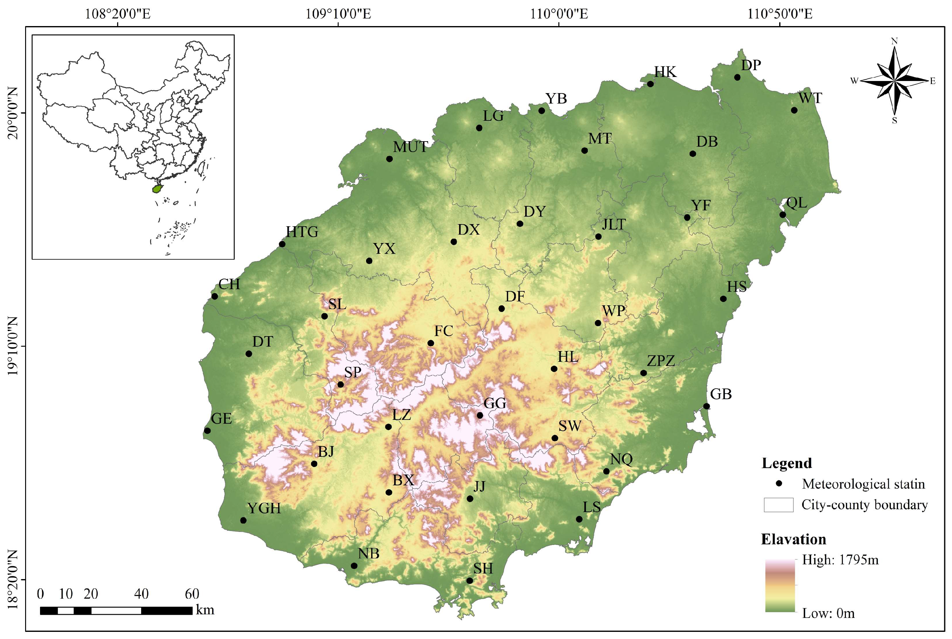
2.1. Study Area

The study area was Hainan Island in southern China (Figure 1), which is China’s largest tropical island, with an area of 33,900 km²; it is approximately located between the latitudes 18°10′ and 20°10′ N and the longitudes 108°37′ and 111°03′ E Bai et al., 2023 [47]. The topography of Hainan Island consists of mountains, hills, plateaus, and plains, with an obvious ladder structure. The terrain of the island exhibits high and low patterns on all sides south of the center, and the altitude of the terrain ranges between 0 and 1795 m. The soil types include lateritic soil, lateritic red soil, and brick yellow soil, with lateritic red soil being the most common. This area is part of the northern edge of the tropics and is influenced by the typical tropical oceanic monsoon climate. The island has a long summer and no winter, and the average annual temperature is 22–27 °C. Rainfall is abundant, with the average annual rainfall ranging from 1000 to 2500 mm Geng et al., 2022 [48], and the rainy and dry seasons are distinct. The rainfall decreases spatially from east to west and is most concentrated during the typhoon period (from May to October). The land cover types are diverse and mainly include forest, agricultural land, and grassland. Due to accelerated urbanization, large-scale deforestation, and other human activities that have interfered with and destroyed the landscape, coupled with frequent extreme rainfall, the risk of soil erosion has increased in this region.

2.2. Data

2.2.1. Daily Rainfall Data

The rainfall data in this study were the daily rainfall data collected at 38 meteorological stations on Hainan Island for the half-century from 1971 to 2020. The rainfall data were collected via siphon-recording rain gauges, which were provided by the Hydrographic Water Resources Survey Bureau of Hainan Province. The observation time of all meteorological stations was the same as the research time. Please refer to the attachment for basic information about the meteorological stations.

2.2.2. ENSO Indicators

ENSO is a naturally occurring anomaly in the ocean and involves atmospheric coupling in the tropical Pacific Ocean. Its two extreme stages are divided according to the following criteria: the abnormal sea surface temperature (SST) fluctuation range exceeds 0.5 °C, and the duration exceeds 5 months. El Niño occurs when the abnormal SST increase is ≥0.5 °C. La Niña occurs when the decrease in the abnormal SST is ≥0.5 °C Wang et al., 2023 [49]. In this study, the MEI Pompa-García et al., 2015 [50], SOI Espinoza et al., 2023 [51], and ONI Zhou et al., 2020 [52] were utilized to reflect the changes in ENSO. These climate indices were based on monthly data from the period 1971–2020 obtained from the National Oceanic and Atmospheric Administration (NOAA) data platform.

2.3. Methods

2.3.1. Calculation of the RE

Previous studies have shown that the accuracy of RE calculation with models based on daily rainfall is greater than that of models based on annual and monthly rainfall Lu et al., 2023; Rutebuka et al., 2020 [53,54]. Due to the lack of data on rainfall events in the study area, the daily rainfall for the calculation of rainfall erosivity was selected in this study according to the principle of the optimal temporal resolution of available rainfall data so as to ensure higher calculation accuracy. Referring to previous studies Zhang et al., 2002; Chen et al., 2017 [5,55], the common calculation model for rainfall erosivity based on daily rainfall is as follows:

Model 1: The CREAMS model Knisei et al., 1980 [17]. This model is calculated as follows:

$${RE}_{\mathrm{h}}=1.03P_i^{1.51}$$

(1)

where RE_h is the RE of the h-th month of one year in MJ·mm·ha⁻¹·h⁻¹, and P_i is the daily rainfall on the i-th day of the h-th month in mm. The model classifies rainfall of 12.7 mm or more as daily erosive rainfall.

Model 2: This model was established by Alves et al., 2022 [56]. This model is calculated as follows:

$$R_i=\alpha [1+\eta \cos (2\pi fj-\omega \left)\right]P_i^{\beta }$$

(2)

where R_i is the RE of the i-th day in MJ·mm·ha⁻¹·h⁻¹; P_i is the erosive rainfall of the i-th day in mm; α, η, ω, and β are all calculated parameters of the model, in which the variation amplitude of α is related to η, ω is the periodic parameter of the maximum cumulative RE, and β is the nonlinear modeling parameter of daily rainfall and its corresponding RE. In addition, f = 1/24, where j is the j-th half-month of the year. The half-month period is divided by the 15th day of each month; the first 15 days constitute a half-month period, and the remainder of the month is the next half-month period, so the whole year is separated into 24 periods. The monthly RE is calculated by summing the daily RE, and the annual RE is calculated by summing the daily RE throughout the year. The model classifies rainfall of 12 mm or more as daily erosive rainfall.

Model 3: This model was modified by Zhang et al., 2002 [5] based on the daily rainfall erosivity model of Richardson et al. 1983 [57]. This model is calculated as follows:

$${RE}_{\mathrm{h}}=\alpha {\sum }_{i=1}^m {\left(p_i\right)}^{\beta }$$

(3)

where

$$\alpha =21.586{\beta }^{-7.1891}$$

(4)

$$\beta =0.8363+{\displaystyle \frac{18.144}{p_{d12}}}+{\displaystyle \frac{24.455}{p_{y12}}}$$

(5)

where RE_h is the RE of the h-th half-month in MJ·mm·ha⁻¹·h⁻¹; m is the number of days within the h-th half-month; P_i is the erosive rainfall on the i-th day within the h-th half-month in mm; α and β are the calculation parameters of the model. P_d12 is the average daily rainfall that is ≥12 mm. P_y12 is the average annual rainfall with daily rainfall that is ≥12 mm (mm). The method of delineating the semilunar period is consistent with that of Model 2. The cumulative erosivity of all semimonthly rainfall in each month is calculated as the monthly RE, and the cumulative erosivity of all semimonthly rainfall in each year is calculated as the annual RE. This model classifies rainfall of 12 mm or more as daily erosive rainfall.

Model 4: This model was established by Shi et al. 2006 [18]. This model is calculated as follows:

$${RE}_h=0.429\left[1+0.328\sin \left({\displaystyle \frac{\pi }{12}}(h-1)\right)\right]{\sum }_{k=1}^n P_i^{1.47}$$

(6)

where RE_h is the monthly RE in MJ·mm·ha⁻¹·h⁻¹. P_i is the daily rainfall on the i-th day of the month in mm. This model classifies rainfall of 12 mm or more as daily erosive rainfall.

Model 5: This model was modified by Xie et al. 2000 [19] and is calculated as follows:

$${RE}_{\mathrm{h}}=0.184{\sum }_{i=1}^m {\left(P_d{I}_{10d}\right)}_i$$

(7)

where RE_h is the RE of the h-th half-month in MJ·mm·ha⁻¹·h⁻¹; m is the number of days within the h-th half-month; P_d is the daily rainfall in mm; I_10d is the maximum rainfall intensity in 10 min per day (mm∙h⁻¹). i indicates the i-th day of the h-th half-month. The method of delineating the semimonthly period and the calculation method for the monthly and annual RE are consistent with those of Model 3. The model similarly classifies rainfall of 12 mm or more as daily erosion rainfall.

2.3.2. Evaluation of the Suitability of the RE Models

Since the parameters of different daily rainfall models are modified and improved according to the rainfall characteristics of different regions established at the beginning, the applicability of each model in different study areas and the reliability of the calculation results are different. To better estimate the RE of Hainan Island, the applicability of the proposed calculation model was evaluated to aid in the selection of the most suitable RE calculation model for accurately calculating the specific type of results. In the applicability evaluation of the calculation model, the effective coefficient (E_f) and relative deviation coefficient (E_r) of the models were used as evaluation indices Cui et al., 2023 [58] to evaluate the accuracy of the calculation results. The evaluation indicators are calculated as follows:

$$E_f=1-{\displaystyle \frac{\sum {\left({RE}_{obs}-{RE}_{\mathrm{oal} }\right)}^2}{\sum {\left({RE}_{obs}-{RE}_{\mathrm{oalm} }\right)}^2}}$$

(8)

$$E_r={\displaystyle \frac{\left|{RE}_{\mathrm{obsn} }-{RE}_{\mathrm{oalm} }\right|}{{RE}_{\mathrm{oalm} }}}$$

(9)

where RE_obs is the annual RE calculated by each model in MJ·mm·ha⁻¹·h⁻¹; RE_oal is the baseline annual RE in MJ·mm·ha⁻¹·h⁻¹; RE_oalm is the average of the baseline multiyear RE in MJ·mm·ha⁻¹·h⁻¹; RE_obsn is the model-calculated multiyear average RE in MJ·mm·ha⁻¹·h⁻¹.

The baseline annual RE was the average of the annual RE calculated with the five models, while the baseline multiyear average RE was the average of the multiyear average RE calculated with each model. The value range of the model effective coefficient was −1–1, and the larger the value was, the more accurate the model calculation result. The relative deviation coefficient ranged from 0 to 1, and the smaller the calculated value was, the more accurate the calculation result of the model Coşkun et al., 2023 [59].

2.3.3. Spatial Interpolation Analysis Method

The spatial interpolation of RE at the 38 sites was used to determine the distributions of rainfall, erosive rainfall, and RE on Hainan Island. The above work was conducted in the ArcGIS 10.8 platform.

Common spatial interpolation methods include the regularized spline (RS), inverse distance weighting (IDW), nearest neighbor (NN), universal kriging (UK), universal cokriging (UCK), ordinary kriging (OK), and ordinary cokriging (OCK) methods. In previous studies, Zhu et al. 2019 [44] used a cross-validation method to evaluate the interpolation effects of the above seven methods. Among these methods, the IDW interpolation method has been found to have the lowest average relative error and average deviation but the highest average prediction accuracy, indicating that the interpolation accuracy of this method was higher. Therefore, this study used the IDW method for spatial interpolation analysis.

IDW interpolation ignores any spatial relationship except for incidental distance based on the principle that the closer things are, the more similar they are. In the interpolation process, a region that is closer to the interpolation point is given more weight, and a region that is farther away is given less weight.

2.3.4. Time-Series Change Analysis Method

In this study, the modified Mann–Kendall (MMK) test Kyaw et al., 2023 [60] was used to analyze the change trends in rainfall, erosive rainfall, and RE in the study area. The MK test method is optimized based on the Mann–Kendall (MK) test method Ahmadi et al., 2022 [61]. It is a common nonparametric testing technique for estimating the change trend of a time series and can reveal the change trend of a time series and its significance. Compared with the MK method, the MMK method, which has been widely used, can eliminate the autocorrelation components of hydrology, rainfall, and other time-series data and improve the reliability of trend test results Zhang et al., 2016; Alashan et al., 2020; Nkunzimana et al., 2021 [62,63,64]. Please refer to Liu et al. 2018 [7] for the specific formula and process for MMK detection.

In addition to the MMK trend test analysis, we also used cross-wavelet transformation analysis (XWT), bivariate wavelet coherence analysis (WTC), and multiple-wavelet coherence analysis (MWC) to explore the effects of single or multiple factors (MEI, SOI, and ONI) on the RE series at different time scales. The XWT can be used to analyze the energy resonance and covariance distribution law of two sets of sequences in the time domain and frequency domain, in addition to revealing the consistency and correlation of the frequency period of two sets of sequences at different time scales, and it can be employed to calculate the phase relationship in the time–frequency space through wavelet phase angle analysis. The WTC is based on a series of automatic wavelet and cross-wavelet energy profiles to analyze the coherence of two sequences by calculating the wavelet coherence coefficients at different time scales, and the MWC is a special form of wavelet coherence used to explore the coherence of more than two sequences. Yu et al. 2015 [65] presented the specific theory and process of the cross-wavelet, and Hu et al. 2017 [66] and Su et al. 2019 [67] presented wavelet coherence analysis and multivariate wavelet coherence analysis, respectively.

2.3.5. Correlation Analysis Method

The potential relationship between ENSO and RE can be further explored through correlation analysis Lee et al., 2023b [68]. To explore the association between RE and ENSO, this study used RE as the dependent variable and the MEI, SOI, and ONI factors characterizing. ENSO as independent variables, and it determined the differences in correlations among the different extreme stages of ENSO.

3. Results

3.1. Evaluation of the Suitability of the RE Calculation Models

The suitability evaluation results for each model for Hainan Island are shown in

Table 1. The results of the evaluation of the suitability of the models.

Parameters	Calculation Models of RE
	Model 1	Model 2	Model 3	Model 4	Model 5
Annual average RE (MJ·mm·ha−1·h−1)	18,021.10	17,354.09	1580.76	12,664.37	16,735.37
Standard deviation (mm)	4498.62	4320.15	3025.89	2731.11	3562.90
Coefficient of variation (Cv)	0.52	0.55	0.27	0.30	0.43
Effectiveness coefficient (Ef)	0.24	0.36	0.81	−0.15	−0.14
Relative deviation coefficient (Er)	0.26	0.41	0.08	0.60	0.35

. Among the results calculated for all models, the maximum annual RE was 18,021.10 MJ·mm·ha⁻¹·h⁻¹, and the minimum was 12,664.37 MJ·mm·ha⁻¹·h⁻¹, which were calculated with Model 1 and Model 4, respectively. The former was 1.42 times greater than the latter. The results of different RE models in the same area were quite different, which may greatly affect the precision of soil erosion prediction and further justify the necessity of evaluating the model applicability. Model 1 had the largest standard deviation, while Model 4 had the smallest standard deviation, indicating that the former had the highest degree of dispersion of calculation results, while the latter had the lowest degree. Among the five models, Model 3 had the smallest deviation coefficient, which indicated that the stability of that model was the highest. In addition, the effective coefficient of Model 3 was greater than that of the other models, reaching 0.81, which indicated that Model 3 was also the most accurate model. Furthermore, the coefficient of the relative deviation of Model 3 was small at only 0.08. In summary, Model 3 was suitable for Hainan Island. Therefore, that model was selected to calculate the RE of Hainan Island from 1971 to 2020.

3.2. Change in RE

3.2.1. Relationships among Rainfall, Erosive Rainfall, and RE

Both rainfall and erosive rainfall on Hainan Island varied considerably over the years from 1971 to 2020. The rainfall ranged from 1177.97 to 2267.21 mm, with a mean value of 1763.82 mm. A daily rainfall of 12 mm was used as the identification standard for erosive rainfall, based on which erosive rainfall was screened and summarized. The statistical analysis revealed that the average erosive rainfall on Hainan Island over the last 50 years reached 1475.19 mm, with a maximum value of 1978.70 mm and a minimum value of 917.93 mm. The ratio of erosive rainfall to rainfall ranged from 77.92% to 87.27%, with an average ratio of 83.63%, indicating that rainfall created a high erosion risk for the soil in this area. According to the results of the correlation analysis (

Table 2. Correlations among the average annual rainfall, average annual erosive rainfall, and average annual RE at each meteorological station.

No.	Station	R with ER	R with RE	ER with RE
1	Danxian	0.98 ***	0.87 ***	0.91 ***
2	Mutang	0.93 ***	0.80 ***	0.87 ***
3	Lingao	0.98 ***	0.88 ***	0.92 ***
4	Yubao	0.94 ***	0.83 ***	0.90 ***
5	Fucai	0.94 ***	0.84 ***	0.89 ***
6	Dafeng	0.96 ***	0.85 ***	0.90 ***
7	Dunya	0.97 ***	0.86 ***	0.92 ***
8	Meiting	0.93 ***	0.82 ***	0.85 ***
9	Jialetan	0.95 ***	0.83 ***	0.89 ***
10	Yongfeng	0.92 ***	0.79 ***	0.82 ***
11	Dabao	0.92 ***	0.80 ***	0.84 ***
12	Haikou	0.98 ***	0.86 ***	0.93 ***
13	Dongpo	0.95 ***	0.87 ***	0.90 ***
14	Wengtian	0.93 ***	0.84 ***	0.91 ***
15	Qinglan	0.98 ***	0.88 ***	0.92 ***
16	Heshui	0.93 ***	0.80 ***	0.82 ***
17	Shenwang	0.95 ***	0.81 ***	0.88 ***
18	Heluo	0.91 ***	0.77 ***	0.80 ***
19	Wupo	0.94 ***	0.83 ***	0.84 ***
20	Zhongpingzai	0.96 ***	0.85 ***	0.91 ***
21	Gangbei	0.96 ***	0.82 ***	0.92 ***
22	Nanqiao	0.93 ***	0.80 ***	0.85 ***
23	Lingshui	0.93 ***	0.79 ***	0.83 ***
24	Jinjiang	0.97 ***	0.89 ***	0.92 ***
25	Songhe	0.98 ***	0.87 ***	0.92 ***
26	Nanbing	0.93 ***	0.80 ***	0.83 ***
27	Yinggehai	0.96 ***	0.85 ***	0.84 ***
28	Ganen	0.96 ***	0.82 ***	0.83 ***
29	Datian	0.94 ***	0.83 ***	0.85 ***
30	Gongguan	0.93 ***	0.79 ***	0.81 ***
31	Lezhong	0.96 ***	0.85 ***	0.87 ***
32	Baoxian	0.93 ***	0.78 ***	0.85 ***
33	Baojie	0.94 ***	0.83 ***	0.82 ***
34	Sanpai	0.97 ***	0.86 ***	0.93 ***
35	Shilu	0.93 ***	0.81 ***	0.85 ***
36	Changhua	0.92 ***	0.78 ***	0.86 ***
37	Haitougang	0.95 ***	0.82 ***	0.87 ***
38	Yaxing	0.96 ***	0.85 ***	0.90 ***
Mean	-	0.95	0.83	0.87

R is the rainfall, ER is the erosive rainfall, and RE is the RE. *** indicates a 99% confidence level.

), the mean correlation coefficient between rainfall and erosive rainfall for the 38 stations was 0.95, the mean correlation coefficient between rainfall and RE was 0.83, and the mean correlation coefficient between erosive rainfall and RE was 0.87. RE had a high correlation with rainfall and erosive rainfall, and the correlation was most significant with erosive rainfall. All of the data passed the 99% confidence test, indicating the reliability of the correlation test results.

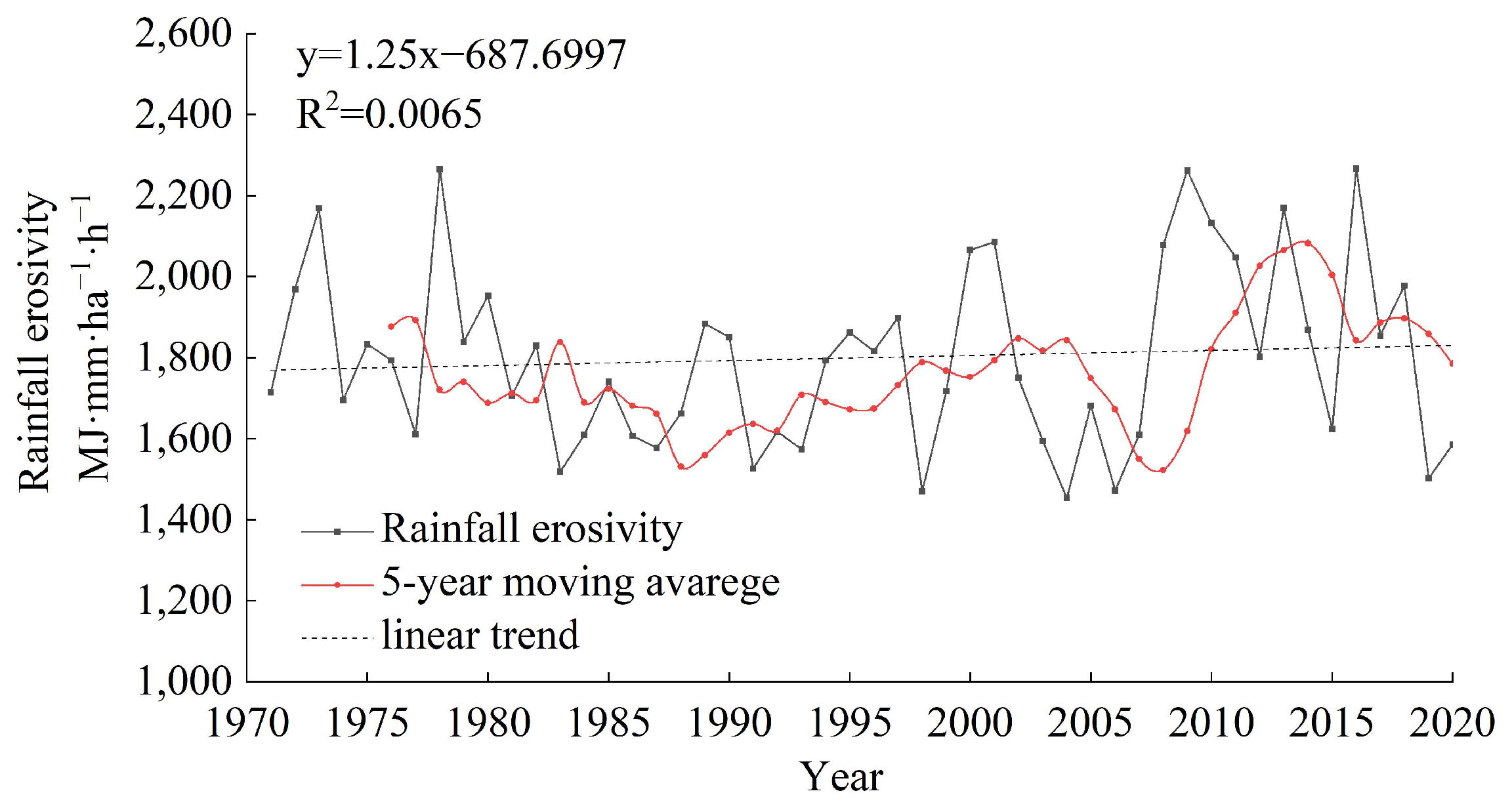
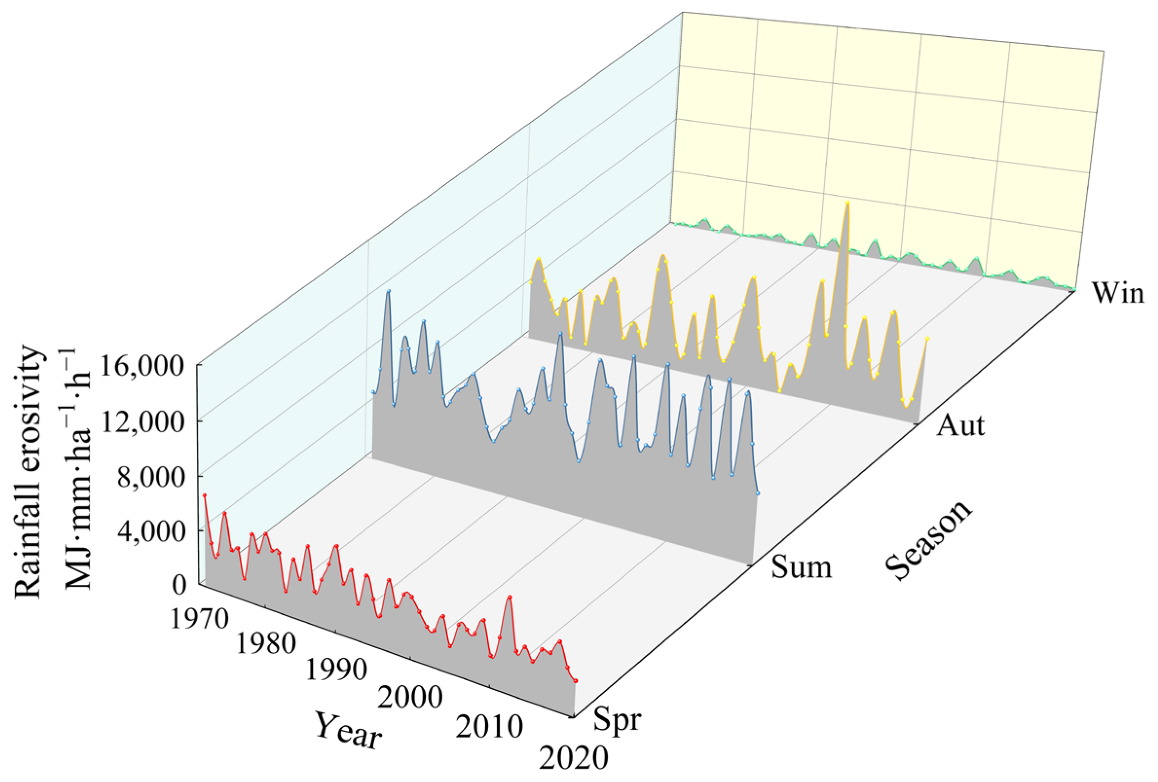
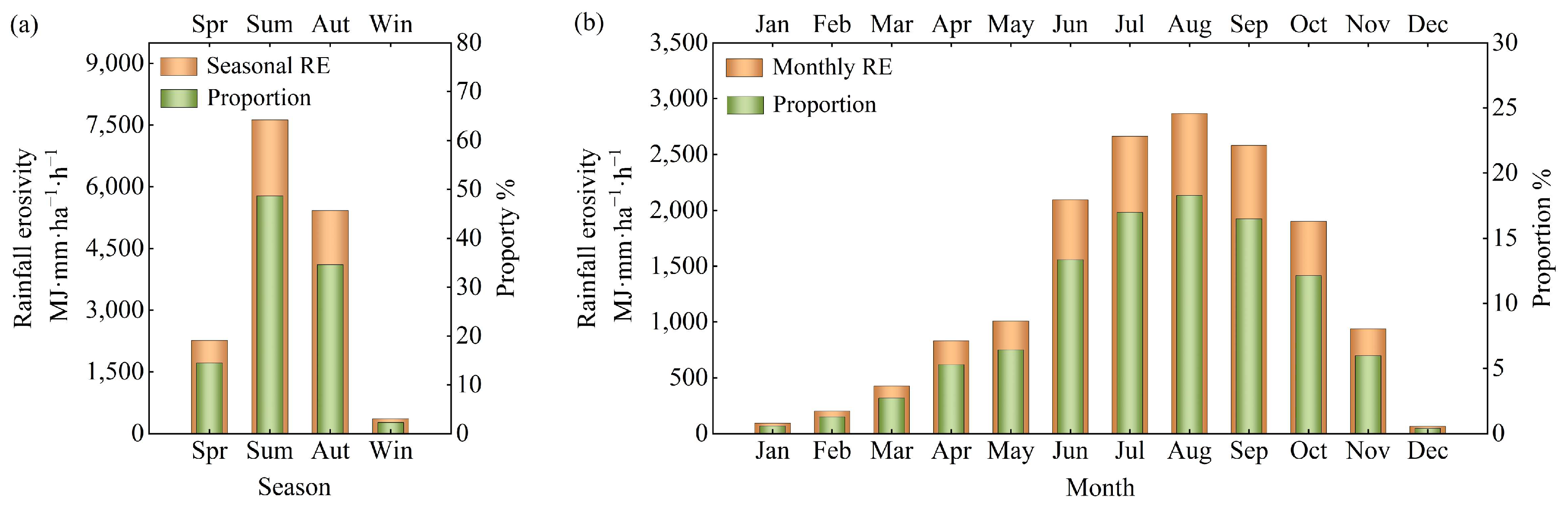
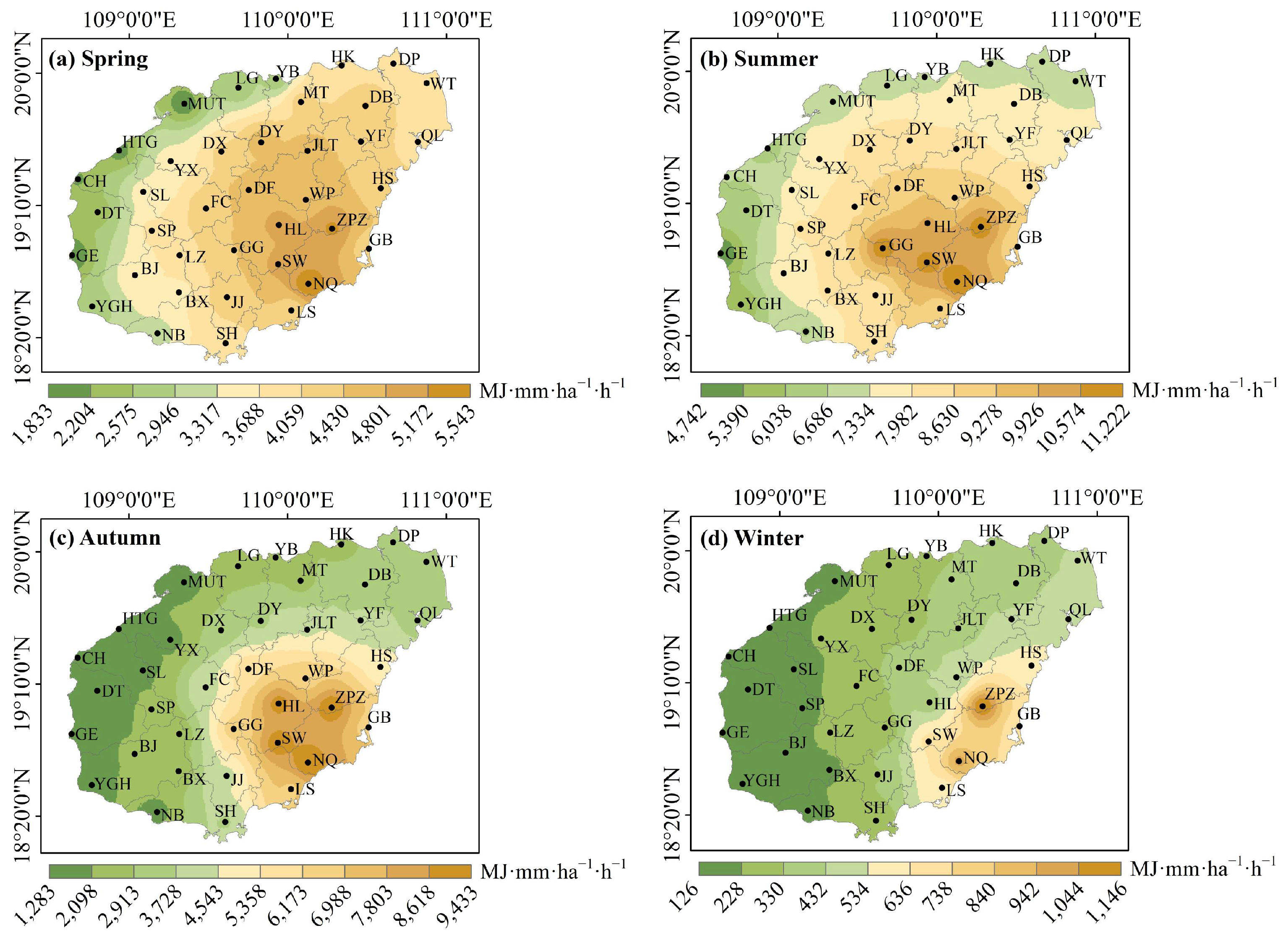
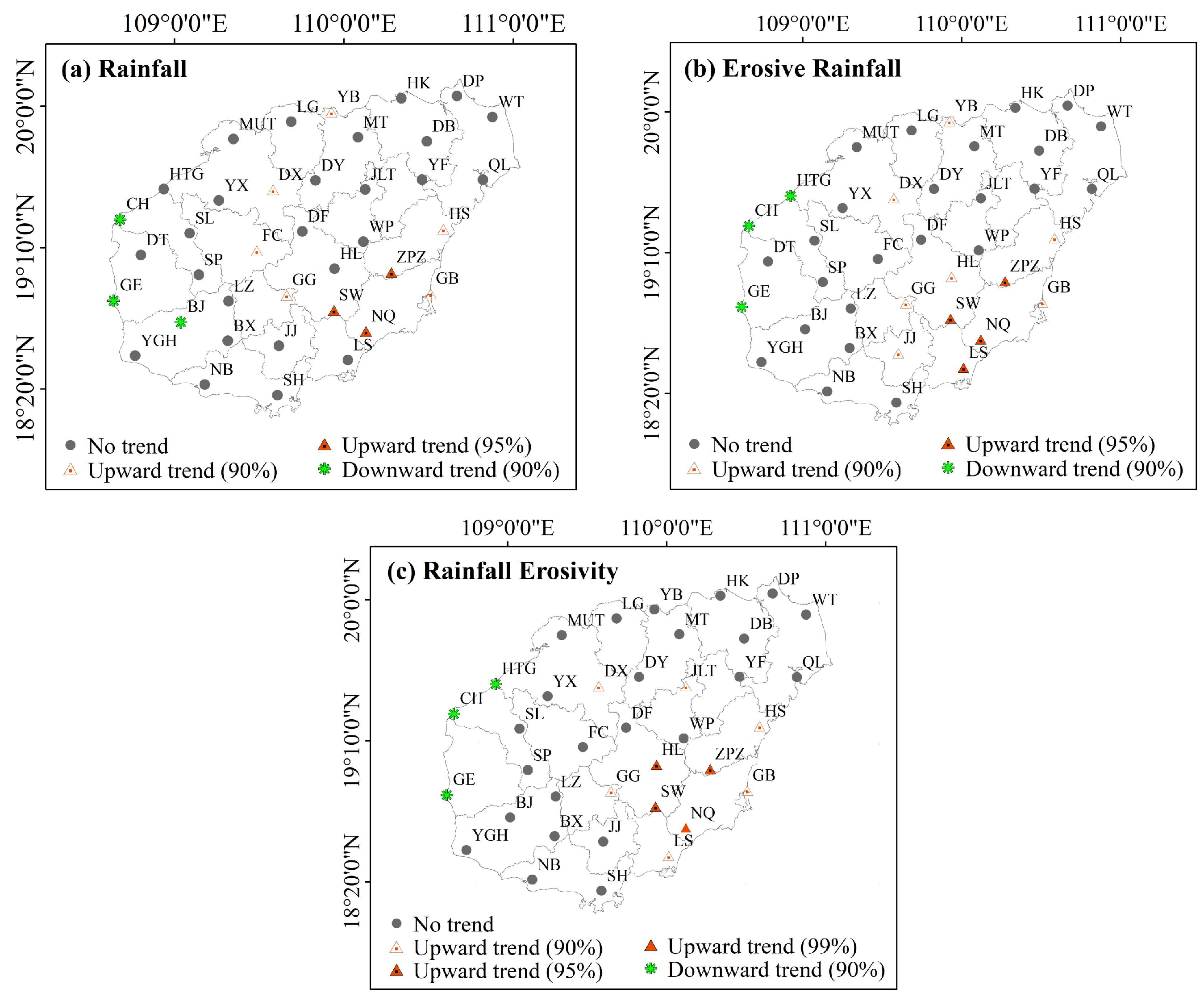
3.2.2. Spatiotemporal Variation in RE

Over the last 50 years, the average annual RE on Hainan Island was 15,671.28 MJ·mm·ha⁻¹·h⁻¹, with the maximum occurring in 2016 (22,935.76 MJ·mm·ha⁻¹·h⁻¹) and the minimum occurring in 1987 (8584.42 MJ·mm·ha⁻¹·h⁻¹). The results of the experiment showed that the RE had a fluctuating and increasing tendency, with an average annual variation of 42.26 MJ·mm·ha⁻¹·h⁻¹ (Figure 2). The RE trend can be divided into three phases: the fluctuation decreased from 1971 to 1987 and increased from 1988 to 2003, and the fluctuation amplitude was the most obvious from 2004 to 2020, showing a decreasing trend. There were great discrepancies in the seasonal RE; summer (from June to August) had the largest RE, which was 7622.51 MJ·mm·ha⁻¹·h⁻¹, making up 48.64% of the year, followed by autumn (from September to November), which was 5421.17 MJ·mm·ha⁻¹·h⁻¹, making up 34.59% of the year. Winter (from December to February of the following year) accounted for the smallest proportion at only 2.31% (Figure 3 and Figure 4a).

The spatial characteristics of the annual RE at the 38 stations were obtained via interpolation. Overall, the RE exhibited an obvious gradient pattern, and the distribution was the same as that of the rainfall and erosion rainfall, which decreased from east to west. The RE distribution pattern was more similar to that of erosive rainfall (Figure 5), which was consistent with the results of the correlation analysis. Considering the seasonal differences, the spatial characteristics of RE in each season were analyzed (Figure 6). The distribution patterns of the seasonal and annual RE were basically the same, showing a decreasing tendency from east to west. Notably, in summer, the RE of 68.42% of the sites reached 7334 MJ·mm·ha⁻¹·h⁻¹. In addition to the 12 sites and some areas in the west, most of the interpolation areas of the island were greatly affected by rainfall erosion. In particular, the cities of Wanning and Qiongzhong on southeastern Hainan Island were the main distribution areas of maximum rainfall and RE, and the mean annual RE reached more than 22,000 MJ·mm·ha⁻¹·h⁻¹. Notably, most of the terrain in this region is mountainous, which leads to a high potential risk of soil erosion and flood disasters Olorunfemi et al., 2020 [69]. Attention should be given to soil and water conservation in this region.

As shown in

Table 3. Mann–Kendall trend test results for annual rainfall, erosive rainfall, and RE at various stations.

No.	Station	Rainfall (mm)	Erosive Rainfall (mm)	RE (MJ·mm·ha−1·h−1)
1	Danxian	4.43 *	4.86 *	50.78 *
2	Mutang	7.39	−7.30	−200.14
3	Lingao	4.77	5.06	92.39
4	Yubao	11.48 *	10.00 *	64.10
5	Fucai	1.73 *	−1.78	−35.72
6	Dafeng	−5.80	−5.63	−67.39
7	Dunya	5.09	5.57	67.25
8	Meiting	2.82	3.02	49.11
9	Jialetan	−0.17	0.35	7.20 *
10	Yongfeng	0.57	−0.43	25.27
11	Dabao	2.62	2.01	65.34
12	Haikou	0.88	1.54	46.43
13	Dongpo	4.21	3.07	16.60
14	Wengtian	−5.22	−5.21	−47.53
15	Qinglan	−3.41	−3.11	−53.52
16	Heshui	3.04 *	2.31 *	38.50 *
17	Shenwang	4.43 **	3.16 **	31.14 **
18	Heluo	−0.46	0.42 *	3.84 **
19	Wupo	5.03	4.02	55.06
20	Zhongpingzai	0.79 **	0.80 **	−30.94 **
21	Gangbei	5.57 *	4.16 *	28.21 *
22	Nanqiao	12.79 **	13.43 **	187.26 ***
23	Lingshui	2.56	2.89 **	24.88 *
24	Jinjiang	2.59	4.58 *	58.56
25	Songhe	7.53	8.22	126.61
26	Nanbing	−0.54	0.80	−10.22
27	YingGeHai	2.38	2.61	−4.15
28	Ganen	−4.33 *	−4.38 *	−49.46 *
29	Datian	7.02	−7.20	100.82
30	Gongguan	0.28 *	0.55 *	24.74 *
31	Lezhong	4.47	4.85	30.15
32	Baoxian	6.43	5.44	43.59
33	Baojie	−3.67 *	−3.91	−32.88
34	Sanpai	2.14	2.97	46.16
35	Shilu	−1.07	−1.45	−23.82
36	Changhua	−3.24 *	−2.35 *	−63.16 *
37	Haitougang	−1.00	−1.08 *	−7.88 *
38	Yaxing	0.85	1.61	29.86

* indicates a 90% confidence level for the trend of change, ** indicates a 95% confidence level for the trend of change, *** indicates a 99% confidence level for the trend of change.

, the trend of the rainfall erosive force varied among the sites. The maximum value of decreasing change among the 38 stations was 200.14 MJ·mm·ha⁻¹·h⁻¹, which occurred at Mutang station; the maximum value of increasing change was 187.26 MJ·mm·ha⁻¹·h⁻¹, which occurred at Nanqiao station. More than 60% of the meteorological stations on Hainan Island showed an increasing trend in RE. Among the stations, eleven stations showed a significant upward trend, and three stations showed a significant downward trend with a confidence level of 90%. In terms of spatial distribution, the stations with an increasing trend in RE were concentrated in the southeastern region of Hainan Island, and the stations with a decreasing trend were mainly distributed in the western region, which was basically consistent with the spatial distribution of rainfall and the trend of erosive rainfall (Figure 7).

3.3. Characteristics of the ENSO and Its Effect on RE

3.3.1. Temporal Distribution of Different ENSO Periods

In this study, the ONI of the updated base period was used as an indicator to delineate ENSO events as the El Niño period or the La Niña period. The time between these two climatic periods was defined as the neutral period. El Niño events were defined as abnormal changes in ONI ≥ 0.5 °C, and La Niña events were defined as abnormal changes in ONI ≤ −0.5 °C. Both events were characterized by abnormal index values lasting for at least five consecutive months. During the research period of nearly 50 years, a total of 29 extreme weather periods occurred, including 14 El Niño events and 15 La Niña events (

Table 4. Time-series distributions of El Niño and La Niña events during the period 1971–2020.

No.	Climate Events	Time Interval	Duration in Months	Average Monthly RE (MJ·mm·ha−1·h−1)
1	La Niña	1971.01–1972.01	13	1238.59
2	El Niño	1972.05–1973.03	11	1828.15
3	La Niña	1973.05–1974.07	15	1566.05
4	La Niña	1974.10–1976.03	18	1025.16
5	El Niño	1976.09–1977.02	6	2033.39
6	El Niño	1977.09–1978.01	5	970.70
7	El Niño	1982.05–1983.06	14	1173.38
8	La Niña	1984.10–1985.06	9	580.76
9	El Niño	1986.09–1988.02	18	820.94
10	La Niña	1988.05–1989.05	13	1126.87
11	El Niño	1991.06–1992.06	13	1384.28
12	El Niño	1994.09–1995.03	7	941.24
13	La Niña	1995.08–1996.03	8	1528.90
14	El Niño	1997.05–1998.04	12	1095.89
15	La Niña	1998.07–2001.02	32	1310.41
16	El Niño	2002.06–2003.02	9	1432.35
17	El Niño	2004.08–2005.02	7	2334.50
18	La Niña	2005.11–2006.03	5	298.74
19	El Niño	2006.09–2007.01	5	1305.12
20	La Niña	2007.07–2008.06	12	1126.46
21	La Niña	2008.11–2009.03	5	490.14
22	El Niño	2009.08–2010.03	8	1849.70
23	La Niña	2010.06–2011.05	12	1489.59
24	La Niña	2011.08–2012.03	8	1666.49
25	El Niño	2015.03–2016.04	14	1038.44
26	La Niña	2016.08–2016.12	5	1469.98
27	La Niña	2017.10–2018.04	7	939.39
28	El Niño	2018.10–2019.05	8	1298.30
29	La Niña	2020.08–2020.12	5	1922.96
Mean RE in El Niño				1393.31
Mean RE in La Niña				1185.37
Mean RE in ENSO				1285.75
Mean RE in Neutral period				1349.67
Mean RE during the period 1971–2020				1306.02

).

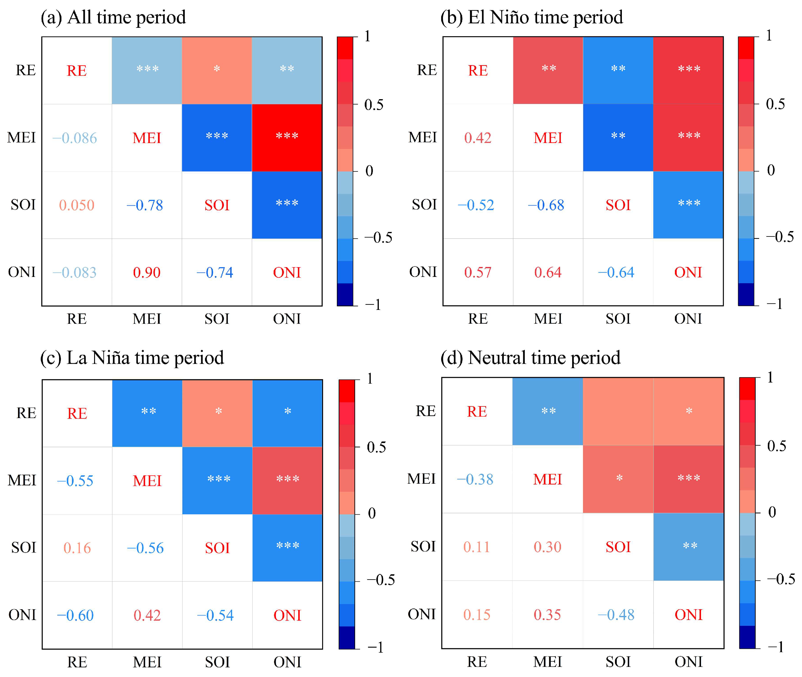
3.3.2. Correlation between RE and the ENSO

There were differences in the monthly RE in each stage of the El Niño and La Niña periods (Table 4). During the El Niño period, the maximum and minimum mean monthly RE values were 2334.50 MJ·mm·ha⁻¹·h⁻¹ and 820.94 MJ·mm·ha⁻¹·h⁻¹, respectively, with a ratio of 2.84. The maximum and minimum average monthly RE values during La Niña were 1922.96 MJ·mm·ha⁻¹·h⁻¹ and 298.74 MJ·mm·ha⁻¹·h⁻¹, respectively, with a ratio of 6.43. The variability in the RE during La Niña events was higher than that during El Niño events. The mean monthly RE during El Niño was 1393.31 MJ·mm·ha⁻¹·h⁻¹, which was higher than the value of 1185.37 MJ·mm·ha⁻¹·h⁻¹ during La Niña, and the average monthly RE during the period 1971–2020 was between those of the above two periods. This result shows that the risk of erosion caused by erosive rainfall was more serious during the El Niño stage and less serious during the La Niña stage. During the ENSO, the average monthly RE was 1285.75 MJ·mm·ha⁻¹·h⁻¹, which was lower than the value of 1349.67 MJ·mm·ha⁻¹·h⁻¹ in the neutral period and the value in the whole study period. We found that under the influence of ENSO, the RE on Hainan Island was gradually weakened, and the risk of soil erosion caused by rainfall decreased during this period. Through correlation analysis between the RE and the MEI, SOI, and ONI, the relationships between the RE and ENSO characterization parameters in the four periods (Figure 8a), the El Niño period (Figure 8b), the La Niña period (Figure 8c), and the neutral period (Figure 8d) were further explored to distinguish the characteristics of the different extreme climate periods. During the whole study period, the association between RE and the MEI was negative, which also occurred between RE and the ONI. The confidence interval of the above correlation reached 95%. The RE was found to be weakened under the influence of the MEI and ONI, which was consistent with the findings in Table 3. During El Niño, RE was significantly associated with the MEI, SOI, and ONI. The association between RE and the ONI was the strongest, with a correlation coefficient of 0.57 and a significance level of p = 0.01, followed by that between RE and the MEI, with a correlation coefficient of 0.42 (p = 0.05). In contrast to the MEI and ONI, the correlation of RE with the SOI was negative, with a correlation coefficient of −0.52 (p = 0.05). During La Niña, RE was negatively correlated with both the MEI and ONI; the correlation coefficient with the MEI was −0.55 (p = 0.05), and that with the ONI is −0.60 (p = 0.1). The opposite pattern occurred during El Niño. In addition, the association between the RE and the SOI during La Niña was weak at only 0.16 (p = 0.1). In contrast, the RE during this period had a greater correlation with the MEI and ONI. In the neutral period, the association between RE and the SOI was not obvious. However, RE was negatively associated with the MEI (p = 0.05) and positively correlated with the ONI (p = 0.1).

The correlation between RE and the MEI at the 38 research stations was as follows: there were 18 stations with extremely significant correlations with the MEI (p = 0.01), which were mainly found in the eastern and southeastern regions of Hainan Island (Figure 9). Furthermore, there were five stations with significant correlations with the MEI (p = 0.05), and there was no centralized distribution. The association between RE and the SOI at all stations was weaker than that with the MEI. There were only three stations with extremely significant correlations with the SOI (p = 0.01), which were concentrated in the southeastern part of Hainan Island, and 18 stations had significant correlations (p = 0.05), which were mainly found in the southern and northeastern parts of Hainan Island. Among the correlations between the RE and the ONI, there were 9 stations with extremely significant correlations and 16 stations with significant correlations. The stations with extremely significant correlations were concentrated in the eastern part of Hainan Island, while the stations with significant correlations were in the southern and northeastern parts of Hainan Island. In summary, stations with significant correlations between RE and each ENSO index were mostly concentrated east of Hainan Island, while stations west of Hainan Island had no significant correlation characteristics. Among the 38 stations, the proportion of stations with significant associations between RE and the MEI, SOI, and ONI was greater than 55%, but the proportion of stations with very significant correlations was the highest, reaching 47.37%.

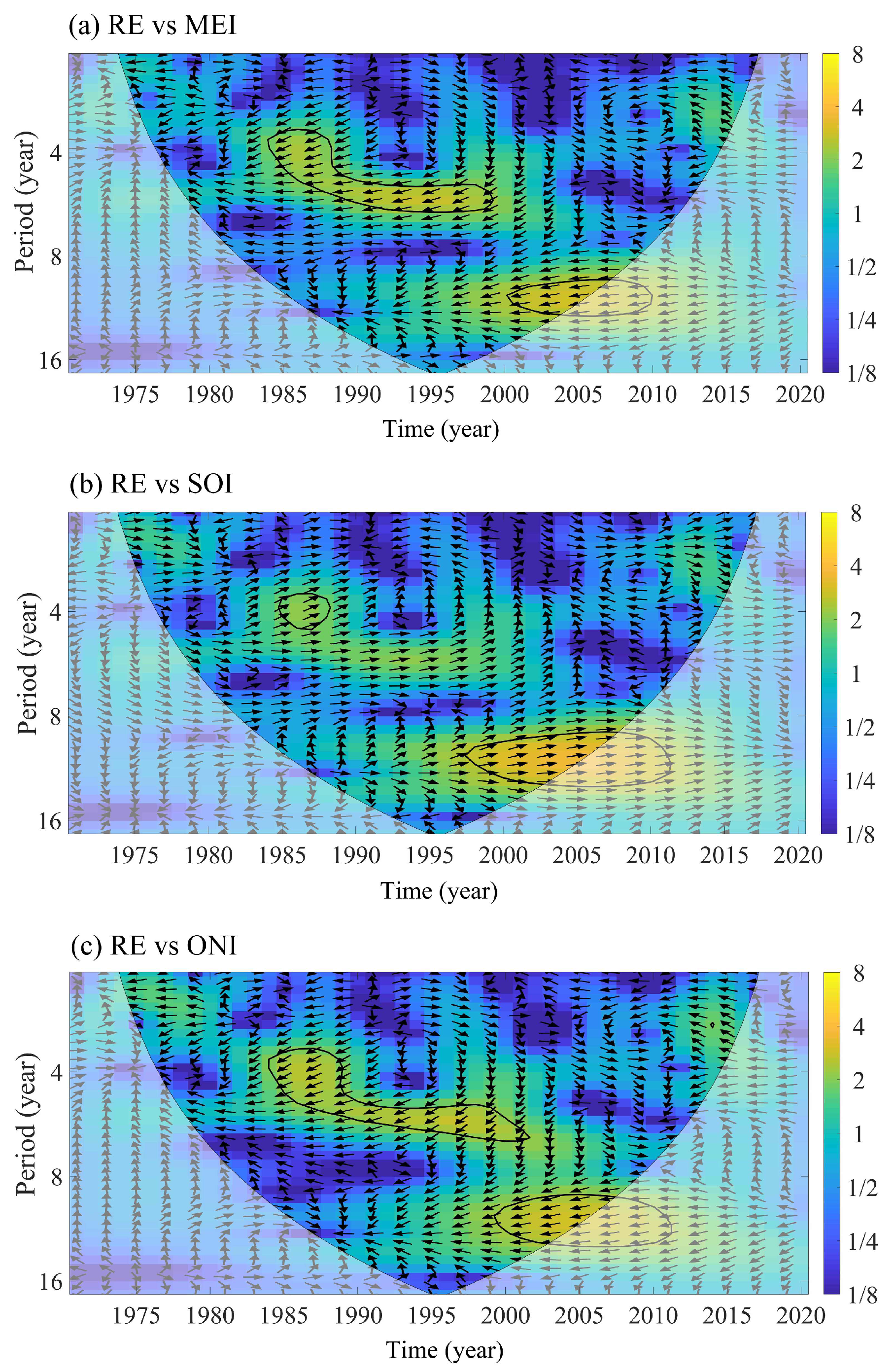
3.3.3. Effect of the ENSO on RE

Based on cross-wavelet analysis, cross-wavelet power graphs of RE and the MEI (Figure 10a), SOI (Figure 10b), and ONI (Figure 10c) were generated. In the figure, the region within the solid line passed the red noise standard general test with 95% confidence, and the thin arc region represents the effective spectral value of the wavelet influence in the vertebra Grinsted et al., 2004; Thomas et al., 2022 [70,71]. There were two significant resonance stages between the RE and the MEI on Hainan Island, and the corresponding periods were 1984–1999 and 2000–2007. The resonant periods were 3–6 years and 9–11 years, respectively (Figure 10). The arrow in the region with the solid line points to the lower left, indicating that RE and the MEI were in a reversed phase; the two were significantly negatively correlated, and RE lagged behind the MEI. According to the average phase angle, it can be inferred that the RE lagged behind the MEI by approximately 1.98 years and 4.43 years during the periods 1984–1999 and 2000–2007, respectively. Similarly, Figure 10b shows that the arrows in the solid line area basically point to the right, indicating that the RE and the SOI on Hainan Island had the same phase, and the two presented a strong positive correlation. In addition, during the period 1997–2007, the RE and the SOI had a significant resonance relationship on the scale of a 9–12 year cycle. However, during the period 1985–1987, although the two have a resonance period of 3 to 4 years, the cross-wavelet power spectrum energy was low, and there was no strong correlation. In the cross-wavelet power spectra of the RE and the ONI, during the entire study period, there were significant resonance associations between the RE and the ONI in two different periods, namely 1984–2001 and 1999–2006, with resonance periods of 3–6 years and 9–13 years, respectively. In these two resonant periods, the arrows point to the lower left and the left, respectively. The phase of the RE was opposite to that of the ONI, which indicated a strong negative correlation between the two. The RE lagged behind the ONI, and the lag times were approximately 1.5 and 5 years, respectively. According to the results of the cross-wavelet analysis, the MEI, SOI, and ONI exhibited significant correlations and resonance effects with the RE during the entire study period, but there were significant differences in the occurrence time, direction, and intensity.

To further explore the impact of ENSO on RE at different time scales, bivariate wavelet coherence analysis and multivariate wavelet coherence analysis were conducted on the RE of Hainan Island and the MEI, SOI, and ONI (Figure 11 and Figure 12). Figure 11 shows that RE was intimately associated with the single representation index of ENSO. The average wavelet coherence coefficient (AWC) ranged from 0.79 to 0.85, and the percentage area of significant coherence (PASC) ranged from 5.9 to 18.6. Among the RE and MEI values, the AWC and PASC were the highest at 0.85 and 18.6, respectively. The association between RE and the MEI was the greatest. As a joint impact of the two ENSO representation indices, the AWC and PASC ranged from 0.92 to 0.95 and from 3.6 to 19.0, respectively; the AWC and PASC between the combination of RE and the MEI–ONI were the largest (0.95 and 19.0, respectively). Finally, the combined effect of RE and MEI–SOI–ONI was analyzed, and the AWC and PASC were 0.97 and 4.9, respectively (

Table 5. Consistency between the RE and ENSO indices based on wavelet coherence analysis.

Analytical Method	Characteristic Indices of ENSO	AWC	PASC (%)
WTC	MEI	0.85	18.6
	SOI	0.79	5.9
	ONI	0.83	9.1
MWC	MEI-SOI	0.94	3.6
	MEI-ONI	0.95	19.0
	SOI-ONI	0.92	5.7
	MEI-SOI-ONI	0.97	4.9

The AWC and the PASC were used to evaluate the relationships between the RE and the MEI and between the SOI and the ONI. When the increased PASC was greater than 5%, the analytical results of the MWC were significant Yang et al., 2020 [72].

), which were greater than the combined effect of the two factors but still smaller than that in the single-factor analysis. In conclusion, among the ENSO indices and their combinations, the MEI was the main factor influencing RE.

4. Discussion

4.1. Evaluation of the Suitability of the RE Calculation Model

The calculation accuracy of the RE directly affects the application of the soil erosion model, which is crucial for the comprehensive control of regional soil and water loss David et al., 2023 [73]. In previous calculations, the classical model of EI₃₀ was generally used to calculate the rainfall erosion coefficient, which ensured high accuracy, but at the same time, it also had limitations, such as the high-resolution requirements of rainfall observation data and difficult integration processing; thus, the EI₃₀ method cannot be applied to many regions. To solve this problem, many researchers have established RE calculation models on various time scales based on EI₃₀ rainfall data. Among them, Rutebuka et al. 2020 [54] reported that the calculation accuracy of daily RE models was often greater than that of monthly and annual RE models. This result is closely influenced by rainfall characteristics, and different models have different levels of suitability for different regions. In our study, against the background of rainfall in the same research area, the calculation results of the different models were not the same. Chen et al. 2018 [4] directly cited the improved calculation model of Zhang et al. 2002 [5] when studying the abnormal modifications of RE in the southeastern coastal region of China and its correlation with the climate index without comparing the applicability of other models in this region, and the accuracy of their calculation results needs further discussion. In a study of the spatiotemporal RE pattern in Southwest China, Chen et al. 2017 [55] evaluated the suitability of RE calculation models at five different timescales and noted that the monthly rainfall model established by Lu et al. 2006 [74] had the highest accuracy in this region, but the suitability of this model differed among regions. This result further justifies the need for an evaluation of the suitability of the RE calculation model. In this study, five commonly used daily RE models were selected. By analyzing the suitability of each model on Hainan Island, China, the most appropriate RE calculation model was selected to ensure the accuracy of the study results and provide a pivotal reference for the accurate application of the calculation model in the study of RE in this region.

4.2. Characteristics of Variations in RE

The mean annual RE of Hainan Island from 1971 to 2020 was 15,671.28 MJ·mm·ha⁻¹·h⁻¹, which was approximately 4.19 times the mean annual RE of China. These values were greater than those in the southwest karst region Xu et al., 2023 [75], northwest Loess Plateau region Zhang et al., 2022 [76], central and eastern China Wei et al., 20202022 [77], and northeast black soil region Li et al., 2021 [78]. Hainan Island is one of the regions with the highest RE levels in China, which is consistent with the spatial features of high RE in southeastern China and low RE in northwestern China Chen et al., 2020 [11]. Similarly, according to the RE grades determined by Huang et al. 2013 [79], Hainan Island is a highly erosive area, and the potential erosion caused by rainfall is more prominent. In the last 50 years, the RE of Hainan Island has shown a fluctuating upward trend, which is the same as that of Fujian Province in the mid-latitude coastal area Chen et al., 2018 [4]. In reference to the annual distribution, RE is potent in the rainy season (from June to October) and is mainly affected by the East Asian summer monsoon Zhang et al., 2015 [80]. The summer rainfall is more abundant than that in the other three seasons, and 48.64% of the annual RE occurs in summer (from June to August). The frequent occurrence of extreme weather events, such as typhoons, and the consequent increase in rainfall intensity resulted in a surge in the rainfall erosion capacity during this period Chen et al., 2022 [81]. Therefore, extra attention should be given to soil erosion prevention on Hainan Island in summer. The spatial distribution traits of RE are basically the same as those of erosive rainfall, revealing a gradually decreasing tendency from east to west. The high-value area of RE extends from the southeast to the central and eastern mountainous areas, while sufficient warm and humid air brought by tropical monsoons blows westward from the ocean in eastern Hainan Island to the land and is uplifted to form topographic rain when it reaches the mountains in the central and eastern parts of Hainan Island. This phenomenon is more obvious in the summer. Notably, the undulating mountains in rainy areas also provide potential topographic conditions for the occurrence of soil erosion. Under the coupled effects of high RE and topography, the stability of the soil structure is seriously challenged Olorunfemi et al., 2020 [69]. Therefore, attention should be paid to the monitoring and control of natural disasters such as soil erosion and landslides in this area.

RE, as an important parameter of the USLE and RUSLE models, directly affects the soil erosion process. According to the Bulletin of Soil and Water Conservation of China (2021), the area of soil and water loss in China in 2021 was 2,674,200 km², which was 256,700 km² less than that in 2011, a decrease of 8.70%. The soil and water loss areas in the southern hilly area of Hainan Island also showed a downward trend, while the RE in the study area showed an upward tendency. The main factors causing these patterns are human activities, among which soil and water conservation measures and land management are the main relevant factors Zhang et al., 2023 [82]. Future research should focus on the coupled effects of RE and soil erosion under different anthropogenic measures.

4.3. RE Is Affected by ENSO

Studying the effect of ENSO on RE is helpful for revealing the causes of regional RE changes and plays an important role in the proposal of soil erosion and atmospheric disaster prevention strategies. Based on the characteristics of variations in RE, the relationship between RE and ENSO on Hainan Island was studied. We found that the ENSO characterization indices MEI, SOI, and ONI were all significantly correlated with RE on Hainan Island, and this relationship also existed in Guizhou Province Zhu et al., 2019 [44] and Fujian Province Chen et al., 2018 [4]. Among the different climatic phases, the RE is greater in the El Niño period than in the La Niña period, which is mainly because ENSO promotes rainfall and erosive rainfall events in the Northern Hemisphere during the El Niño period Kevin et al., 2019 [83]. However, rainfall in the Northern Hemisphere decreases during the La Niña period, resulting in a reduction in rainfall erosivity Adimasu et al., 2021 [84]. In this study, the mean value of RE during the neutral period was between that during the El Niño period and that during the La Niña period, which further reflects the role of ENSO in RE during different stages. In addition, ENSO is significantly correlated with RE in different stages, and the most significant correlation occurs during the El Nino period, which is different from the results of Zhu et al. 2019 [44]. In the study by Zhu et al., RE was significantly correlated only in the two extreme stages of El Nino and La Nina, while in this study, there was also a significant correlation between the whole period (1971–2020) and the neutral period, which may have been related to differences in the location of the study area. Hainan Island is a tropical island, while Guizhou Province is in an inland plateau area, so Hainan Island is affected by large-scale atmospheric circulation activities triggered by ENSO in a shorter period and without the obstruction of tall mountain terrain, which makes the influence of the feedback of the ENSO in the study area more direct and climate responses, such as rainfall, more sensitive. Regional differences in RE in response to ENSO were also reflected in this study. The correlations between the meteorological stations and the MEI, SOI, and ONI were significantly different. The number of stations with an extremely significant association between RE and the MEI accounted for the greatest proportion, illustrating that the variation in RE on Hainan Island was the most sensitive to the MEI. This result was consistent with those of previous studies Xu et al., 2019; Zhu et al., 2019 [44,85].

Previous studies have mostly focused on the connection between RE and a single factor of ENSO, but the more comprehensive study of the effect of ENSO on RE from the perspective of multifactor combinations in this study is more in-depth than that in previous studies. In the single-factor analysis, the AWC and PASC of the MEI and RE were the largest, indicating that the MEI had the greatest influence on the RE, which further supported the above research results. According to the two-factor analysis with RE, both the AWC and PASC were found to be greater than the single-factor MEI according to the joint MEI–ONI analysis, indicating that the joint MEI–ONI control on RE was more significant, which revealed a relationship that was not found in the correlation analysis Xu et al., 2019; Zhu et al., 2019 [44,85]. In the three-factor analysis with RE, both AWC and PASC were found to be lower than those of the one-factor and two-factor analyses, which coincided with the findings of Zhang et al. 2022 [76]. In summary, the effect of the ENSO on RE was influenced not only by the single effect of the MEI but also by the joint effects of the MEI and ONI. Thus, the MEI and MEI–ONI can be analyzed as key indices in future studies related to ENSO and RE in this study area.

In this study, the influence of ENSO on RE on Hainan Island was explored. However, large-scale atmospheric circulation is a complex process involving multiple factors. The influences of the North Atlantic Oscillation, Pacific Decadal Oscillation, Arctic Oscillation, and tropical cyclones on RE cannot be ignored. Therefore, in future studies, more in-depth research on the effects of the comprehensive action of large-scale climate factors on the changes in and prediction of RE is needed, as it will help fully characterize the impact of atmospheric circulation on our living environment and aid in the development of better coping strategies.

5. Conclusions

In this study, a suitable RE calculation model for the study area was selected through a suitability evaluation. Based on daily rainfall data, the spatiotemporal variation trend of RE on Hainan Island in the last half-century was analyzed. The correlation between ENSO and RE was also investigated, and the individual and joint effects of different ENSO characterization indicators on RE were explored. On Hainan Island, RE showed a fluctuating upward trend, and it was the most concentrated in summer, accounting for 48.64% of the whole year. The spatial distribution pattern of RE was basically consistent with that of rainfall and erosive rainfall, decreasing from east to west. The correlation analysis of RE with the MEI, SOI, and ONI showed that ENSO had a significant effect on RE. The monthly average RE in El Niño periods was greater than that in La Niña periods, while the RE in neutral periods was between the two. The risk of rainfall erosion caused by El Niño periods was greater than that of any other period. Among the ENSO characterization indicators, the MEI and MEI–ONI had the closest influence on RE, as they influenced it separately and jointly. This study further deepened the understanding of ENSO’s impact on RE. The risk of rainfall erosion on Hainan Island is relatively serious, especially during El Niño periods. Future studies can be based on the MEI and MEI–ONI to strengthen the prediction of ENSO’s influence on RE in this region, assess the risk of soil erosion disasters caused by extreme rainfall events, and propose effective and reliable prevention and control strategies in advance to reduce losses caused by disasters.

References

1. Bertol, I.; Schick, J.; Bandeira, D.H.; Paz-Ferreiro, J.; Vázquez, E.V. Multifractal and joint multifractal analysis of water and soil losses from erosion plots: A case study under subtropical conditions in Santa Catarina highlands, Brazil. Geodermia 2017, 287, 116–125. [Google Scholar] [CrossRef]
2. Lai, C.; Chen, X.; Wang, Z.; Wu, X.; Zhao, S.; Wu, X.; Bai, W. Spatio-temporal variation in rainfall erosivity during 1960–2012 in the Pearl River Basin, China. Catena 2016, 137, 382–391. [Google Scholar] [CrossRef]
3. Demissie, S.; Meshesha, D.T.; Adgo, E.; Haregeweyn, N.; Tsunekawa, A.; Ayana, M.; Mulualem, T.; Wubet, A. Effects of soil bund spacing on runoff, soil loss, and soil water content in the Lake Tana Basin of Ethiopia. Agric. Water Manag. 2022, 274, 107926. [Google Scholar] [CrossRef]
4. Chen, S.; Zha, X. Effects of the ENSO on rainfall erosivity in the Fujian Province of southeast China. Sci. Total Environ. 2018, 621, 1378–1388. [Google Scholar] [CrossRef]
5. Zhang, W.; Xie, Y.; Liu, B. Rainfall erosivity estimation using daily rainfall amounts. Sci. Geogr. Sin. 2002, 22, 705–711, (In Chinese with English Abstract). [Google Scholar]
6. Shi, D.; Jiang, G.; Peng, X.; Jin, H.; Jiang, N. Relationship between the periodicity of soil and water loss and erosion-sensitive periods based on temporal distributions of rainfall erosivity in the Three Gorges Reservoir Region, China. Catena 2021, 202, 105268. [Google Scholar] [CrossRef]
7. Liu, S.; Huang, S.; Xie, Y.; Leng, G.; Huang, Q.; Wang, L.; Xue, Q. Spatial-temporal changes of rainfall erosivity in the loess plateau, China: Changing patterns, causes and implications. Catena 2018, 166, 279–289. [Google Scholar] [CrossRef]
8. Mahmood, A.; Alireza, O.; Mark, A.N. Expected climate change impacts on rainfall erosivity over Iran based on CMIP5 climate models. J. Hydrol. 2021, 593, 125826. [Google Scholar]
9. Chang, Y.; Lei, H.; Zhou, F.; Yang, D. Spatial and temporal variations of rainfall erosivity in the middle Yellow River Basin based on hourly rainfall data. Catena 2022, 216, 106406. [Google Scholar] [CrossRef]
10. Wischmeier, W.H.; Smith, D.D. Predicting rainfall erosion losses: A guide to conservation planning. In Agriculture Handbook; Department of Agriculture: Washington, DC, USA, 1978. [Google Scholar]
11. Chen, Y.; Xu, M.; Wang, Z.; Chen, W.; Lai, C. Reexamination of the Xie model and spatiotemporal variability in rainfall erosivity in mainland China from 1960 to 2018. Catena 2020, 195, 104837. [Google Scholar] [CrossRef]
12. Panagos, P.; Ballabio, C.; Borrelli, P.; Meusburger, K.; Klik, A.; Rousseva, S.; Alewell, C. Rainfall erosivity in Europe. Sci. Total Environ. 2015, 511, 801–814. [Google Scholar] [CrossRef] [PubMed]
13. Renard, K.G.; Freimund, J.R. Using monthly precipitation data to estimate the R factor in the revised USLE. J. Hydrol. 1994, 157, 287–306. [Google Scholar] [CrossRef]
14. Ballabio, C.; Borrelli, P.; Spinoni, J.; Meusburger, K.; Michaelides, S.; Beguería, S.; Klik, A.; Petan, S.; Janeček, M.; Olsen, P.; et al. Mapping monthly rainfall erosivity in Europe. Sci. Total Environ. 2017, 579, 1279–1315. [Google Scholar] [CrossRef] [PubMed]
15. Fu, B.; Zhao, W.; Chen, L.; Zhang, Q.; Lü, Y.; Gulinck, H.; Poesen, J. Assessment of soil erosion at large watershed scale using RUSLE and GIS: A case study in the Loess Plateau of China. Land Degrad. Dev. 2010, 16, 73–85. [Google Scholar] [CrossRef]
16. Gu, Z.; Duan, X.; Liu, B.; Hu, J.; He, J. The spatial distribution and temporal variation of rainfall erosivity in the Yunnan Plateau, Southwest China:1960–2012. Catena 2016, 145, 291–300. [Google Scholar]
17. Knisei, W.G. Creams: A Field Scale Model for Chemical, Runoff and Erosion from Agricultural Management Systems; USDA Conservation Research Report 26(5); Department of Agriculture, Science and Education Administration: Corvallis, Oregon, 1980; pp. 133–138. [Google Scholar]
18. Shi, Z.; Guo, G.; Zeng, Z.; Chen, J.; Wang, T.; Cai, C. Study on rainfall erosivity of the characteristics and daily rainfall erosivity model in Wuhan City. Soil Water Conserv. China 2006, 1, 22–24. (In Chinese) [Google Scholar]
19. Xie, Y.; Liu, B.; Zhang, W. Study on standard of erosive rainfall. J. Soil Water Conserv. 2000, 14, 6–11, (In Chinese with English Abstract). [Google Scholar]
20. Yu, B.; Rosewell, C.J. Rainfall erosivity estimation using daily rainfall amounts for South Australia. Aust. J. Soil Res. 1996, 53, 721–733. [Google Scholar] [CrossRef]
21. Teng, H.; Rossel, A.V.R.; Shi, Z.; Behrens, T.; Chappell, A.; Bui, E. Assimilating satellite imagery and visible near infrared spectroscopy to model and map soil loss by water erosion in Australia. Environ. Model. Softw. 2016, 77, 156–167. [Google Scholar] [CrossRef]
22. Lee, S.; Bae, J.H.; Hong, J.Y.; Yang, D.; Panagos, P.; Borrelli, P.; Yang, J.E.; Kim, J.; Lim, K.J. Estimation of rainfall erosivity factor in Italy and Switzerland using Bayesian optimization based machine learning models. Catena 2022, 211, 105957. [Google Scholar] [CrossRef]
23. Diodato, N.; Borrelli, P.; Fiener, P.; Bellocchi, G.; Romano, N. Discovering historical rainfall erosivity with a parsimonious approach: A case study in Western Germany. J. Hydrol. 2017, 544, 1–9. [Google Scholar] [CrossRef]
24. Johannsen, L.L.; Schmaltz, E.M.; Mitrovits, O.; Klik, A.; Smoliner, W.; Wang, S.; Strauss, P. An update of the spatial and temporal variability of rainfall erosivity (R-factor) for the main agricultural production zones of Austria. Catena 2022, 215, 106305. [Google Scholar] [CrossRef]
25. WMO. El Niño/Southern Oscillation (WMO-No.1145); WMO: Geneva, Switzerland, 2014; pp. 2–4. [Google Scholar]
26. Ortega, C.; Vargas, G.; Rojas, M.; Rutllant, J.A.; Muñoz, P.; Lange, C.B.; Pantoja, S.; Dezileau, L.; Ortlieb, L. Extreme ENSO-driven torrential rainfalls at the southern edge of the Atacama Desert during the Late Holocene and their projection into the 21th century. Glob. Planet. Change 2019, 175, 226–237. [Google Scholar] [CrossRef]
27. Lee, J.H.; Julien, P.Y.; Lee, S.H. Rainfall erosivity variability over the United States associated with large-scale climate variations by El Niño/Southern Oscillation. Catena 2023, 226, 107050. [Google Scholar] [CrossRef]
28. Sui, Y.; Xie, G. Projected relationship between ENSO and following-summer rainfall over the middle reaches of the Yangtze River valley based on CMIP6 simulations. Atmos. Ocean. Sci. Lett. 2023, 11, 100374. [Google Scholar] [CrossRef]
29. Jiménez-Esteve, B.; Domeisen, D.I.V. Nonlinearity in the North Pacific Atmospheric Response to a Linear ENSO Forcing. Geophys. Res. Lett. 2019, 46, 2271–2281. [Google Scholar] [CrossRef]
30. Zhang, Y.; Hao, Z.; Feng, S.; Zhang, X.; Hao, F. Changed relationship between compound dry-hot events and ENSO at the global scale. J. Hydrol. 2023, 621, 129559. [Google Scholar] [CrossRef]
31. Rasmusson, E.M.; Carpenter, T.H. The relationship between eastern equatorial Pacific Sea Surface Temperatures and Rainfall over India and Sri Lanka. Mon. Weather Rev. 1983, 111, 517–528. [Google Scholar] [CrossRef]
32. Westra, S.; Alexander, L.V.; Zwiers, F.W. Global increasing trends in annual maximum daily precipitation. J. Clim. 2013, 26, 3904–3918. [Google Scholar] [CrossRef]
33. Krishnamurthy, L.; Vecchi, G.A.; Yang, X.; van der Wiel, K.; Balaji, V.; Kapnick, S.B.; Jia, L.; Zeng, F.; Paffendorf, K.; Underwood, S. Causes and probability of occurrence of extreme precipitation events like Chennai 2015. J. Clim. 2018, 31, 3831–3848. [Google Scholar] [CrossRef]
34. Ma, F.; Ye, A.; You, J.; Duan, Q. 2015-16 floods and droughts in China, and its response to the strong El Niño. Sci. Total Environ. 2018, 627, 1473–1484. [Google Scholar] [CrossRef] [PubMed]
35. Lavado-Casimiro, W.; Espinoza, J.C. Impactos de El Niño y La Niña en las lluvias del Perú (1965–2007). Rev. Bras. Meteorol. 2014, 29, 171–182. [Google Scholar] [CrossRef]
36. Christine, T.Y.C.; Scott, B.P. The non-linear impact of El Niño, La Niña and the Southern Oscillation on seasonal and regional Australian precipitation. J. South. Hemisph. Earth Syst. Sci. 2017, 67, 25–45. [Google Scholar]
37. Cai, W.; van Rensch, P.; Cowan, T.; Hendon, H.H. Teleconnection pathways of ENSO and the IOD and the mechanisms for impacts on Australian rainfall. J. Clim. 2011, 24, 3910–3923. [Google Scholar] [CrossRef]
38. Lee, J.H.; Julien, P.Y. Teleconnections of the ENSO and South Korean precipitation patterns. J. Hydrol. 2016, 534, 237–250. [Google Scholar] [CrossRef]
39. Wang, L.; Yang, Z.; Gu, X.; Li, J. Linkages between tropical cyclones and extreme precipitation over China and the role of ENSO. Int. J. Disaster Risk Sci. 2020, 11, 538–553. [Google Scholar] [CrossRef]
40. Cao, Q.; Hao, Z.; Yuan, F.; Su, Z.; Berndtsson, R.; Hao, J.; Nyima, T. Impact of ENSO regimes on developing and decaying phase precipitation during rainy season in China. Hydrol. Earth Syst. Sci. 2017, 21, 5415–5426. [Google Scholar] [CrossRef]
41. Xie, X.; Zhou, S.; Zhang, J.; Huang, P. The role of background SST changes in the ENSO-driven rainfall variability revealed from the atmospheric model experiments in CMIP5/6. Atmos. Res. 2021, 261, 105732. [Google Scholar] [CrossRef]
42. Paula, G.M.; Streck, N.A.; Zanon, A.J.; Eltz, F.L.; Heldwein, A.B.; Ferraz, S.E. Effect of El Niño/Southern Oscillation on rainfall erosivity in Santa Maria (RS). Rev. Bras. Ciência Do Solo 2010, 34, 1315–1323. [Google Scholar] [CrossRef]
43. Ma, L.; Huang, S.; Huang, Q.; Xue, Q.; Li, P.; Liu, S. Causes analyzing of the change of rainfall and rainfall erosivity in Wei River basin. J. Soil Water Conserv. 2018, 32, 74–189, (In Chinese with English Abstract). [Google Scholar]
44. Zhu, D.; Xiong, K.; Xiao, H.; Gu, X. Variation characteristics of rainfall erosivity in Guizhou Province and the correlation with the El Niño Southern Oscillation. Sci. Total Environ. 2019, 691, 835–847. [Google Scholar] [CrossRef] [PubMed]
45. Jiang, C.; Tian, Z.; Zhang, Y.; Keiko, U.D.O. Risk map of typhoon induced wave fields around Hainan Island. Appl. Ocean Res. 2023, 137, 103603. [Google Scholar] [CrossRef]
46. Yin, C.; Huang, H.; Wang, D.; Liu, Y. Tropical cyclone-induced wave hazard assessment in Hainan Island, China. Nat. Hazards 2022, 113, 103–123. [Google Scholar] [CrossRef]
47. Bai, T.; Xu, D.; Wu, S. Spatial and temporal changes of ecosystem services and driving forces: A case study of Hainan Island. China Environ. Sci. 2023, 43, 5961–5973, (In Chinese with English Abstract). [Google Scholar]
48. Geng, J.; Xu, D.; Wu, Y.; Ren, B.; Yang, F. Spatio-temporal evolution of eco-environment quality and the response to climate change and human activities in Hainan Island. Acta Ecol. Sin. 2022, 42, 4795–4806, (In Chinese with English Abstract). [Google Scholar]
49. Wang, G.; Cheng, H.; Zhang, Y.; Yu, H. ENSO analysis and prediction using deep learning: A review. Neurocomputing 2023, 520, 216–229. [Google Scholar] [CrossRef]
50. Pompa-García, M.; Némiga, X.A. ENSO index teleconnection with seasonal precipitation in a temperate ecosystem of northern Mexico. Atmósfera 2015, 28, 43–50. [Google Scholar] [CrossRef]
51. Espinoza, C.V.; Hernández-Miranda, E.; Gilabert, H.; Ojeda, F.P. Temporal and spatial dissimilarities in an intertidal fish assemblage in the South Pacific Ocean: The role of the ENSO process and intrinsic habitat conditions in emerging patterns. Sci. Total Environ. 2023, 872, 162220. [Google Scholar] [CrossRef] [PubMed]
52. Zhou, P.; Liu, Z.; Cheng, L. An alternative approach for quantitatively estimating climate variability over China under the effects of ENSO events. Atmos. Res. 2020, 238, 104897. [Google Scholar] [CrossRef]
53. Lu, S.; Chen, Y.; Duan, X.; Yin, S. Rainfall erosivity estimation models for the Tibetan Plateau. Catena 2023, 229, 1071186. [Google Scholar] [CrossRef]
54. Rutebuka, J.; de Taeye, S.; Kagabo, D.; Verdoodt, A. Calibration and validation of rainfall erosivity estimators for application in Rwanda. Catena 2020, 190, 104538. [Google Scholar] [CrossRef]
55. Chen, Z.; Shi, D.; He, W.; Xia, J.; Jin, H.; Lou, Y. Spatial-temporal Distribution and Trend of Rainfall Erosivity in Yunnan Province. Trans. Chin. Soc. Agric. Eng. 2017, 48, 209–219, (In Chinese with English Abstract). [Google Scholar]
56. Alves, G.J.; Mello, C.R.; Guo, L.; Thebaldi, M.S. Natural disaster in the mountainous region of Rio de Janeiro state, Brazil: Assessment of the daily rainfall erosivity as an early warning index. Int. Soil Water Conserv. Res. 2022, 10, 547–556. [Google Scholar] [CrossRef]
57. Richardson, C.W.; Foster, G.R.; Wright, D.A. Estimation of erosion index from daily rainfall amount. Trans. ASAE 1983, 26, 153–156. [Google Scholar] [CrossRef]
58. Cui, T.; Li, Y.; Yang, L.; Nan, Y.; Li, K.; Tudaji, M.; Hu, H.; Long, D.; Shahid, M.; Mubeen, A.; et al. Non-monotonic changes in Asian Water Towers’ streamflow at increasing warming levels. Nat. Commun. 2023, 4, 1176. [Google Scholar] [CrossRef] [PubMed]
59. Coşkun, Ö.; Citakoglu, H. Prediction of the standardized precipitation index based on the long short-term memory and empirical mode decomposition-extreme learning machine models: The Case of Sakarya, Türkiye. Phys. Chem. Earth Parts A/B/C 2023, 131, 103418. [Google Scholar] [CrossRef]
60. Kyaw, A.K.; Hamed, M.M.; Shahid, S. Spatiotemporal changes in Universal Thermal Climate Index over South Asia. Atmos. Res. 2023, 292, 106838. [Google Scholar] [CrossRef]
61. Ahmadi, A.; Daccache, A.; Snyder, R.L.; Suvočarev, K. Meteorological driving forces of reference evapotranspiration and their trends in California. Sci. Total Environ. 2022, 849, 157823. [Google Scholar] [CrossRef] [PubMed]
62. Alashan, S. Combination of Modified Mann-Kendall Method and Sen Innovative Trend Analysis. Eng. Rep. 2020, 2, 12131. [Google Scholar] [CrossRef]
63. Nkunzimana, A.; Bi, S.; Wang, G.; Alriah, M.A.A.; Sarfo, I.; Xu, Z.; Vuguziga, F.; Ayugi, B.O. Assessment of drought events, their trend and teleconnection factors over Burundi, East Africa. Theor. Appl. Climatol. 2021, 145, 1293–1316. [Google Scholar] [CrossRef]
64. Zhang, J.; Sun, F.; Xu, J.; Chen, Y.; Sang, Y.; Liu, C. Dependence of trends in and sensitivity of drought over China (1961–2013) on potential evaporation model. Geophys. Res. Lett. 2016, 43, 206–213. [Google Scholar] [CrossRef]
65. Yu, H.; Lin, Y. Analysis of space-time non-stationary patterns of rainfall-groundwater interactions by integrating empirical orthogonal function and cross wavelet transform methods. J. Hydrol. 2015, 525, 585–597. [Google Scholar] [CrossRef]
66. Hu, W.; Si, B.C.; Biswas, A.; Chau, H.W. Temporally stable patterns but seasonal dependent controls of soil water content: Evidence from wavelet analyses. Hydrol. Progresses 2017, 31, 3697–3707. [Google Scholar] [CrossRef]
67. Su, L.; Miao, C.; Duan, Q.; Lei, X.; Li, H. Multiple-wavelet coherence of world’s large rivers with meteorological factors and ocean signals. J. Geophys. Res.-Atmos. 2019, 124, 4932–4954. [Google Scholar] [CrossRef]
68. Lee, J.H.; Julien, P.Y.; Lee, S.H. Teleconnection of ENSO extreme events and precipitation variability over the United States. J. Hydrol. 2023, 619, 129206. [Google Scholar]
69. Olorunfemi, I.E.; Komolafe, A.A.; Fasinmirin, J.T.; Olufayo, A.A.; Akande, S.O. A GIS-based assessment of the potential soil erosion and flood hazard zones in Ekiti State, Southwestern Nigeria using integrated RUSLE and HAND models. Catena 2020, 194, 104725. [Google Scholar] [CrossRef]
70. Grinsted, A.; Moore, J.; Jevrejeva, S. Application of the cross wavelet transform and wavelet coherence to geophysical time series. Nonlinear Process. Geophys. 2004, 11, 561–566. [Google Scholar] [CrossRef]
71. Thomas, E.; Abraham, N.P. Relationship between sunspot number and seasonal rainfall over Kerala using wavelet analysis. J. Atmos. Sol.-Terr. Phys. 2022, 240, 105943. [Google Scholar] [CrossRef]
72. Yang, W.; Jin, F.; Si, Y.; Li, Z. Runoff change controlled by combined effects of multiple environmental factors in a headwater catchment with cold and arid climate in northwest China. Sci. Total Environ. 2020, 756, 143995. [Google Scholar] [CrossRef] [PubMed]
73. De Sousa Teixeira, D.B.; Cecílio, R.A.; Moreira, M.C.; Pires, G.F.; Fernandes Filho, E.I. Assessment, regionalization, and modeling rainfall erosivity over Brazil: Findings from a large national database. Sci. Total Environ. 2023, 891, 164557. [Google Scholar] [CrossRef] [PubMed]
74. Lu, X. Simulation of Rainfall Erosivity in Purple Soil Hilly Region; Southwest University: Chongqing, China, 2006. (In Chinese) [Google Scholar]
75. Xu, X.; Yan, Y.; Dai, Q.; Yi, X.; Hu, Z.; Cen, L. Spatial and temporal dynamics of rainfall erosivity in the karst region of southwest China: Interannual and seasonal changes. Catena 2023, 221, 106763. [Google Scholar] [CrossRef]
76. Zhang, J.; Ren, Y.; Jiao, P.; Xiao, P.; Li, Z. Changes in rainfall erosivity from combined effects of multiple factors in China’s Loess Plateau. Catena 2022, 216, 106373. [Google Scholar] [CrossRef]
77. Wei, C.; Dong, X.; Yu, D.; Zhang, T.; Zhao, W.; Ma, Y.; Su, B. Spatio-temporal variations of rainfall erosivity, correlation of climatic indices and influence on human activities in the Huaihe River Basin, China. Catena 2022, 217, 106486. [Google Scholar] [CrossRef]
78. Li, D.; Qi, Y.; Zhou, T. Changes in rainfall erosivity over mainland China under stabilized 1.5 °C and 2 °C warming futures. J. Hydrol. 2021, 603, 126996. [Google Scholar] [CrossRef]
79. Huang, J.; Zhang, J.; Zhang, Z.; Xu, C. Spatial and temporal variations in rainfall erosivity during 1960–2005 in the Yangtze River basin. Stoch. Environ. Risk Assess. 2013, 27, 337–351. [Google Scholar] [CrossRef]
80. Zhang, R. Changes in East Asian summer monsoon and summer rainfall over eastern China during recent decades. Sci. Bull. 2015, 60, 1222–1224. [Google Scholar] [CrossRef]
81. Chen, L.; Chen, Y.; Zhang, Y.; Xu, S. Spatial patterns of typhoon rainfall and associated flood characteristics over a mountainous watershed of a tropical island. J. Hydrol. 2022, 613 Pt A, 128421. [Google Scholar] [CrossRef]
82. Zhang, Y.; Qin, X.; Qiu, Q.; Yu, R.; Yao, Y.; Li, H.; Shao, M.; Wei, X. Soil and water conservation measures reduce erosion but result in carbon and nitrogen accumulation of red soil in Southern China. Agric. Ecosyst. Environ. 2023, 346, 108346. [Google Scholar] [CrossRef]
83. Trenberth, K.E. El Niño/Southern Oscillation (ENSO). Encycl. Ocean Sci. (Third Ed.) 2019, 6, 420–432. [Google Scholar]
84. Worako, A.W.; Haile, A.T.; Taye, M.T. Streamflow variability and its linkage to ENSO events in the Ethiopian Rift Valley Lakes Basin. J. Hydrol. Reg. Stud. 2021, 35, 100817. [Google Scholar] [CrossRef]
85. Xu, Z.; Pan, B.; Han, M. Spatial-temporal distribution of rainfall erosivity, erosivity density and correlation with El Niño-Southern Oscillation in the Huaihe River Basin China. Ecol. Inform. 2019, 52, 14–25. [Google Scholar] [CrossRef]
Figure 1. Study area and meteorological station locations. The research area encompasses 38 meteorological stations, the names of which are DX (Danxian), MUT (Mutang), LG (Lingao), YB (Yubao), FC (Fucai), DF (Dafeng), DY (Dunya), MT (Meiting), JLT (Jialetan), YF (Yongfeng), DB (Dabao), HK (Haikou), DP (Dongpo), WT (Wengtian), QL (Qinglan), HS (Heshui), SW (Shenwang), HL (Heluo), WP (Wupo), ZPZ (Zhongpingzai), GB (Gangbei), NQ (Nanqiao), LS (Lingshui), JJ (Jinjiang), SH (Songhe), NB (Nanbing), YGH (Yinggehai), GE (Ganen), DT (Datian), GG (Gongguan), LZ (Lezhong), BX (Baoxian), BJ (Baojie), SP (Sanpai), SL (Shilu), CH (Changhua), HTG (Haitougang), and YX (Yaxing).
Land 13 01210 g001
Figure 2. Variation trends of the annual RE from 1971 to 2020.
Land 13 01210 g002
Figure 3. Variation trends of the seasonal RE from 1971 to 2020.
Land 13 01210 g003
Figure 4. Distribution and proportion of (a) seasonal RE and (b) monthly RE.
Land 13 01210 g004
Figure 5. Spatial distribution of (a) rainfall, (b) erosive rainfall, and (c) RE on Hainan Island from 1971 to 2020.
Land 13 01210 g005
Figure 6. Spatial characteristics of the (a) spring RE, (b) summer RE, (c) autumn RE, and (d) winter RE in the study area.
Land 13 01210 g006
Figure 7. Trends of variations in (a) rainfall, (b) erosional rainfall, and (c) RE at different sites.
Land 13 01210 g007
Figure 8. Heatmaps of the correlations between the RE and the MEI, SOI, and ONI during (a) all periods, (b) El Niño periods, (c) La Niña periods, and (d) neutral periods. *, **, and *** in the figure indicate that the correlation analysis results reached confidence levels of 90%, 95%, and 99%, respectively.
Land 13 01210 g008
Figure 9. The spatial distributions of the correlations between the annual RE and the (a) MEI, (b) SOI, and (c) ONI. The confidence level of a highly significant correlation was 99%, the confidence level of a significant correlation was 95%, and the confidence level of an insignificant correlation was <95%.
Land 13 01210 g009
Figure 10. Cross-wavelet power graphs of (a) RE vs. MEI, (b) RE vs. SOI, and (c) RE vs. ONI.
Land 13 01210 g010
Figure 11. Bivariate wavelet coherence of (a) RE vs. MEI, (b) RE vs. SOI, and (c) RE vs. ONI.
Land 13 01210 g011
Figure 12. Multivariate wavelet coherence of (a) RE vs. MEI vs. SOI, (b) RE vs. MEI vs. ONI, (c) RE vs. SOI vs. ONI, and (d) RE vs. MEI vs. SOI vs. ONI.
Land 13 01210 g012