Abstract
Green spaces and blue spaces in cities provide a wealth of benefits to the urban social–ecological system. Unfortunately, urban development fragments natural habitats, reducing connectivity and biodiversity. Urban green–blue infrastructure (UGI) networks can mitigate these effects by providing ecological corridors that enhance habitat connectivity. This study examined UGI connectivity for two indicator species in a rapidly developing city in the southern United States. We mapped and analyzed UGI at a high resolution (0.6 m) across the entire city, with a focus on semi-natural areas in private land and residential neighborhoods. Integrating graph theory and a gravity model, we assessed structural UGI networks and ranked them based on their ability to support functional connectivity. Most of the potential habitat corridors we mapped in this project traversed private lands, including 58% of the priority habitat for the Golden-cheeked Warbler and 69% of the priority habitat for the Rio Grande Wild Turkey. Riparian zones and other areas with dense tree cover were critical linkages in these habitat corridors. Our findings illustrate the important role that private semi-natural areas play in UGI, habitat connectivity, and essential ecosystem services.
1. Introduction
1.1. Urban Green–Blue Infrastructure (UGI) and Wildlife Habitat
Urban development changes the landscape structure and the distribution of ecosystems [1,2,3,4]. This urban transformation can reduce the extent of green spaces and fragment natural areas such as forests and grasslands into smaller patches, resulting in reduced habitat connectivity and increased fragmentation [5,6,7,8]. This fragmentation can, in turn, trigger a cascade of ecological impacts including habitat loss, reduced species richness, alterations in life-history dynamics, population decline, and regional extinction [9,10,11]. Recognizing the need to counteract these effects of urban development, the concept of ecological networks emerged in the 1970s and gained significant attention within the fields of urban planning, landscape ecology, and biogeography [12,13,14,15]. Increasing human impacts and increasing concern for environmental health in subsequent decades led to the conceptual evolution and implementation of urban green–blue infrastructure (UGI)—a combination of natural, semi-natural, and engineered solutions that use green elements (e.g., vegetation, parks, and natural areas) and blue elements (e.g., rivers, ponds, and wetlands) to mitigate anthropogenic socio-environmental impacts [16,17,18]. UGI can improve the ecological value of undeveloped areas [19], mitigate climate change impacts [20], improve public health [21], encourage environmental justice [21,22], foster community cohesion [23], and promote economic prosperity [24]. In sum, UGI networks have become a vital strategy for building sustainable and livable cities [25,26].
While providing accessible and enjoyable spaces for humans within urban areas, semi-natural areas (i.e., areas that are not untouched by human activity but maintain natural attributes/processes) also provide a source and flow of a multitude of ecosystem services [21,27,28], including wildlife habitats [29]. When viewed at the scale of an entire city, these habitats comprise microhabitats, buffer zones, ecological nodes, and ecological corridors [14,30]. The effectiveness of these components will depend on their landscape connectivity—a concept that emphasizes that species’ survival depends not only on reproduction and survival within habitat patches but also on individual movement between these patches, influenced by both natural and human-made landscape features [31,32,33,34]. Landscape connectivity is defined and measured by structural connectivity and functional connectivity. Structural connectivity specifies spatial relationships (e.g., size, adjacency, and continuity) between similar compositional elements of the landscape (e.g., vegetation patches), while functional connectivity describes the movement of species within the landscape relative to structural configurations of preferred cover types [35,36,37]. Functional connectivity is more related to habitat connectivity, indicating the degree of connectivity between patches of optimal habitat for individual species [38,39].
The loss of structural and functional connectivity is positively related to habitat isolation [40,41,42,43,44]. Landscape fragmentation occurs when a continuous area is divided into smaller, isolated fragments such as those for residential parcels [45,46]. This fragmentation can lead to the disappearance or degradation of the landscape’s structural and functional aspects. The best way to mitigate such impacts is to increase the habitat area and/or the habitat quality [47]. The linkage strategy, as an alternative approach, aims to facilitate the displacements of individuals among local populations by creating corridors that transform local habitat patches into functional ecological networks and improve biodiversity [48,49,50,51,52,53]. Landscape ecologists recommend this corridor-focused linkage approach to reduce the isolation of habitat fragments [54,55,56]. The corridor linkage approach evaluates UGI connectivity for the movement of species and includes increasing habitat area [57].
1.2. Assessing the Connectivity of UGI
Various methods and principles have been used for analyses of UGI connectivity in changing urban landscapes, including Euclidean distance, least-cost path, connectivity indices, circuit theory, graph theory, and gravity models [58,59,60]. Euclidean distance measures the straight-line distance between points in a two-dimensional space, such as the distance between two habitat patches. It is a simple approach requiring minimal data, but its usefulness is limited because of its inability to account for complex terrain, species-specific behaviors, or varying resistance to movement across different land cover types [61].
Least-cost path analysis quantifies potential movement routes over complex study areas and can incorporate effects from varying topography and land cover [52], making it more functionally realistic than Euclidean distance and thus better at mapping habitat corridors [62]. In the least-cost approach, ‘landscape resistance’ refers to the cost that each landscape element imposes to dispersing individuals, which can be estimated from expert advice [63,64], modeled from presence/absence or density data [65], modeled from the gene flow among local populations [66], and experimentally assessed [67,68]. The least-cost approach is sensitive to the assignment of cost values (e.g., land cover class), and thus can lead to considerable differences in connectivity results [69]. Several studies recognized that the least-cost approach often focuses on the single path of lowest resistance and neglects other potentially successful paths [61,70].
Connectivity indices are mathematical equations that measure connectivity or the degree of landscape fragmentation. The main connectivity indices are the Connectivity Index (CI), Probability of Connectivity (PC), Connectivity Probability (CP), Relative Nearest Neighbor Index (RNNI), and Nearest-Neighbor Distance (NND) [71,72]. These indices, in combination with other approaches, provide valuable insights into the spatial distribution of habitat patches and the potential for species movement.
Circuit theory has been used to map UGI connectivity, usually for indicator species [73,74]. In circuit theory, the landscape is treated as a conductive surface and the nodes as an electric circuit, where the “current” represents the flow of organisms, genes, or other ecological entities. Models derived from circuit theory, such as Omniscape, quantify the connections from a grid cell to all other locations within a threshold distance [75]. Circuit theory simplifies complex ecological processes and assumes that organisms move randomly through the landscape, which may not always reflect real-world movement patterns [76].
Graph-based landscape models, which utilize graph theory to determine connectivity, provide a spatial representation of networks in relation to land use activities [77] and highlight connectivity among habitat patches and potential species movement [78,79]. These models, which are mostly raster-based, have been evaluated against empirical data and are reported to be advantageous for both structural and functional connectivity analysis [73,80,81,82,83,84,85]. Graph theory is often combined with gravity models, which facilitate the consideration of the distance and size between habitat patches. This combination of methods may provide a more accurate estimation of connectivity [86]. In sum, graph theory provides a framework for representing habitat patches as nodes (or vertices) and connections between them as edges (or links). Circuit theory can then be used to quantify the flow of objects or resources through the network. Least-cost path methods are geospatial analyses that apply graph theory with scenario-based criteria to better represent ecological phenomena using a spatially explicit approach. As such, graph theory can be viewed as a theory for habitat network research, such as circuit theory.
Connectivity approaches frequently use a focal species to represent broader biodiversity. However, this method is challenging to implement at broad scales owing to the selection of one or more representative species and because the approach is time and resource intensive [87,88,89]. Moreover, the impedance values of certain landscape elements used to define the criteria for movement may not be applicable over coarse spatial extents. Because of these limitations, a coarse-filter approach has been used to model connectivity based on the level of landscape ‘ecological integrity’ [90,91]. The coarse-filter approach is effective because of available human land use data, the straightforward criteria selection process, and resistance related to the level of human modification [92].
To meet the objective of improved biodiversity in urban environments, green infrastructure connectivity analyses should be able to deliver conservation guidelines at the spatial scale at which the impacts of landscape changes most prominently affect the abundance and persistence of the focal species [31]. Green infrastructure connectivity approaches should be able to estimate the structural and functional connectivity for multiple species and provide priority networks relative to species-specific habitat and movement characteristics. A single connectivity model might not be able to predict the actual ecological conditions, therefore the integration of multiple approaches is recommended to gain a more comprehensive understanding of connectivity patterns and their implications for conservation and ecological processes.
At the core of connectivity analysis is the land cover used to implement the selected method, and accurate land cover classification is essential to mapping landscape patches for connectivity analysis [93]. However, mapping large areas with a high level of accuracy is challenging for several reasons: the availability of quality imagery that fulfill the specific project goal [94,95], heterogeneity in data [96], landscape conditions [97], the complexity of developing training and validation datasets [98], and large data volumes [98]. To conduct a green infrastructure connectivity analysis with proper resistance values, it is essential to have a high-quality land cover map. High-spatial-resolution imagery offers a number of notable benefits to address these concerns, and publicly accessible, free or low-cost datasets are available.
1.3. Research Gaps and Goals
Studies on UGI have mostly focused on identifying potential networks between protected natural areas using traditional methods such as the minimum cumulative resistance, least-cost path, or landscape indices [99,100,101]. A few studies have developed new multi-scenario approaches, which consider multiple types or paths of UGI to evaluate and compare their impacts, benefits, and trade-offs [102,103]. Multi-scenario approaches for UGI can consider different land use changes, climate conditions, ecological requirements, social preferences, and policy interventions. Despite these advances, there is a notable lack of research that integrates priority habitat networks for multiple species, especially at a sub-meter resolution for the city scale [104,105]. Moreover, though the ecological attributes of residential areas have been investigated for many years, there is still a major research gap regarding the role of these lands in habitat connectivity. Indeed, most of the research on habitat connectivity has focused on parks, protected places, and large natural areas, ignoring smaller semi-natural spaces that occur on privately owned land parcels and undeveloped lands [106,107,108].
In this study, we investigated two questions. First, how connected are UGI for two indicator species with different mobility and habitat requirements? This involved understanding how different UGI are interlinked and how these connections facilitate the movement of specific indicator species. We answered this question by mapping and analyzing structural UGI networks, and then ranking them based on species criteria to determine their ability to support functional connectivity. Our second question asked what is the role of private semi-natural green spaces in these connected networks? To evaluate the connections between different UGI, including private semi-natural areas, we performed a wall-to-wall 0.6 m land cover classification. This process allowed us to map all (even small) natural and semi-natural areas such as pocket parks, protected places, privately owned yards/gardens, undeveloped lands, greenbelts, and green infrastructure along roadways. Using this high-resolution map in combination with graph theory and a gravity model, we modeled potential habitat corridors and UGI networks that included private semi-natural lands.
2. Materials and Methods
2.1. Study Area
San Marcos, Texas is one of the fastest-growing cities in the nation and is located in the fastest-growing county in the USA from 2000 to 2020 [109,110]. Its 2020 population of 67,553 (population density = 730/km2) increased by 49% in the last 10 years and 93% in the last 20 years [111]. Like other rapidly developing cities, San Marcos is facing growing pressure on its ecosystem services [112]. Drought, urban development, and water management pose significant challenges to the local ecosystems [113,114]. The strategic creation and management of urban green spaces, undeveloped lands, and trails can mitigate development pressures and improve ecosystem services [115].
San Marcos, like much of Central Texas, experiences a semi-arid climate and falls under the Köppen climate classification system of the “Cfa” climate type, which is referred to as a “Humid Subtropical” climate [116]. Both the Edwards Plateau and Blackland Prairie ecoregions can be found in San Marcos. Land cover characteristics in the Edwards Plateau feature a savanna-like environment with a mix of woodlands [117]. The Texas Blackland Prairie ecoregion is known for its fertile soil, rolling terrain, and agricultural productivity [118]. The vegetation in the San Marcos area includes a mix of grasses, shrubs, and trees, with dominant upland tree species being Live oak (Quercus virginiana), Ashe juniper (Juniperus ashei), and Cedar elm (Ulmus crassifolia). Our study area of 496 km2 included the entire city of San Marcos, its extraterritorial jurisdiction (ETJ), existing parks and natural areas, and all the UGI within (Figure 1). Existing parks and natural areas include both public and private land designated for recreational use and protection of natural, cultural, or historical resources.
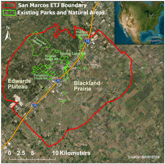
Figure 1.
Study area of San Marcos (Texas, USA) and its Extraterritorial Jurisdiction (ETJ). Important placenames mentioned in article are identified for reference, including the two ecoregions: Edwards Plateau (northwest of I-35) and Blackland Prairie (southeast of I-35).
2.2. Mapping Land Cover/Use and UGI from NAIP Imagery
2.2.1. Geospatial Data Sources
We used National Agriculture Imagery Program (NAIP) very-high-resolution (60 cm) aerial imagery from 2018 to classify land use for the San Marcos ETJ. The NAIP imagery used in this analysis had four bands: Blue (420–492 nm), Green (533–587 nm), Red (604–664 nm), and Near Infrared (683–920 nm), and was acquired at 4877 m (16,000 feet) above ground level (AGL) with a Leica ADS100 airborne digital sensor between May 2018 and April 2019 [119]. A total of 18 NAIP image tiles were necessary to cover the extent of the study area.
From the NAIP imagery, we calculated secondary datasets including Principal Components Analysis (PCA), Independent Component Analysis (ICA), the Normalized Difference Vegetation Index (NDVI), the Normalized Difference Water Index (NDWI), and the Soil Adjusted Vegetation Index (SAVI). We used vegetation and water indices to differentiate vegetation cover from non-vegetation cover. These indices also helped to distinguish between shadows and water bodies. From the PCA output, we calculated four texture measures including contrast, entropy, standard deviation, and dissimilarity. Finally, a Lidar dataset was downloaded from the USGS 3DEP program to address the topographical characteristics of the land cover classes. From the LiDAR dataset, we created a digital elevation model (DEM) as well as a canopy height model (CHM) at a 1 m spatial resolution. These additional datasets were used to help visually distinguish and mitigate uncertainty in land cover types during the training phase of the classification process.
2.2.2. Image Classification
Land cover classes of interest included the following eight land cover classes: trees, shrubs, grass, cropland, buildup area, water, barren/soil, and shadow. We digitized thirty signatures per land cover class for each of the 18 NAIP tiles separately. Prior to classification, 25% of the training polygons for each class were withheld to be used as validation data. The training data were used in three common classification algorithms: Random Forest (RF), Support Vector Machine (SVM), and Neural Network (NN). We performed the classifications separately for each NAIP tile using the ‘caret’ package in R version 4.2.0 [120,121]. Once the classifications were completed for each NAIP tile, we mosaicked the outputs for each classification algorithm into a single image file (e.g., RF mosaic and SVM mosaic). After the classification, we distinguished private and public land parcels using the parcel type attribute of the 2020 county appraisal district (CAD) geodatabase.
2.2.3. Accuracy Assessment
To assess the performance of the classification algorithms, we used the reserved training polygons to evaluate the agreement between the classified output and the reference data and created three separate accuracy assessment matrices, one for each classification algorithm. We used the accuracy assessment matrices to calculate the overall accuracy (OA), Kappa coefficient of agreement (K), and user (UA) and producer (PA) accuracy values for the overall map and each land cover class, respectively. Finally, to enhance the interpretability of the final classification map and mitigate “salt and pepper” effects [122], we applied a smoothing process using a majority filter with a 7 × 7 moving window [123].
2.3. Characteristics of Habitat Patches
The characteristics of land cover patches shape the connectivity and function of ecosystems [124,125]. We analyzed the land cover patches to assess the landscape’s characteristics before creating connectivity networks, utilizing common landscape metrics such as Core Area (CA), Landscape Shape Index (LSI), Proximity Index (PI), Area-Weighted Mean Shape Index (AWMSI), mean Patch Fractal Dimension (MPFD), and Shannon’s Evenness Index (SEI) [126,127]. Considering that habitat patches may experience human disturbances in urbanized areas, we used CA as a measure of habitat quality, indicating that a patch with higher CA is more suitable for the persistence of our chosen species. Our analysis also encompassed basic habitat patch statistics, including Total Area (TA), Mean Area (MA), Total Core Area (TCA), and Mean Core Area (MCA).
The CA integrates patch size, shape, and edge effect into a single measure. All else being equal, smaller patches with greater shape complexity have less core area. Most of the metrics associated with the size distribution (e.g., mean patch size and variability) can be formulated in terms of the core area. The Landscape Shape Index (LSI) reflects the complexity of patch shape. The Proximity Index (PI) quantifies the spatial context of a (habitat) patch in relation to its neighbors of the same class; it measures both the degree of patch isolation and the degree of fragmentation of the corresponding patch type within the specified neighborhood of the focal patch. The Area-Weighted Mean Shape Index (AWMSI) indicates the irregularity of shapes. A value of one suggests that all patches are circular (for polygons), and it increases with greater patch shape irregularity. The Mean Patch Fractal Dimension (MPFD) is another measure of shape complexity. The MPFD approaches a value of one for shapes with simple perimeters and approaches a value of two when shapes are more complex. Shannon’s Evenness Index (SEI) assesses the evenness or equitability of patch distribution. SEI ranges from 0 to 1, with 1 representing perfect evenness of patches and 0 indicating maximum inequality.
2.4. Networks and Corridor Identification
The first step of developing a UGI network is to identify the major nodes (i.e., large natural areas), followed by identifying potential corridors and ranking the networks. Using the least-cost path approach, we identified potential corridors in the San Marcos ETJ. The design of the path for UGI took into account the resistance/impedance value of the land use/land cover along the link. The efficiency depends on the source habitat and the resistance created by land uses along the path. The resistance also depends on the type of species. Our final product of potential corridors had multiple layers for each species. We designed the impedance for two species with different mobility and habitat requirements: (1) Golden-cheeked warbler (GCW, Setophaga chrysoparia), an endangered migratory bird species in the Texas Hill Country region whose primary mode of travel is in the air; and (2) Rio Grande wild turkey (RGWT, Meleagris gallopavo intermedia), a native year-round bird species whose primary mode of travel is on the ground.
To model habitat connectivity networks for San Marcos, Texas, we used the Golden-cheeked warbler (GCW) and Rio Grande wild turkey (RGWT) as focal species because of their ecological and cultural importance to the region, as well as their different mobility and habitat requirements. The federally endangered GCW inhabit oak mottes and mixed Ashe juniper and hardwood woodlands on canyons and ravines in the Edwards Plateau ecoregion, and they feed on insects and spiders found on the bark and leaves of these trees. This specialist species migrates to Central Texas from Mexico and Central America in March to nest and raise their young, returning to their winter home in July. Males are highly territorial of nest sites, and female GCWs only lay three to four eggs during the entire nesting season. Their habitats are vanishing from natural to non-natural land cover changes resulting from housing, roads, industry, and agriculture [128,129].
The RGWT is one of two remaining species of wild turkey native to North America and is the ancestor of the domestic turkey. RGWTs found in Texas sympatrically speciated from southeast Mexico. Wild turkeys are ground birds that occupy hardwood and mixed conifer–hardwood forests with scattered shrubs, fields, orchards, floodplains, and seasonal marshes. They prefer to live in dense native and mature plant communities where canopy openings are widely available [130]. RGWT habitats have also been declining due to urban and rural land cover changes [131,132].
We characterized the habitat/movement of the GCW and RGWT using published literature and expert consultation. We used a comprehensive matrix of land-cover resistance in determining the connectivity of habitat patches for the two separate species. There is no established resistance value for land cover features for species movement [133,134], therefore we used values based on ad hoc data following the studies that modeled connectivity between forest habitat patches [135,136,137,138]. We consulted with six experts from the Texas A&M AgriLife Extension Service and the Texas Parks and Wildlife Department (TPWD) who specialize in GCW and RGWT. We collected the resistance scores they assigned for specific land cover types, derived relative scores, and consulted with them again to finalize the resistance values.
Using the sources above, we assigned path resistance values that took into account habitat size, land use type, and road networks along the path [139,140]. These resistance values (1 to 1000) are theoretical variables that represent relative estimates of the resistance to movement through the path. We calculated resistance values using the Rating and Weighting (RAW) method [141], the Delphi method [142], and insights from previous transportation studies [143]. We assigned a value of 1 to a land use with no resistance, while the land use with the highest resistance received a maximum impedance of 1000 (Table 1 and Table 2). For both species, artificial structures such as buildings and roads had the highest resistance values, but most resistance values were proportionally higher for RGWT (Table 2) compared to GCW (Table 1) because RGWT primarily moves along the ground while GCW moves aerially. The resulting weighted land cover maps were transformed into a habitat suitability map for use as a cost surface in the least-cost path analysis.

Table 1.
Resistance value classes for Golden-cheeked warbler (GCW).
Table 2.
Resistance value classes for Rio Grande wild turkey (RGWT).
2.5. Priority Networks for Indicator Species
We mapped and examined the distribution of specific habitat patches/corridors and the best potential networks to connect them. In general, areas (or patches) have a greater interaction when they are larger and closer together [139]. Patch weight is necessary to apply the gravity model. We assigned a weight to each patch based on the size and habitat preferences by species. We used GCW and RGWT survey data from previous studies supported by SMGA (San Marcos Greenbelt Alliance), USFWS (U.S. Fish and Wildlife Service), TXST (Texas State University), and CoSM (The City of San Marcos) to assign weights. Weights determine the relative significance with reference to the habitat requirement [139].
where Na is the patch weight for the GCW and RGWT habitat patch, Xa is the area of the patch, and Sa is the minimum area required for the indicator species. Weight was multiplied by 10 to normalize the value. We used the following equation to inform the gravity model (Gab):
where Gab is the level of interaction between patches a and b, Na is the weight of patch a, Nb is the weight of patch b, and Dab is the distance between centroids of patches a and b. The gravity model determined different levels of interactions between patches. We used the patch center over the patch edge for our bird species as the center of a patch is less influenced by irregularities in patch shape and edge effects. We used the Python programming language to estimate and evaluate multiple potential networks and identified the most effective models through a Monte Carlo simulation. We conducted 550 iterations in the simulation process to attain a 95% confidence level. The importance and significance of these networks can be identified using the Gamma and Beta indices. The Gamma ratio represents the percentage of connectivity within each network. The Beta index indicates the complexity of the network; it is calculated by dividing the number of links by the number of patches.
We used graph theory to represent the habitat patches as a series of interconnected patches, where flows occurred as a result of structural and/or functional patch connectivity [144]. We analyzed several graph components for each of the selected networks. These were the evenness index [145], core area index [146], shape complexity [147], and edge density of patches [148]. These indices provided a quantitative description of GCW and RGWT habitat structures.
After constructing habitat networks and ranking networks using gravity models, we analyzed the share of semi-natural areas that occurred on private lands. To understand the contributions of neighborhood lands on proposed networks, we used San Marcos Council of Neighborhood Associations (CONA)-defined boundaries along with census tracts. These boundaries comparatively reflected the basic characteristics of a coherent physical layout, shared infrastructure, common land uses, and a sense of community.
3. Results
3.1. Land Cover Distributions
The 0.6-m resolution land cover map we produced for the city of San Marcos achieved an overall accuracy of 88% using the Random Forest (RF) algorithm, with a Kappa coefficient of 0.85 (Table A1 in Appendix A). We did not use the Support Vector Machine (SVM) and Neural Network (NN) algorithms because of their overall lower accuracies of 85% and 82%, respectively. Our land cover map revealed several major patterns (Figure 2). The northwestern half of the study area had relatively high forest and shrub cover (62%), characteristic of the Edwards Plateau ecoregion. Single-family residential neighborhoods and adjacent parks in this ecoregion had the densest forest cover, while most of the large ranches had savanna landscapes that were mostly grassland with small patches of shrubs/trees. The southeastern half of the study area was dominated by grasslands and cropland (>75%), characteristic of the Blackland Prairie ecoregion. Most of the trees in this ecoregion followed river networks. There were also a lot of trees around the central historic district of San Marcos. Aside from downtown San Marcos, most of the urban development followed the Interstate 35 corridor that approximately marks the dividing line between the two ecoregions. Developed land cover (7.6%) was higher in the Blackland Prairie region than in the Edwards Plateau region (5.1%) (Table 3).
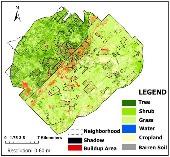
Figure 2.
Final land cover map of San Marcos ETJ applying Random Forest (RF) classification algorithm (Image: NAIP, Resolution: 0.6 m).
Table 3.
Land cover distribution in San Marcos ETJ.
Semi-natural areas (trees, shrubs, and grass) covered 371 km2 (or 74%) of the entire study area (Table 3). Most of these semi-natural areas (59%) occurred on private land, with 15% occurring in residential neighborhoods and 44% occurring on other private land like ranches. The share of tree, shrub, and grass cover within neighborhood boundaries was slightly higher than the whole ETJ pattern, with percentages of 16.2%, 20.3%, and 43.5%, respectively. The tree and shrub cover in privately owned parcels exhibited slightly lower percentages than the overall pattern, with 12.1% and 15.4%, respectively. In contrast, the grass share saw a slight increase, rising from 42.4% in whole ETJ to 45.5% in private lands (Table 3).
3.2. Spatial Patterns of Habitat Patches
Using the land cover map in Figure 2, we selected common landscape metrics to quantify spatial patch characteristics, patch classes, and landscape mosaics. Given that small UGI patches cannot support GCW, we selected UGI patches larger than 0.1 km2, the minimum habitat requirement for GCW [149]. Our second indicator species, RGWT, can be found in grassland and cropland along with trees [150]. For the RGWT habitat, we extracted cropland, grass, and tree cover larger than 0.01 km2. We identified a total of 107 UGI patches with an area larger than 0.1 km2 as GCW habitats, which account for 85% of the total vegetation cover and 33% of the whole study area. RGWT habitats consisted of 1874 patches, which is approximately 49% of the study area.
Regarding landscape metrics, the mean patch size and mean core area were significantly higher for GCW than RGWT because the threshold value for GCW was higher than for RGWT (Table 4). The AWMSI value for the GCW habitat area was 66.66, signifying highly irregular shapes. A value of 1 represents a regular shape, while higher values (≥1) indicate more irregular shapes. The habitat shape for RGWT showed less irregularity (AWMSI = 40.11) than the GCW habitat. The Mean Patch Fractal Dimension (MPFD) assesses the shape complexity. An MPFD of 1 indicates simple perimeters, while a value of 2 indicates more complex perimeters. The MPFD values of 1.57 (GCW) and 1.4 (RGWT) indicated that both habitats were complex in shape (Table 4). Shannon’s Evenness Index (SEI), which measures the evenness of patches, indicated a medium level of evenness for GCW habitats (0.53) and a more even distribution for RGWT (0.62). These patch indices are important for understanding the spatial characteristics of habitat quality, which influence the connectivity of UGI patches. For example, higher mean patch size and core area for GCW suggest more substantial and potentially more viable habitats, while irregular shapes and complex perimeters diminish the ease of movement and connectivity for species.
Table 4.
Landscape metrics of patches suitable for Golden-cheeked Warbler (GCW) and Rio Grande Wild Turkey (RGWT) in San Marcos ETJ.
3.3. UGI Networks for Golden-Cheeked Warbler (GCW) and Priority Areas
We extracted UGI networks for GCW by applying a gravity model and graph theory to connect the major habitat patches. The outcome found that the northwest region of San Marcos featured a concentrated core area of habitat patches, functioning as a vital hub within the study area and potentially offering essential resources and habitat for GCW (Figure 3). The corridors formed the arteries of the networks and correspond to vegetated areas along riparian zones, private green spaces, and roadside green infrastructure. Dense forests predominantly covered these corridors, occasionally interrupted by openings created by agricultural fields or other land covers.
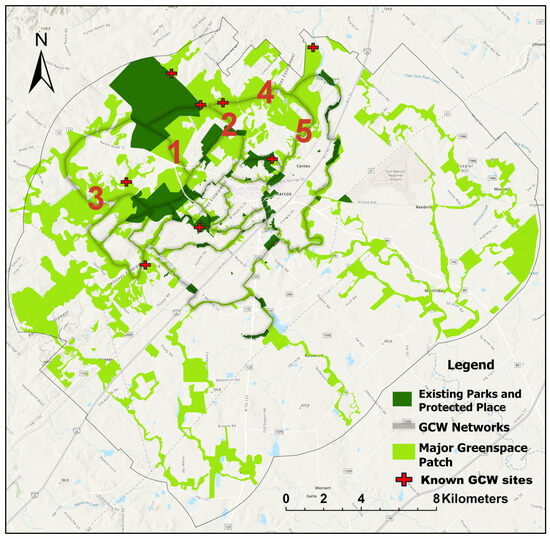
Figure 3.
Potential connected habitat networks for Golden-cheeked Warbler (GCW) in San Marcos ETJ, with suitability ranking (red number) located in the middle of the linear corridor. Major greenspace patches were identified using a threshold patch area of 0.10 km2.
The modeled GCW networks, which encompassed 93.43% of semi-natural vegetation cover (tree, shrub, and grass), 3.79% of croplands, and 1.75% of buildup areas, collectively covered 32.87% of the study area (Table 5). Analyzing the distribution of each land cover type, we found that 80.5% of the tree cover and 78.3% of the shrub cover were integrated into the ecological networks (Table 5). Buildings and roads were major barriers to connectivity. The network for GCW avoided buildup areas because of the high impedance value. However, buildup areas, water, and barren soil also contributed to the formation of networks in areas where low-resistance land cover was not available (Figure 3).
Table 5.
Distribution of potential habitat networks for Golden-Cheeked Warbler (GCW).
In Table 5, the GCW networks on private lands and neighborhood lands are separately outlined. This clear separation allows for a detailed analysis of the network’s land cover patterns, both on private properties and within the defined neighborhood areas. Table 5 shows that 58.19% of GCW networks were established on privately owned land parcels, while 22.17% were within neighborhood areas. The majority of these networks were established using grass, shrubs, and tree cover on private lands.
We ranked corridors for each alternative network through an analysis of existing habitat survey data and the interactions between patches using graph theory and gravity model as described in Section 2.5. We calculated the degree of interaction based on patch size and distance between patches. The potential corridor primarily ran through an area with the largest high-quality habitat patches in the northwest (Figure 3). Corridors with high rankings (i.e., 1, 2, 3, 4, and 5) showed high degrees of connectivity through tree patches in neighborhood areas (Figure 3, marked in red). This ranking system served as a guide for prioritizing habitat networks for GCW. The first-ranked corridor for GCW traversed through Ranch Road 12 and a neighborhood called West Centerpoint connecting Freeman Ranch and Purgatory Creek Natural Area, two major GCW habitat areas. The second-ranked corridor connected Ringtail Ridge Natural Area and other adjacent natural areas to Freeman Ranch, linking through the Country/Backus Estates neighborhood. The third-ranked corridor for GCW ran through the pathway of Purgatory Creek and Sink Creek, connecting Purgatory Creek natural areas to Freeman Ranch. The fourth- and fifth-ranked corridors connected Five Mile Dam Park and San Marcos River parks to Freeman Ranch, traversing through neighborhoods and green areas to the north.
Neighborhood green spaces surrounding existing natural areas acted as the main connector to the source, accounting for 9% of the overall networks (Figure 3). There were also corridors in the northeast and southeast that followed the San Marcos River. Networks for GCW were not functional in these areas because of the isolation from main habitat sources. GCW mainly inhabited the northwest side (Edwards Plateau) of the study area (Figure 3). The most significant habitat impedance appeared along Interstate 35 and the southeast side of the study area, where road networks, spreading development, and large croplands dominated (Figure 3).
3.4. UGI Networks for Rio Grande Wild Turkey (RGWT) and Priority Areas
The UGI networks for RGWT were comparatively dispersed because of their habitat characteristics (Figure 4). Habitat areas for RGWT included trees, grasses, and cropland patches greater than 10,000 m2. The core areas for RGWT habitats were located in the northeast and northwest areas. The patches in the other core areas were distributed in linear patterns, mostly along stream networks.
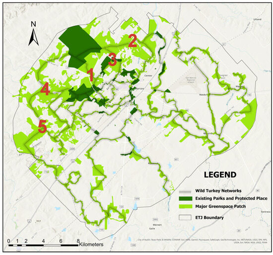
Figure 4.
Potential connected habitat networks Rio Grande Wild Turkey (RGWT) in San Marcos ETJ, with suitability ranking (red number) located in the middle of the linear corridor. Major greenspace patches were identified using a threshold patch area of 0.10 km2.
The RGWT networks comprised 88% vegetation cover (trees, shrubs, and grass), 11.6% croplands, and 0.5% buildup areas (Table 6). These networks collectively encompassed nearly half of the study area. High resistance along the pathways led to the inclusion of buildup areas, water bodies, and barren soil in less than 1% of these networks. These acted as significant obstacles to connectivity, likely isolating habitat patches for RGWT. Private semi-natural lands significantly contributed to the proposed RGWT networks. Approximately 62.41% of RGWT networks were located within private lands, and 23% of these were within single-family neighborhoods that contributed to these networks.
Table 6.
Structural analysis of the potential habitat network for Rio Grande Wild Turkey (RGWT).
The priority networks for RGWT were in the northwest and southeast areas, connecting core areas of habitat patches (Figure 4). The first-ranked corridor connected the two largest protected areas in the city’s ETJ, Purgatory Creek Natural Area and Freeman Ranch. The second-ranked corridor extended from Freeman Ranch to other large ranches and a low-density neighborhood. The third-priority corridor stretched from the Spring Lake Natural Area (north of downtown San Marcos) to Freeman Ranch (northwest of downtown San Marcos) via Sink Creek and the Country/Backus Estates neighborhood. The fourth-priority corridor linked two significant source layers, Purgatory Creek Natural Area and Freeman Ranch, through Purgatory Creek to the west. The fifth-priority corridor connected major patches located in the southwest, specifically those along York Creek and Purgatory Creek. Corridors along Interstate 35 were poorly connected, especially close to the city center because of the high impedance value of roads and buildings. Unlike GCW habitats, there were networks along the Blackland Prairie ecoregion; however, because of the habitat characteristics, these networks ranked lower compared to the Edwards Plateau (Figure 4).
4. Discussion
4.1. UGI Connectivity: Graph Theory and Gravity Model
The objective of this study was to map and analyze urban green infrastructure (UGI) networks for two species with a specific emphasis on the contribution of mostly small private semi-natural areas to the connectivity of these networks. To fulfill the research goal, our study employed a combination of landscape metrics, graph theory, the gravity model, and least-cost path analyses. This multi-method approach presents new opportunities for land conservation and ecological restoration. We believe that our methodology of using path impedance to identify potential habitat corridors for GCW and RGWT is a more accurate approximation of UGI connectivity compared to randomly selected linkage approaches [151,152].
The use of the gravity model added a useful layer of network preference for selected species. The determination of the relative significance of each green space within the network offered valuable guidance for improved UGI planning. The gravity model considers the size and proximity of UGI, which more accurately models how species move through urban environments [153]. Previous studies found the gravity model to be particularly useful in fragmented landscapes [138,153,154]. Similarly, the utilization of least-cost path analysis to identify potential corridors resulted in a realistic representation of the complex landscape, which is critical for successful conservation and urban planning efforts [139,155,156,157].
In fragmented urban landscapes, the complexity of UGI poses challenges in assessing the value of planned networks, particularly in terms of connectivity [158,159]. Fischer and Lindenmayer [160] explained that evaluating these networks requires considering various factors such as spatial configuration, ecological processes, and the integration of multiple green spaces to ensure effective connectivity and functionality. Li et al. [161] recommend future studies to adopt a land use or land cover perspective, aligning with practical planning and design scales. The approach outlined in this study effectively identifies potential habitat corridors and patches as functional network components from a land-use/land cover (LULC) perspective.
4.2. Network Analysis for Indicator Species: Evaluating and Ranking Connectivity
Habitat networks for GCW and RGWT utilized 80% of the city’s total tree cover and almost 80% of the city’s shrublands (Table 5 and Table 6), revealing the importance of trees and shrubs (many of these young trees) for bird habitats in urban landscapes. Regarding land cover classes along the paths, we found that 37% consisted of trees, 41% of shrub cover, and 15.38% of grass for GCW. The land cover classes along the RGWT paths significantly changed, with 7.7% of the networks formed by cropland, 26.49% by trees, 34.04% by shrubs, and 31.44% formed by grass. Network land cover distributions showed that over 90% formed with vegetation cover (trees, shrubs, and grass) with little inclusion of other land cover types like barren land, cropland, and buildup areas. The contribution of vegetation in proposed lands proved that San Marcos ETJ has an abundance of vegetation cover, and proper utilization of these vegetated areas could lead to a rich biodiversity network.
Looking at the spatial distribution of the proposed networks, the northwestern region of San Marcos, known as the Edwards Plateau ecoregion, exhibited high tree cover density and minimal urban development, making it an ideal habitat for both the GCW and RGWT populations. Existing large parks and natural areas also made it a suitable place for GCW and RGWT habitats. Although GCW networks were mainly concentrated in the northwestern area, RGWT networks had the potential to grow and expand through the southeastern part of the ETJ (Figure 4).
In a comparable study, Lopes, et al. [162] analyzed greenway networks in urbanized areas where the share of impervious land cover was higher than the pervious cover and found that networks were mainly concentrated in peripheral areas near the existing natural source areas. While there was a relatively high concentration of favorable habitat patches distributed throughout our study area (at least the Edwards Plateau half of the city; Figure 3 and Figure 4), they were not contiguous or connected, potentially creating challenges for wildlife movement. Thus, priority corridors play a crucial role in structurally and functionally connecting these UGI patches. This approach aligns with the study conducted by Huang et al. [163], which demonstrated that planned ecological networks enhance the shape complexity of green patches, improve landscape connectivity, and reduce fragmentation.
In our study area, the first-priority corridor for both the GCW (Figure 3) and RGWT (Figure 4) is a perfect example of how one parcel of land (location of the red 1) is key to the movement of wildlife from one large, protected area to another. In San Marcos, this parcel connected the 14.1 km2 protected Freeman Ranch with the 2.83 km2 Purgatory Creek Natural Area and its extended network of trails and natural areas. Unfortunately, this land parcel was targeted for development in 2023, threatening the major wildlife corridor in San Marcos [164].
We assessed potential network configurations by overlaying land-use patterns and habitat preferences of two indicator species. This approach allowed us to create networks in a complex urban landscape and identify potential challenges that may arise during network construction. Jongman [165] stated that creating connected green space networks is a complex process and should not be based on species distribution data but rather follow a more comprehensive long-term strategy. To address this complexity, researchers recommend site-specific, multi-scale modeling with consideration of structural and functional connectivity [86,165,166], as we did in this study.
4.3. UGI Connectivity: The Role of Private Semi-Natural Lands
Numerous studies have documented semi-natural habitat loss due to urbanization and agriculture [167,168,169,170]. In addition to reducing overall habitat areas, these processes decreased the connectivity of the remaining fragments [171,172]. To successfully restore semi-natural habitats, Harlio et al. [173] emphasized the importance of both site restoration and prioritizing the improvement of habitat connectivity. Hooftman and Bullock [106] suggested that this process begins with detailed mapping of long-term habitat changes on a fine scale, providing baseline information about past habitat configurations. Lindenmayer et al. [174] focused on understanding the cumulative impacts of landscape processes and improving connectivity strategies to balance ecological benefits. Other previous research directed restoration efforts to focus on creating ecological networks that are easy to restore and have more ecological value [175,176,177]. Paloniemi and Tikka [107] investigated how different stakeholders perceive the habitat connectivity process. They highlighted the necessity for a ‘multilateral governance approach’ to integrate privately owned semi-natural lands into the broader ecosystem, aiming to enhance overall biodiversity.
Our analysis found a significant role of private semi-natural green space in the overall UGI networks. The priority habitat corridors we identified covered 124 km2 for GCW and 252.9 km2 for RGWT. Within the 124 km2 of GCW habitats, a total of 71.92 km2 spanned through privately owned land parcels, making up approximately 59% of the entire GCW habitat networks. Within the extensive habitat network spanning 252.9 km2 for RGWT, a total of 155 km2 (61.2%) were connected through privately owned ranches, farms, and individual land parcels. This intricate interconnection highlights the integration of these vital private ranches and farms within broader biodiversity conservation networks.
Texas working lands encompassing farms, ranches, and forests play a vital role in food production, supporting rural economies and providing diverse benefits [178]. Between 1997 and 2017, Texas saw the transformation of about 8900 km2 of designated working lands into non-agricultural uses [178]. A significant portion of this area, nearly 485 km2, occurred in the last five years of that period. Historically, farms and ranches have given way to urban areas, but the current pace of land conversion is unprecedented, driven by increasing incentives for landowners to sell or subdivide. This swift shift in land use jeopardizes the region’s cultural and natural heritage resources [179,180]. Preserving these ranches and farms and their benefits is a significant challenge, highlighting the urgent need for sustainable conservation strategies in the face of relentless development pressure. Conservation efforts, reliant on private landowners through methods like conservation easements, are challenged by limited protected areas and conservation alternatives. Farms and ranches played a vital role in proposed GCW and RGWT networks, highlighting the importance of including these lands in biodiversity conservation efforts through conservation easements.
A substantial section of both GCW and RGWT networks was located within the boundaries defined by the Council of San Marcos Neighborhood Association (CONA). For instance, 15 km2 of GCW networks, equivalent to 22.17% of the total GCW networks, passed through neighborhood areas. In the case of RGWT, approximately 35.93 km2 of networks, nearly 23% of the overall RGWT networks, traversed through neighborhoods. These findings suggest that a substantial portion of semi-natural areas in neighborhoods such as yards, gardens, parks, easements, and greenspaces could contribute to connecting the existing parks and protected places.
Our study illustrated that private green spaces within the San Marcos ETJ play a significant role in UGI and enhance habitats for birds and wildlife [181,182]. To further leverage these benefits, the next step should be to preserve accessibility to these lands and integrate them into the broader ecological system. Conservation easements could ensure this accessibility. Hayward and Kerley [183] highlighted how the simple easement approach caused substantial changes in urban neighborhood ecosystems. Rudd, Vala, and Schaefer [157] explained the role of backyards in biodiversity conservation and criticized the role of government bodies for the failure to adopt simple wildlife conservation strategies. The City of San Marcos is engaged in the Edwards Aquifer Habitat Conservation Plan (EAHCP), primarily focusing on river-based ecosystems and existing protected areas. However, upon reviewing the 2019 San Marcos Parks, Recreation, and Open Space Master Plan, it is evident that there is no emphasis on conservation easements or community involvement for biodiversity conservation in privately owned lands. Our findings suggest that private green spaces could play a similar role for wildlife movement (Figure 2, Figure 3 and Figure 4) as those in wildlands. It becomes apparent that relatively small interventions such as implementing fence-free easements and constructing minimal green corridors could facilitate the movement of birds and wildlife. These deed restriction practices exist in some San Marcos neighborhoods but have not been strictly enforced, a problem found in other communities as well [184].
Higher-level government policies could also enhance ecological corridors in private and residential areas [185]. Two examples are incentivized tree-planting programs and wildlife tax exemptions—a property tax incentive program designed to encourage landowners to manage a portion of their property for wildlife habitat. Current wildlife tax exemptions in Texas require a minimum of 14–20 acres of land [186]. This law restricts the integration of medium and small-sized parcels into the broader UGI network. While large natural areas are most desirable, a connected network of semi-natural blue–green spaces have significant conservation value [187]. Moving forward, land conservation strategies should include (1) changes in local and state tax policies to broaden wildlife tax exemptions to smaller lands and (2) community-based conservation initiatives where neighboring landowners collaborate to create wildlife corridors and shared conservation areas [185,188,189].
5. Conclusions
In the context of rapid urbanization and landscape fragmentation, this study mapped and analyzed urban green-–blue infrastructure (UGI) networks, with a particular focus on the role played by private semi-natural landscapes. Private semi-natural green spaces in our case study were indeed important for ecological habitat, with 60% of the priority habitat corridors traversing through private parcels and 23% through neighborhood areas. Riparian zones and other concentrations of trees stood out as key corridor linkages. Our findings reaffirm the importance of integrating private green spaces, even small ones, into urban wildlife habitat plans.
Our study focused on bird habitats and corridors; however, UGI connectivity also aids humans by establishing a network of accessible and functional green spaces that provide ecosystem services and other needs of residents/visitors [190,191]. Understanding the relationship between social movement and UGI is important for holistic health approaches [192], and future studies should assess UGI within the context of social–ecological systems. There is also evidence that improving access to nature benefits social cohesion and community well-being [193].
Author Contributions
Conceptualization, R.J. and J.P.J.; methodology, R.J., J.P.J., J.L.R.J., and K.M.M.; software, R.J.; validation, R.J.; formal analysis, R.J.; investigation, R.J.; resources, R.J. and J.L.R.J.; data curation, R.J.; writing—original draft preparation, R.J. and J.P.J.; writing—review and editing, R.J., J.P.J., J.L.R.J., and K.M.M.; visualization, R.J.; supervision, J.P.J., J.L.R.J., and K.M.M.; project administration, J.P.J.; funding acquisition, R.J. All authors have read and agreed to the published version of the manuscript.
Funding
This research was funded by a student research fellowship (2020-0091) to Raihan Jamil from the San Marcos Greenbelt Alliance (SMGA). SMGA is a nonprofit organization working to protect the quality of life for the people of San Marcos through the creation of interconnected parks and natural areas. The content and views expressed in this article are solely the responsibility of the authors and do not necessarily represent the official views of, nor an endorsement of, the funder.
Data Availability Statement
The data presented in this study are available upon request from the corresponding author.
Acknowledgments
Several individuals assisted with our methodology and provided data, including Rebekah Rylander (Rio Grande Joint Venture), Sherwood Bishop (SMGA), Ashley Long (Texas A&M Institute of Renewable Natural Resources), William P. Kuvlesky Jr. (Texas A&M University–Kingsville), and Derrick Wolter (TPWD).
Conflicts of Interest
The authors declare no conflicts of interest. The funders had no role in the design of the study; in the collection, analyses, or interpretation of data; in the writing of the manuscript; or in the decision to publish the results.
Appendix A
Table A1.
Land cover confusion matrix to estimate the Random Forest (RF) classification accuracy.
Table A1.
Land cover confusion matrix to estimate the Random Forest (RF) classification accuracy.
| Reference data | ||||||||||
| Land cover type | Water | Buildup | Shadow | Barren Soil | Cropland | Grass | Shrub | Tree | User accuracy | |
| Classification data | Water | 8 | 0 | 0 | 0 | 0 | 0 | 0 | 0 | 1.00 |
| Buildup | 0 | 10 | 0 | 0 | 0 | 0 | 0 | 0 | 1.00 | |
| Shadow | 1 | 0 | 7 | 0 | 0 | 0 | 0 | 0 | 0.88 | |
| Barren | 0 | 0 | 0 | 9 | 0 | 1 | 0 | 0 | 0.90 | |
| Cropland | 0 | 0 | 0 | 1 | 18 | 3 | 0 | 0 | 0.82 | |
| Grass | 0 | 0 | 0 | 1 | 4 | 22 | 1 | 0 | 0.79 | |
| Shrub | 0 | 0 | 0 | 0 | 0 | 1 | 22 | 2 | 0.88 | |
| Trees | 0 | 0 | 0 | 0 | 0 | 0 | 1 | 21 | 0.95 | |
| Producer accuracy | 0.89 | 1.00 | 1.00 | 0.82 | 0.82 | 0.81 | 0.92 | 0.91 | ||
| Overall accuracy | 0.88 | |||||||||
| Kappa | 0.85 | |||||||||
References
- Mitchell, M.G.; Devisscher, T. Strong relationships between urbanization, landscape structure, and ecosystem service multifunctionality in urban forest fragments. Landsc. Urban Plan. 2022, 228, 104548. [Google Scholar] [CrossRef]
- Dobbs, C.; Kendal, D.; Nitschke, C.R. Multiple ecosystem services and disservices of the urban forest establishing their connections with landscape structure and sociodemographics. Ecol. Indic. 2014, 43, 44–55. [Google Scholar] [CrossRef]
- Weng, Q.; Lu, D. Landscape as a continuum: An examination of the urban landscape structures and dynamics of Indianapolis City, 1991–2000, by using satellite images. Int. J. Remote Sens. 2009, 30, 2547–2577. [Google Scholar] [CrossRef]
- Ode, Å.; Fry, G.J.L. A model for quantifying and predicting urban pressure on woodland. Landsc. Urban Plan. 2006, 77, 17–27. [Google Scholar] [CrossRef]
- Haddad, N.M.; Brudvig, L.A.; Clobert, J.; Davies, K.F.; Gonzalez, A.; Holt, R.D.; Lovejoy, T.E.; Sexton, J.O.; Austin, M.P.; Collins, C.D. Habitat fragmentation and its lasting impact on Earth’s ecosystems. Sci. Adv. 2015, 1, e1500052. [Google Scholar] [CrossRef]
- Di Giulio, M.; Holderegger, R.; Tobias, S. Effects of habitat and landscape fragmentation on humans and biodiversity in densely populated landscapes. J. Environ. Manag. 2009, 90, 2959–2968. [Google Scholar] [CrossRef] [PubMed]
- Cousins, S.A.; Ohlson, H.; Eriksson, O. Effects of historical and present fragmentation on plant species diversity in semi-natural grasslands in Swedish rural landscapes. Landsc. Ecol. 2007, 22, 723–730. [Google Scholar] [CrossRef]
- Brückmann, S.V.; Krauss, J.; Steffan-Dewenter, I. Butterfly and plant specialists suffer from reduced connectivity in fragmented landscapes. J. Appl. Ecol. 2010, 47, 799–809. [Google Scholar] [CrossRef]
- Helman, A.; Zarzo Arias, A.; Penteriani, V. Understanding potential responses of large carnivore to climate change. Hystrix 2022, 32. [Google Scholar] [CrossRef]
- Fischer, J.; Lindenmayer, D.B. Landscape modification and habitat fragmentation: A synthesis. Glob. Ecol. Biogeogr. 2007, 16, 265–280. [Google Scholar] [CrossRef]
- Collinge, S.K. Ecological consequences of habitat fragmentation: Implications for landscape architecture and planning. Landsc. Urban Plan. 1996, 36, 59–77. [Google Scholar] [CrossRef]
- Timmermans, W. Ecological models and urban wildlife. WIT Trans. Ecol. Environ. 1970, 46, 12. [Google Scholar]
- Opdam, P.; Steingröver, E.; Van Rooij, S. Ecological networks: A spatial concept for multi-actor planning of sustainable landscapes. Landsc. Urban Plan. 2006, 75, 322–332. [Google Scholar] [CrossRef]
- Bascompte, J. Structure and dynamics of ecological networks. Science 2010, 329, 765–766. [Google Scholar] [CrossRef] [PubMed]
- Mukherjee, M.; Takara, K. Urban green space as a countermeasure to increasing urban risk and the UGS-3CC resilience framework. Int. J. Disaster Risk Reduct. 2018, 28, 854–861. [Google Scholar] [CrossRef]
- Pickett, S.T.; Cadenasso, M.L.; Grove, J.M.; Nilon, C.H.; Pouyat, R.V.; Zipperer, W.C.; Costanza, R. Urban ecological systems: Linking terrestrial ecological, physical, and socioeconomic components of metropolitan areas. Annu. Rev. Ecol. Syst. 2001, 32, 127–157. [Google Scholar] [CrossRef]
- Madureira, H.; Andresen, T.; Monteiro, A. Green structure and planning evolution in Porto. Urban For. Urban Green. 2011, 10, 141–149. [Google Scholar] [CrossRef]
- Van Oijstaeijen, W.; Van Passel, S.; Cools, J. Urban green infrastructure: A review on valuation toolkits from an urban planning perspective. J. Environ. Manag. 2020, 267, 110603. [Google Scholar] [CrossRef] [PubMed]
- Cook, E.A.; Van Lier, H.N. Landscape planning and ecological networks. In Landscape Planning and Ecological Networks; Elsevier, Developments in Landscape Management & Urban Planning, 6F: Amsterdam, The Netherlands, 1994. [Google Scholar]
- Gill, S.E.; Handley, J.F.; Ennos, A.R.; Pauleit, S. Adapting cities for climate change: The role of the green infrastructure. Built Environ. 2007, 33, 115–133. [Google Scholar] [CrossRef]
- Jennings, V.; Baptiste, A.K.; Osborne Jelks, N.T.; Skeete, R. Urban green space and the pursuit of health equity in parts of the United States. Int. J. Environ. Res. Public Health 2017, 14, 1432. [Google Scholar] [CrossRef]
- So, S.W. Urban Green Space Accessibility and Environmental Justice: A Gis-Based Analysis in the City of Phoenix, Arizona. Master’s Thesis, University of Southern California, Los Angeles, CA, USA, 2016. [Google Scholar]
- Jennings, V.; Bamkole, O. The relationship between social cohesion and urban green space: An avenue for health promotion. Int. J. Environ. Res. Public Health 2019, 16, 452. [Google Scholar] [CrossRef]
- Horwood, K. Green infrastructure: Reconciling urban green space and regional economic development: Lessons learnt from experience in England’s north-west region. Local Environ. 2011, 16, 963–975. [Google Scholar] [CrossRef]
- Gulsrud, N.M.; Ostoić, S.K.; Faehnle, M.; Maric, B.; Paloniemi, R.; Pearlmutter, D.; Simson, A.J. Challenges to Governing Urban Green Infrastructure in Europe–The Case of the European Green Capital Award. In The Urban Forest: Cultivating Green Infrastructure for People and the Environment; Springer: Cham, Switzerland, 2017; pp. 235–258. [Google Scholar]
- Wilkes-Allemann, J.; Kopp, M.; Van der Velde, R.; Bernasconi, A.; Karaca, E.; Čepić, S.; Tomićević-Dubljević, J.; Bauer, N.; Petit-Boix, A.; Brantschen, E.C. Envisioning the future—Creating sustainable, healthy and resilient BioCities. Urban For. Urban Green. 2023, 84, 127935. [Google Scholar] [CrossRef]
- Benedict, M.A.; McMahon, E.T. Green infrastructure: Smart conservation for the 21st century. Renew. Resour. J. 2002, 20, 12–17. [Google Scholar]
- Beatley, T.; Manning, K. The Ecology of Place: Planning for Environment, Economy, and Community; Island Press: Washington, DC, USA, 1997; p. 132. [Google Scholar]
- Flores, A.; Pickett, S.T.; Zipperer, W.C.; Pouyat, R.V.; Pirani, R. Adopting a modern ecological view of the metropolitan landscape: The case of a greenspace system for the New York City region. Landsc. Urban Plan. 1998, 39, 295–308. [Google Scholar] [CrossRef]
- Cui, L.; Wang, J.; Sun, L.; Lv, C. Construction and optimization of green space ecological networks in urban fringe areas: A case study with the urban fringe area of Tongzhou district in Beijing. J. Clean. Prod. 2020, 276, 124266. [Google Scholar] [CrossRef]
- Luque, S.; Saura, S.; Fortin, M.-J. Landscape connectivity analysis for conservation: Insights from combining new methods with ecological and genetic data. Landsc. Ecol. 2012, 27, 153–157. [Google Scholar] [CrossRef]
- Merriam, G. Connectivity: A fundamental ecological characteristic of landscape pattern. In Proceedings of the Methodology in Landscape Ecological Research and Planning: Proceedings, 1st Seminar, International Association of Landscape Ecology, Roskilde, Denmark, 15–19 October 1984. [Google Scholar]
- Levins, R. Some demographic and genetic consequences of environmental heterogeneity for biological control. Bull. ESA 1969, 15, 237–240. [Google Scholar] [CrossRef]
- Den Boer, P.J. Spreading of risk and stabilization of animal numbers. Acta Biotheor. 1968, 18, 165–194. [Google Scholar] [CrossRef]
- Adriaensen, F.; Chardon, J.; De Blust, G.; Swinnen, E.; Villalba, S.; Gulinck, H.; Matthysen, E. The application of ‘least-cost’modelling as a functional landscape model. Landsc. Urban Plan. 2003, 64, 233–247. [Google Scholar] [CrossRef]
- Philip, D.T.; Fahrig, L.; Henein, K.; Merriam, G.J.O. Connectivity is a vital element of landscape structure. Oikos 1993, 68, 571–573. [Google Scholar]
- Philip, D.T.; Fahrig, L.; With, K.A. Landscape connectivity: A return to the basics. In Connectivity Conservation; Conservation Biology Series; Cambridge University Press: Cambridge, UK, 2006; Volume 14, pp. 29–43. [Google Scholar]
- Lindenmayer, D.; Fischer, J. Landscape Change and Habitat Fragmentation: An Ecological and Conservation Synthesis; Island Press: Washington, DC, USA, 2006; pp. 51–59. [Google Scholar]
- Bodin, Ö.; Saura, S. Ranking individual habitat patches as connectivity providers: Integrating network analysis and patch removal experiments. Ecol. Model. 2010, 221, 2393–2405. [Google Scholar] [CrossRef]
- Rodrıguez, A.; Delibes, M.J.B.c. Population fragmentation and extinction in the Iberian lynx. Biol. Conserv. 2003, 109, 321–331. [Google Scholar] [CrossRef]
- Brook, B.W.; Tonkyn, D.W.; O’Grady, J.J.; Frankham, R. Contribution of inbreeding to extinction risk in threatened species. Conserv. Ecol. 2002, 6, 16. [Google Scholar] [CrossRef]
- Hanski, I. Habitat connectivity, habitat continuity, and metapopulations in dynamic landscapes. Oikos 1999, 87, 209–219. [Google Scholar] [CrossRef]
- Pimm, S.L.; Diamond, J.; Reed, T.M.; Russell, G.J.; Verner, J. Times to extinction for small populations of large birds. Proc. Natl. Acad. Sci. USA 1993, 90, 10871–10875. [Google Scholar] [CrossRef] [PubMed]
- Ouborg, N.J.J.O. Isolation, population size and extinction: The classical and metapopulation approaches applied to vascular plants along the Dutch Rhine-system. Oikos 1993, 66, 298–308. [Google Scholar] [CrossRef]
- Han, Y.; Kang, W.; Thorne, J.; Song, Y. Modeling the effects of landscape patterns of current forests on the habitat quality of historical remnants in a highly urbanized area. Urban For. Urban Green. 2019, 41, 354–363. [Google Scholar] [CrossRef]
- Jaeger, J.A.; Soukup, T.; Schwick, C.; Madriñán, L.F.; Kienast, F. Landscape fragmentation in Europe. In European Landscape Dynamics; CRC Press: Boca Raton, FL, USA, 2016; pp. 187–228. [Google Scholar]
- Hodgson, J.A.; Moilanen, A.; Wintle, B.A.; Thomas, C.D. Habitat area, quality and connectivity: Striking the balance for efficient conservation. J. Appl. Ecol. 2011, 48, 148–152. [Google Scholar] [CrossRef]
- Beier, P.; Noss, R.F.J.C.b. Do habitat corridors provide connectivity? Conserv. Biol. 1998, 12, 1241–1252. [Google Scholar] [CrossRef]
- Jongman, R.H.; Pungetti, G. (Eds.) Ecological Networks and Greenways: Concept, Design, Implementation; Cambridge University Press: Cambridge, UK, 2004. [Google Scholar]
- Crooks, K.R.; Sanjayan, M. Connectivity Conservation; Cambridge University Press: Cambridge, UK, 2006; Volume 14. [Google Scholar]
- Baguette, M.; Clobert, J.; Schtickzelle, N. Metapopulation dynamics of the bog fritillary butterfly: Experimental changes in habitat quality induced negative density-dependent dispersal. Ecography 2011, 34, 170–176. [Google Scholar] [CrossRef]
- Sawyer, S.C.; Epps, C.W.; Brashares, J.S. Placing linkages among fragmented habitats: Do least-cost models reflect how animals use landscapes? J. Appl. Ecol. 2011, 48, 668–678. [Google Scholar] [CrossRef]
- Hilty, J.A.; Lidicker, W.Z., Jr.; Merenlender, A.M. Corridor Ecology: The Science and Practice of Linking Landscapes for Biodiversity Conservation; Island Press: Washington, DC, USA, 2012. [Google Scholar]
- Esbah, H.; Cook, E.A.; Ewan, J. Effects of increasing urbanization on the ecological integrity of open space preserves. Environ. Manag. 2009, 43, 846–862. [Google Scholar] [CrossRef] [PubMed]
- Jordán, F.; Báldi, A.; Orci, K.-M.; Racz, I.; Varga, Z.J.L.E. Characterizing the importance of habitat patches and corridors in maintaining the landscape connectivity of a Pholidoptera transsylvanica (Orthoptera) metapopulation. Landsc. Ecol. 2003, 18, 83–92. [Google Scholar] [CrossRef]
- Parker, K.; Head, L.; Chisholm, L.A.; Feneley, N. A conceptual model of ecological connectivity in the Shellharbour local government area, New South Wales, Australia. Landsc. Urban Plan. 2008, 86, 47–59. [Google Scholar] [CrossRef]
- Zhenzhen, Z.; Meerow, S.; Newell, J.P.; Lindquist, M. Enhancing landscape connectivity through multifunctional green infrastructure corridor modeling and design. Urban For. Urban Green. 2019, 38, 305–317. [Google Scholar]
- Brad, M.; Beier, P. Circuit theory predicts gene flow in plant and animal populations. Proc. Natl. Acad. Sci. USA 2007, 104, 19885–19890. [Google Scholar]
- McGarigal, K. FRAGSTATS: Spatial Pattern Analysis Program for Categorical Maps. Computer Software Program Produced by the Authors at the University of Massachusetts, Amherst. 2002. Available online: https://www.umass.edu/landeco/research/fragstats/fragstats.html (accessed on 17 January 2022).
- Pascual-Hortal, L.; Saura, S. Impact of spatial scale on the identification of critical habitat patches for the maintenance of landscape connectivity. Landsc. Urban Plan. 2007, 83, 176–186. [Google Scholar] [CrossRef]
- Sutherland, C.; Fuller, A.K.; Royle, J.A. Modelling non-Euclidean movement and landscape connectivity in highly structured ecological networks. Methods Ecol. Evol. 2015, 6, 169–177. [Google Scholar] [CrossRef]
- Gallo, J.A.; Greene, R. Connectivity Analysis Software for Estimating Linkage Priority; Conservation Biology Institute: Corvallis, OR, USA, 2018. [Google Scholar]
- Verbeylen, G.; De Bruyn, L.; Adriaensen, F.; Matthysen, E. Does matrix resistance influence Red squirrel (Sciurus vulgaris L. 1758) distribution in an urban landscape? Landsc. Ecol. 2003, 18, 791–805. [Google Scholar] [CrossRef]
- Meitzen, K.M.; Kupfer, J.A.; Gao, P. Modeling hydrologic connectivity and virtual fish movement across a large Southeastern floodplain, USA. Aquat. Sci. 2018, 80, 5. [Google Scholar] [CrossRef]
- Coulon, A.; Cosson, J.; Angibault, J.; Cargnelutti, B.; Galan, M.; Morellet, N.; Petit, E.; Aulagnier, S.; Hewison, A. Landscape connectivity influences gene flow in a roe deer population inhabiting a fragmented landscape: An individual–based approach. Mol. Ecol. 2004, 13, 2841–2850. [Google Scholar] [CrossRef] [PubMed]
- Cushman, S.A.; McKelvey, K.S.; Hayden, J.; Schwartz, M.K. Gene flow in complex landscapes: Testing multiple hypotheses with causal modeling. Am. Nat. 2006, 168, 486–499. [Google Scholar] [CrossRef] [PubMed]
- Rothermel, B.B.; Semlitsch, R.D. An experimental investigation of landscape resistance of forest versus old-field habitats to emigrating juvenile amphibians. Conserv. Biol. 2002, 16, 1324–1332. [Google Scholar] [CrossRef]
- Stevens, V.M.; Leboulengé, É.; Wesselingh, R.A.; Baguette, M. Quantifying functional connectivity: Experimental assessment of boundary permeability for the natterjack toad (Bufo calamita). Oecologia 2006, 150, 161–171. [Google Scholar] [CrossRef] [PubMed]
- Savary, P.; Foltête, J.C.; Garnier, S. Cost distances and least cost paths respond differently to cost scenario variations: A sensitivity analysis of ecological connectivity modeling. Int. J. Geogr. Inf. Sci. 2022, 36, 1652–1676. [Google Scholar] [CrossRef]
- Diniz, M.F.; Cushman, S.A.; Machado, R.B.; De Marco Júnior, P. Landscape connectivity modeling from the perspective of animal dispersal. Landsc. Ecol. 2020, 35, 41–58. [Google Scholar] [CrossRef]
- Saura, S.; Pascual-Hortal, L. A new habitat availability index to integrate connectivity in landscape conservation planning: Comparison with existing indices and application to a case study. Landsc. Urban Plan. 2007, 83, 91–103. [Google Scholar] [CrossRef]
- Pascual-Hortal, L.; Saura, S. Comparison and development of new graph-based landscape connectivity indices: Towards the priorization of habitat patches and corridors for conservation. Landsc. Ecol. 2006, 21, 959–967. [Google Scholar] [CrossRef]
- Brad, M.; Dickson, B.G.; Keitt, T.H.; Shah, V.B. Using circuit theory to model connectivity in ecology, evolution, and conservation. Ecology 2008, 89, 2712–2724. [Google Scholar]
- Dickson, B.G.; Albano, C.M.; Anantharaman, R.; Beier, P.; Fargione, J.; Graves, T.A.; Gray, M.E.; Hall, K.R.; Lawler, J.J.; Leonard, P.B. Circuit-theory applications to connectivity science and conservation. Conserv. Biol. 2019, 33, 239–249. [Google Scholar] [CrossRef]
- Brad, M.; Shah, V.; Edelman, A. Circuitscape: Modeling landscape connectivity to promote conservation and human health. Nat. Conserv. 2016, 14, 1–14. [Google Scholar]
- Kupfer, J.A. Landscape ecology and biogeography: Rethinking landscape metrics in a post-FRAGSTATS landscape. Prog. Phys. Geogr. 2012, 36, 400–420. [Google Scholar] [CrossRef]
- Urban, D.; Minor, E.S.; Treml, E.A.; Schick, R.S. Graph models of habitat mosaics. Ecol. Lett. 2009, 12, 260–273. [Google Scholar] [CrossRef]
- Urban, D.; Keitt, T. Landscape connectivity: A graph-theoretic perspective. Ecology 2001, 82, 1205–1218. [Google Scholar] [CrossRef]
- Fortuna, M.A.; Albaladejo, R.G.; Fernández, L.; Aparicio, A.; Bascompte, J. Networks of spatial genetic variation across species. Proc. Natl. Acad. Sci. USA 2009, 106, 19044–19049. [Google Scholar] [CrossRef] [PubMed]
- Brooks, T. Asian conservation priority. Trends Ecol. Evol. 2006, 21, 486–487. [Google Scholar] [CrossRef]
- Drielsma, M.; Ferrier, S.; Manion, G. A raster-based technique for analysing habitat configuration: The cost–benefit approach. Ecol. Model. 2007, 202, 324–332. [Google Scholar] [CrossRef]
- Awade, M.; Metzger, J.P. Using gap-crossing capacity to evaluate functional connectivity of two Atlantic rainforest birds and their response to fragmentation. Austral Ecol. 2008, 33, 863–871. [Google Scholar] [CrossRef]
- Andersson, E.; Bodin, Ö. Practical tool for landscape planning? An empirical investigation of network based models of habitat fragmentation. Ecography 2009, 32, 123–132. [Google Scholar] [CrossRef]
- Minor, E.S.; Tessel, S.M.; Engelhardt, K.A.; Lookingbill, T.R. The role of landscape connectivity in assembling exotic plant communities: A network analysis. Ecology 2009, 90, 1802–1809. [Google Scholar] [CrossRef] [PubMed]
- Pinto, N.; Keitt, T.H. Beyond the least-cost path: Evaluating corridor redundancy using a graph-theoretic approach. Landsc. Ecol. 2009, 24, 253–266. [Google Scholar] [CrossRef]
- Kong, F.; Yin, H.; Nakagoshi, N.; Zong, Y. Urban green space network development for biodiversity conservation: Identification based on graph theory and gravity modeling. Landsc. Urban Plan. 2010, 95, 16–27. [Google Scholar] [CrossRef]
- Lambeck, R.J. Focal Species: A Multi-Species Umbrella for Nature Conservation: Especies Focales: Una Sombrilla Multiespecífica para Conservar la Naturaleza. Conserv. Biol. 1997, 11, 849–856. [Google Scholar] [CrossRef]
- Pressey, R.L.; Bottrill, M.C. Approaches to landscape- and seascape-scale conservation planning: Convergence, contrasts and challenges. Oryx 2009, 43, 464–475. [Google Scholar] [CrossRef]
- Beier, P.; Spencer, W.; Baldwin, R.F.; McRAE, B.H. Toward best practices for developing regional connectivity maps. Conserv. Biol. 2011, 25, 879–892. [Google Scholar] [CrossRef] [PubMed]
- Spencer, W.; Beier, P.; Penrod, K.; Winters, K.; Paulman, C.; Rustigian-Romsos, H.; Strittholt, J.; Parisi, M.; Pettler, A. California Essential Habitat Connectivity Project: A Strategy for Conserving a Connected California; California Department of Transportation, California Department of Fish Game, Federal Highways Administration: Sacramento, CA, USA, 2010. [Google Scholar]
- Theobald, D.M.; Crooks, K.R.; Norman, J.B. Assessing effects of land use on landscape connectivity: Loss and fragmentation of western US forests. Ecol. Appl. 2011, 21, 2445–2458. [Google Scholar] [CrossRef] [PubMed]
- Theobald, D.M.; Reed, S.E.; Fields, K.; Soule, M. Connecting natural landscapes using a landscape permeability model to prioritize conservation activities in the United States. Conserv. Lett. 2012, 5, 123–133. [Google Scholar] [CrossRef]
- Kitalika, A.; Machunda, R.; Komakech, H.; Njau, K. Land-use and land cover changes on the slopes of Mount Meru-Tanzania. Curr. World Environ. J. 2018, 13, 331–352. [Google Scholar] [CrossRef]
- Aron, M.; Warner, T.A.; Ramezan, C.A.; Morgan, A.N.; Pauley, C.E. Large-area, high spatial resolution land cover mapping using random forests, GEOBIA, and NAIP orthophotography: Findings and recommendations. Remote Sens. 2019, 11, 1409. [Google Scholar] [CrossRef]
- Xie, Y.; Sha, Z.; Yu, M. Remote sensing imagery in vegetation mapping: A review. J. Plant Ecol. 2008, 1, 9–23. [Google Scholar] [CrossRef]
- Leroux, L.; Congedo, L.; Bellón, B.; Gaetano, R.; Bégué, A. Land cover mapping using Sentinel-2 images and the semi-automatic classification plugin: A Northern Burkina Faso case study. QGIS Appl. Agric. For. 2018, 2, 119–151. [Google Scholar]
- Medjahed, S.A.; Saadi, T.A.; Benyettou, A.; Ouali, M. A new post-classification and band selection frameworks for hyperspectral image classification. Egypt. J. Remote Sens. Space Sci. 2016, 19, 163–173. [Google Scholar] [CrossRef][Green Version]
- Köhl, M.; Magnussen, S.; Marchetti, M. Sampling Methods, Remote Sensing and GIS Multiresource Forest Inventory; Springer: Berlin/Heidelberg, Germany, 2006; Volume 2. [Google Scholar]
- Morandi, D.T.; de Jesus França, L.C.; Menezes, E.S.; Machado, E.L.M.; da Silva, M.D.; Mucida, D.P. Delimitation of ecological corridors between conservation units in the Brazilian Cerrado using a GIS and AHP approach. Ecol. Indic. 2020, 115, 106440. [Google Scholar] [CrossRef]
- Dong, J.; Peng, J.; Liu, Y.; Qiu, S.; Han, Y. Integrating spatial continuous wavelet transform and kernel density estimation to identify ecological corridors in megacities. Landsc. Urban Plan. 2020, 199, 103815. [Google Scholar] [CrossRef]
- Pirnat, J. Conservation and management of forest patches and corridors in suburban landscapes. Landsc. Urban Plan. 2000, 52, 135–143. [Google Scholar] [CrossRef]
- Fang, Y.; Gu, K.; Qian, Z.; Sun, Z.; Wang, Y.; Wang, A. Performance evaluation on multi-scenario urban ventilation corridors based on least cost path. J. Urban Manag. 2021, 10, 3–15. [Google Scholar] [CrossRef]
- Su, K.; Yu, Q.; Yue, D.; Zhang, Q.; Yang, L.; Liu, Z.; Niu, T.; Sun, X. Simulation of a forest-grass ecological network in a typical desert oasis based on multiple scenes. Ecol. Model. 2019, 413, 108834. [Google Scholar] [CrossRef]
- Biscaya, S.; Elkadi, H. A smart ecological urban corridor for the Manchester Ship Canal. Cities 2021, 110, 103042. [Google Scholar] [CrossRef]
- Ives, C.D.; Hose, G.C.; Nipperess, D.A.; Taylor, M.P. The influence of riparian corridor width on ant and plant assemblages in northern Sydney, Australia. Urban Ecosyst. 2011, 14, 1–16. [Google Scholar] [CrossRef]
- Hooftman, D.; Bullock, J. Mapping to inform conservation: A case study of changes in semi-natural habitats and their connectivity over 70 years. Biol. Conserv. 2012, 145, 30–38. [Google Scholar] [CrossRef]
- Paloniemi, R.; Tikka, P.M. Ecological and social aspects of biodiversity conservation on private lands. Environ. Sci. Policy 2008, 11, 336–346. [Google Scholar] [CrossRef]
- Goeschl, T.; Lin, T. Biodiversity Conservation on Private Lands: Information Problems and Regulatory Choices. 2004. Available online: https://ssrn.com/abstract=541107 (accessed on 17 January 2022).
- U.S. Census Bureau. Census Bureau QuickFacts; U.S. Census Bureau: Hays County, TX, USA, 2020. [Google Scholar]
- Weilbacher, E. U.S. Census Data Shows Hays County Is Fastest-Growing County in Nation | Community Impact. Available online: https://communityimpact.com/austin/san-marcos-buda-kyle/city-county/2021/09/12/us-census-data-shows-hays-county-is-fastest-growing-county-in-nation/ (accessed on 12 June 2024).
- Data USA. San Marcos, TX. Available online: https://datausa.io/profile/geo/san-marcos-tx/ (accessed on 12 June 2024).
- Lopez, C.W.; Wade, M.T.; Julian, J.P. Nature–Human Relational Models in a Riverine Social–Ecological System: San Marcos River, TX, USA. Geographies 2023, 3, 197–245. [Google Scholar] [CrossRef]
- Nielsen-Gammon, J.W.; Banner, J.L.; Cook, B.I.; Tremaine, D.M.; Wong, C.I.; Mace, R.E.; Gao, H.; Yang, Z.L.; Gonzalez, M.F.; Hoffpauir, R. Unprecedented drought challenges for Texas water resources in a changing climate: What do researchers and stakeholders need to know? Earth’s Future 2020, 8, e2020EF001552. [Google Scholar] [CrossRef]
- Hardy, T.B.; Kollaus, K.; Tower, K. Evaluation of the proposed Edwards Aquifer Recovery Implementation Program drought of record minimum flow regimes in the Comal and San Marcos River systems. In San Marcos Texas. 81pp+ Append; Texas State University: San Marcos, TX, USA, 2010; 81p. [Google Scholar]
- Sikorski, P.; Gawryszewska, B.; Sikorska, D.; Chormański, J.; Schwerk, A.; Jojczyk, A.; Ciężkowski, W.; Archiciński, P.; Łepkowski, M.; Dymitryszyn, I. The value of doing nothing–How informal green spaces can provide comparable ecosystem services to cultivated urban parks. Ecosyst. Serv. 2021, 50, 101339. [Google Scholar] [CrossRef]
- Climate-Data.org. Data and Graphs for Weather & Climate in San Marcos. Available online: https://en.climate-data.org/north-america/united-states-of-america/texas/san-marcos-5930/ (accessed on 11 September 2023).
- Fowler, N. An introduction to the Vegetation and Ecology of the Eastern Edwards Plateau (Hill Country) of Texas. Available online: http://www.sbs.utexas.edu/fowler/linkeddocs/epveg/epmainpage.htm (accessed on 4 August 2024).
- Harmel, R.; King, K.; Richardson, C.; Williams, J. Long–term precipitation analyses for the central Texas blackland prairie. Trans. ASAE 2003, 46, 1381. [Google Scholar] [CrossRef]
- TNRIS. TNRIS DataHub. Available online: https://data.tnris.org/collection/?c=f1d66250-4021-47df-9fe9-9fca286b0f50 (accessed on 15 June 2023).
- Thorarensen, A.; Balbo, P.; Banker, M.E.; Czerwinski, R.M.; Kuhn, M.; Maurer, T.S.; Telliez, J.-B.; Vincent, F.; Wittwer, A.J. The advantages of describing covalent inhibitor in vitro potencies by IC50 at a fixed time point. IC50 determination of covalent inhibitors provides meaningful data to medicinal chemistry for SAR optimization. Bioorg. Med. Chem. 2021, 29, 115865. [Google Scholar] [CrossRef] [PubMed]
- R Core Team, R. R: A Language and Environment for Statistical Computing; R Core Team: Vienna, Austria, 2013. [Google Scholar]
- Lillesand, T.; Kiefer, R.W.; Chipman, J. Remote Sensing and Image Interpretation; John Wiley & Sons: Hoboken, NJ, USA, 2015. [Google Scholar]
- Munyati, C. Use of principal component analysis (PCA) of remote sensing images in wetland change detection on the Kafue Flats, Zambia. Geocarto Int. 2004, 19, 11–22. [Google Scholar] [CrossRef]
- Castellón, T.D.; Sieving, K.E. An experimental test of matrix permeability and corridor use by an endemic understory bird. Conserv. Biol. 2006, 20, 135–145. [Google Scholar] [CrossRef]
- Cook, W.M.; Lane, K.T.; Foster, B.L.; Holt, R.D. Island theory, matrix effects and species richness patterns in habitat fragments. Ecol. Lett. 2002, 5, 619–623. [Google Scholar] [CrossRef]
- Moffett, K.B.; Law, J.; Gorelick, S.M.; Nur, N.; Wood, J.K. Appendix B: Definitions of Quantitative Metrics of Vegetation Configuration; San Francisco Estuary & Watershed: San Francisco, CA, USA, 2014. [Google Scholar]
- De Clercq, E.M.; Vandemoortele, F.; De Wulf, R.R. A method for the selection of relevant pattern indices for monitoring of spatial forest cover pattern at a regional scale. Int. J. Appl. Earth Obs. Geoinf. 2006, 8, 113–125. [Google Scholar] [CrossRef]
- Bolsinger, J.S.J.T.C. Use of two song categories by Golden-cheeked Warblers. Condor 2000, 102, 539–552. [Google Scholar] [CrossRef]
- Rappole, J.H.; King, D.I.; Barrow, W.C., Jr. Winter ecology of the endangered Golden-cheeked Warbler. Condor 1999, 101, 762–770. [Google Scholar] [CrossRef]
- Gustafson, E.J.; Parker, G.R.; Backs, S.E. Evaluating spatial pattern of wildlife habitat: A case study of the wild turkey (Meleagris gallopavo). Am. Midl. Nat. 1994, 131, 24–33. [Google Scholar] [CrossRef]
- Perotto Baldiviezo, H.L. GIS-Based Multiple Scale Study of Rio Grande Wild Turkey Habitat in the Edwards Plateau of Texas. Ph.D. Thesis, Texas A&M University, College Station, TX, USA, 2006. [Google Scholar]
- Pollentier, C.D.; Hull, S.D.; Lutz, R.S. Eastern wild turkey demography: Sensitivity of vital rates between landscapes. J. Wildl. Manag. 2014, 78, 1372–1382. [Google Scholar] [CrossRef]
- Zeller, K.A.; McGarigal, K.; Whiteley, A.R. Estimating landscape resistance to movement: A review. Landsc. Ecol. 2012, 27, 777–797. [Google Scholar] [CrossRef]
- Mateo-Sánchez, M.C.; Balkenhol, N.; Cushman, S.; Pérez, T.; Domínguez, A.; Saura, S. Estimating effective landscape distances and movement corridors: Comparison of habitat and genetic data. Ecosphere 2015, 6, 1–16. [Google Scholar] [CrossRef]
- Keeley, A.T.; Beier, P.; Gagnon, J.W. Estimating landscape resistance from habitat suitability: Effects of data source and nonlinearities. Landsc. Ecol. 2016, 31, 2151–2162. [Google Scholar] [CrossRef]
- Guan, Z.; Huang, Y.; An, Y. Landscape ecological comprehensive assessment of urban greenland system in Ningde City. J. Fujian Forest. Sci. Technol. 2007, 3, 760–765. [Google Scholar]
- Xiong, C.; Wei, H.; Lan, M. Analysis of connectivity on greenland landscape in metropolitan region of Chongqing City. Acta Ecol. Sin. 2008, 28, 2237–2244. [Google Scholar]
- Avon, C.; Bergès, L. Prioritization of habitat patches for landscape connectivity conservation differs between least-cost and resistance distances. Landsc. Ecol. 2016, 31, 1551–1565. [Google Scholar] [CrossRef]
- Linehan, J.; Gross, M.; Finn, J. Greenway planning: Developing a landscape ecological network approach. Landsc. Urban Plan. 1995, 33, 179–193. [Google Scholar] [CrossRef]
- Matthews, W.J.; Robison, H.W. Influence of drainage connectivity, drainage area and regional species richness on fishes of the interior highlands in Arkansas. Am. Midl. Nat. 1998, 139, 1–19. [Google Scholar] [CrossRef]
- Yu, W.; Li, B.; Yang, X.; Wang, Q. A development of a rating method and weighting system for green store buildings in China. Renew. Energy 2015, 73, 123–129. [Google Scholar] [CrossRef]
- Linstone, H.; Turoff, M. The Delphi Method: Techniques and Applications; Addison Wesley: Boston, MA, USA, 1975; Volume 18. [Google Scholar]
- Dieleman, F.M.; Dijst, M.; Burghouwt, G. Urban form and travel behaviour: Micro-level household attributes and residential context. Urban Stud. 2002, 39, 507–527. [Google Scholar] [CrossRef]
- Ricotta, C.; Stanisci, A.; Avena, G.; Blasi, C. Quantifying the network connectivity of landscape mosaics: A graph-theoretical approach. Community Ecol. 2000, 1, 89–94. [Google Scholar] [CrossRef]
- Nagendra, H. Opposite trends in response for the Shannon and Simpson indices of landscape diversity. Appl. Geogr. 2002, 22, 175–186. [Google Scholar] [CrossRef]
- Fortin, M.J.; Boots, B.; Csillag, F.; Remmel, T. On the role of spatial stochastic models in understanding landscape indices in ecology. Oikos 2003, 102, 203–212. [Google Scholar] [CrossRef]
- Moser, D.; Zechmeister, H.G.; Plutzar, C.; Sauberer, N.; Wrbka, T.; Grabherr, G. Landscape patch shape complexity as an effective measure for plant species richness in rural landscapes. Landsc. Ecol. 2002, 17, 657–669. [Google Scholar] [CrossRef]
- Šímová, P.; Gdulová, K. Landscape indices behavior: A review of scale effects. Appl. Geogr. 2012, 34, 385–394. [Google Scholar] [CrossRef]
- Peak, R.G.; Thompson, F.R., III. Amount and type of forest cover and edge are important predictors of Golden-cheeked Warbler density. Condor 2013, 115, 659–668. [Google Scholar] [CrossRef]
- Courlas, J.C.; Lutz, R.S. Wild Turkey Occupancy in a Prairie Landscape; University of Nebraska: Lincoln, NE, USA, 2018. [Google Scholar]
- Bunn, A.G.; Urban, D.L.; Keitt, T.H. Landscape connectivity: A conservation application of graph theory. J. Environ. Manag. 2000, 59, 265–278. [Google Scholar] [CrossRef]
- Zhang, L.; Wang, H. Planning an ecological network of Xiamen Island (China) using landscape metrics and network analysis. Landsc. Urban Plan. 2006, 78, 449–456. [Google Scholar] [CrossRef]
- Wanghe, K.; Guo, X.; Wang, M.; Zhuang, H.; Ahmad, S.; Khan, T.U.; Xiao, Y.; Luan, X.; Li, K. Gravity model toolbox: An automated and open-source ArcGIS tool to build and prioritize ecological corridors in urban landscapes. Glob. Ecol. Conserv. 2020, 22, e01012. [Google Scholar] [CrossRef]
- Dunning, J.B.; Danielson, B.J.; Pulliam, H.R. Ecological processes that affect populations in complex landscapes. Oikos 1992, 65, 169. [Google Scholar] [CrossRef]
- Albert, C.H.; Rayfield, B.; Dumitru, M.; Gonzalez, A. Applying network theory to prioritize multispecies habitat networks that are robust to climate and land-use change. Conserv. Biol. 2017, 31, 1383–1396. [Google Scholar] [CrossRef]
- Lee, J.A.; Chon, J.; Ahn, C. Planning landscape corridors in ecological infrastructure using least-cost path methods based on the value of ecosystem services. Sustainability 2014, 6, 7564–7585. [Google Scholar] [CrossRef]
- Rudd, H.; Vala, J.; Schaefer, V. Importance of backyard habitat in a comprehensive biodiversity conservation strategy: A connectivity analysis of urban green spaces. Restor. Ecol. 2002, 10, 368–375. [Google Scholar] [CrossRef]
- Niemelä, J.; Saarela, S.-R.; Söderman, T.; Kopperoinen, L.; Yli-Pelkonen, V.; Väre, S.; Kotze, D.J. Using the ecosystem services approach for better planning and conservation of urban green spaces: A Finland case study. Biodivers. Conserv. 2010, 19, 3225–3243. [Google Scholar] [CrossRef]
- Forman, R.T. Spatial models as an emerging foundation of road system ecology and a handle for transportation planning and policy. In Proceedings of the Third International Conference on Wildlife Ecology and Transportation, Missoula, MT, Canada, 13–16 September 1999; Florida Department of Transportation: Tallahassee, FL, USA; US Department of Transportation: Washington, DC, USA; US Forest Service: Washington, DC, USA; Defenders of Wildlife: Washington, DC, USA, 1999. [Google Scholar]
- Lindenmayer, D.B.; Fischer, J. Habitat Fragmentation and Landscape Change: An Ecological and Conservation Synthesis; Island Press: Washington, DC, USA, 2013; pp. 6–10. [Google Scholar]
- Li, Y.; Ren, C.; Ho, J.Y.-e.; Shi, Y. Landscape metrics in assessing how the configuration of urban green spaces affects their cooling effect: A systematic review of empirical studies. Landsc. Urban Plan. 2023, 239, 104842. [Google Scholar] [CrossRef]
- Lopes, I.J.; Biondi, D.; Corte, A.P.; Reis, A.R.; Oliveira, T.G. A methodological framework to create an urban greenway network promoting avian connectivity: A case study of Curitiba City. Urban For. Urban Green. 2023, 87, 128050. [Google Scholar] [CrossRef]
- Huang, B.-X.; Chiou, S.-C.; Li, W.-Y. Landscape pattern and ecological network structure in urban green space planning: A case study of Fuzhou city. Land 2021, 10, 769. [Google Scholar] [CrossRef]
- Public Land Trust. Purgatory Creek Natural Area—Our Work in TX; Public Land Trust: San Francisco, CA, USA, 2020. [Google Scholar]
- Jongman, R. Ecological networks, from concept to implementation. In Landscape Ecological Applications in Man-Influenced Areas: Linking Man and Nature Systems; Springer: Berlin/Heidelberg, Germany, 2008; pp. 57–69. [Google Scholar]
- Mougiakou, E.; Photis, Y.N. Urban green space network evaluation and planning: Optimizing accessibility based on connectivity and raster gis analysis. Eur. J. Geogr. 2014, 5, 19–46. [Google Scholar]
- Thomson, A.; Manchester, S.; Swetnam, R.; Smith, G.; Wadsworth, R.; Petit, S.; Gerard, F. The use of digital aerial photography and CORINE-derived methodology for monitoring recent and historic changes in land cover near UK Natura 2000 sites for the BIOPRESS project. Int. J. Remote Sens. 2007, 28, 5397–5426. [Google Scholar] [CrossRef]
- Feranec, J.; Jaffrain, G.; Soukup, T.; Hazeu, G. Determining changes and flows in European landscapes 1990–2000 using CORINE land cover data. Appl. Geogr. 2010, 30, 19–35. [Google Scholar] [CrossRef]
- Gerard, F.; Petit, S.; Smith, G.; Thomson, A.; Brown, N.; Manchester, S.; Wadsworth, R.; Bugar, G.; Halada, L.; Bezak, P. Land cover change in Europe between 1950 and 2000 determined employing aerial photography. Prog. Phys. Geogr. 2010, 34, 183–205. [Google Scholar] [CrossRef]
- Locke, D.H.; Grove, J.M. Doing the hard work where it’s easiest? Examining the relationships between urban greening programs and social and ecological characteristics. Appl. Spat. Anal. Policy 2016, 9, 77–96. [Google Scholar] [CrossRef]
- Fahrig, L. Effects of habitat fragmentation on biodiversity. Annu. Rev. Ecol. Evol. Syst. 2003, 34, 487–515. [Google Scholar] [CrossRef]
- Stoate, C.; Boatman, N.D.; Borralho, R.; Carvalho, C.R.; De Snoo, G.R.; Eden, P. Ecological impacts of arable intensification in Europe. J. Environ. Manag. 2001, 63, 337–365. [Google Scholar] [CrossRef]
- Harlio, A.; Kuussaari, M.; Heikkinen, R.K.; Arponen, A. Incorporating landscape heterogeneity into multi-objective spatial planning improves biodiversity conservation of semi-natural grasslands. J. Nat. Conserv. 2019, 49, 37–44. [Google Scholar] [CrossRef]
- Lindenmayer, D.; Hobbs, R.J.; Montague-Drake, R.; Alexandra, J.; Bennett, A.; Burgman, M.; Cale, P.; Calhoun, A.; Cramer, V.; Cullen, P. A checklist for ecological management of landscapes for conservation. Ecol. Lett. 2008, 11, 78–91. [Google Scholar] [CrossRef] [PubMed]
- Jackson, S.T.; Hobbs, R.J. Ecological restoration in the light of ecological history. Science 2009, 325, 567–569. [Google Scholar] [CrossRef]
- Walker, K.J.; Stevens, P.A.; Stevens, D.P.; Mountford, J.O.; Manchester, S.J.; Pywell, R.F. The restoration and re-creation of species-rich lowland grassland on land formerly managed for intensive agriculture in the UK. Biol. Conserv. 2004, 119, 1–18. [Google Scholar] [CrossRef]
- Bullock, J.; Moy, I.; Pywell, R.; Coulson, S.; Nolan, A.; Caswell, H. Plant Dispersal and Colonization Processes at Local and Landscape Scale; Blackwell Publishing: Oxford, UK, 2002; pp. 279–302. [Google Scholar]
- Smith, A.; Lopez, R.; Lund, A.; Wegner, B.; Cathey, J.; Lopez, A.; Anderson, R.; Powers, G.; Skow, K.; Crawford, M. Status Update and Trends of Texas Working Lands; Texas Land Trends, A&M Natural Resources Institute: College Station, TX, USA, 2019. [Google Scholar]
- Foley, J.A.; DeFries, R.; Asner, G.P.; Barford, C.; Bonan, G.; Carpenter, S.R.; Chapin, F.S.; Coe, M.T.; Daily, G.C.; Gibbs, H.K. Global consequences of land use. Science 2005, 309, 570–574. [Google Scholar] [CrossRef] [PubMed]
- Ramankutty, N.; Mehrabi, Z.; Waha, K.; Jarvis, L.; Kremen, C.; Herrero, M.; Rieseberg, L.H. Trends in global agricultural land use: Implications for environmental health and food security. Annu. Rev. Plant Biol. 2018, 69, 789–815. [Google Scholar] [CrossRef]
- Lepczyk, C.A.; Aronson, M.F.; Evans, K.L.; Goddard, M.A.; Lerman, S.B.; MacIvor, J.S. Biodiversity in the city: Fundamental questions for understanding the ecology of urban green spaces for biodiversity conservation. BioScience 2017, 67, 799–807. [Google Scholar] [CrossRef]
- Mimet, A.; Kerbiriou, C.; Simon, L.; Julien, J.-F.; Raymond, R. Contribution of private gardens to habitat availability, connectivity and conservation of the common pipistrelle in Paris. Landsc. Urban Plan. 2020, 193, 103671. [Google Scholar] [CrossRef]
- Hayward, M.W.; Kerley, G.I. Fencing for conservation: Restriction of evolutionary potential or a riposte to threatening processes? Biol. Conserv. 2009, 142, 1–13. [Google Scholar] [CrossRef]
- Colinvaux, R. Conservation Easements: Design Flaws Enforcements Challenges, and Reform. Available online: https://scholarship.law.edu/cgi/viewcontent.cgi?article=1106&context=scholar (accessed on 4 August 2024).
- Brunson, M.W.; Huntsinger, L. Ranching as a conservation strategy: Can old ranchers save the new west? Rangel. Ecol. Manag. 2008, 61, 137–147. [Google Scholar] [CrossRef]
- Hegar, G. Guidelines for Qualification of Agricultural Land in Wildlife Management Use. Available online: https://comptroller.texas.gov/taxes/property-tax/docs/96-354.pdf (accessed on 04 August 2024).
- Fahrig, L. Ecological responses to habitat fragmentation per se. Annu. Rev. Ecol. Evol. Syst. 2017, 48, 1–23. [Google Scholar] [CrossRef]
- Camp, A.P. Developing a Wildlife Management Plan for Land Tax Exemption for Rock Bottom Ranch. Ph.D. Thesis, Texas Tech University, Lubbock, TX, USA, 2004. [Google Scholar]
- Ramsey, C.W. A Tax Incentive to Encourage Wildlife Management: The Texas Example. In Proceedings of the 8th Triennial national Wildlife & Fisheries Extension Specialists Conference, Haines City, FL, USA, 8–11 April 1996; p. 40. [Google Scholar]
- Breuste, J.; Artmann, M.; Faggi, A.; Breuste, J.; Breuste, J.; Zippel, S.; Gimenez-Maranges, M.; Hayir-Kanat, M.; Breuste, J.; Hansen, R. Multi-functional urban green spaces. In Making Green Cities: Concepts, Challenges and Practice; Springer: Berlin/Heidelberg, Germany, 2020; pp. 399–526. [Google Scholar]
- Maleki, S.; Julian, J.P.; Weaver, R.C.; Lopez, C.; Kraft, M. Social Demand for Urban Wilderness in Purgatory; Misiune, I., Depellegrin, D., Egarter Vigl, L., Eds.; Springer: Cham, Switzerland, 2022; Volume 247. [Google Scholar]
- Kondo, M.C.; South, E.C.; Branas, C.C. Nature-based strategies for improving urban health and safety. J. Urban Health 2015, 92, 800–814. [Google Scholar] [CrossRef] [PubMed]
- Louv, R. The Nature Principle: Human Restoration and the End of Nature-Deficit Disorder; Algonquin Books: Chapel Hill, NC, USA, 2011. [Google Scholar]


Disclaimer/Publisher’s Note: The statements, opinions and data contained in all publications are solely those of the individual author(s) and contributor(s) and not of MDPI and/or the editor(s). MDPI and/or the editor(s) disclaim responsibility for any injury to people or property resulting from any ideas, methods, instructions or products referred to in the content. |
© 2024 by the authors. Licensee MDPI, Basel, Switzerland. This article is an open access article distributed under the terms and conditions of the Creative Commons Attribution (CC BY) license (https://creativecommons.org/licenses/by/4.0/).