Article

Assessing the Dynamics of Land Use/Land Cover Changes between 1974 and 2016: A Study Case of the Bustillos Basin Using Remote Sensing

by
Saúl Valencia-Gaspar
1,
Fernanda Mejía-Leyva
2,
María C. Valles-Aragón
1,
Martin Martinez-Salvador
2,
Nathalie S. Hernández-Quiroz
2,
Myrna C. Nevarez-Rodríguez
1,
Pablito M. López-Serrano
3 and
Griselda Vázquez-Quintero
1,*
1
Facultad de Ciencias Agrotecnológicas, Universidad Autónoma de Chihuahua, Chihuahua 31350, Mexico
2
Facultad de Zootecnia y Ecología, Universidad Autónoma de Chihuahua, Chihuahua 31453, Mexico
3
Institute of Forestry and Wood Industry, Juarez University of the State of Durango, Durango 34239, Mexico
*
Author to whom correspondence should be addressed.
Land 2024, 13(8), 1320; https://doi.org/10.3390/land13081320 (registering DOI)
Submission received: 4 July 2024 / Revised: 31 July 2024 / Accepted: 19 August 2024 / Published: 21 August 2024
(This article belongs to the Special Issue Geospatial Data for Landscape Change)

Abstract

:
Land use and land cover changes (LULC) are one of the main factors in global environmental change, as well as one of the main causes of soil and biodiversity loss. The main objective of this research was to determine the dynamics of land use changes in the Bustillos basin located in the municipality of Cuauhtémoc, Chihuahua, Mexico. The research consisted of the processing and analysis of satellite images from Landsat Thematic Mapper (TM5) and Landsat Operational Land Imager (OLI8). From the classifications obtained through satellite images, six categories of land use were obtained and later were compared through the use of a cross-tabulation matrix. The results showed that the use of remote sensors applied to the evaluation of the dynamics of land use changes allowed for knowing the changes that occurred in a period of 43 years. To compare the land use of the years 1974 and 2016, maps were obtained with soil covers. This served as the basis for the analysis of the changes that occurred. In this way, it was possible to determine the growth of the urban area (7851.48 hectares) due to the development of economic activity and the increase in population. The category that had a more significant increase was the agricultural areas with a gain in surface of the sub-basin of 28,334.23 hectares. The grassland class lost 21,385.28 hectares; this area was associated with the class of agricultural areas and urban areas. The oak–pine forest had losses of 9150.03 hectares, as well as the pine forest (586.06 hectares). Finally, the class of water bodies lost 228.02 hectares. The results showed that the implementation of dynamic LULC using geographic information systems could be adopted as a planning tool to manage LULC in the Bustillos basin in the future.

1. Introduction

Land use land cover changes (LULC) are one of the main factors driving global environmental change [1] as well as one of the primary causes of soil and biodiversity loss [2,3,4,5]. LULC occur due to the need to meet the population’s demands for goods and services [6]. Nonetheless, these changes are limiting the accessibility of resources and ecosystem services [7]. In this sense, it is imperative to understand the relationship between humans and the availability of natural resources. The 2030 Agenda for Sustainable Development, within its 17 Sustainable Development Goals (SDGs), addresses in Goal 15 combating desertification and land degradation [8]. Furthermore, Goal 11 tackles sustainable urbanization through proper planning and management [5]. It also focuses on the relationship between population growth rate and land consumption rate [9,10]. It is estimated that the global expansion of agricultural lands is 13 million hectares per year, and currently, about 38% of the Earth’s surface is being cultivated [11,12,13]. In relation to the above, studying the spatio–temporal dynamics of LULC is a priority research topic if we aim to have a diagnosis that contributes to making changes towards sustainable development [14]. However, it is even more relevant to understand this dynamic at a regional scale due to the scarcity of available information [15] and because it is more feasible to propose public policies for the conservation of natural resources.
In Mexico, a large part of the territory has experienced land use changes in recent decades [16,17]. Population growth rate, expansion of croplands, and the rapid increase of irrigated agriculture are considered some of the main drivers that promoted changes in land use. This can lead to possible alterations in the structure of the landscape communities such as forests, grasslands, water bodies, and sites for conservation of biodiversity of the Bustillos basin [18,19,20,21]. On the other hand, the main economic activities of the area include fishery, mining, forestry, and agriculture, with local communities being the main beneficiaries [22]. Unfortunately, these practices have resulted in deforestation, overexploitation of aquifers, desiccation, agrochemical and residual water pollution [23], and sedimentation of water bodies [24]. Moreover, the presence of grasslands promotes grazing activities resulting in bare soil spots [23]. The clear degradation of these ecosystems highlights the need for land use planning that sustains the livelihoods of these families while safeguarding the natural resources.
The use of geospatial techniques facilitates the evaluation of the spatial–temporal dynamics of LULC by providing easy data acquisition [25]. Additionally, these techniques offer short periodic intervals for obtaining information [26,27]. The data source for acquiring information is remote sensing [25,28]. These sensors, through the generation of satellite images, provide information on land use cover changes over large areas at various time periods [28,29,30,31,32]. Satellite images capture wavelengths that are invisible to the human eye and collect spectral signatures from our surroundings. However, to visualize non-visible wavelengths, it is necessary to create a false-color image [33]. Pinedo et al. [34] highlight the importance of such composites in forest assessments within temperate forest ecosystems. They also demonstrate the effectiveness of various image combinations in accurately identifying regions of pine forests, oak–pine forests, grassland communities, water bodies, and agricultural lands. In a study conducted by Segura and Tricando [35], in the Valdivia national reserve using Landsat TM multispectral images, they evaluated a digital classification methodology to generate thematic mapping. With the proposed methodology, they were able to identify five coverage classes corresponding to mature forests, plantations, shrublands, and grassland communities. The overall classification accuracy was 64%, while the accuracy for cover forest classification was 77%. Furthermore, some sensors can provide a wide historical record of spatio–temporal information. For instance, the Landsat platform has offered data since the 1970s with the Landsat MSS sensor up to the present day with Landsat OLI and 9 [36]. This is key for land use management and planning, as it allows for the analysis of territorial changes over time [26]. In turn, this provides the foundation for decision-making to counter the effects of global environmental change through a more sustainable use of land [37].
In order to propose an adequate land use plan, it is important to study the dynamics of the Bustillos basin to better understand how and where trends develop. Remote sensing is an accessible tool that can be used for this purpose. Additionally, these technologies, using temporal data, allow us to determine the original distribution of natural ecosystems. This information is needed to propose conservation and mitigation plans, as there has been a disconnection between the rate of natural resource consumption and what the Bustillos basin can offer. To our knowledge, the main research approach of the Bustillos basin has been agricultural and water pollution. No previous studies have demonstrated the overall trends of land use changes in the area, which restricts sustainable planning that helps build resilient communities. Based on the above, the objective was to determine the dynamics of LULC in the Bustillos basin in the municipality of Cuauhtémoc, Chihuahua, Mexico.

2. Materials and Methods
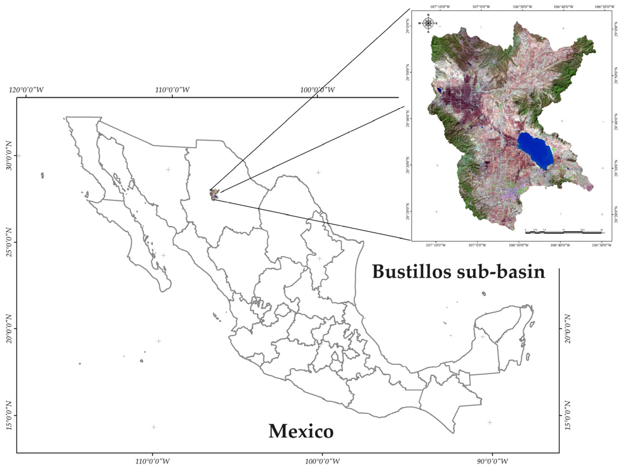
2.1. Study Area

The study area, denominated “Bustillos sub-basin”, is located in the municipality of Cuauhtémoc, Chihuahua, Mexico. Figure 1 shows a composite image of the Bustillos sub-basin from Landsat 8 and its geographic location within Mexico. Its geographical limits are between the coordinates 28°13′ and 28°59′ north latitude and 106°34′ and 107°10′ west longitude. The basin covers an area of 3264 km2 and ranges in altitude from 1960 to 2800 m. According to CONAGUA [38], the climate is semiarid, temperate, and with a mean annual precipitation of 407.15 mm, while the temperatures range between 14.6 °C and 38 °C. The Bustillos sub-basin is part of the physiographic province of the Sierra Madre Occidental, characterized by volcanic rocks from the Tertiary period. On a smaller scale, the sub-basin is located in the Sierras and Llanuras Tarahumaras sub-province (covering 80% of the area) and the Gran Meseta and Cañones Chihuahuenses [39]. The natural recharge of the sub-basin’s aquifer comes from rainfall (horizontal underground flow to the aquifer) and infiltration induced by irrigation return flows [39]. The predominant vegetation types are grasslands and agricultural lands with crops such as maize, beans, and oats. Nevertheless, at higher altitudes, natural and induced grasslands, desert scrub, pine–oak, oak–pine, and oak forests predominate [40].
From 1970 to 2020 the population in Cuauhtemoc grew by 170.18%. The largest increases were recorded from 1980 to 1990 and from 2000 to 2010. Meanwhile, the registered change of croplands grew by 140% in the same period. The most impressive growth in the region was recorded in the irrigated agricultural area, which grew from 1737.6 hectares in 1970 to 49,789.30 ha in 2020 [18,19,20,21]. This represents an increment of 2765.40% for the last 50 years (Table 1).

2.2. Data Sources

For the analysis of the land use changes in the study area, satellite images from the Landsat platform were downloaded from the department portal of the United States Geological Survey (USGS) (https://glovis.usgs.gov, accessed on 1 February 2022). The changes were evaluated for two time periods: November 1974 and October 2016. Due to the time frame of 43 years, information from sensors Landsat MSS and Landsat OLI Collection 2, Level 1 (C2L1) had to be obtained. The spatial resolution of both images was 30 m. After downloading, geographic and radiometric correction [32,41] was performed using QGIS 3.v 3.26 program. Table 2 summarizes the information of the images used.

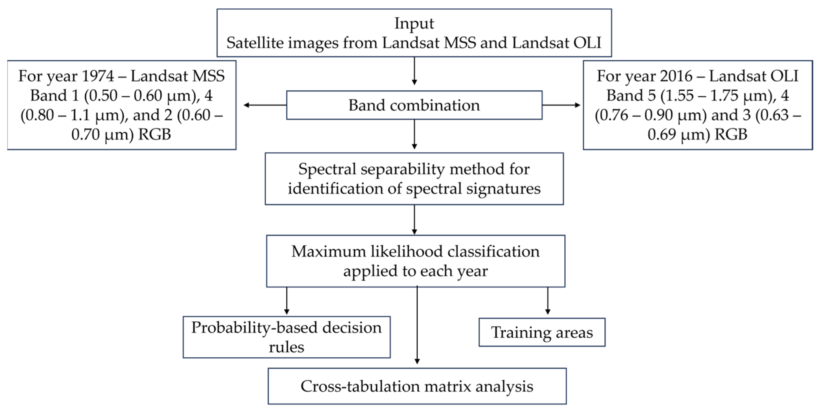
2.3. Image Processing

After the preprocessing of the satellite images, the preparation for the land use change analysis continued (Figure 2). Initially, it is necessary to combine the bands [42] to obtain a false-color image. Hence, for each year, i.e., 1974 and 2016, a pertinent selection and combination of bands allowed for highlighting important terrain attributes. This facilitated the analysis and visual delimitation of land covers on the ground. The next step was to identify the spectral signatures in the satellite images [32] to cluster them in categories associated with the different terrain components [31]. The spectral separability method [43] was used for this purpose. This process minimizes the standard deviation of readings from each band to avoid confusion in category identification. After this, the maximum likelihood classification method was applied, for which training areas categorized by an expert were used. The supervised classification consists of assigning a value to each pixel in the image according to the land use identified by an expert [44]. The use of classification machine learning models in studies of LULC has significantly increased [30,32,45,46].
This technique is considered efficient since it assumes that the data follow a normal distribution when assigning a probability to each pixel belonging to a class [47,48,49]. The identification of training areas was defined using the data obtained from the field vegetation characterization, databases from INEGI [39] (Series V), and expert interpretation of satellite images. For each year, the supervised classification method was applied using training areas and probability-based decision rules. This method calculates the probability of each pixel belonging to a category based on its spectral signature (Equation (1)).
g i x = I n   p   m i 1 2   I n   | i | 1 2 x m i T     i 1 ( x m i )
where gi = class, x = number of bands, p (mi) = probability that class mi appears in the image and is assumed by all classes, |∑i| = determinant of the covariance matrix, ∑ i1 = inverse matrix, and m = vector.

2.4. Classification Accuracy

The Kappa coefficient was used to validate the classifications (Equation (2)) by employing 360 control points for each year taken from the false-color composites. The Kappa coefficient and the error matrix are considered common techniques in measuring the accuracy of thematic maps generated by the classification process [50]. Measurements of particular categories of classification can be verified with field data or reference data [51].
K h a t = N X i i X i + X + i   N 2 X i + X + i    
where KAPPA = Kappa index; k = number of matrix files; Xii = observation number on row i and column i (along the diagonal); Xi+ and X + i = total marginal for row i and column i, respectively; and N = total number of observations.

2.5. Change Analysis

After the supervised classification of each image (1974 and 2016), a cross-tabulation matrix analysis was performed, and the method developed by Pontius et al. [52] was applied to estimate the rate of change of each category. This method allows for analyzing the area that covers each category presented by year and identifying the most relevant surface transitions. In the matrix design [53], the rows represent the surface area in year 1 (1974), while the columns refer to the surface area of the categories in year 2, i.e., 2016 (Table 3). Finally, the last column represents the proportion of the landscape that experienced losses in category i between time 1 and time 2. Similarly, the last row provides information on the proportion of category j that experienced gains between time 1 and time 2. To identify the surface area that changes from one category to another, showing persistence on the diagonal of the matrix, the observed values matrix is compared with the expected values matrix generated randomly using the chi-square equation.
X 2 = i = 1 j j = 1 j { N × [ P i j ( P i + × P + j ) ] 2 ( P i + × P + j ) }  
where Pij represents the proportion of a land use transitioning from category i to category j, with J being the number of categories, Pij on the diagonal denotes the proportion of land use that shows persistence in category j, and the rest of the cells indicate transition from category i to a different category j. Pi + represents the proportion of land use in category i at time 1, which is the sum over all j of Pij. P + j, where the proportion of land use in category j at time 2, which is the sum over i of Pij. N is the number of cells in the grid map.
For a more detailed analysis regarding losses and gains, Pontius et al. [52] suggest generating a second table. This table represents the net and total change, as well as exchanges, gains, and losses between categories (Table 4).
Gain (Gj) is the difference between the total area of category j at time 2 (L + j) and the persistence expressed on the diagonal of the matrix (Pjj).
G   j = L + j   L i j
Loss (L) is the difference between the total area of category i at time 1 (Li) and the persistence (Lij).
L = L i + L i j
The net change (NC) is defined as the absolute value of the difference between losses and gains in each category.
  N C = |   L G |
The total change at the category level (TC) is obtained by adding the net change (NC) and the exchange (Exc), or alternatively, by summing up gains (Gj) and losses (L).
T C = N C + E x c
The exchange (Exc) represents the loss of a specific category in one location accompanied by its simultaneous gain in another location; it is twice the minimum value of gains or losses.
2 * M I N ( L , G J )

3. Results

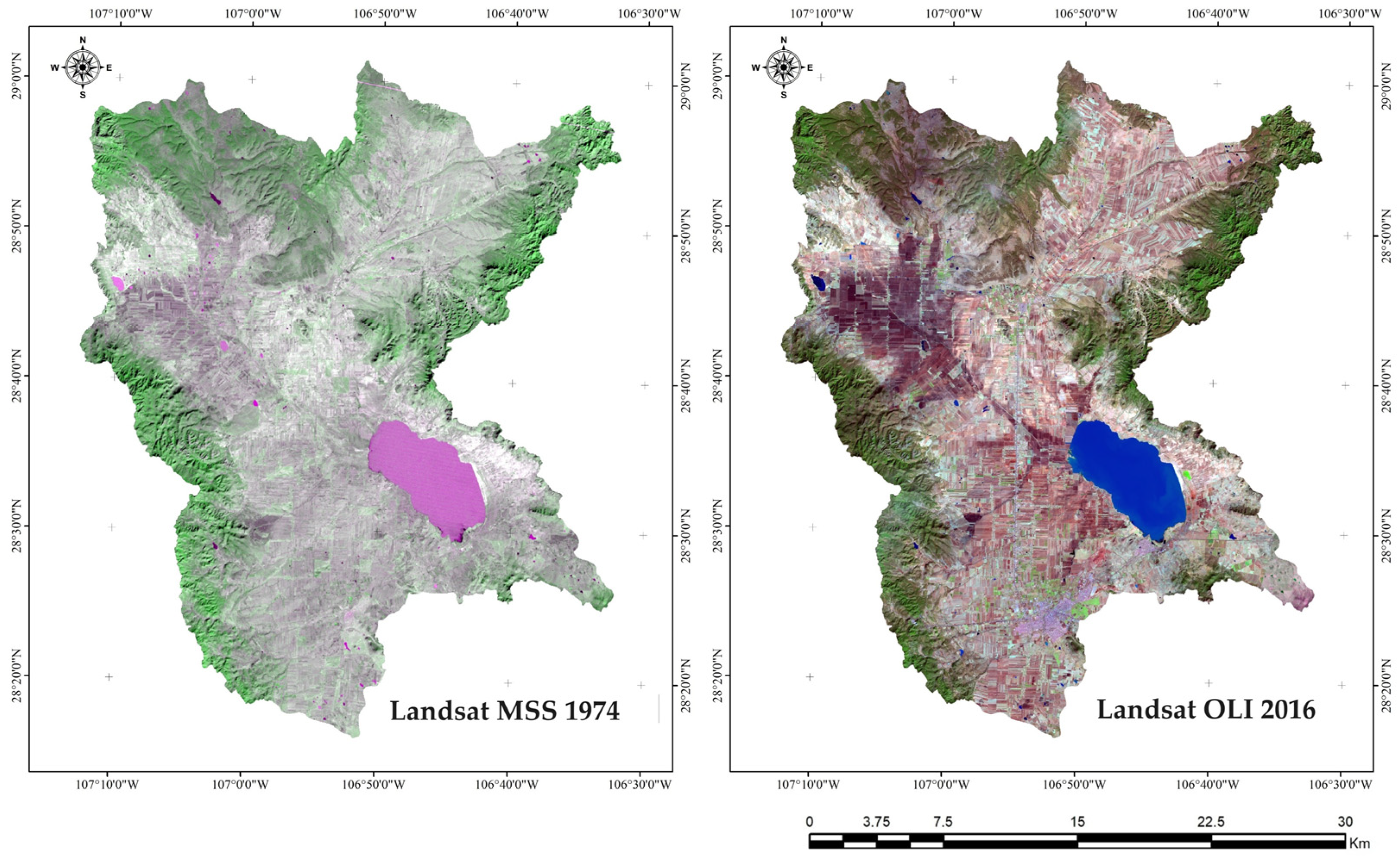
3.1. False-Color Images

When analyzing land use, an important process is the generation of false-color composites from satellite images. Figure 3 shows the false-color composite image of 1974, which was generated by combining bands 1 (0.50–0.60 µm), 4 (0.80–1.1 µm), and 2 (0.60–0.70 µm) in the visible spectrum range RGB (Red, Green, and Blue) from the Landsat MSS sensor. Additionally, Figure 3 presents the result of band composition for the year 2016 where bands 5 (1.55–1.75 µm), 4 (0.76–0.90 µm), and 3 (0.63–0.69 µm) were used in the RGB order for Landsat OLI satellite.

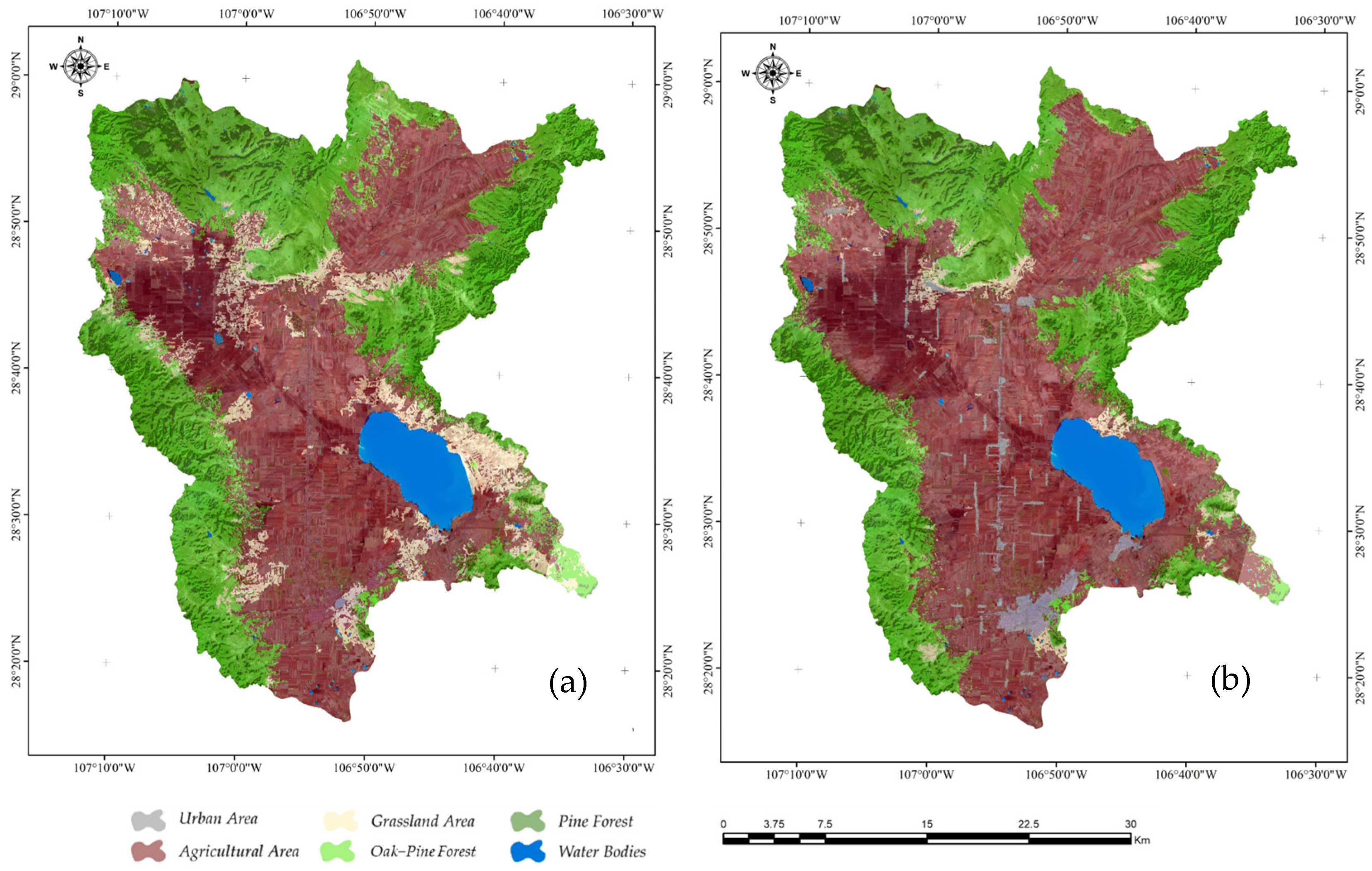
3.2. Land Use Classification

Two types of land use were determined for the study area, as they were the most representative of the region. The land use of agricultural areas presented the least spatial distribution in the study area. The land use classification of 1974 presented the largest errors. The estimated global precision, based on the error matrix, was 94% with a kappa index of 0.92. In this year, the lowest precision was presented by the class of oak–pine forest; the producer precision was 90%, and the user precision was 89%. For the year 1974, the global precision was 92%, with a kappa index of 0.90 (see Table 5).

3.3. Land Use Changes

In both years, the resulting land uses were urban areas, agricultural areas, grasslands, oak–pine forests, pine forests, and water bodies (Figure 4). For the year 1974, the most abundant land uses (Table 6) were agricultural lands covering 153,575 ha, followed by oak–pine forests with 112,216 hectares. In contrast, the class with the smallest area was urban areas, with 142 hectares. In the year 2016, the land use classes were distributed as follows: agriculture had 176,162.82 ha, forest communities covered 123,509.23 ha, human settlements occupied 7993.34 ha, and grasslands had 6893.24 hectares. Additionally, Table 6 shows the differences in land use areas between the classifications of 1974 and 2016. Grassland areas had the most significant change, decreasing by 20,990.62 hectares, followed by oak–pine forests, which lost 8608.56 hectares, and pine forests with a reduction of 586.7 hectares. Additionally, water bodies decreased by 228.02 hectares. Urban areas had an increase of 7851.78 hectares, while agricultural areas expanded by 22,577.71 hectares. Figure 5 presents the percentage distribution of land use in the Bustillos sub-basin for the years 1974 and 2016. A clear urbanization process over a period of 43 years can be observed, which represented a total of 98% by 2016. The distribution in agricultural areas was 47% in 1974, and by 2016 it was 53%. On the other hand, grasslands changed from 80% to 20%.
Table 7 shows the results of the transition processes from the cross-tabulation matrix [53]. The classes that remained unchanged are on the diagonal of the matrix, while the values outside the diagonal represent the changes. Table 8 and Figure 6 represent the land use change processes in the Bustillos sub-basin from 1974 to 2016. Over 43 years, there was an anthropic permanence of 141.86 hectares. Agricultural areas transitioned to urban areas for 5756.41 ha, while 1938.55 ha of grasslands became urban zones. Additionally, 156.52 ha of oak–pine forest were transformed into human settlements. These changes signify a notable increase in this category. The conversion of land for crops is another important factor in land use changes [11,16]. In this case, a considerable area (19,446.73 ha) of grasslands was converted to agricultural land. Similarly, 8598.85 ha of oak–pine forest were deforested and converted to agricultural land, as well as 60.64 ha of pine forest. Special attention is given to the increment in agricultural lands over water bodies, driven by the rising water demand due to the expansion of agriculture and urban zones. In the Bustillos sub-basin, 228.02 ha of water bodies were converted to agricultural lands. Some changes are due to ecological succession, as is the case of the oak–pine forest converting to grasslands (394.67 ha). The pine forest was also degraded, as 526.05 ha transitioned to oak–pine forest.

3.4. Gains, Losses, and Exchanges of the Categories

To analyze the spatial dynamics, it is necessary to calculate gains, losses, and exchanges. Table 9 estimates a total change of 74,212.85 hectares. The urban areas presented gains of 7851.48 ha, and there was no urban exchange with other categories; thus, the total and net changes were equal. Agricultural areas gained 28,334.23 ha, grasslands 394.67 ha, and oak–pine forest 526.05 ha of surface change. In these classes, the total change is greater than the net change. This is because the total change is the sum of gains and losses. On the other hand, net change cannot identify spatial transitions, as it derives from the difference in the surface between 1974 and 2016. In the mentioned categories, despite the surface remaining almost equal on both dates, the surface exchange among classes resulting from gains and losses determined their spatial variation, making these categories the ones with the most significant changes in the territory. Finally, pine forests (586.69 ha) and water bodies (228.02 ha) only had losses. The category with the most relevant change was agricultural lands, indicating that the change from this class to urban areas is permanent. It is important to analyze the total changes for each class, as this allows for calculating the systematic changes in the territory and not just absolute change values. This results in a better perception of reality [54]. Ultimately, it is relevant to mention that the most affected classes are due to urban growth and agricultural land expansion.

4. Discussion

4.1. False-Color Composites and Classes Delimitation

This present study confirms the usefulness of false-color composites. Additionally, it was able to accurately delineate urban areas in a semiarid, temperate climate. This is significant because some features in semiarid zones share similar spectral signatures, making the delineation process more complex [55]. In this case, the precise identification of categories can also be attributed to the urban area being surrounded by agricultural lands with no fallow, as urban zones can be confounded with fallow cropland [56]. Therefore, studies in similar climatic zones should consider the effect of this factor when choosing the images to analyze. This also highlights the importance of natural and human drivers such as the seasonality of vegetation and cultivation cycles in the process of delineation [56,57]. Here, the satellite images analyzed were from November 1974 to October 2016, corresponding to the season with high net primary productivity (NPP). This clearly distinguishes the agricultural lands from urban zones. However, the accuracy has to be improved. Briceño [58], in a study conducted in the Sierra Tarahumara using Landsat images for land use classification, highlighted the importance of false-color composition for discriminating land uses such as agricultural lands, grasslands communities, pine forests, and human settlements, among others. Additionally, composite images can identify areas where vegetation cover has been lost in forest and agricultural areas [59]. Therefore, the implementation of composite images for land use evaluation [60,61] provides results that establish this technique as reliable in detecting vegetation cover.
Our selected method, maximum likelihood, proved to be efficient in distinguishing the different classes even though it has been reported to show a limitation in features with similar spectra [45]. Antillon-Veleta et al. [62] applied this classification method in the same study area. They distinguished four categories, i.e., water bodies, agriculture, bare soil, and forests, reporting a great spectral variability in the category of bare soil. In our case, we were able to delimitate urban areas. This can be attributed, as discussed above, to the lack of fallow croplands, which may facilitate the distinction of spectra between urban areas and surrounding land uses. Our methodology can serve as a base for future studies aiming at urban planning that considers the natural vocation of the territory. In this manner, sustainable urbanization, as proposed in the SDG 11, can be achieved. Importantly, this urban planning can promote resilient communities in the face of climate change, especially when droughts are becoming more recurrent in the Bustillos basin. In another study, Manjarrez et al. [63], using spectral data from the Landsat TM 5 in the Chihuahuan Desert, were able to demonstrate the sensor’s capacity to identify eight land use and vegetation classes in three land use and vegetation maps for the State of Chihuahua for the years 1990, 2000, and 2012.

4.2. Land Use Changes and Implications

García et al. [64] quantified the dynamic changes in the south–central region of Mexico over a period of 27 years. Unlike the Bustillos sub-basin, where there was an increase of 22,577.71 ha in agricultural lands, their monitoring showed a decrease in this type of land use. The changes were reported due to the abandonment of these areas, the incorporation of livestock, and urban growth. In our study region, the inefficiency of furrow irrigation has been reported as one of the reasons for the expansion of agricultural fields [65]. On the other hand, Prieto et al. [66], analyzed the land use change dynamics between 1989 and 2014 in a micro-basin in Chihuahua city. Their results revealed a gradual increase in urban areas of up to 38%. In the Bustillos sub-basin, in 43 years, there was an increment of 7851.48 hectares. This can be partially attributed to the closeness to the locality of Anahuac, part of Cuauhtemoc municipality, which has had an important population growth [18,19,20,21], and to the presence and expansion of industries. Specifically, the agroindustry sector is an important economic activity in the area. However, this has resulted in an increment of coliform bacteria in water bodies originating from sewage [67]. The expansion of urban areas is not exclusive to Mexico. Rawat and Kumar [68] evaluated land use changes in Almora, India, using remote sensing and GIS-based techniques and found that over the last two decades, urbanized areas increased by 3.55% (9.48 km2). Their results also revealed a decrease of 1.52% (4.06 km2) in agricultural lands. The rapid rates of urbanization can increase the land surface temperature (LST), leading to the formation of an urban heat island [69].
Locally, land use change studies show reductions in natural areas, which could have implications for ecosystem services. For instance, Pool et al. [4] observed a 6.04% increase in croplands over five years in the Valles Centrales, resulting in the destruction of 69,240 hectares of grasslands. Likewise, the Conchos River basin has been impacted by agriculture at the expense of forests and grasslands [70]. Furthermore, our results show several deforestation processes, such as the conversion of grasslands, pine, and oak–pine forests to agricultural areas. This can have implications in the Bustillos Lagoon, an important wetland in the Bustillos sub-basin fed by streams from the high areas of the basin [22]. Our study demonstrates that over a period of 43 years, some of these areas have been converted to croplands, potentially decreasing aquifer recharge. Other causes of the degradation of this and other water bodies of the area are poor agricultural practices as reported by A la Torre et al. [65], such as overgrazing, garbage from households, and pollution [71]. Additionally, in the face of a more intense hydrological cycle and intense rainfall events due to climate change [5], soil water erosion can increment and add more sediment load to the lagoon. Previously, a reduction of 40 cm in the depth of the lagoon due to sedimentation was reported [71]. Erosion is an alarming form of land degradation previously reported in Chihuahua [4,70,72]. Hence, prevention measures should be taken at these high areas of the Bustillos sub-basin. Lastly, land use changes in arid and semiarid zones can risk water security [73].
Our results and methodology based on remote sensing techniques can support the creation of a land use plan that considers the distribution of land uses according to the topography of the sub-basin. This will prevent, for instance, erosion from higher areas restricting the sedimentation of water bodies. Another implication of this strategy could be the reduction of agrochemical pollution coming from the industries. Likewise, this study can be useful for restoration plans by considering the locations of grasslands, oak–pine forests, and pine forests, as of the year 1974. Future research on the area could focus on the formation of urban heat islands and the implementation of complex models such as S.W.A.T. This can support further mitigation and restoration programs in the Bustillos sub-basin. Additionally, land use change studies at interval levels are encouraged, as shorter periods of time could allow for a better understanding of how socio–economic factors shape land-use changes.

5. Conclusions

This study focused on analyzing the dynamics of LULC over a period of 43 years in the Bustillos basin using remote sensing and the method of maximum likelihood. The results demonstrate an expansion of agricultural lands and a significant urban growth. These land uses gained a total of 28,334.23 and 7851.48 ha, respectively. This highlights a lack of land planning that does not consider the conservation of natural ecosystems. For instance, 8598.85 hectares of oak–pine forest were lost to agriculture and 156.52 ha due to urban expansion. Additionally, the pine forests lost a total of 586.69 hectares. Grasslands were also affected, losing 21,385.28 ha, and from which, 19,446.73 hectares were converted to agriculture and 1938.55 to urban zones. The loss of 228.02 hectares of water bodies is relevant due to the semiarid conditions of the area. This is related to agricultural activities, agricultural intensification, and growth of human settlements, which were later affected by water shortages due to the recurrent droughts. The degradation and deforestation of natural environments in the Bustillos basin is alarming. The consequences are already documented (e.g., high erosion rates, sedimentation of water bodies, and chemical pollution), and these are likely to continue if the dynamics shown in this work, i.e., agricultural expansion and urban growth, remain. Hence, our study serves as a basis to develop responsible proposals that both respect the natural vocation of the territory and ensure the livelihood of the communities. Furthermore, we promote the use of geospatial tools and techniques to promote alternatives and strategies. This approach will strengthen the agri-food sector, mitigate climate change, and facilitate adaptation efforts.

Author Contributions

Conceptualization, G.V.-Q. and S.V.-G.; methodology, G.V.-Q. and M.M.-S.; software, N.S.H.-Q.; writing original draft preparation, M.C.N.-R. and M.C.V.-A.; supervision, G.V.-Q.; writing review and editing, F.M.-L. and P.M.L.-S. All authors have read and agreed to the published version of the manuscript.

Funding

This research received no external funding.

Data Availability Statement

The original contributions presented in the study are included in the article, further inquiries can be directed to the corresponding author.

Acknowledgments

We sincerely thank the National Council for Science and Technology of Mexico (CONAHCYT) for the scholarship provided to the first author of this manuscript to pursue his PhD program.

Conflicts of Interest

The authors declare no conflicts of interest.

References

  1. Perring, M.P.; De Frenne, P.; Baeten, L.; Maes, S.L.; Depauw, L.; Blondeel, H.; Carón, M.M.; Verheyen, K. Global environmental change effects on ecosystems: The importance of land-use legacies. Glob. Change. Biol. 2016, 22, 1361–1371. [Google Scholar] [CrossRef]
  2. Fifth National Climate Assessment, Changes in Climate and Land Use Affect Land-System Resilience. Available online: https://nca2023.globalchange.gov/chapter/6/ (accessed on 17 June 2024).
  3. Borrelli, P.; Robinson, D.A.; Panagos, P.; Lugato, E.; Yang, J.E.; Alewell, C.; Wuepper, D.; Montanarella, L.; Ballabio, C. Land use and climate change impacts on global soil erosion by water (2015–2070). Proc. Natl. Acad. Sci. USA 2020, 117, 21994–22001. [Google Scholar] [CrossRef]
  4. Pool, D.B.; Panjabi, A.O.; Macias-Duarte, A.; Solhjem, D.M. Rapid expansion of croplands in Chihuahua, Mexico threatens declining North American grassland bird species. Biol. Conserv. 2014, 170, 274–281. [Google Scholar] [CrossRef]
  5. Schiavina, M.; Melchiorri, M.; Corbane, C.; Florczyk, A.J.; Freire, S.; Pesaresi, M.; Kemper, T. Multi-scale estimation of land use efficiency (SDG 11.3. 1) across 25 years using global open and free data. Sustainability 2019, 11, 5674. [Google Scholar] [CrossRef]
  6. Díaz Caravantes, R.; Bravo Peña, L.C.; Alatorre Cejudo, L.C.; Sánchez Flores, E. Geospatial Analysis of the Interaction between Land and Water Use in the Peri-Urban Area of Cuauhtémoc, Chihuahua: A Socio-Environmental Study in Northern Mexico. Investig. Geogr. Boletín 2014, 83, 117–131. [Google Scholar] [CrossRef]
  7. Hasan, S.S.; Zhen, L.; Miah, M.G.; Ahamed, T.; Samie, A. Impact of land use change on ecosystem services: A review. Environ. Dev. 2020, 34, 100527. [Google Scholar] [CrossRef]
  8. United Nations. Transforming Our World: The 2030 Agenda for Sustainable Development; The Strategic Plan 2020–2023; United Nations, Department of Economic and Social Affairs Habitat, U.N.: New York, NY, USA, 2019. [Google Scholar]
  9. United Nations (UN)-Hábitat. La Dimensión Urbana de los Objetivos de Desarrollo Sostenible. Available online: https://onuhabitat.org.mx/ (accessed on 15 October 2023).
  10. Maja, M.M.; Ayano, S.F. The impact of population growth on natural resources and farmers’ capacity to adapt to climate change in low-income countries. Earth Syst. Environ. 2021, 5, 271–283. [Google Scholar] [CrossRef]
  11. Foley, J.A.; Defries, R.; Asner, G.P. Global Consequences of Land Use. Science 2005, 309, 570–574. [Google Scholar] [CrossRef]
  12. Clarity and Leadership for Environmental Awareness and Research (CLEAR Center). Cattle and Land Use: The Differences between Arable Land and Marginal Land and How Cattle Use Each. Available online: https://clear.ucdavis.edu/explainers/cattle-and-land-use-differences-between-arable-land-and-marginal-land-and-how-cattle-use (accessed on 18 February 2024).
  13. Viana, C.M.; Freire, D.; Abrantes, P.; Rocha, J.; Pereira, P. Agricultural land systems importance for supporting food security and sustainable development goals: A systematic review. Sci. Total Environ. 2022, 806, 150718. [Google Scholar] [CrossRef]
  14. Foley, J.; Ramankutty, N.; Brauman, K.; Cassidy, E.S.; Gerber, J.S.; Johnston, M.; Mueller, N.D.; O’Connell, C.; Ray, D.K.; West, P.C.; et al. Solutions for a Cultivated Planet. Nature 2011, 478, 337–342. [Google Scholar] [CrossRef]
  15. McGarigal, K.; Tagil, S.; Cushman, S.A. Surface metrics: An alternative to patch metrics for the quantification of landscape structure. Landsc. Ecol. 2009, 24, 433–450. [Google Scholar]
  16. Secretaría de Medio Ambiente y Recursos Naturales (SEMARNAT). Información Adicional al Trámite SEMARNAT-02-001 Solicitud de Autorización de Cambio de Uso de Suelo en Terrenos Forestales. Gobierno de México. Available online: https://www.gob.mx/semarnat/documentos/tramite-semarnat-02-001 (accessed on 15 February 2021).
  17. López-Vazquez, V.H.; Balderas, P.M.; Chávez, M.C.; Perez, J.J.; Gutiérrez, C.G. Cambio de uso de suelo e implicaciones socioeconómicas en un área mazahua del altiplano mexicano. CIENCIA Ergo-Sum 2015, 22, 136–144. [Google Scholar]
  18. INEGI (Instituto Nacional de Estadística Geografía e Informática). Subsistema de Información Demográfica y Social. Censos y Conteos de Población y Vivienda. 2024. Available online: https://www.inegi.org.mx/programas/ccpv/1970/#publicaciones (accessed on 20 July 2024).
  19. SADER (Secretaría de Agricultura y Desarrollo Rural). Servicio de Información Agroalimentaria y Pesquera (SIAP), Datos Abiertos. Chihuahua, México. 2024. Available online: http://infosiap.siap.gob.mx/gobmx/datosAbiertos.php (accessed on 20 July 2024).
  20. INEGI (Instituto Nacional de Estadística Geografía e Informática). V Censo Agrícola Ganadero y Ejidal 1970. Dirección General de Estadística. México. 1975. Available online: https://www.inegi.org.mx/contenidos/productos/prod_serv/contenidos/espanol/bvinegi/productos/historicos/1329/702825111144/702825111144_1.pdf (accessed on 19 July 2024).
  21. INEGI (Instituto Nacional de Estadística Geografía e Informática). Dirección General de Difusión. In Cuaderno Estadístico Municipal Cuauhtémoc Chihuahua 2001; INEGI (Instituto Nacional de Estadística Geografía e Informática): Chihuahua, Mexico, 2002; 174p. [Google Scholar]
  22. Conociendo la Laguna de Bustillos. Available online: https://storymaps.arcgis.com/stories/45b00034bc9942bcbe5e9ee6c4bd6b3d (accessed on 17 June 2024).
  23. Comisión Nacional Para el Conocimiento y Uso de la Biodiversidad (CONABIO). 37 Lago Bustillos. Available online: http://www.conabio.gob.mx/conocimiento/regionalizacion/doctos/rhp_037.html (accessed on 18 July 2024).
  24. A la Torre, L.C.; García, A.K.; Rodríguez, A.J.; Erives, V.; González, E. Estimación de la erosión potencial de la cuenca laguna de Bustillos, Chihuahua, Mexico. Dialnet 2014, 249–258. [Google Scholar]
  25. Zhu, L.; Suomalainen, J.; Liu, J.; Hyyppä, J.; Kaartinen, H.; Haggren, H. A review: Remote sensing sensors. Multi-Purp. Appl. Geospat. Data 2018, 19. [Google Scholar] [CrossRef]
  26. Vázquez-Quintero, G.; Solís-Moreno, R.; Pompa-García, M.; Villarreal-Guerrero, F.; Pinedo-Alvarez, C.; Pinedo-Alvarez, A. Detection and projection of forest changes by using the Markov Chain Model and Cellular Automata. Sustainability 2016, 8, 236. [Google Scholar] [CrossRef]
  27. Flores, S.E.; Yool, S.R. Sensitivity of change vector analysis to land cover change in an arid ecosystem. Int. J. Remote Sens. 2007, 28, 1069–1088. [Google Scholar] [CrossRef]
  28. Verburg, P.H.; Crossman, N.; Ellis, E.C. Land system science and sustainable development of the earth system: A global land project perspective. Anthropocene 2015, 3, 29–41. [Google Scholar] [CrossRef]
  29. Al-sharif, A.A.; Pradhan, B. Monitoring and Predicting Land Use Change in Tripoli Metropolitan City Using an Integrated Markov Chain and Cellular Automata Models in GIS. Arab. J. Geosci. 2014, 7, 4291–4301. [Google Scholar] [CrossRef]
  30. Talukdar, S.; Singha, P.; Mahato, S.; Pal, S.; Liou, Y.A.; Rahman, A. Land-use land-cover classification by machine learning classifiers for satellite observations—A review. Remote Sens. 2020, 12, 1135. [Google Scholar] [CrossRef]
  31. Phan, T.N.; Kuch, V.; Lehnert, L.W. Land cover classification using Google Earth Engine and random forest classifier—The role of image composition. Remote Sens. 2020, 12, 2411. [Google Scholar] [CrossRef]
  32. MohanRajan, S.N.; Loganathan, A.; Manoharan, P. Survey on Land Use/Land Cover (LU/LC) change analysis in remote sensing and GIS environment: Techniques and Challenges. Environ. Sci. Pollut. R. 2020, 27, 29900–29926. [Google Scholar] [CrossRef]
  33. Nasa Earth Observatory. Available online: https://earthobservatory.nasa.gov/features/FalseColor (accessed on 16 June 2024).
  34. Pinedo, A.C.; Pinedo, A.A.; Martinez, Q.R.M. Análisis de áreas deforestadas en la región centro-norte de la Sierra Madre Occidental, Chihuahua, México. Tecnociencia Chihuah. 2007, 1, 36–43. [Google Scholar] [CrossRef]
  35. Segura, F.; Tricando, M.M. Evolución del paisaje y estado de conservación de la reserva forestal de Valdivia. Land 2003, 19, 197–209. [Google Scholar]
  36. Rimal, B.; Zhang, L.; Keshtkar, H.; Haack, B.; Rijal, S.; Zhang, P. Land use/land cover dynamics and modeling of urban land expansion by the integration of cellular automata and markov chain. ISPRS Int. J. Geo-Inf. 2018, 7, 154. [Google Scholar] [CrossRef]
  37. Food and Agriculture Organization of the United Nations (FAO). Base Referencial Mundial del Recurso Suelo. In Informes Sobre Recursos Mundiales del Suelo; FAO: Rome, Italy, 2015; Volume 106. [Google Scholar]
  38. Comisión Nacional del Agua (CONAGUA). Registro Público de Derechos de Agua. Available online: https://www.gob.mx/conagua (accessed on 15 October 2023).
  39. Instituto Nacional de Estadística y Geografía (INEGI). Censo General de Población y Vivienda, Instituto Nacional de Estadística, Geografía e Informática, México. Available online: https://www.inegi.org.mx (accessed on 15 October 2023).
  40. Comisión Nacional para el Conocimiento y Uso de la Biodiversidad (CONABIO). La Biodiversidad en Chihuahua: Estudio de Estado. 2014. Available online: https://www.biodiversidad.gob.mx/region/EEB/estudios/ee_chihuahua (accessed on 15 October 2023).
  41. Markham, B.L.; Arvidson, T.; Barsi, J.A.; Choate, M.; Kaita, E.; Levy, R.; Lubke, M.; Masek, J.G. Comprehensive Remote Sensing; Elsevier: Amsterdam, The Netherlands, 2018; pp. 27–90. [Google Scholar] [CrossRef]
  42. Gonzalez, L.; Yamamoto, H. The wall: The Earth in true natural color from real-time geostationary satellite imagery. Remote Sens. 2020, 12, 2375. [Google Scholar] [CrossRef]
  43. Jiang, H.; Eastman, J.R. Application of Fuzzy Measures in Multi-Criteria Evaluation in GIS. Int. J. Geogr. Inf. Sci. 2000, 14, 173–184. [Google Scholar] [CrossRef]
  44. Awotwi, A.; Anornu, G.K.; Quaye-Ballard, J.A.; Annor, T. Monitoring Land Use and Land Cover Changes Due to Extensive Gold Mining, Urban Expansion, and Agriculture in the Pra River Basin of Ghana, 1986–2025. Land Degrad. Dev. 2018, 29, 3331–3343. [Google Scholar] [CrossRef]
  45. Yang, C.; Wu, G.; Ding, K.; Shi, T.; Li, Q.; Wang, J. Improving land use/land cover classification by integrating pixel unmixing and decision tree methods. Remote Sens. 2017, 9, 1222. [Google Scholar] [CrossRef]
  46. Kafy, A.A.; Shuvo, R.M.; Naim, M.N.H.; Sikdar, M.S.; Chowdhury, R.R.; Islam, M.A.; Sarker, H.S.; Khan, H.H.; Kona, M.A. Remote sensing approach to simulate the land use/land cover and seasonal land surface temperature change using machine learning algorithms in a fastest-growing megacity of Bangladesh. Remote Sens. Appl. Soc. Environ. 2021, 21, 100463. [Google Scholar] [CrossRef]
  47. Valero Medina, J.A.; Alzate Atehortúa, B.E. Comparison of maximum likelihood, support vector machines, and random forest techniques in satellite images classification. Rev. Tecnura 2019, 23, 13–26. [Google Scholar] [CrossRef]
  48. Pineda-López, R.; Febvre, N.; Martínez, M. Importancia de proteger pequeñas áreas periurbanas por su riqueza avifaunística: El caso de Mompaní, Querétaro, México. Huitzil, Revista Mex. Ornitol. 2010, 11, 69–80. [Google Scholar]
  49. How Maximum Likelihood Classification Works. Esri. Available online: https://desktop.arcgis.com/en/arcmap/latest/tools/spatial-analyst-toolbox/how-maximum-likelihood-classification-works.htm (accessed on 26 May 2024).
  50. Smits, P.C.; Dellepiane, S.G.; Schowengerdt, R.A. Quality assessment of image classification algorithms for land-cover mapping: A review and a proposal for a cost-based approach. Int. J. Remote Sens. 1999, 20, 1461–1486. [Google Scholar]
  51. Congalton, R.G.; Oderwald, R.G.; Mead, R.A. Assessing Landsat classification accuracy using discrete multivariate analysis statistical techniques. Photogramm. Eng. Remote Sens. 1983, 49, 1671–1678. [Google Scholar]
  52. Pontius, R.G., Jr.; Shusas, E.; McEachern, M. Detecting important categorical land changes while accounting for persistence. Agric. Ecosyst. Environ. 2004, 101, 251–268. [Google Scholar] [CrossRef]
  53. Pontius, R.G., Jr.; Cheuk, M.L. A generalized cross-tabulation matrix to compare soft-classified maps at multiple resolutions. Int. J. Geogr. Inf. Sci. 2006, 20, 1–30. [Google Scholar] [CrossRef]
  54. Ibarra-Bonilla, J.S.; Villarreal-Guerrero, F.; Prieto-Amparán, J.A.; Santellano-Estrada, E.; Pinedo-Alvarez, A. Characterizing the impact of Land-Use/Land-Cover changes on a Temperate Forest using the Markov model. Egypt. J. Remote Sens. Space Sci. 2021, 24, 1013–1022. [Google Scholar] [CrossRef]
  55. Ali, K.; Johnson, B.A. Land-use and land-cover classification in semi-arid areas from medium-resolution remote-sensing imagery: A deep learning approach. Sensors 2022, 22, 8750. [Google Scholar] [CrossRef]
  56. Lasanta, T.; Vicente-Serrano, S.M. Complex land cover change processes in semiarid Mediterranean regions: An approach using Landsat images in northeast Spain. Remote Sens. Environ. 2012, 124, 1–14. [Google Scholar] [CrossRef]
  57. Wang, J.; Bretz, M.; Dewan, M.A.A.; Delavar, M.A. Machine learning in modelling land-use and land cover-change (LULCC): Current status, challenges and prospects. Sci. Total Environ. 2022, 822, 153559. [Google Scholar] [CrossRef]
  58. Briceño-Hidalgo, Y.I. Análisis Espacio Temporal del Cambio de Uso de Suelo en Bosques Templados de la Sierra Tarahumara, Chihuahua. Bachelor’s Thesis, Autonomous University of Chihuahua (UACh), Chihuahua, Mexico, 2020. [Google Scholar]
  59. Hilker, T.M.; Wulder, N.; Coops, J.; Linke, G.; McDermid, J.; Masek, F.; Gaoy, J.C. A new data fusion model for high spatial- and temporal-resolution mapping of forest disturbance based on Landsat and MODIS. Remote Sens. Env. 2009, 113, 1613–1627. [Google Scholar] [CrossRef]
  60. Healey, S.P.; Cohen, W.B.; Zhiqiang, Y.; Krankina, O.N. Comparison of Tasseled Cap-based Landsat data structures for use in forest disturbance detection. Remote Sens. Env. 2005, 101, 301–310. [Google Scholar] [CrossRef]
  61. Lemenkova, P. Robust vegetation detection using RGB colour composites and isoclust classification of the Landsat TM image. Geomat. Landmanag. Land. 2021, 147–167. [Google Scholar]
  62. Antillon, M.Y.; Corral, G.M.; A la Torre, L.C. Análisis de los Cambios de Cobertura y Uso de Suelo en los Márgenes de la Laguna de Bustillos Chihuahua: Efectos de la Expansión Agrícola. Available online: https://www.uacj.mx/CGTI/CDTE/JPM/Documents/SELPER/assets/m005.pdf (accessed on 7 July 2024).
  63. Manjarrez-Domínguez, C.; Pinedo-Alvarez, A.; Pinedo-Alvarez, C.; Villarreal-Guerrero, F.; Cortes-Palacios, L. Cortes-Palacios, L. Vegetation Landscape Analysis due to Land Use Changes on Arid Lands. Pol. J. Ecol. 2015, 63, 272–279. [Google Scholar] [CrossRef]
  64. García Nieto, H.; García Daguer, R.R.; Moreno Sánchez, R.; González Ramos, A. Using Remote Sensors and GIS to Delimit Changes in Agricultural Land Use from 1970 to 1997 in the State of Guanajuato. Invest. Geog 2002, 47, 92–112. [Google Scholar]
  65. A la Torre, L.C.; Granados, A.; Bravo, L.C.; Torres, M.E.; Wiebe, L.C.; Uc, M.I.; González, M.O.; Sánchez, E.; Rojas, H.L.; Salas, V. Ineficiencia de riego rodado agrícola en la cuenca de la laguna de Bustillos, Chihuahua, México: Características geométricas de las parcelas agrícolas y abatimiento del acuífero. Tecnol. Cienc. Agua 2019, 10, 241–281. [Google Scholar] [CrossRef]
  66. Prieto-Amparán, J.A.; Pinedo-Alvarez, A.; Villarreal-Guerrero, F.; Pinedo-Alvarez, C.; Morales-Nieto, C.; Manjarrez-Domínguez, C. Past and future spatial growth dynamics of Chihuahua city, Mexico: Pressures for land use. ISPRS Int. J. Geo-Inf. 2016, 5, 235. [Google Scholar] [CrossRef]
  67. Amado-Álvarez, J.P.; Pérez-Cutillas, P.; Ramirez-Valle, O.; Alarcón-Cabañero, J.J. Análisis de la calidad del agua en las lagunas de Bustillos y de los mexicanos (Chihuahua, México). Papeles De Geogr. 2016, 62, 107–118. [Google Scholar] [CrossRef]
  68. Rawat, J.S.; Kumar, M. Monitoring Land Use/Cover Change Using Remote Sensing and GIS Techniques: A Case Study of Hawalbagh Block, District Almora, Uttarakhand, India. Egypt. J. Remote Sens. Space Sci. 2015, 18, 77–84. [Google Scholar] [CrossRef]
  69. Sadiq Khan, M.; Ullah, S.; Sun, T.; Rehman, A.U.; Chen, L. Land-use/land-cover changes and its contribution to urban heat Island: A case study of Islamabad, Pakistan. Sustainability 2020, 12, 3861. [Google Scholar] [CrossRef]
  70. Martínez-Sifuentes, A.R.; Villanueva-Díaz, J.; Estrada-Ávalos, J.; Vázquez-Vázquez, C.; Orona-Castillo, I. Soil loss and runoff modification caused by land use change in the Conchos River basin, Chihuahua. Nova Sci. 2020, 12. [Google Scholar] [CrossRef]
  71. Ducks Unlimited of Mexico (DUMAC). The Current State of the Bustillos Lagoon behind the Ecological Disaster. Available online: https://dumac.org/2024/07/25/la-laguna-de-bustillos-detras-del-desastre-ecologico/ (accessed on 30 July 2024).
  72. De la Maza-Benignos, M.; Banda-Villanueva, I.; Mendoza-González, G.; Leal-Nares, O.A.; Rendón-Herrera, G. Reporte del estado de los pastizales del Desierto Chihuahuense. Pronatura Noreste-Am. Bird Conserv. 2019. [Google Scholar]
  73. Rafiei-Sardooi, E.; Azareh, A.; Shooshtari, S.J.; Parteli, E.J. Long-term assessment of land-use and climate change on water scarcity in an arid basin in Iran. Ecol. Model. 2022, 467, 109934. [Google Scholar] [CrossRef]
Figure 1. Location of the study area. Bustillos sub-basin located in Chihuahua state in northern Mexico.
Land 13 01320 g001
Figure 2. Flowchart of image processing.
Land 13 01320 g002
Figure 3. False-color composition of Landsat MSS image and Landsat OLI 8 image.
Land 13 01320 g003
Figure 4. Land use in the years (a) 1974 and (b) 2016.
Land 13 01320 g004
Figure 5. Distribution of land use as a percentage for the years 1974 and 2016 in the Bustillos sub-basin. AA, agricultural areas; GA, grassland areas; OPF, oak–pine forest; PF, pine forest; UA, urban areas; WB, water bodies; A2016 area year 2016; A1974, area year 1974.
Land 13 01320 g005
Figure 6. Analysis of land use and vegetation changes by category from 1974 to 2016 in the Bustillos sub-basin.
Land 13 01320 g006
Table 1. Changes in population and agricultural land in the Bustillos basin.
Variable1970198019902000200320102020
Population66,856.0085,589.00112,589.00124,378.00NA154,639.00180,638.00
P.G.R. (%)NA28.0231.5510.47NA24.3316.81
Total Land Crop113,366.00NA113,400.00267,800.00NA272,390.00NA
Rainfed Agr.111,395.00NA77,432.0067,767.0067,005.0064,156.7773,517.00
Irrigation Agr.1737.60NA33,186.0040,192.0045,879.4546,393.9149,789.30
Planted area113,132.60NA110,618.00107,959.00112,844.45110,550.00123,306.30
This information corresponds to the municipality of Cuauhtemoc, Chihuahua. P.G.R. (Population Growth Rate), Agr. (Agriculture), NA (Not Available). Data from INEGI and SADER.
Table 2. Data sources.
DataDate% CloudData SourceSpatial Resolution
Landsat MSSNovember 19740Global Visualization Viewer (GloVis) from the USGS.
https://glovis.usgs.gov
30 m × 30 m
Landsat OLIOctober 20160GloVis from the USGS.
https://glovis.usgs.gov
30 m × 30 m
Table 3. Cross tabulation matrix.
Time 2Total Year 1Loss
Category 1Category 2Category 3Category 4
Time 1
Category 1P11P12P13P14P1+P1 ± P11
Category 2P21P22P23P24P2+P2 ± P22
Category 3P31P32P33P34P3+P3 ± P33
Category 4P41P42P43P44P4+P4 ± P44
Total year 2P + 1P + 2P + 3P + 41
GainP + 1 − P11P + 2 − P22P + 3 − P33 P + 4 − P44
Table 4. Transition matrix of estimated values between categories.
Loss
(L)
Gain
(Gj)
Exchange
(Exc)
Net Change
(NC)
Total Change
(TC)
L1 ± L11L + 1−L112 × MIN (L,Gj)TC − ExcL + Gj or
L2 ± L22L + 2−L22 Exc + NC
Table 5. Accuracy assessment of the classified land use maps.
Year/Land UseClassification Accuracy
Producer’s Accuracy (%)User’s Accuracy (%)Overall Accuracy (%)Cohen’s Kappa
1974 920.90
Urban Area8988
Agricultura Areas9392
Grassland9291
Oak–Pine Forest9191
Pine Forest9291
Water Body9594
2016 940.92
Urban Area9090
Agricultura Areas9493
Grassland9393
Oak–Pine Forest9089
Pine Forest9190
Water Body9696
Table 6. Surface area (Ha) and changes of land use and vegetation types for 1974 and 2016.
Land Use19742016Difference 2016–1974
Urban Area141.867993.347851.48
Agricultura Areas153,585.11176,162.8222,577.71
Grassland 27,883.866893.24−20,990.62
Oak–Pine Forest112,216.05103,607.49−8608.56
Pine Forest20,488.4419,901.74−586.7
Water Body12,851.9112,623.89−228.02
Total327,167.23327,182.52
Table 7. Cross-tabulation matrix to compare land use changes between the years 1974 and 2016.
UAAAGAOPFPFWBTOTALLOSS
UA141.8600000141.860.00
AA5756.41147,827.340000153,583.755756.41
GA1938.55194,46.736498.4200027,883.7021,385.28
OPF156.528598.85394.67103,063.3400112,213.379150.03
PF060.640526.0519,900.47020,487.1624586.69
WB0228.0200012,623.8512,851.87228.02
TOTAL7993.34176,161.56916893.08752103,589.38619,900.473212,623.853
GAIN7851.4828,334.23394.67526.050.000.00
UA = Urban areas; AA = Agricultural areas; GA = Grassland areas; OPF = Oak–pine Forest; PF = Pine Forest; WB = Water bodies.
Table 8. Land use change processes from 1974 to 2016 in the Bustillos sub-basin.
Dynamics of ChangesType of Change Area
Persistence of urban areas Anthropic persistence141.86
Agricultural land to urban areas Urbanization 5756.41
Grasslands to urban areas Urbanization 1938.55
Oak–pine Forest to urban areas Urbanization 156.52
Persistence of agricultural areas Permanence 147,827.34
Grasslands to agricultural landsDeforestation19,446.73
Oak–pine Forest to agricultural landsDeforestation8598.85
Pine forest to agricultural landsDeforestation60.64
Water bodies to agricultural landsOthers228.02
Grasslands persistenceNatural persistence6498.42
Oak–pine Forest to grasslandsDegradation394.67
Oak–pine Forest persistenceNatural persistence103,063.34
Pine forest to oak–pine forestDegradation526.05
Pine forest persistence Natural persistence19,900.47
Water bodies Natural persistence12,623.85
Table 9. Matrix of estimated exchange, total change, net change, gain, and loss between categories from 1974 to 2016.
GainsLossesExchangesNet ChangeTotal Change
Urban Areas7851.480.000.007851.487851.48
Agricultural Areas28,334.235756.4111,512.8222,577.8234,090.64
Grasslands394.6721,385.28789.3320,990.6121,779.94
Oak–pine Forest526.059150.031052.108623.989676.08
Pine forest0.00586.690.00586.69586.69
Water bodies0.00228.020.00228.02228.02
Total37,106.4237,106.4213,354.2460,858.6074,212.85
Disclaimer/Publisher’s Note: The statements, opinions and data contained in all publications are solely those of the individual author(s) and contributor(s) and not of MDPI and/or the editor(s). MDPI and/or the editor(s) disclaim responsibility for any injury to people or property resulting from any ideas, methods, instructions or products referred to in the content.

