Abstract
Soil erosion and hydrogeological risk are critical phenomena gaining increased recognition within the scientific community. Although these occurrences are naturally occurring, human activities can exacerbate their impacts. For example, deforestation consistently amplifies soil erosion. This study examines two distinct forest management strategies aimed at addressing soil erosion: the Banded Standards Method (BSM) and the Scattered Standards Method (SSM). We conducted a field experiment in two test areas located in central Italy, with one area employing the BSM and the other implementing the SSM. Two soil erosion plots were established, representing prototypes of a novel erosion monitoring apparatus called the Natural Erosion Trap (NET), or Diabrosimeter, specifically designed for forest environments. At regular intervals, particularly after significant storm events, sediment and leaf litter accumulated within the erosion plots were collected, dried, and weighed to quantify erosion rates and assess the efficacy of the silvicultural methods under investigation. The results revealed a 30.72% reduction in the eroded material with BSM compared to SSM, underscoring BSM’s ability to mitigate potential hazards and preserve environmental integrity.
1. Introduction
Soil erosion and hydrogeological risk represent critical phenomena garnering increasing attention from the scientific community [1,2,3] as well as international and national regulatory bodies [4,5,6], owing to their profound ramifications on human livelihoods, infrastructure integrity, and ecological balance [5,7,8,9]. While both phenomena are inherently natural, anthropogenic activities often exacerbate their severity [10,11,12,13,14,15]. For instance, deforestation invariably triggers soil erosion and, contingent upon the geomorphological characteristics of the affected area, may precipitate hydrogeological instability [16,17,18]. Over time, numerous empirical investigations have been undertaken to understand soil erosion dynamics [19]. Pioneering work in this domain was conducted by Wischmeier and Smith [20,21], who, following years of experimental research, formulated the Universal Soil Erosion Equation (USLE).
This equation remains the cornerstone in soil erosion modelling, notably in its revised iteration, the Revised Universal Soil Loss Equation (RUSLE) [22,23]. Indeed, the genesis of this formula stemmed from extensive experimental endeavours predominantly within agricultural contexts [24]. The widespread adoption of the USLE (or RUSLE) framework for regional applications underscores its enduring utility [25].
To determine the equation, the researchers devised experimental plots with cemented sides terminating in water and sediment collectors, representing a widely employed setup in experimental fields. A comprehensive review revealed that the majority of such experiments have been conducted within agricultural contexts [26,27]. However, investigations into soil erosion estimation within forested areas utilizing experimental plots remain relatively scarce, with only a limited number of studies examining the effects of logging on soil dynamics [17,28,29]. In recent years, the predominant approach in natural environment research pertaining to soil erosion has shifted towards modelling within a Geographic Information System (GIS) framework, leveraging the Revised Universal Soil Loss Equation (RUSLE) [30,31,32,33,34,35].
Nevertheless, a significant challenge in such a modelling approach lies in the scarcity of detailed input data. Notably, commonly utilized digital elevation models, typically with a resolution of 30 m, lack representation of soil microtopography, potentially leading to oversimplified terrain characterization and erroneous erosion estimations. Consequently, the paucity of experimental studies on forest soil erosion primarily stems from the logistical challenges associated with constructing experimental plots. Notably, conventional plot construction techniques [20,21,36] are associated with notable environmental impacts, including substantial soil disturbance, introduction of artificial elements incongruent with natural settings, and significant financial outlay.
Italy stands out as one of Europe’s most hydrologically vulnerable nations, with 94% of its administrative regions grappling with various forms of hydrological instability according to the ISPRA Report on hydrogeological instability [37]. This predicament is poised to exacerbate in the coming years, particularly under the spectre of climate change, which forecasts a marked reduction in average rainfall alongside an uptick in extreme weather events, potentially escalating the frequency and severity of hydrological disturbances such as floods [6,38].
Italy’s geographical landscape is characterized by 41.6% hilly terrain, 35.2% mountainous regions, and a mere 23.2% flat land, predominantly occupied by urban settlements. Natural ecosystems, including forests, are predominantly situated in hilly and mountainous terrains. Consequently, owing to the Mediterranean precipitation patterns prevalent in the country, Italy witnesses a notably higher average annual soil erosion rate within forested areas compared with other European regions, as elucidated by Borrelli et al. [17]. Specifically, Italian forest ecosystems exhibit an average annual soil erosion rate of 0.33 t/ha/yr, surpassing the rates observed in Mediterranean forests (0.18 t/ha/yr) and other European counterparts (0.003 t·ha−1·yr−1).
Given the substantial proportion (42.3%) of Italian forest cover comprising coppice forests, which inherently engender greater soil erosion compared with high stand forests, it becomes imperative to devise silvicultural strategies aimed at mitigating post-harvest soil erosion and subsequent hydrological instability. In pursuit of this objective, we investigate the efficacy of the Banded Standards Method (BSM), a silvicultural coppice method hypothesized by Del Favero [39] and conceptually scrutinized by our research team [40].
The primary distinction between the two coppice forest management techniques lies in the arrangement of the trees that remain in the forest after logging, known as standards. In the Scattered Standards Method (SSM), these standards are dispersed throughout the logged area. This method ensures that the trees are evenly spread, providing a more uniform structure to the forest after logging operations. In contrast, the BSM arranges the standards in a band or stripe that runs parallel to the contour lines of the terrain. This technique creates a more organized and systematic layout, concentrating the remaining trees in specific areas and following the land’s natural topography.
The BSM can make forest management practices, such as replanting and maintenance, more efficient because of the organized layout of the standards. By following the contour lines, this method can also help in reducing soil erosion and managing water flow more effectively, as the trees act as barriers to slow down runoff. This approach can be particularly advantageous in areas prone to erosion or with uneven terrain. Because of the band of standards that act as an ecological corridor, this method can also bring a reduction in the loss of animal and plant biodiversity and can ensure the conservation of gene flows. Those stripes can act also as wind barriers, so they can reduce the wind effect followed by the logging, and finally, they hide the view of the bare areas better, simulating a seamless covering of the slopes with a real improvement at the landscape level.
To evaluate the viability of the BSM, we conducted a field experiment wherein two test areas were established as follows: one employing the conventional SSM, typical in Italian coppice forest management, and the other implementing the BSM.
The experiment was carried out within a mixed coppice forest situated in Maiella National Park. After logging activities, two soil erosion plots were installed, each covering one of the logged areas. These soil erosion plots represent prototypes of a novel erosion monitoring apparatus termed the Natural Erosion Trap (NET) or Diabrosimeter, specifically designed for forest environments. At regular intervals, and particularly following significant storm events, sediment and leaf litter accumulated within the erosion plots were collected, dried, and weighed to quantify erosion rates and assess the efficacy of the silvicultural methods under investigation.
2. Materials and Methods
2.1. Study Area
The study area (Figure 1) is situated within the “Gole di Popoli” in the Municipality of Popoli, in the Abruzzo Region (central Italy). The site is part of Maiella National Park and of the State Natural Reserve “Mt. Rotondo” (42°11′20.78″ N; 13°50′57.24″ E). The altitudinal range of the area spans from 308 m to 332 m above sea level, characterized by an average slope of 48.5%, moderate ruggedness, and a predominant northeast-facing aspect. Geophysical data obtained from Geoportale Abruzzo [41] indicate that the study area exhibits typical physiographic features and lithological composition consistent with sloping terrain containing valleys and calcareous substrates. Specifically, the area is typified by Middle–Late Jurassic limestones and calcarenites, with radiolarian and filaments-like remains [42].
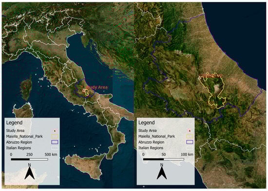
Figure 1.
The figure shows the location of the study area. On the left is its location on a national scale, while its location on a regional scale is on the right. The Abruzzo Region is highlighted in blue, the contour of Maiella National Park is highlighted in yellow, and the study area is highlighted in red. The image on the right is a satellite orthophoto of the region.
Regarding climatic aspects, the area can be classified in the temperate macroclimate, temperate oceanic sub-Mediterranean bioclimate with upper subhumid ombrotype, and upper mesotemperate thermotype [43]. According to the Köppen–Geiger climate classification, the study area has a temperate climate with hot summers and no dry seasons (symbol Cfa) [44]. The average annual rainfall is 719.6 mm, with an average of 86 rainy days in a year [45]. The maximum collected rainfalls are 36.4 mm (1 h) and 177.4 mm (24 h). The rainiest seasons are spring (April) and autumn (October, November, and December).
The minimum rainfall is in July (25.8 mm). The average daily temperature is 13.5 °C, with average maximum temperatures exceeding 30.0 °C in the summer months (absolute maximum 45.0 °C) and average minimum temperatures ranging between 0.1 °C and 0.8 °C during the coldest months (absolute minimum −17.0 °C). All climatic data refer to the thermopluviometric station of Popoli (UTM WGS84: 32T 899738.33E, 4678532.80N) for the period 1951–2000 [45] (Figure 2).
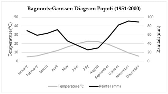
Figure 2.
Bagnouls–Gaussen diagram of the study area during the period 1951–2000.
According to the phytosociological classification, the study area is covered by a mixed deciduous broadleaf forest dominated by Quercus pubescens Willd. belonging to the plant association Roso sempervirentis–Quercetum virgilianae with elements of Mediterranean sclerophyllous vegetation (Quercus ilex L., Viburnum tinus L., Ruscus aculeatus L., Smilax aspera L., etc.) of the class Quercetea ilicis [46,47].
2.2. Silvicultural Treatment
The forest underwent coppicing using the “coppice with standards” method. In one plot, standards were released onto the ground utilizing the SSM, the most prevalent technique in coppicing. Conversely, the other plot employed the BSM as proposed by Schirone et al. [40]. This method involves releasing standards in stripes perpendicular to the steepest slope direction, thereby altering conventional coppicing geometry. It was specifically designed to manage steep coppice forests and mitigate soil erosion following logging activities.
A field campaign was conducted in the logged area to assess the main characteristics of vegetation within the two plots. Data on the number of plants categorized into standards and stumps, the number of shoots, and their respective diameters (DBH) were collected (Table 1). The mean height of the trees, determined through direct measurement of selected logged trees, was recorded at 14 m (Table 1). Plot 1 (P1) corresponds to the area where the SSM was implemented, while Plot 2 (P2) represents the BSM plot. The average diameter of Plot P1 was 7.76 cm, the one in Plot P2 was 8.58 cm, and their mean was 8.17 cm. The diameter was calculated at breast height (1.30 m) for each standard and shoot with a diameter superior to 3 cm. All the standards, stumps, and shoots were counted. By summing the number of the standards with the number of the shoots, we obtained the total number of stems present in the two plots. Finally, the results were compared in hectares and then summed. Plot P1 resulted to have 88 standards (1760/ha) and 65 shoots (1300/ha) for a total of 153 stems (3060/ha). Plot P2 resulted to have 79 standards (1580/ha) and 69 shoots (1380/ha) for a total of 148 stems (2960/ha). The sum of the two plots was 167 standards (1670/ha), 134 shoots (1340/ha), and. in total, 301 stems (3010/ha).

Table 1.
Summary of the principal characteristics of the 2 plots and in total. The first two lines show the average diameter (DBH) and height of the standing trees, and the other lines represent data on the number of plants, in their categories. The results were reported for both, as they were counted and compared to hectares. Finally, the basal area and the volume of the trees inside the plots are provided.
The coppice cutting of the two plots was carried out between the end of September and the end of October 2022, by releasing 140 standards per hectare. Given that each plot was 500 square meters, 7 trees (standards) were left in each plot (see Figure 3).
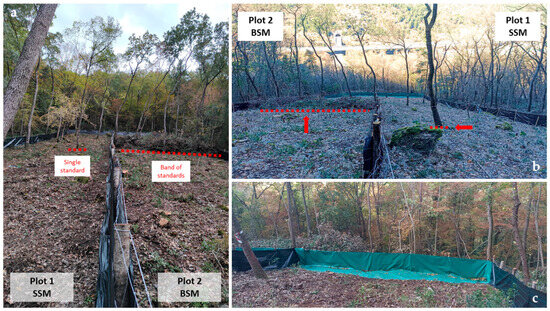
Figure 3.
Views of silvicultural treatments applied in the study area: (a) the bottom shows Plot P1 on the left, which employs the Scattered Standards Method (SSM), while Plot P2 on the right uses the Banded Standards Method (BSM); (b) the top shows plot P2 (BSM) on the left and plot P1 (SSM) on the right. In plot P1, the typical standards disposition is visible, while in P2, the band of standards and the bundles of twigs are positioned on their bases; and (c) a detailed view from above of the PVC collector installed at the bottom of the cut area. In red, a detail of the comparison sections between the two methods.
In the first plot (SSM), the standards were dispersed throughout the study area, ensuring the representation of each species within the plot. The species, diameter (DBH), and height of these standards are detailed in Table 2. In the second plot (BSM), the standards were strategically positioned to form a single stripe (band) in the middle of the area, running parallel to the shorter side and approximately 25 m from both the base and the top of the plot. The two plots were modelled in three dimensions using the LiDAR module of an iPhone 14 pro combined with the PolyCam app [48], and the resulting models are included in the Supplementary Materials (Figures S1 and S2). Species differentiation was not considered; instead, standards were selected solely for inclusion in the designated band of standards (refer to Table 2). For this reason, in Plot P2, only two species remained (Quercus pubescens Wild. and Fraxinus ornus L.), while in Plot P1, four species remained (Quercus pubescens Wild., Quercus ilex L., Ostrya carpinifolia Scop., and Acer monspessulanum L.) (Table 2). Brushwood resulting from limbing activities was piled on the upper side of the standards band to further mitigate water runoff and act as a barrier against rocks of varying sizes, reducing the risk of hazards to humans.
Table 2.
This table summarizes the main characteristics of the standards left after logging. Species, diameter (DBH), and height are noted. In particular, the standards inside Plot P1 (SSM) are shown on the left and those in Plot P2 are shown on the right (BSM).
2.3. Hydrological and Geological Data
Recognizing that soil erosion within a specific area is influenced significantly by both the rainfall regime and soil properties [21], we conducted thorough analyses on these factors. For the rainfall regime assessment, we utilized data obtained from a rain gauge station of the Abruzzo Hydrological Centre (Centro Funzionale e Ufficio Idrologia, Idrografico, Mareografico–Agenzia di Protezione Civile della Regione Abruzzo) situated near the study area.
Our examination focused on the daily rainfall and temperature readings recorded at the station, spanning from November 2022 to December 2023. Furthermore, we employed the 2023 dataset to construct a 2023 Bagnouls–Gaussen diagram (Figure 2), enabling us to grasp the climatic variances between 2023 and the data averages spanning 1951 to 2000 [45].
In terms of soil analysis, a comprehensive field campaign was undertaken, during which we collected four soil samples from each plot. With the utmost care, the initial 20 cm were extracted by samplings at a distance of 12.5 m in a 30 × 30 cm plot. These samples were subsequently subjected to analysis to determine key soil parameters, including texture, Total Organic Carbon (TOC), and Soil Organic Matter (SOM). The findings of these soil analyses are presented in Table 3.
Table 3.
Summary of the soil analysis. The results are shown in percentage (%). The samples were taken every 10/15 m, from the bottom to the top of the plots, in the central parts.
2.4. Experimental Plot
Following the logging activities, we introduced a novel erosion control mechanism known as the Natural Erosion Trap (NET) or Diabrosimeter. This choice stemmed from the necessity for a larger plot compared with traditional Wischmeier soil erosion plots, measuring 22.13 m in length and 1.83 m in width [49]. The forested study area demanded a larger footprint than agricultural settings because of the general high biodiversity and the presence of trees and their expansive canopies, which significantly influence erosion dynamics. Thus, there was a clear need for a solution that could be easily installed and removed, had minimal environmental impact, could adapt to various terrains including protected areas, and effectively mitigate risks associated with falling rocks within the study site.
The NET prototype was meticulously engineered to intercept water runoff, sediment, rocks, and organic debris. Its adaptable design facilitates deployment across diverse environmental conditions, accommodating variable slopes, and allowing customization in terms of shape and size to meet specific research objectives (see Figure 4).
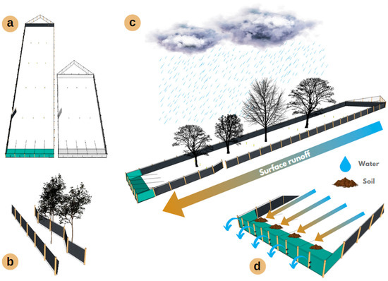
Figure 4.
Features and operation of the NET erosion plot prototype: (a) plot length can be modulated; (b) plot perimeter can be easily adjusted to suit different environmental conditions; (c) the system operates by channelling surface runoff towards the base of the plot following rainfall events; (d) the collector receives water and eroded soil, with the soil settling while the water flows through nozzles.
The initial prototype we constructed features a rectangular configuration, with its shorter sides aligned parallel to contour lines and the longer sides perpendicular to these lines. Divided into two primary sections, the first serves as a protective barrier, effectively isolating the plot from its surroundings, while the second functions as the primary collection unit.
The protective barrier comprises a sturdy metallic mesh to shield the plot from external rockfall and other debris, complemented by a mulching film that serves to prevent the ingress of water and sediment. This fencing component spans three sides of the plot, encompassing the top and longer edges.
Meanwhile, the collector section incorporates a reinforcing net structure along with a heavy-duty 900 g/m2 waterproof PVC tarpaulin, acting as the sediment collection apparatus. Both sections are affixed to wooden poles positioned along the perimeter at regular intervals, approximately two meters apart.
For installation, the fencing component is vertically embedded into the soil, while the collector’s net is similarly inserted vertically. The PVC tarpaulin is partially secured horizontally to the soil, with its upper section buried about 10 cm deep, and the remainder fixed in conjunction with the net.
Additionally, the vertical section of the collector can accommodate nozzles, facilitating either water runoff collection or functioning as a relief valve (refer to Figure 5).
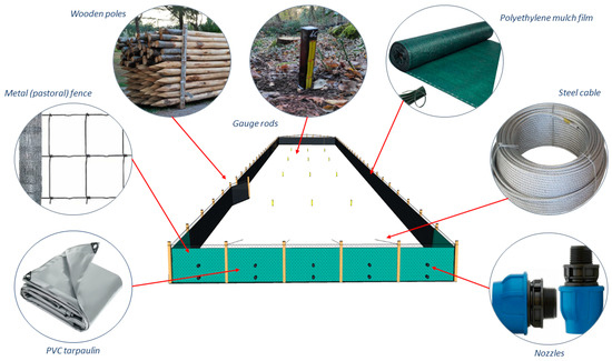
Figure 5.
Overview of the erosion plot prototype’s elements.
The vertical section of the collector effectively intercepts water and assorted sediments, while the horizontal component facilitates the flow of water and sediment toward the vertical portion. The robust fencing and the substantial PVC tarpaulin ensure that even sizable rock fragments are impeded, safeguarding the system from damage. Various methods exist for sediment retrieval, contingent upon forest type and topography. Options include employing nozzles connected to tubing and tanks for sediment and water collection, or, alternatively, blocking the nozzles and utilizing a pump to extract water and sediment into tanks. In the absence of water, sediment can be directly retrieved from the collector. Additionally, depending on research objectives, pegs can be installed using the soil erosion peg method depicted in Figure 5 [50,51,52,53].
2.5. Collection and Analysis Methodologies
The research team manually conducted the removal of sediments and leaves accumulated by the two NETs over the period from November 2022 to December 2023. This task typically involved two operators. The first operator accessed the site via a side entrance positioned in the middle of the left long side of the plot, cautiously minimizing ground disturbance while navigating along the perimeter to reach the collector. Meanwhile, the second operator remained outside the plot.
The picking process unfolded systematically, progressing from left to right in a prescribed sequence. Initially, surface materials, predominantly dead leaves, were gathered and placed into numbered bags. Next, residual water accumulated within the collector was suctioned out using a pump and stored in numbered tanks. Subsequently, sediment accumulated at the bottom of the collector was retrieved and stored in numbered containers. This sequence was repeated for the adjacent experimental plot, adhering to the same operational protocol.
Once the sediment, residual water, and leaves were removed from the plots, they were transported to the laboratory for further analysis. Initial processing involved cleaning the leaves to eliminate any adhering sediment, also to prevent potential fermentation within the bags. This cleaning procedure entailed soaking the leaves in water, followed by thorough cleaning, drying, and subsequent weighing after each collection.
Regarding sediment analysis, samples collected directly from the plots were naturally dried or oven-dried as appropriate. Sediment suspended in water tanks underwent a decanting process to separate the solid components, after which it was dried and combined with other sediment samples. Subsequent differentiation classified sediment into gravel (particles with a diameter greater than 2 mm) and fine sediment (particles with a diameter less than 2 mm, including sand, loam, and clay), achieved through the use of pedological sieves. The weights of the two sediment types were recorded and summed for each plot.
3. Results and Discussion
The two NETs plots commenced operations effectively from 4 November 2022, continuing until 14 December 2023, spanning approximately 13 months. To ensure a meaningful comparison between the two plots and to accurately convert the erosion results into square meters and hectares, we initially determined their respective areas and slopes. Plot P1 (SSM) exhibited a mean slope of 47.1% and covered an area of 373 m2, while Plot P2 (BSM) featured a mean slope of 49.03% and occupied an area of 435 m2. The combined average slope for both plots was calculated at 48.17%. As for leaf collection, we conducted multiple weightings throughout the year, whereas sediment weight measurements were undertaken only three times during the entire year.
Leaf Collection
After the initial leaf collection, a notable disparity became evident between the two plots. Plot P1, managed using the SSM, amassed a greater quantity of leaves compared with Plot P2, where the BSM was applied. Plot P1 accumulated a total leaf weight of 6.4 kg, whereas Plot P2 amassed 3.8 kg.
These findings, however, did not factor into the variation in slope between the two plots. To address this, we adjusted the results proportionally, considering the slope. Consequently, the weighted leaf mass of Plot P1 experienced a slight increase, rising from 6.4 kg to 6.6 kg, while Plot P2 saw a decrease, dropping from 3.8 kg to 3.7 kg. Subsequently, we divided the adjusted sum by the respective plot areas, revealing soil loss rates of 0.018 kg/m2 for Plot P1 (SSM) and 0.008 kg/m2 for Plot P2 (BSM). Notably, the BSM exhibited a 55.5% reduction in leaf loss compared to the SSM (Table 4).
Table 4.
Weighing results of the leaf collection. The first column shows the total rainfall that led to leaf loss. The second and third columns show the results for Plot P1 and Plot P2, respectively. Each weight is associated with the date of collection.
After the first process of weighing, we investigated the rainfall that generated the leaf loss. Thanks to the data provided by the rain gauge of the Abruzzo Hydrological Centre (Centro Funzionale e Ufficio Idrologia, Idrografico, Mareografico–Agenzia di Protezione Civile della Regione Abruzzo), we could correlate the leaf loss inside the two plots with the rainfall that generated that loss. As evident, there exists a substantial correlation among rainfall, seasonal variations, and leaf loss. Particularly, during November and December, an important leaf loss is observed, closely associated with both rainfall and the seasonal shedding typical of broadleaf forests. Despite potentially lower rainfall levels during this period compared with others, the majority of leaf shedding occurs, as exemplified by the January collection, which yielded more leaves than that of 16 February. This trend persists throughout the year, with consistent leaf loss occurring even during periods of relatively lower total rainfall. Consequently, there is a continual loss of organic matter throughout the year, emphasizing the ongoing impact of leaf shedding on forest ecosystems (Table 5 and Figure 6).
Table 5.
Sediment weight from Plot P1 (SSM) and Plot P2 (BSM).
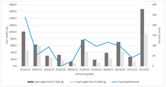
Figure 6.
Relationship between rainfall and leaf loss, and the difference in leaf loss between the two plots. Plot P1 is represented by the dark grey column, while Plot P2 is represented by the light grey column.
Table 5 and Figure 6 clearly show that Plot P2 experienced a decrease in the loss of leaves, suggesting that this plot has a blocking effect on leaves, so it could reduce the organic matter loss.
Regarding the sediment collected by the two erosion plots, we faced limitations in conducting the same procedure as that used for the leaves. We could only conduct three weightings throughout the year, allowing us to establish correlations with rainfall and seasonal variations. Recognizing the significance of differentiating sediment types—rock fragments, which, depending on their size, can pose risks to human health, and fine sediment, which affects only soil fertility—we initially categorized the collected sediment into gravel (with a diameter larger than 2 mm) and fine sediment (including sand, loam, and clay).
The results of this differentiation revealed that in Plot P1 (SSM), we collected 4508.1 g of gravel and 3698.4 g of fine sediment, while in Plot P2 (BSM), we collected 3486.2 g of gravel and 5039 g of fine sediment. Similar to the leaves, we adjusted the collected sediment weights based on slope and area to obtain values in kg/ha.
For Plot P1 (SSM), erosion rates were calculated at 123.5 kg/ha for gravel and 101.3 kg/ha for fine sediment, totalling 224.8 kg/ha. In Plot P2 (BSM), the erosion rates were 78.8 kg/ha for gravel and 113.9 kg/ha for fine sediment, with a total erosion of 192.6 kg/ha. Notably, the BSM exhibited lower erosion rates overall, with a 19% decrease in total soil erosion. While gravel erosion consistently favoured Plot P1, fine sediment erosion initially favoured Plot P2, though this trend equalized over the year.
The final weighing showed a decrease in fine sediment erosion in Plot P2, attributed to its enhanced anti-erosive capacity one year post-logging, suggesting better forest recovery and subsequent erosion mitigation. The results show promising differences. For a better comprehension of the results, Table 5 shows the Plot P1 and Plot P2 results.
Apart from mitigating leaf and soil losses, the BSM demonstrated effectiveness in averting large rock displacement. While Plot P1 experienced no obstructions from rocks, Plot P2 intercepted numerous rocks successfully.
By integrating standards with bundled twigs, the method effectively prevented the movement of six rocks, collectively weighing 90.35 kg. Notably, these blocked rocks encompassed varying weights, including heavy ones, underscoring the method’s pivotal role in ensuring human safety.
The results underscore the method’s ability to address broader concerns beyond soil erosion. By obstructing rocks, the BSM mitigates potential hazards and preserves environmental integrity, demonstrating its versatility across diverse terrains. Its successful application in Plot P2 highlights its adaptability to challenging conditions, validating its efficacy in sustainable land management.
Continued research and implementation of the BSM offer promise in mitigating soil erosion and enhancing environmental resilience. Integrating findings from this study into land management practices can inform the development of more robust erosion control strategies, ensuring the long-term health and sustainability of ecosystems globally.
The ability of the BSM to effectively block rocks complements its other benefits, making it a comprehensive solution for mitigating various forms of land degradation and promoting ecosystem health.
After converting all measurements to tons per hectare (t/ha), we conducted a comprehensive analysis of sediment accumulation in the two plots, P1 and P2, as shown in Table 6.
Table 6.
Summary of the total sediments collected in the two erosion plots.
The sediment amassed in P1 totalled 0.40 t/ha, while P2 accumulated 0.28 t/ha. This calculation revealed a noteworthy 30.72% reduction in erosion for P2 compared with P1, indicating a potentially more effective erosion control strategy in the latter. Additionally, we assessed the impact of rock barriers installed in the area.
The weight of rocks obstructed by these barriers was quantified at 2.07 t/ha. Had the barriers not been in place, the erosion rate in P2 would have surged to 2.35 t/ha. This figure is staggering, representing a 487.5% increase over P1’s erosion rate and a 739.3% increase over the actual erosion rate in P2. The results indicate that there are encouraging differences.
The comparison between P1 and P2 highlights the effectiveness of such treatments, emphasizing the importance of implementing sustainable land management practices to combat erosion effectively.
This study not only provides valuable insights into erosion dynamics but also emphasizes the need for proactive measures to address soil erosion. Further research and implementation of erosion control strategies are warranted to mitigate the adverse effects of erosion on land and ecosystems worldwide.
From our experience, we can infer that within coppice forests in sloping areas, especially where there is a significant risk to human health (such as the presence of large rocky boulders), it might be prudent to employ our silvicultural model, known as the BSM. The data collected during the initial year of experimentation is preliminary and requires further verification over subsequent seasons, as there are no existing experimental data in the literature for comparison.
Regarding the considered silvicultural aspects, the preliminary results confirm the effectiveness of the BSM as a treatment to mitigate surface soil erosion risk. Our model successfully reduces erosion, particularly concerning large sediment, and prevents the loss of leaves and organic matter. These positive outcomes are attributed to the action of the bands of standards and the bundles of twigs, which act as effective barriers. Additionally, the BSM does not compromise wood production or forest owner profits while simultaneously improving ecological efficiency. Notably, there are no reported technical inconveniences for forest users, and the access methods and extraction procedures remain straightforward.
Regarding leaf loss, the BSM-treated plot shows a great reduction (55%) in litter removal. This finding underscores the influence of coppice management on gradual soil fertility decline. Because of frequent rotations compared with high forest management, the system lacks sufficient time for organic matter mineralization. Moreover, on sloping terrain, a substantial portion of litter is lost to water erosion.
The NET (Natural Erosion Plot), although still a prototype, demonstrates usefulness and effectiveness. It effectively captures sediment of all types, even in the challenging context of a coppice forest with an average slope of 48%. Its applicability extends to various environments, and with modifications, it could potentially provide run-off data in addition to its existing capabilities.
4. Conclusions
This paper delves into a comprehensive investigation of two distinct forest management strategies aimed at mitigating soil erosion. The initial observations present promising prospects for erosion reduction, evident in differences in eroded material between the experimental plots. The innovative erosion monitoring system developed deserves attention, although the data collected during the inaugural year of experimentation are preliminary and warrant validation through subsequent seasons, given the absence of comparable experimental data in the existing literature.
Examining the silvicultural dimensions under scrutiny, albeit in preliminary stages, the results affirm the efficacy of the Banded Standards Method as a viable approach for mitigating soil surface erosion risk.
In particular, two soil erosion plots were established, representing prototypes of a novel erosion monitoring apparatus called the Natural Erosion Trap (NET), or Diabrosimeter, specifically designed for forest environments. At regular intervals, particularly after significant storm events, sediment and leaf litter that accumulated within the erosion plots were collected, dried, and weighed to quantify erosion rates and assess the efficacy of the silvicultural methods under investigation. The results revealed a 30.72% reduction in the eroded material using BSM compared with SSM, underscoring BSM’s ability to mitigate potential hazards and preserve environmental integrity.
The analysis of materials captured in the traps also revealed a notable presence of microfauna alongside soil and litter, highlighting the occurrence of biological erosion—a phenomenon often overlooked in agricultural studies focusing on soils devoid of natural biological components.
To gather comprehensive scientific information on erosion measurement methods in forest environments and assess the efficiency of the NET erosion plot, further experiments are necessary. These experiments should be conducted in diverse locations, considering different soil types and various forest ecosystems. Overall, considering this research as preliminary proof, there are compelling reasons to consider Banded Standards arrangement as part of coppice management.
Supplementary Materials
The following supporting information can be downloaded at https://www.mdpi.com/article/10.3390/land13081321/s1, Figure S1: A three-dimensional model of Plot P1; Figure S2: A three-dimensional model of Plot P2.
Author Contributions
Ideation, B.S.; conceptualization, C.A., A.P. (Antonio Pica), P.S., T.A. and B.S.; data gathering and field investigation, A.P. (Antonio Pica), P.S. and T.A.; methodology, C.A., P.S., M.P. and B.S.; data processing, A.P. (Antonio Pica) and P.S.; writing—original draft preparation P.S., A.P. (Antonio Pica), A.P. (Andrea Petroselli), B.S. and C.A.; figures and tables, P.S. and A.P. (Antonio Pica); writing—review and editing of the final document, all authors; funding acquisition, B.S. and C.A. All authors have read and agreed to the published version of the manuscript.
Funding
This research was funded by the Maiella National Park Authority. Also, this study was carried out within the Agritech National Research Center and received funding from the European Union Next-GenerationEU (PIANO NAZIONALE DI RIPRESA E RESILIENZA (PNRR)—MISSIONE 4 COMPONENTE 2, INVESTIMENTO 1.4—D.D. 1032 17/06/2022, CN00000022). This manuscript reflects only the authors’ views and opinions, neither the European Union nor the European Commission can be considered responsible for them.
Data Availability Statement
Data are available on request to the authors.
Acknowledgments
The authors gratefully acknowledge Maiella National Park for authorization; the Abruzzo Region that owns the forest, which granted the area for this study and authorized the cutting; the Carabinieri Biodiversity Department of Pescara, whose forestry workers carried out the cutting of the plots; and the support received during the performed tests by, in particular, Lt. Col. Cristina Di Tommaso and Roberto Fracasso.
Conflicts of Interest
The authors declare no conflicts of interest.
References
- Yang, D.; Kanae, S.; Oki, T.; Koike, T.; Musiake, K. Global Potential Soil Erosion with Reference to Land Use and Climate Changes. Hydrol. Process. 2003, 17, 2913–2928. [Google Scholar] [CrossRef]
- Alewell, C.; Borrelli, P.; Meusburger, K.; Panagos, P. Using the USLE: Chances, Challenges and Limitations of Soil Erosion Modelling. Int. Soil Water Conserv. Res. 2019, 7, 203–225. [Google Scholar] [CrossRef]
- Kumar, M.; Sahu, A.; Sahoo, N.; Dash, S.; Raul, S.K.; Panigrahi, B. Global-Scale Application of the RUSLE Model: A Comprehensive Review. Hydrol. Sci. J. 2022, 67, 806–830. [Google Scholar] [CrossRef]
- van der Knijff, J.; Jones, R.; Montanarella, L. Soil Erosion Risk Assessment in Italy. Available online: https://publications.jrc.ec.europa.eu/repository/handle/JRC19353 (accessed on 22 February 2024).
- FAO. Soil Erosion: The Greatest Challenge for Sustainable Soil Management; FAO: Rome, Italy, 2019. [Google Scholar]
- Panagos, P.; Ballabio, C.; Himics, M.; Scarpa, S.; Matthews, F.; Bogonos, M.; Poesen, J.; Borrelli, P. Projections of Soil Loss by Water Erosion in Europe by 2050. Environ. Sci. Policy 2021, 124, 380–392. [Google Scholar] [CrossRef]
- FAO. ITPS Status of the World’s Soil Resources: Main Report; FAO: Rome, Italy, 2015. [Google Scholar]
- Wuepper, D.; Borrelli, P.; Finger, R. Countries and the Global Rate of Soil Erosion. Nat. Sustain. 2020, 3, 51–55. [Google Scholar] [CrossRef]
- Li, P.; Wu, J.; Zhou, W.; LaMoreaux, J.W. Hazard Hydrogeology; Environmental Earth Sciences; Springer International Publishing: Cham, Switzerland, 2023; ISBN 978-3-031-48426-1. [Google Scholar]
- Pimentel, D. Soil Erosion: A Food and Environmental Threat. Environ. Dev. Sustain. 2006, 8, 119–137. [Google Scholar] [CrossRef]
- Adornado, H.A.; Yoshida, M.; Apolinares, H.A. Erosion Vulnerability Assessment in REINA, Quezon Province, Philippines with Raster-Based Tool Built within GIS Environment. Agric. Inf. Res. 2009, 18, 24–31. [Google Scholar] [CrossRef]
- Karamage, F.; Shao, H.; Chen, X.; Ndayisaba, F.; Nahayo, L.; Kayiranga, A.; Omifolaji, J.K.; Liu, T.; Zhang, C. Deforestation Effects on Soil Erosion in the Lake Kivu Basin, D.R. Congo-Rwanda. Forests 2016, 7, 281. [Google Scholar] [CrossRef]
- Poesen, J. Soil Erosion in the Anthropocene: Research Needs. Earth Surf. Process. Landf. 2018, 43, 64–84. [Google Scholar] [CrossRef]
- Zhao, L.; Hou, R. Human Causes of Soil Loss in Rural Karst Environments: A Case Study of Guizhou, China. Sci. Rep. 2019, 9, 3225. [Google Scholar] [CrossRef]
- Borrelli, P.; Alewell, C.; Alvarez, P.; Anache, J.A.A.; Baartman, J.; Ballabio, C.; Bezak, N.; Biddoccu, M.; Cerdà, A.; Chalise, D.; et al. Soil Erosion Modelling: A Global Review and Statistical Analysis. Sci. Total Environ. 2021, 780, 146494. [Google Scholar] [CrossRef]
- Kavian, A.; Azmoodeh, A.; Solaimani, K. Deforestation Effects on Soil Properties, Runoff and Erosion in Northern Iran. Arab. J. Geosci. 2014, 7, 1941–1950. [Google Scholar] [CrossRef]
- Borrelli, P.; Panagos, P.; Märker, M.; Modugno, S.; Schütt, B. Assessment of the Impacts of Clear-Cutting on Soil Loss by Water Erosion in Italian Forests: First Comprehensive Monitoring and Modelling Approach. Catena 2017, 149, 770–781. [Google Scholar] [CrossRef]
- Riquetti, N.B.; Beskow, S.; Guo, L.; Mello, C.R. Soil Erosion Assessment in the Amazon Basin in the Last 60 Years of Deforestation. Environ. Res. 2023, 236, 116846. [Google Scholar] [CrossRef]
- Apollonio, C.; Petroselli, A.; Tauro, F.; Cecconi, M.; Biscarini, C.; Zarotti, C.; Grimaldi, S. Hillslope Erosion Mitigation: An Experimental Proof of a Nature-Based Solution. Sustainability 2021, 13, 6058. [Google Scholar] [CrossRef]
- Wischmeier, W.H.; Smith, D.D. Predicting Rainfall-Erosion Losses from Cropland East of the Rocky Mountains: Guide for Selection of Practices for Soil and Water Conservation; Agricultural Research Service, U.S. Department of Agriculture: Washington, DC, USA, 1965.
- Wischmeier, W.H.; Smith, D.D. Predicting Rainfall Erosion Losses: A Guide to Conservation Planning; U.S. Department of Agriculture, Agriculture Handbook No. 537: Washington, DC, USA, 1978.
- Kinnell, P.I.A. Event Soil Loss, Runoff and the Universal Soil Loss Equation Family of Models: A Review. J. Hydrol. 2010, 385, 384–397. [Google Scholar] [CrossRef]
- Renard, K.G. Predicting Soil Erosion by Water: A Guide to Conservation Planning with the Revised Universal Soil Loss Equation (RUSLE); U.S. Department of Agriculture, Agricultural Research Service: Washington, DC, USA, 1997; ISBN 978-0-16-048938-9.
- Laflen, J.M.; Flanagan, D.C. The Development of U. S. Soil Erosion Prediction and Modeling. Int. Soil Water Conserv. Res. 2013, 1, 1–11. [Google Scholar] [CrossRef]
- Petroselli, A.; Apollonio, C.; De Luca, D.L.; Salvaneschi, P.; Pecci, M.; Marras, T.; Schirone, B. Comparative Evaluation of the Rainfall Erosivity in the Rieti Province, Central Italy, Using Empirical Formulas and a Stochastic Rainfall Generator. Hydrology 2021, 8, 171. [Google Scholar] [CrossRef]
- Bagarello, V.; Di Piazza, G.V.; Ferro, V.; Giordano, G. Predicting Unit Plot Soil Loss in Sicily, South Italy. Hydrol. Process. 2008, 22, 586–595. [Google Scholar] [CrossRef]
- Bagarello, V.; Di Stefano, C.; Ferro, V.; Pampalone, V. Using Plot Soil Loss Distribution for Soil Conservation Design. Catena 2011, 86, 172–177. [Google Scholar] [CrossRef]
- Stott, T.; Leeks, G.; Marks, S.; Sawyer, A. Environmentally Sensitive Plot-Scale Timber Harvesting: Impacts on Suspended Sediment, Bedload and Bank Erosion Dynamics. J. Environ. Manage. 2001, 63, 3–25. [Google Scholar] [CrossRef][Green Version]
- An, S.; Zheng, F.; Zhang, F.; Van Pelt, S.; Hamer, U.; Makeschin, F. Soil Quality Degradation Processes along a Deforestation Chronosequence in the Ziwuling Area, China. Catena 2008, 75, 248–256. [Google Scholar] [CrossRef]
- Fernandez, C.; Wu, J.Q.; McCool, D.K.; Stöckle, C.O. Estimating Water Erosion and Sediment Yield with GIS, RUSLE, and SEDD. J. Soil Water Conserv. 2003, 58, 128–136. [Google Scholar]
- Farhan, Y.; Nawaiseh, S. Spatial Assessment of Soil Erosion Risk Using RUSLE and GIS Techniques. Environ. Earth Sci. 2015, 74, 4649–4669. [Google Scholar] [CrossRef]
- Ganasri, B.P.; Ramesh, H. Assessment of Soil Erosion by RUSLE Model Using Remote Sensing and GIS—A Case Study of Nethravathi Basin. Geosci. Front. 2016, 7, 953–961. [Google Scholar] [CrossRef]
- Phinzi, K.; Ngetar, N.S. The Assessment of Water-Borne Erosion at Catchment Level Using GIS-Based RUSLE and Remote Sensing: A Review. Int. Soil Water Conserv. Res. 2019, 7, 27–46. [Google Scholar] [CrossRef]
- Eniyew, S.; Teshome, M.; Sisay, E.; Bezabih, T. Integrating RUSLE Model with Remote Sensing and GIS for Evaluation Soil Erosion in Telkwonz Watershed, Northwestern Ethiopia. Remote Sens. Appl. Soc. Environ. 2021, 24, 100623. [Google Scholar] [CrossRef]
- Weslati, O.; Serbaji, M.-M. Spatial Assessment of Soil Erosion by Water Using RUSLE Model, Remote Sensing and GIS: A Case Study of Mellegue Watershed, Algeria–Tunisia. Environ. Monit. Assess. 2023, 196, 14. [Google Scholar] [CrossRef]
- Kinnell, P.I.A. A Review of the Design and Operation of Runoff and Soil Loss Plots. Catena 2016, 145, 257–265. [Google Scholar] [CrossRef]
- Trigila, A.; Iadanza, C.; Lastoria, B.; Bussettini, M.; Barbano, A. Dissesto Idrogeologico in Italia: Pericolosità e Indicatori Di Rischio; ISPRA—Istituto Superiore per la Protezione e la Ricerca Ambientale: Roma, Italy, 2021; pp. 1–221. ISBN 978-88-448-1085-6.
- EEA Climate Change Adaptation and Disaster Risk Reduction in Europe—European Environment Agency. Available online: https://www.eea.europa.eu/publications/climate-change-adaptation-and-disaster (accessed on 22 February 2024).
- Del Favero, R. Progetto Boschi Del Parco Regionale Dei Colli Euganei. Pubblicazione Del Parco Regionale Dei Colli Euganei; Parco Regionale dei Colli Euganei: Este, Italy, 2001. [Google Scholar]
- Schirone, B.; Salvaneschi, P.; Cianfaglione, K.; Pecci, M.; Andrisano, T.; Vessella, F.; Petroselli, A. A Proposal for Modifying Coppicing Geometry in Order to Reduce Soil Erosion in the Forest Areas. Not. Bot. Horti Agrobot. Cluj-Napoca 2021, 49, 12325. [Google Scholar] [CrossRef]
- Geoportale Abruzzo Carta Dei Suoli Della Regione Abruzzo, ARSSA. Available online: http://geoportale.regione.abruzzo.it/Cartanet/catalogo/difesa-suolo-geologia/carta-dei-suoli-della-regione-abruzzo-arssa (accessed on 30 December 2023).
- ISPRA Istituto Superiore per La Protezione e La Ricerca Ambientale. Carta Geologica d’Italia Alla Scala 1:50.000, Foglio 369 “Sulmona”. Available online: https://www.isprambiente.gov.it/Media/carg/369_SULMONA/Foglio.html (accessed on 30 December 2023).
- Pesaresi, S.; Galdenzi, D.; Biondi, E.; Casavecchia, S. Bioclimate of Italy: Application of the Worldwide Bioclimatic Classification System. J. Maps 2014, 10, 538–553. [Google Scholar] [CrossRef]
- Peel, M.C.; Finlayson, B.L.; McMahon, T.A. Updated World Map of the Köppen-Geiger Climate Classification. Hydrol. Earth Syst. Sci. 2007, 11, 1633–1644. [Google Scholar] [CrossRef]
- Giuliani, D.; Antenucci, F. Valori Medi Climatici Dal 1951 al 2000 Nella Regione Abruzzo. Servizio Presidi Tecnici di Supporto al Settore Agricolo—DPD023; Ufficio Coordinamento Servizi Vivaistici e Agrimeteo—Scerni (CH): Regione Abruzzo, L’Aquila (AQ), Italy, 2017. [Google Scholar]
- Pirone, G.; Ciaschetti, G.; Frattaroli, A.R. La caratterizzazione Fitosociologica dei boschi in Abruzzo. La Carta Tipologico-Forestale della Regione Abruzzo. Regione Abruzzo, Struttura Speciale di Supporto Sistema Informatico Regionale, Direzione Politiche Agricole e di Sviluppo Rurale, Forestale, Caccia e Pesca, Emigrazione; Regione Abruzzo: L’Aquila, Italy, 2009; Volume Generale, pp. 49–62. [Google Scholar]
- Pirone, G. Alberi, Arbusti e Liane d’Abruzzo, 2nd ed.; Cogecstre Edizioni: Penne, Italy, 2015; pp. 1–624. [Google Scholar]
- Polycam. Available online: https://poly.cam/ (accessed on 3 June 2024).
- Carollo, F.G.; Serio, M.A.; Pampalone, V.; Ferro, V. The Unit Plot of the Universal Soil Loss Equation (USLE): Myth or Reality? J. Hydrol. 2024, 632, 130880. [Google Scholar] [CrossRef]
- Takei, A.; Kobashi, S.; Fukushima, Y. Erosion and Sediment Transport Measurement in a Weathered Granite Mountain Area. In Proceedings of the Symposium on Erosion and Sediment Transport Measurement, Florence, Italy, 22–26 June 1981; International Association of Hydrological Sciences Publication: Wallingford, UK, 1981; Volume 133, pp. 493–502. [Google Scholar]
- Smith, H.G.; Dragovich, D. Post-Fire Hillslope Erosion Response in a Sub-Alpine Environment, South-Eastern Australia. Catena 2008, 73, 274–285. [Google Scholar] [CrossRef]
- Borrelli, P. Risk Assessment of Human-Induced Accelerated Soil Erosion Processes in the Intermountain Watersheds of Central Italy. Ph.D. Dissertation, Freie Universität Berlin, Berlin, Germany, 2011. [Google Scholar]
- Vianney Nsabiyumva, J.M.; Apollonio, C.; Castelli, G.; Petroselli, A.; Sabir, M.; Preti, F. Agricultural Practices for Hillslope Erosion Mitigation: A Case Study in Morocco. Water 2023, 15, 2120. [Google Scholar] [CrossRef]
Disclaimer/Publisher’s Note: The statements, opinions and data contained in all publications are solely those of the individual author(s) and contributor(s) and not of MDPI and/or the editor(s). MDPI and/or the editor(s) disclaim responsibility for any injury to people or property resulting from any ideas, methods, instructions or products referred to in the content. |
© 2024 by the authors. Licensee MDPI, Basel, Switzerland. This article is an open access article distributed under the terms and conditions of the Creative Commons Attribution (CC BY) license (https://creativecommons.org/licenses/by/4.0/).