Ecosystem Health Assessment of the Manas River Basin: Application of the CC-PSR Model Improved by Coupling Coordination Degree

Abstract

In the context of high-quality development, scientifically and objectively assessing regional ecosystem health (EH) is important for ecological civilization. However, the commonly used EH assessment framework typically neglects intrinsic connections, mutual adaptability, and coordination among interrelated indicators. The coupling coordination model was utilized to improve the classic pressure–state–response assessment (PSR) model. The carbon footprint, water footprint, landscape pattern, and response status of the Manas River Basin were used to construct a medium-scale regional EH assessment framework linking natural ecosystems with human socioeconomic elements. A quantitative assessment was conducted on the EH conditions of the Manas River Basin from 2000 to 2020. Over the past 21 years, the EH conditions of the Manas River Basin have fluctuated upward. The ecosystem health index (EHI) increased from 0.18 to 0.37. Compared with the conventional PSR model, the coupling coordination pressure–state–response model (CC–PSR) better reflected the fluctuations in EH conditions caused by “pressure”, “state”, and “response” level changes. In the early stage (2000–2006), increasing human activity strongly pressured the regional ecosystem, limiting EH improvements. The increase in “pressure” was reflected in the increasing trends of the water footprint, carbon footprint, and ecological footprint. During the middle to late period (2009–2020), as the “response” level improved, the regional EH condition continued to increase, and the EHI stabilized between 0.29 and 0.38. Ecosystem resilience improvements and human afforestation projects enhanced the “response” level, but their impacts were noticeably delayed. Over the past 21 years, regional landscape diversity, landscape connectance, and landscape contagion have remained high. The well-maintained landscape pattern has laid the foundation for consolidating and improving the regional EH. The EHI is increasing; its fluctuations stem from periodic fluctuations in the regional water yield and carbon sequestration capacity, which are constrained by the basin climate and vegetation coverage. This study provides a scientific model for basin EH assessment.

1. Introduction

The ecosystem is the fundamental unit of the Earth’s biosphere and the foundation on which human survival and development depend. There is close material circulation, energy flow, and information transmission within the ecosystem [1]. The health of regional ecosystems is related to the regular functioning of human social production activities within the region and the survival of life. However, owing to the impact of unreasonable human activities, ecosystems are under tremendous pressure. Their functions, structure, and stability have all suffered varying degrees of damage, which increasingly affect human survival and sustainable development [2]. In this context, the intersection of eco-environmental science and health science led to the concept of ecosystem health (EH), which had attracted the attention of ecologists.

In biological terms, health generally refers to the absence of disease and weakness in an organism and the maintenance of good physiological and psychological conditions [3]. The contemporary concept of EH originated in the 1990s. Initially, EH was defined as the integrity of an ecosystem’s ability to maintain its own organizational structure and functions and its capacity for self-regulation and resilience to external pressures [4]. This summary focused mainly on the internal stability, disease-free nature, and complexity of ecosystems. Rapport also defines EH as the stability and sustainability of an ecosystem, which refers to its ability to self-regulate and self-recover over time [5]. Although scholars mention the attribute of resilience when describing EH, EH emphasizes the overall condition of the ecosystem, which is different from ecosystem resilience. It encompasses multiple dimensions, serving as a comprehensive reflection of ecological processes, environmental quality, and biodiversity [6]. Ecosystem resilience focuses more on the adaptability and anti-disturbance capacity of ecosystems [7]. However, it can be confirmed that healthy ecosystems typically exhibit strong ecosystem resilience [8]. Since the beginning of the 21st century, research on EH has gradually evolved from focusing on the concept, specific connotations, and assessment criteria of EH to focusing on regional-scale EH and the health of different ecosystem types. In addition, different types of EH assessment models have been derived for specific research contexts and have been extensively utilized to study ecosystems such as forests, grasslands, farmlands, marine, and freshwater [6,9].

Currently, mature EH assessment methods include indicator species methods and indicator system methods. The indicator species method typically selects several representative species within a region that are sensitive to environmental stress and analyzes key variables such as population size, biomass, niche, dominance index, etc., to indirectly assess EH. However, the indicator species method often has a high degree of adaptability to specific study areas, which hinders generalizations of its application to different study areas or various types of ecosystems. At present, the vigor–organization–resilience model (VOR) and pressure–state–response model (PSR) are the most commonly used indicator system methods. The VOR model, proposed by Costanza, constructs an assessment framework from various dimensions that include the vigor, organization, and resilience of the ecosystem [10]. This framework can comprehensively and quantitatively assess EH conditions and the state of subsystems. However, this model reflects primarily the ecological characteristics of ecosystems with less consideration given to human society [11,12,13].

The PSR model was proposed by Rapport et al. in the 1970s. Later, the United Nations Environment Programme (UNEP) extensively utilized the PSR model in the field of eco-environmental investigations [14]. This model assumes that changes in EH conditions are caused mainly by pressure generated by human activities. The response and feedback measures taken against various diseases in the ecosystem also affect EH. This reflects the interactive relationship between human activities and the ecological environment. Harwell used the enhanced PSR model DPSCR4 to conduct a follow-up investigation of EH in the Gulf of Mexico and evaluated the effectiveness of local environmental agencies in controlling bay pollution [15]. Ashraf proposed the concept of the spatial ecosystem health index (SEHI) based on the PSR model and analyzed the impact of land cover changes on Langfang’s spatial ecological status [16]. Kashif focused on wetland ecological protection and utilized a landscape ecological model to quantitatively analyze the response of wetlands to the stress caused by human activities [17]. Zou explored the relationships between the growth conditions of various vegetation types and EH in plateau regions [18]. Yi integrated the PSR model and the VOR model and introduced the information entropy method to conduct an assessment and spatial pattern analysis of Poyang Lake EH [19]. However, in recent years, the boundary between the VOR and PSR methods has gradually blurred in related research. In addition, some studies have established an assessment index system on the basis of the indicator species method, effectively reducing the resulting error caused by the singularity of indicator species types. Integrating the indicator species method and the indicator system method according to different assessment targets is beneficial for reducing the uncertainty in the assessment process and enhancing the credibility of the assessment results.

To promote sustainable development, China proposed a new development model of “high-quality development” in 2017 [20]. Ecological civilization construction emphasizes improving resource utilization efficiency and reducing carbon emissions and energy consumption in the development process. It strives to keep construction activities within the capacity of resources and the environment, thus allowing for greater environmental capacity to support high-quality development. In this context, a reasonable and scientific assessment of EH and effective restoration of ecological damage are crucial aspects of the construction of an ecological civilization. Currently, the coupling relationship between humans and land is becoming increasingly intertwined [21]. EH assessments should not only analyze the health status of natural ecosystems but also consider the impact of human activities on the ecological environment. But the existing research on regional EH assessments has focused mostly on health assessments of single ecosystem types or has simply added up the health indices of various ecosystem types. Thus, the close coupling relationships between the internal elements of the regional ecosystem as an organic whole are overlooked. The selection of indicators is also limited to natural factors such as water quality, soil, biomass, etc., and does not consider the stress from human activities and human responses to ecological degradation. Therefore, designing an ecological health assessment model that considers the coupling coordination relationships between indicators and links the natural ecosystem with socioeconomic elements is of theoretical significance. This study aims to explore the coupling conditions of key factors influencing EH under the concept of high-quality development. Additionally, it seeks to construct a scientific EH assessment model that integrates natural ecosystems with human socioeconomic elements.

The Manas River Basin is located in the northern slope economic zone of the Tianshan Mountains with a typical zonal differentiation of “mountain–desert–oasis” [22]. Oasis agriculture, which relies on the rich snowmelt water at the northern foot of the Tianshan Mountains, has been cultivated in the Manas River Basin. However, owing to the lack of water resources and the expansion of the agricultural production scale, the ecosystem provisioning services in the Manas River Basin have significantly degraded. Ecological problems such as land salinization, desertification, phreatic decline, glacier retreat, and wetland degradation have become increasingly prominent [23]. The deterioration of EH has severely threatened the sustainability of oasis agriculture [24]. Previous studies have given little attention to the EH of the Manas River Basin. Furthermore, indicator systems for assessing the health levels of ecosystems with multiple ecological landscape types, which may be nested within each other and disturbed by human activities, are lacking. In this study, to comprehensively assess the EH conditions of the Manas River Basin, a coupling coordination degree (CCD) model is introduced to improve the classic pressure–state–response model. The CCD was used to evaluate the degree of mutual adaptation between correlate indicators, optimizing the assessment process and increasing the objectivity of the assessment results. The EH assessment indicator system was designed by integrating the carbon footprint, water footprint, ecological footprint, landscape pattern, and human/nature responses of the Manas River Basin. A medium-scale regional EH assessment model that incorporates the natural ecosystem with the human socioeconomic system, the coupling coordination pressure-status-response model (CC-PSR) was constructed. A quantitative assessment of EH in the Manas River Basin was conducted. On the basis of quantitative assessment, this paper continues to analyze the temporal changes of EH, explore the coordination relationship between correlate indicators and reveal the key factors affecting EH. Theoretical references have been presented for the ecological protection and management of the Manas River Basin, thus offering a scientific basis for regional sustainable development.

2. Study Area and Data

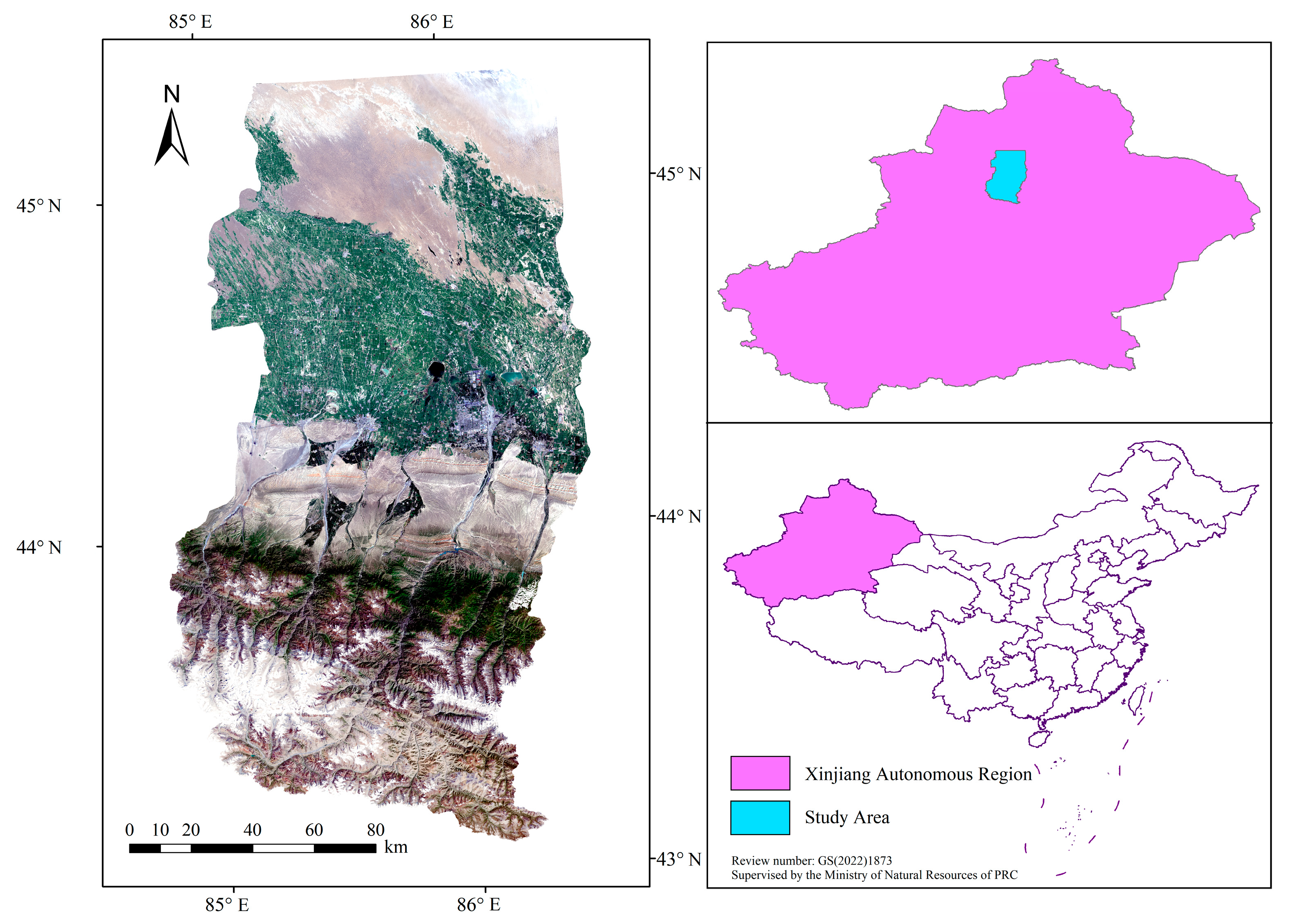
2.1. Study Area

The Manas River Basin is located in northwest China’s Xinjiang Uygur Autonomous Region. The Manas River originates from the northern foot of Mount Ilianhabirga in the Tianshan Mountains and flows toward Manas Lake in the Gurbantunggut Desert (Figure 1). The basin is the core area of the northern slope economic zone of the Tianshan Mountains and the largest oasis agricultural area in Xinjiang [25]. The annual average precipitation is approximately 150–200 mm with an average temperature of 6.8 °C. The interannual temperature difference can reach 80 °C, which is characteristic of a temperate continental climate. The terrain is relatively high in the southern region and relatively low in the northern region with an average altitude of 366–407 m. The sequence of land cover types along the Manas River from southwest to northeast includes alpine snow, alpine meadow, mountain coniferous forest, mountain desert steppe, agricultural oasis, and temperate desert [26]. The vertical zonality is evident, as it is a typical mountain–oasis–desert ecosystem.

The Manas River spans 324 km, with a catchment area of 5156 km² and an average annual runoff of 13.41 × 10⁸ m³, which is sourced mainly from atmospheric precipitation and melting ice and snow [27]. The basin contains multiple inland river systems, including the Tasi River, Manas River, Ningjia River, Jingou River, and Bayin River, which are arranged from east to west. All five rivers originate from Mount Ilianhabirga and converge into Manas Lake from south to north. Administrative divisions within the basin include Shihezi City, Manas County, and Shawan City.

In the 1950s, the Chinese government constructed irrigation systems and implemented cotton and grain cultivation in the Manas River Basin to stabilize and develop the frontier region. Large areas of wasteland have been cultivated into agricultural oases [28]. The social–economic level has experienced rapid development and has become a national-level modern agricultural demonstration zone. Simultaneously, a significant amount of artificial reclamation has resulted in harm to natural ecosystems [29]. Habitat quality is gradually deteriorating, and the sustainable development of the basin is facing challenges.

2.2. Data Sources

① Land use type data

The land use type data utilized China’s 30 m spatial resolution land cover data from 1990 to 2021, which was released by Yang and Huang Xin’s team at Wuhan University [30]. The land use types were reclassified into 9 categories: cultivated land, forestland, shrub land, grassland, water area, snow/ice, bare land, impervious surfaces, and wetland. The land use data were utilized primarily for calculating various landscape pattern indices, ecological footprints, and ecological carrying capacities. The calculations were performed via ArcGIS 10.2 and Fragstats 4.2 software.

② Meteorological data

The temperature and precipitation data utilized China’s 1 km resolution monthly precipitation dataset (1901–2020) released by Peng Shouzhang’s team at the China National Tibetan Plateau Scientific Data Center [31].

Potential evapotranspiration data from the China 1 km monthly potential evapotranspiration dataset (1901–2022) were also utilized. This dataset was calculated via the Hargreaves potential evapotranspiration formula [32].

The meteorological data were used mainly to calculate water yield, carbon sequestration capacity, and ecosystem resilience. The calculation process was completed via ENVI 5.3 and the InVEST water yield model.

③ Soil data

The soil data utilized were from the world soil database constructed by the Food and Agriculture Organization of the United Nations (FAO) and the International Institute for Applied Systems Analysis and were revised on the basis of China’s second national land survey data provided by the Institute of Soil Science, Chinese Academy of Sciences [33,34].

The data used for determining the depth of the root-restricting layer came from the Chinese bedrock depth data published by Fapeng Yan and had a spatial resolution of 100 m [35].

Both bedrock depth data and soil data were used to calculate heterotrophic respiration (Rh).

④ Socioeconomic data

The social and economic data, including industry production value, agricultural output, industrial output, energy consumption structure, water pollution, and local financial data, were collected and compiled via statistical yearbooks by the local statistical departments of Shihezi, Manas, and Shawan. This method was used for calculating the carbon footprint and water footprint.

⑤ Net primary product data

The annual net primary production (NPP) was derived from the sum of all 8-day net photosynthesis (PSN) products (MOD17A2H) from a given year, which were released by NASA and provide information about annual NPP at a 500 m pixel resolution [36]. NPP data were used to calculate the carbon sequestration capacity.

3. Methods

3.1. Constructing the Assessment Indicator System

Regional ecosystems are composite systems in which the natural environment and human activities are closely coupled. The interactions between humans and nature impact various factors, such as material, energy, and landscape patterns, and they are characterized by complexity [37]. The PSR model not only considers resource and ecological elements but also encompasses economic, land use and social development elements. It can better reflect the pressure of human activities on ecosystems and improvements in EH through human responses, which is beneficial for comprehensive and objective assessment of EH conditions [38].

In the PSR model, different elements within the ecosystem interact with each other and are subjected to pressures from the natural environment or human activities. When the “pressure” endured by an ecosystem exceeds its carrying capacity, it will force a change in its “state”. When changes in “state” have a negative impact on human survival and development, humans take measures to respond and reduce the “pressure” on ecosystems. Through this process, EH improves.

This study was based on the conditions and characteristics of the Manas River Basin ecosystem, considering the hierarchy of indicators and the availability of data. An EH assessment indicator system for the study area was constructed from three aspects: pressure, state, and response (

Table 1. Ecosystem health assessment indicator system for the Manas River Basin.

Criterion	Factor	Indicator	Indicator Nature	Weight
Pressure	Land Demand for Ecosystems	Ecological footprint	-	0.083
	Material Demand for Ecosystems	Carbon footprint	-	0.030
		Water footprint	-	0.063
State	The Material Carrying Capacity of Ecosystems	Carbon sequestration	+	0.041
		Water yield	+	0.084
	The Spatial Carrying Capacity of Ecosystems	Ecological carrying capacity	+	0.091
	Stability of Landscape Space Structure	Shannon’s diversity index	+	0.063
		Shannon’s evenness index	+	0.063
		Landscape contagion	+	0.066
		Landscape connectance	+	0.082
Response	Anti-Disturbance Ability of Ecosystems	Ecosystem resilience	+	0.045
		Landscape disturbance degree	-	0.040
	Ecological Management	Forestland expansion	+	0.106
		Construction land expansion	-	0.025
		Environmental protection investment	+	0.118

).

“Pressure” refers to the stress on the natural carrying capacity caused by excessive human demand for resources and the environment. This indicator system measures “pressure” via the carbon footprint, water footprint, and ecological footprint. The carbon footprint and water footprint connect the main production sectors of humanity, spanning from upstream to downstream material production and consumption. They represent the material manifestations of the “pressure” that humans exert on the ecosystem. The ecological footprint reflects the human demand for different land types from a spatial perspective, reflecting the spatial pressure on the ecosystem [39].

“State” refers to the stable condition of the structure and function of an ecosystem. In this study, the water yield, carbon sequestration, ecological carrying capacity, and landscape pattern index are used to assess the “state” of EH. The water yield corresponds to the water footprint, and carbon sequestration corresponds to the carbon footprint, characterizing the extent to which ecosystems can withstand material pressures. The ecological carrying capacity corresponds to the ecological footprint, which reflects the supply of various land types in the ecosystem [40]. The landscape pattern and its changes are a comprehensive reflection of the regional eco-environment system produced by the interaction of natural and human factors. The landscape pattern index can quantitatively reflect the spatial structural characteristics of the landscape as well as the effects of various ecological processes, including disturbances and succession, in the spatial dimensions. Landscape pattern indices, including Shannon’s diversity index (SHDI), Shannon’s evenness index (SHEI), landscape contagion (CONTAG) and landscape connectance (CONNECT), are introduced to represent the spatial structure condition of the ecosystem landscape.

“Response” includes measures taken by humans to address the deterioration of habitat quality and the ability of the ecosystem to restore its own vitality and stability when disturbed by “pressure” [41]. Ecosystem resilience is used to characterize the “response” level of the ecosystem. The expansion of forestland area and investment in environmental protection represent the response of society to environmental degradation.

Indicator weights were determined using the entropy weight method. The entropy weight method is an objective weighting method based on information entropy theory. It determines the weights by calculating the discrete degree of indicator data. The smaller the information entropy of the indicator, the greater its discrete degree, and the higher the weight assigned. This method reduces the influence of subjective factors, as well as exhibits monotonicity and scale independence, making the assessment results more objective.

3.2. CC-PSR Ecosystem Health Assessment Model

3.2.1. CC-PSR Ecosystem Health Index

On the basis of the assessment indicator system designed in the previous section, combined with the coupling coordination model, the ecosystem health index (EHI) of the Manas River Basin was constructed as follows:

$$EHI=\sqrt[3]{(1-P)\times S\times }R$$

(1)

$$P={\displaystyle \sum _{i=1}^n{I}_{pi}\cdot W_{pi}}$$

(2)

$$S={\displaystyle \sum _{i=1}^n{I}_{si}\cdot W_{si}}$$

(3)

$$R={\displaystyle \sum _{i=1}^n{I}_{ri}\cdot W_{ri}}$$

(4)

where EHI represents the ecological health index. P, S, and R are the composite indices of “pressure”, “state”, and “response”, respectively. I_pi, I_si, and I_ri are the standardized values of various “pressure”, “status”, and “response” indicators, respectively. W_i represents the weight of each indicator, which is calculated via the entropy weight method.

The ecosystem, as an organic whole, contains coupled relationships among interrelated elements. These internal correlations and mechanisms affect the stability of EH. Many existing EH evaluation models directly assign weights to various indicators and calculate them, neglecting the degree of coordination and adaptation between indicators. The CC-PSR model combines paired indicators that are interrelated within the indicator system into coupled coordination pairs and calculates the CCD between them. The calculated CCD was incorporated as a coefficient into the calculation of the indicator values to measure the impact of their coordination relationship on EH. Therefore, the calculation formula for the indicator value is as follows:

$$I_a=V_a\times D_{ab}$$

(5)

Or

$$I_a=V_a\times (1-D_{ab})$$

(6)

where I_a represents the value of indicator a, which is related to indicator b. V_a is the measurement of indicator a. D_ab is the coupling coordination coefficient, which represents the coupling coordination degree between indicator a and indicator b.

The CCD in the formula is commonly used to analyze the level of coordinate development. The “coupling degree” refers to the extent of mutual influence and constraints among elements. The degree of coordination refers to the extent of benign coupling in a coupling relationship and reflects the quality of coordination [42,43]. The formula is as follows:

$$D=\sqrt{C\times T}$$

(7)

$$C=\sqrt{{\displaystyle \frac{V_a\times V_b}{{(V_a+V_b)}^2}}}$$

(8)

$$T=\alpha \cdot V_a+\beta \cdot V_b$$

(9)

where D represents the degree of coupling coordination. C is the coupling degree, and T is the composite index. V_a and V_b represent the standardized values of the measurements of two interrelated indicators.

The purpose of this method is to assess whether the internal elements of the ecosystem tend toward stability and order and whether they are in a benign coupling state. Avoiding the isolated calculation of individual indicators and thus neglecting the positive or negative impacts of the correlations between indicators on the overall ecosystem improves the objectivity of the assessment results.

3.2.2. Establishing a Coupling Coordination Coefficient

On the basis of the correlation between different indicators in the indicator system, the following coupling coordination relationship pairs were identified (

Table 2. Coupling coordination relationship pairs.

Ecological footprint—Ecological carrying capacity

Carbon footprint—Carbon sequestration

Water footprint—Water yield

Shannon’s diversity index—Shannon’s evenness index

Landscape contagion index—Landscape connectance index

Ecosystem resilience—Landscape disturbance degree

Forestland expansion—Construction land expansion

Environmental protection investment—Local fiscal expenditure

).

According to the calculation results of the CCD, the natural breaks method was used to divide the CCD into five ranks (

Table 3. Ranks of the degree of coupling coordination.

0 < C ≤ 0.32	0.32 < C ≤ 0.41	0.41 < C ≤ 0.67	0.67 < C ≤ 0.84	0.84 < C ≤ 1
Imbalance	Moderate imbalance	Low coordination	Moderate coordination	Advanced coordination

(Note: The specific division interval is adjusted on the basis of the calculation results of the CCD between different indicators).

). The natural breaks method is based on the natural breaks inherent in a dataset. The boundary values are set at the locations where the differences between data values are comparatively large to divide the data into different ranks. The specific definitions of the five ranks are as follows:

Advanced coordination (0.84 < C ≤ 1): The coordination status between the two indicators is very good. The changing trends of both are highly consistent, complementing each other seamlessly.

Moderate coordination (0.67 < C ≤ 0.84): The coordination status between the two indicators is moderate. The changing trends of both are basically consistent.

Low coordination (0.41 < C ≤ 0.67): At this level, there is limited coupling, and the changing trends of two indicators exhibit some alignment. The degree of mutual compatibility is relatively weak.

Moderate imbalance (0.32 < C ≤ 0.41): The coupling between the two indicators is minimal. The changing trends of both are basically opposite without significant synergy.

Imbalance (0 < C ≤ 0.32): There is no coordination and adaptability between the two indicators. They vary independently, and their interactions are weak.

On the basis of whether the natures of the paired indicators are the same and the calculation results of the CCD, the coupling coordination coefficient was established in the following three scenarios.

Scenario 1: When both the indicator natures of the paired indicators are either positive or negative, regardless of the rank of their CCD, their indicator values are as follows:

$$I_a=V_a\times D_{ab}$$

(10)

$$I_b=V_b\times D_{ab}$$

(11)

I_a and I_b represent the values of two interrelated indicators. V_a and V_b represent the measurements of indicators a and b, respectively. D_ab is the CCD between V_a and V_b.

Scenario 2: When the indicator natures of the paired indicators are different but their CCD is “moderate coordination” or above, their indicator values are as follows:

$$I_a=V_a\times D_{ab}$$

(10)

$$I_b=V_b\times D_{ab}$$

(11)

I_a and I_b represent the values of two interrelated indicators. V_a and V_b represent the measurements of indicators a and b, respectively. D_ab is the CCD between V_a and V_b.

This situation indicates that the pair of indicators with opposite natures has a consistent increasing/decreasing trend during a certain period. These effects counteract each other, thereby not fundamentally impacting regional EH.

Scenario 3: When the indicator natures of the paired indicators are different and their CCD is “low coordination” or below, their indicator values are as follows:

$$I_a=V_a\times (1-D_{ab})$$

(12)

$$I_b=V_b\times D_{ab}$$

(13)

I_a and I_b represent the values of two interrelated indicators. V_a and V_b represent the measurements of indicators a and b, respectively. D_ab is the CCD between V_a and V_b.

This situation indicates that this pair of indicators has opposite trends during a certain period. The impact of both on the EH method is significantly imbalanced. The side with a larger magnitude of change significantly impacts the EH, suppressing the side with a smaller magnitude of change. If the dominant side in this case is a positive indicator, then this imbalance can be considered a “benign imbalance”, implying that positive indicators can effectively counteract the adverse effects of negative indicators. Otherwise, it is a “malignant imbalance”, indicating that negative impacts will drive the severe deterioration of the EH condition.

3.3. Indicator Calculation

Each indicator was calculated sequentially according to the CC-PSR model and the designed indicator system. The formulas and interpretations are presented in the table below (

Table 4. Indicator formulas and calculations.

Indicator	Formula	Calculation Instructions	Variable Descriptions	Source of Coefficient
Carbon footprint	$E_i=P_i\cdot F_i$	The carbon footprint calculation relied on the coefficient method. The annual greenhouse gas emissions from industrial, agricultural, energy, transportation, and citizen life were calculated for both upstream production and downstream consumption.	Ei represents the greenhouse gas emissions of the i-th category products or services (t•CO2-eq). Pi represents the supply quantity for the i-th category of product or service. Fi represents the greenhouse gas emission factor for the i-th category of products/services.	[44]
Water footprint	${WF}_{total}={WF}_{blue}+{WF}_{green}+{WF}_{grey}$	Water footprint refers to the amount of water resources required for all products and services consumed in a region. This study calculated the blue water footprint, green water footprint, and gray water footprint of various industries based on the “Water Footprint Assessment Manual”	WFtotal represents the total water footprint of the region. WFblue, WFgreen, and WFgrey represent blue water footprint, green water footprint, and gray water footprint, respectively. All units are in m3.	[45,46,47,48,49]
Ecological footprint	$EF=N\times ef=N\times {\displaystyle \sum _{i=1}^n{\lambda }_i\cdot {aa}_i}=N\times {\displaystyle \sum _{i=1}^n{\lambda }_i\cdot \frac{c_i}{k_i}}$	To measure the sustainable utilization of land resources, the total demand for various productive lands by the regional population was calculated through the ecological footprint method.	EF represents the ecological footprint (hm2). N represents the population. ef represent the per capita ecological footprint (hm2/person). λi represents the equilibrium factor of the i-th type of land. aai is the area of the i-th type of biological productive land per capita (hm2/person). ci is the annual per capita production of the i-th type of consumer goods. ki represents the annual production of the i-th category of consumer goods in the region.	[50,51,52]
Carbon sequestration	$NEP=NPP-Rh$ $Rh=0.4679\times Rs+114.42$ $\begin{array}{l}Rs=(0.588+0.118\times SOC)\times e^{\ln (1.83\times e^{-0.006\times T})\times T÷10}\\ \times (P+2.972)÷(P+5.657)\end{array}$	Without considering other factors, carbon sequestration can be represented by net ecosystem productivity (NEP) [53,54], and it was calculated using the equation NEP = NPP − Rh.	NEP represents the annual net ecosystem productivity (t/yr). NPP represents the annual net primary production (t/yr). Rh is theannual soil heterotrophic respiration (t/yr), and Rs is the annual soil respiration (t/yr). T and P represent temperature (°C) and precipitation (mm), respectively.	[55]
Water yield	$Y(x)=\left[1-{\displaystyle \frac{AET(x)}{P(x)}}\right]\cdot P(x)$	According to the principle of water balance, the annual water yield was calculated by subtracting actual evapotranspiration (including land surface evapotranspiration and vegetation transpiration) from precipitation at the scale of grid [56].	Y(x) represents the annual water yield (m3) of grid x. AET(x) is the annual actual evapotranspiration (m3) of grid x, and P(x) is the annual precipitation (m3) of the grid.
Ecological carrying capacity	$EC=N\times ec=N\times {\displaystyle \sum _{i=1}^n{a}_i·r_i·y_i}$	Ecological carrying capacity is the ability of the natural environment to provide various types of ecological capital for the local population [50]. The ecological carrying capacity was determined by calculating the unit yield of each category of biological productive land.	EC represents the ecological carrying capacity (hm2). N represents the population. ec is the per capita ecological carrying capacity (hm2/person). The ai is the area of the i-th type of biological productive land per capita (hm2/person). yi is the yield factor for the i-th type of biological productive land.	[57]
Shannon’s diversity index	$SHDI=-{\displaystyle \sum _{i=1}^n(P_i\times \ln P_i)}$	Landscape diversity refers to the diversity of landscape units in terms of structure and function, which reflects the complexity of regional landscapes. Landscape diversity has a significant impact on the material cycling, energy flow, as well as species migration and habitat within a region [58]. The method used to calculate landscape diversity was the Shannon Landscape Diversity Index (SHDI). The larger the value is, the more abundant the landscape patch types per unit area in the region.	SHDI is the Shannon Landscape Diversity Index (value range greater than 0). Pi represents the proportion of the landscape occupied by patch type i.
Shannon’s evenness index	$SHEI={\displaystyle \frac{-{\displaystyle \sum _{i=1}^n(P_i\cdot \ln P_i)}}{\ln n}}$	Landscape evenness describes the degree of uniformity in the spatial distribution of different landscape types and was calculated using Shannon’s Landscape Evenness Index (SHEI). A higher value indicates a more uniform distribution of various landscape patches [59]. Good landscape diversity and evenness are beneficial for maintaining the stability of ecological space.	SHEI is the Shannon Landscape Diversity Index (0 ≤ SHEI ≤ 1). Pi represents the proportion of the landscape occupied by patch type i. n represents the number of patch types present in the landscape.
Contagion index	$CONTAG=\left[1+{\displaystyle \sum _{i=1}^n{\displaystyle \sum _{j=1}^n\frac{P(i,j)\cdot \log (P(i,j))}{2\cdot \log (n)}}}\right]\times 100\%$	The Contagion Index measures the degree of clumping and dispersion in landscape distribution. The higher the CONTAG index is, the higher the degree of aggregation of landscape patches. Conversely, when the CONTAG index is lower, the landscape patches are more disaggregated [59].	CONTAG represents the Contagion Index, which is measured in percentage. P(i,j) represents the probability that patch types i and j are adjacent. n represents the number of patch types present in the landscape.
Connectance index	$CONNECT={\displaystyle \frac{{\displaystyle \sum _{i=1}^m{\displaystyle \sum _{j=j}^n{c}_{ijk}}}}{{\displaystyle \sum _{i=1}^m\frac{n_i·(n_i-1)}{2}}}}$	Connectance index measures the degree of connectivity between landscape patches [60]. It assesses the organic connections between landscape elements in space, ecological processes, and ecological functions. Good landscape connectivity is beneficial for maintaining ecological corridors, which allow for the diffusion and exchange of species [58].	CONNECT represents the Contagion Index in percent. cijk represents the connection between patch j and k of the corresponding patch type i. ni represents the number of patches in the landscape of the corresponding patch type.
Landscape disturbance	$\begin{array}{c}LD=PD\cdot w_1+DIV\cdot w_2+SPL\cdot w_3\\ PD={\displaystyle \frac{N}{A}}\hspace{1em}DIV=\left[1-{\displaystyle \sum _{i=1}^n{(\frac{a_{ij}}{A})}^2}\right]\hspace{1em}SPL={\displaystyle \frac{A}{{\displaystyle \sum _{i=1}^m{\displaystyle \sum _{j=1}^n{a}_{ij}}}}}\end{array}$	Landscape disturbance is based on the principles of landscape ecology, weighting and summing the landscape fragmentation, landscape division and patch density to reflect the disturbances experienced by the landscape [61].	LD represents landscape disturbance degree. PD, DIV, and SPL, respectively represent patch density, landscape division and landscape fragmentation. w1, w2, and w3 are the weights of PD, DIV, and SPL, with values of 0.3, 0.5, and 0.2, respectively.
Ecosystem resilience	$\begin{array}{c}ER=\epsilon ·\mu ·{ECO}_{res}\\ {ECO}_{res}=H{\displaystyle \sum _{i=1}^n{S}_i\cdot P_i}\\ \mu ={\displaystyle \frac{H\cdot V}{c_1\cdot c_2}}\end{array}$	Ecosystem resilience refers to the ability of an ecosystem to maintain its original state after being impacted by an external disturbance [62]. It mainly includes two aspects: the ecosystem resilience strength and resilience [63].	ER is ecosystem resilience. ε is the adjustment coefficient (the value is 0.01 according to reference). μ is the resilience strength coefficient of the ecosystem. ECOres is the ecological system resilience limit. H is the landscape diversity index. V is the vegetation index. C1 is the annual precipitation change rate, C2 is the annual temperature change rate. Si is the resilience score of land type i. Pi is the proportion of land type i.

):

4. Results and Analysis

4.1. Ecosystem Health Conditions

On the basis of the assessment indicator system established in the previous section, the ecological health index (EHI) of the Manas River Basin from 2000 to 2020 was calculated via the CC-PSR model. Using the natural breakpoint method, the results were divided into four levels: “healthy” (EHI > 0.29), “subhealthy” (0.25 < EHI ≤ 0.29), unhealthy (0.2 < EH ≤ 0.25) and “diseased” (EHI < 0.2).

From the calculation results, the EH conditions calculated by both the conventional PSR model and CC-PSR model showed an increasing trend over the past 21 years (Figure 2a). Both showed significant peaks in 2013 and 2016. However, compared with the conventional PSR model, the CC-PSR model reflects a relatively smooth fluctuation in the EH in the first 11 years. After 2012, the fluctuation of the EH significantly increased. The CC-PSR model can more clearly reflect the inflection point of EH changes.

Overall, the EHI of the Manas Basin has fluctuated and increased over the past 21 years. In the early years (2000–2006), the growth was relatively slow and remained in an “unhealthy” condition for a long period. The lowest EHI value over 20 years occurred in 2000, at 0.186. Between 2006 and 2008, it remained in a “subhealthy” condition. After 2009, the EH condition continued to improve, reaching a peak of 0.385 in 2013. Although there were some fluctuations in the following seven years, the EH condition remained within the “healthy” range for many years with the average EHI maintained at 0.35.

The three dimensions of “pressure”, “state”, and “response” were analyzed. From 2000 to 2006, the Manas River Basin had low “pressure” but was limited by low levels of “response” and “state”, and the EHI during this period remained low for a long period. Owing to the lack of planned land reclamation and overgrazing, desertification and salinization problems frequently occur [22]. This situation caused an unstable “state” of the ecosystem, with increasing “pressure” levels, and the EHI began to decline in 2007. From 2008 to 2013, under the development plan of “urban agriculture integration” and “rapid industrialization”, the level of industrialization and agricultural modernization in the Manas River Basin rapidly improved [64]. This led to a continuous increase in “pressure” on the ecosystem, which reached 0.132, the highest level in 21 years.

To cope with ecological pressure, since 2008, regional governments have actively implemented precision fertilization and water and fertilizer synchronization irrigation in agriculture. In industry, efforts have been made to increase energy efficiency and control pollution in the heavy chemical industry and the textile printing and dyeing industry [65,66]. In terms of ecological governance, local governments have effectively managed soil salinization on agricultural land and have actively engaged in windbreak and sand fixation efforts. Mechanized afforestation has been carried out in the northern part of the oasis, and shelterbelts have been constructed. In 2011, local standardized water-saving irrigation projects and returning farmland to forest programs achieved good results. Under the combined effects of various factors, the “response” level significantly increased, rising from 0.07 in 2009 to 0.22 in 2013 (Figure 2c). In the following three years (2014–2016), the “state” level also rose to a peak of 0.4 and continued to remain above 0.3. Under the combined effects, the EH condition gradually transitioned from “subhealthy” to “healthy” between 2013 and 2016. These results indicate that human response measures can effectively improve the “state” of the ecosystem and enhance overall EH. However, the implementation of the “response” has a certain lag.

From 2015 to 2020, many intense cotton and grain processing enterprises with high energy consumption and high emissions were rectified or closed, leading to a slight increase in the “response” level during this period, which was maintained at a relatively good value of 0.155. The “state” level consistently remained above 0.26, which is historically high, thus maintaining good EH. The EH index fluctuated within the range of 0.335 to 0.381, which is considered a “healthy” level.

4.2. Regional Carbon Footprint, Water Footprint, Ecological Footprint, and Corresponding Carrying Capacity

During the study period, the carbon footprint—carbon sequestration, water footprint—water yield, and ecological footprint—ecological carrying capacity in the Manas River Basin each exhibited distinct variation tendencies.

The carbon footprint change tendency exhibited an inverted U-shaped pattern, initially increasing and then decreasing (Figure 3a). In the initial 14 years, carbon emissions experienced a period of accelerating increase. During this period, there was a rapid development of light industries such as cotton spinning and the intense processing of pastoral products, which was driven by the intensification of agriculture and agro-industrial integration. Some fertilizer producers and agricultural equipment companies also established factories in Manas County and Shihezi city for production. Greenhouse gas emissions progressively rose annually, culminating in a peak of 37.78 million tons in 2014. During the “13th Five-Year Plan” period (2016–2020), land use control was systematically enforced in accordance with the national policy of “Three Red Lines” (ecological protection red line, permanent basic farmland, and urban development boundary) for national land space [66,67]. Water consumption and carbon emissions in the Manas River Basin began to decrease simultaneously in 2015. By 2020, the annual greenhouse gas emissions had decreased to 25.77 million tons. In terms of the carbon emissions structure, industrial and agricultural production accounted for 57% and 28%, respectively, and they are the main sources of regional carbon emissions. Carbon emissions from daily living and transportation contributed only 4%.

Constrained by precipitation and vegetation levels, the regional carbon sequestration capacity has remained low for many years without significant improvement (Figure 3a). The maximum annual carbon sequestration is only 68.76 million tons (2016). Regarding carbon emissions, it can be concluded that the Manas River Basin has been a large carbon source for an extended period. The CCD between carbon emissions and carbon sequestration has been in an “imbalanced” condition. The carbon sequestration of ecosystems has never been able to effectively offset regional carbon emissions, causing immense pressure on EH.

The water footprint calculation results reveal that the trend of regional water consumption changes is similar to the trend of carbon emissions. In early years (2000–2011), agriculture in the region focused primarily on cotton, fruit, and vegetable cultivation. The irrigation methods were relatively crude and lacked effective recycling measures for water resources and water-saving facilities. The development of mechanized agriculture and the expansion of local industrial and mining enterprises greatly increased water consumption. From 2000 to 2011, the regional annual water footprint increased rapidly from 40,660 to 231,860 m³ (Figure 3b). Since 2013, local governments have imposed restrictions on the total amount of water resource utilization and water use efficiency. By optimizing agricultural production processes, promoting water-saving transformation in irrigation areas, and popularizing drip irrigation technology, the accelerating trend of water resource consumption was effectively slowed [68]. The total water footprint of the basin reached a peak of 2.93 billion m³ in 2015 and began to decline the following year. It gradually decreased over the next 5 years to 1.627 billion m³ in 2020.

The average annual water yield in the Manas River Basin was 1.3 billion m³ over 21 years, but there was significant interannual variability. Owing to the cyclical changes in climate, the water yield in most years fluctuated within the range of 980 to 1.54 billion m³. In years with high precipitation, the extreme annual water yield can reach 2.2 billion m³. The CCD between water yield and the water footprint consistently oscillated between “moderate imbalance” and “low coordination”. In the early years (2000–2007), the water yield capacity was essentially sufficient to meet the growing water demand for production and construction activities in the region. Given that the water yield exceeded the water footprint during this period, the “moderate imbalance” between them can be considered a benign imbalance, indicating that water consumption was still within the water resources carrying capacity (Figure 3c). In the middle term (2007–2015), with the increase in water consumption in industry and agriculture, the water yield struggled to meet the development demand of the region. According to statistics from the “Xinjiang Water Resources Bulletin”, during this period, the Manas River, Tasi River, and Bayin River in the Manas River Basin experienced varying degrees of water level decline [69]. The gradually increasing water consumption exceeded the water yield, and the CCD between them fluctuated around the cyclical variation in water yield. “Moderate imbalance”, which was a malignant imbalance, often occurred. In the later period (2015–2020), with the completion and operation of the Kenswatt Water Conservancy Hub in 2016, the seasonal water shortage in the region was alleviated, and agricultural water consumption also significantly decreased [70]. The CCD briefly recovered to the “low coordination” level. However, owing to the persistent lack of significant improvement in the regional water yield capacity, the mismatch between the water footprint and water yield still imposes a heavy burden on the “state” of EH.

Over the past 21 years, the overall changes in the ecological footprint and ecological carrying capacity have been relatively small. The ecological footprint has undergone minor fluctuations during this time period (Figure 3b). The minimum value was recorded in 2000 at 2.05 million square meters, whereas the maximum value was observed in 2010 at 2.12 million square meters. At the end of the study period, the value had decreased to 2.1 million square meters. In terms of proportion, the grassland ecological footprint in the Manas River Basin has the highest proportion, representing 48% of the total ecological footprint. Grasslands play crucial roles in soil and water conservation in arid regions. A high ecological footprint of grasslands indicates the presence of overgrazing, which poses risks of grassland degradation and desertification. The ecological footprint of cultivated land in the Manas River Basin steadily expanded, reflecting an increasing demand for agricultural land in this region as an agricultural oasis. The ecological footprints of forestland, desert, and water areas were low, representing 11%, 7%, and 12% of the total, respectively. In terms of the ecological carrying capacity, the regional ecological carrying capacity has slowly increased over the past 21 years, experiencing only a minor decrease between 2012 and 2015. The minimum value was 1.52 million square meters in 2000, and the maximum value was 1.63 million square meters in 2011. From the perspective of the composition of the ecological carrying capacity, grassland and cultivated land presented the highest ecological carrying capacities, accounting for 45% and 32%, respectively. With the promotion of precision agriculture and water-saving irrigation by local agricultural departments, the carrying capacity of cultivated land steadily increased. Second, the ecological carrying capacity of forestland and water areas consistently remained stable due to their low population density, at 11% and 9%, respectively. The CCD between the ecological footprint and the ecological carrying capacity exhibited a limited range of variation, consistently falling within the spectrum of “moderate coordination” to “low coordination”. On the basis of the aforementioned analysis, the carrying capacity of key land types such as cultivated land, forestland, and wetlands in the region can effectively adapt to the ecological footprint. In conjunction with the implementation of the “Grain for Grass” project starting in 2008 and the grazing restrictions issued in 2011, the coordinated development of the ecological carrying capacity and ecological footprint in the Manas River Basin has been ensured.

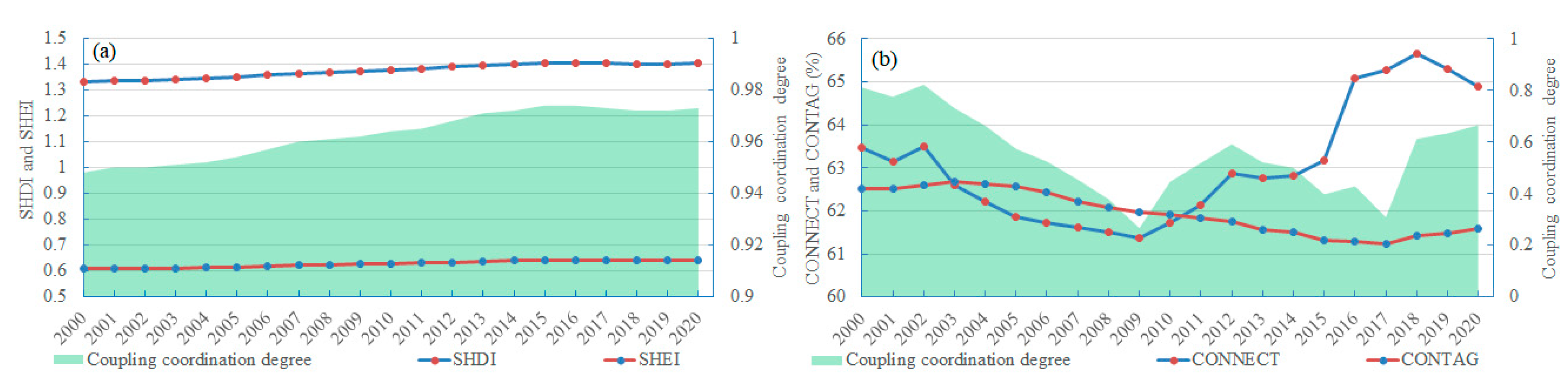
4.3. Landscape Pattern Analysis

Over the course of 21 years, the landscape pattern of the region consistently remained in relatively good condition.

According to the calculation results, the SHDI and SHEI did not change significantly (Figure 4a). The SHDI slightly increased by 5.53% over 21 years, whereas the SHEI increased by only 5.54%. The CCD between the two remained above 0.945 without a significant decline. This situation reflects that the regional landscape diversity is in good condition, and is maintaining stable landscape heterogeneity. However, the SHEI level was low for a long time, indicating that the dominant landscape types (desert, grassland) in the region are concentrated and contiguous.

CONNECT first decreased but then increased over the course of 21 years, showing substantial variation (Figure 4b). In early years, against the backdrop of Western development, Shawan City, Shihezi City, and Manas County entered a rapid urbanization phase. The expansion of construction and cultivated land lacked rational planning, leading to sprawling anthropogenic land cover and resulting in the fragmentation of landscape patterns. During the first decade, CONNECT consistently declined and reached its lowest point of 61.38% in 2009. Following the introduction of the “Development Plan for the Northern Slope Economic Zone of the Tianshan Mountains” in 2011, land use within the basin became more intensive and consolidated. The CONNECT level steadily increased during this period and reached its peak of 65.65% in 2018. In contrast, CONTAG continuously declined over the past 21 years with an average value of approximately 61.5%. This situation indicated an agglomeration trend of multiple landscape types within the region. The CCD between CONNECT and CONTAG was dominated by CONNECT, and the trend of changes was similar to that of CONNECT. In both the early stage (2000–2002) and the later stage (2016–2020) of the study, a high degree of coordination was maintained, indicating that most of the landscape patches within the region had maintained good spatial continuity and that the degree of landscape fragmentation was not high. Various types of landscape patches maintained connections in spatial structure and ecological functions, which is conducive to the circulation of material, energy, and information in the ecosystem. This connectivity also increases the likelihood of wildlife corridors [71].

The integration of the four landscape pattern indices revealed that a well-maintained landscape ecological pattern contributed to the stability of the eco-spatial structure in the Manas River Basin. This stability is an important foundation for maintaining the ‘state’ in the ecosystem. The land cover changes caused by human activities have not destroyed landscape diversity or caused severe landscape fragmentation. The increase in landscape connectivity over the last decade has effectively promoted improvements in the “state” of the ecosystem.

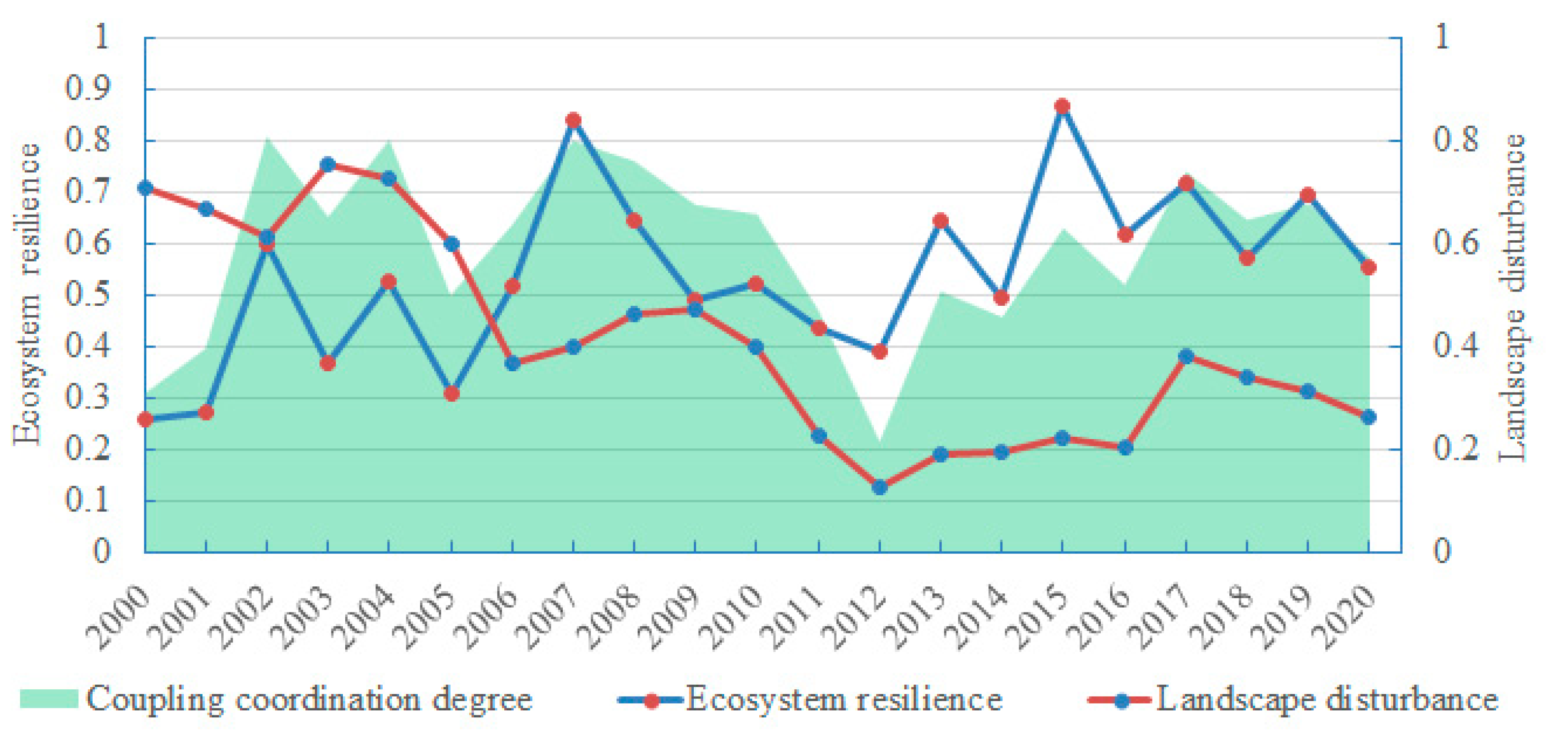
4.4. Ecosystem Resilience and Landscape Disturbances

Over the past twenty years, the level of landscape disturbance has gradually decreased, whereas ecosystem resilience has fluctuated upward (Figure 5). Before 2005, the level of landscape disturbance was greater than that of ecosystem resilience. Afterward, with vegetation restoration and the implementation of the ecological protection policies mentioned earlier, landscape disturbance began to decrease significantly. In 2012, it decreased to a minimum of 0.127. Although it increased slightly afterward, it generally remained at a relatively low range of 0.18–0.34. In the early years, the level of ecosystem resilience was low at 0.26, but it maintained an increasing trend. After peaking at 0.84 in 2007, it then declined somewhat. After 2012, it fluctuated repeatedly, at approximately 0.61. Fluctuations in ecosystem resilience may also have been caused by cyclical changes in climate and precipitation.

The coupling coordination between ecosystem resilience and landscape disturbance lacks stability. The maximum value of ecological resilience determines the upper limit of the CCD, whereas the minimum value of landscape disturbance determines the lower limit of the CCD. Overall, increasing ecosystem resilience and decreasing landscape disturbance are beneficial for EH.

5. Discussion

A review of the literature reveals that no study has adequately considered the potential impact of the coordinated relationship between interrelated indicators on EH. We introduced the concept of the coupling coordination coefficient for measuring the impact of adaptability and coordination between interrelated indicators on regional EH, improving the conventional PSR model. The CC-PSR model has demonstrated good applicability in assessing the EH of the Manas River Basin. In the design of the assessment indicator system, previous studies have tended to select indicators related to pollution, biological communities, and ecosystem productivity [72,73]. This paper innovatively uses indicators such as carbon footprint, water footprint, ecological footprint, and landscape pattern index. These contribute to the comprehensive analysis and understanding of the health and change processes of composite ecosystems with a closely coupled man–land relationship.

Although the overall EH of the Manas River has shown a positive upward trend, there are still significant interannual fluctuations, indicating that EH remains unstable. The impact of human activities on EH is significant and far-reaching. Oasis agriculture is an important driving force for the development of the Manas River Basin. However, the Manas River Basin is located in a northwestern arid region with sparse vegetation and scarce water resources, which renders the ecosystem relatively fragile [74]. Years of agricultural operations and agro-industrial production have generated substantial carbon footprints, water footprints, and ecological footprints, exerting immense pressure on ecosystems. The current integrated development model of agriculture and industry is approaching the ecological carrying capacity limit in the Manas River Basin. Arbitrarily expanding the production of cash crops such as cotton and fruit is unsustainable. On the other hand, agricultural production has optimized land use structure and improved landscape patterns, thereby consolidating the EH “state”. Oasis shelterbelts, crops, and other artificial vegetation have increased the NDVI, playing a positive role in enhancing ecosystem resilience. Therefore, viewing the impact of human activities on EH dialectically helps to understand the delicate balance between humans and nature, thereby making reasonable decisions. Fortunately, both the carbon footprint and water footprint declined by the end of the research period. The key to alleviating EH pressure in the future lies in how to balance the supply and demand relationship between agricultural water use and water yield, promote industrial transformation, and achieve carbon emission reduction. Moreover, the findings of this study have shown that enhancing the level of “response” can have a substantial positive impact on EH. The improvement in the “response” has been quite limited in the last two decades, leaving ample space for further advancements. In the future, regional management departments should increase investments in environmental protection in line with the policies of ecological civilization construction and the “Three Red Lines”.

From the carbon footprint calculation results, it can be concluded that carbon emissions in the Manas River Basin peaked in 2014 and have been steadily declining. In the context of China’s carbon neutrality strategy, this contributes to Xinjiang region achieving its carbon peaking goal before 2030 [75,76]. Based on the practice of achieving carbon peaking and carbon neutrality goals in China, strengthening the management and protection of forest and grassland resources, enhancing wetland carbon sequestration capacity, and unleashing agricultural carbon sequestration potential are not only beneficial for improving regional carbon sink but also lead to eco-environmental quality enhancement, thereby improving EH.

This paper has certain limitations. Owing to the limited availability of data, the design of the indicator system did not incorporate factors such as environmental pollution and biodiversity. This inevitably undermines the objectivity of the assessment results. The process of identifying the coupling coordination relationship pairs was subjective and lacks theoretical and methodological basis. All of these leave room for further optimization. In subsequent research, we will optimize the assessment indicator system and analyze the spatial distribution of EH in the Manas River Basin. We will also attempt to explore the potential trade-offs between different indicator elements.

6. Conclusions

This paper constructs the CC-PSR model. By designing a medium-scale regional EH assessment framework that connects natural ecosystems with socioeconomic systems, a quantitative assessment of EH in the Manas River Basin was conducted. Preliminary findings revealed EH defects in the Manas River Basin.

(1) EH has exhibited a fluctuating upward trend over the past 21 years. Compared with the traditional PSR model, the improved CC-PSR model can reflect more EH inflection points. It can more sensitively reflect the fluctuations in the EH caused by changes in pressure, state, or response.

(2) “Pressure” was the primary factor that restricted the improvement in EH conditions during the early period (2000–2009). Influenced by the continuously increasing intensity of human activities, “pressure” originated primarily from the expansion of cotton and grain agriculture in oases and the development of agricultural product processing industries. The changing trend of “pressure” aligned with the variations in the carbon, water, and ecological footprints.

(3) A good landscape pattern and ecological carrying capacity are essential for consolidating the EH “status”. Both the increase in ecosystem resilience and the construction of protective forests positively affect the level of “response”. An improvement in the “response” level can drive the growth of the “state” and alleviate “pressure”, thus substantially enhancing the EH condition. However, the utility of “response” significantly lags. Typically, a noticeable enhancement in the EH condition occurs only two years after the “response” level has risen.

(4) The fluctuations in the EHI during the 21-year upward trend originated from cyclical changes in regional water yield and carbon sequestration. This situation may be related to interannual climate variability, as suggested by temperature and precipitation data. Owing to the arid climate and sparse vegetation in this region, the low carbon sequestration capacity and limited water yield represent vulnerabilities to EH.

Although EH conditions have continuously improved over the past 21 years, the EHI is still less than 0.4, and the ecological environment in the Manas River Basin remains very fragile. In the future, leveraging the light and heat advantages of the basin and utilizing water resources efficiently to improve vegetation coverage and the ecological carrying capacity will be crucial for consolidating and enhancing the EH.

References

1. Tilman, D.; Knops, J.; Wedin, D.; Reich, P.; Ritchie, M.; Siemann, E. The influence of functional diversity and composition on ecosystem processes. Science 1997, 277, 1300–1302. [Google Scholar] [CrossRef]
2. Coleman, D.C.; Hendrix, P.F.; Odum, E.P. Ecosystem health: An overview. Soil Chem. Ecosyst. Health 1998, 52, 1–20. [Google Scholar] [CrossRef]
3. World Health Organization. Constitution of the World Health Organization; World Health Organization: New York, NY, USA, 1995; p. 1. [Google Scholar]
4. Costanza, R.; Norton, B.G.; Haskell, B.D. Ecosystem health: New goals for environmental management. In Proceedings of the 1st International Symposium on Ecosystem Health and Medicine, Ottawa, ON, Canada, 19–22 June 1994. [Google Scholar]
5. Rapport, D.J. Evaluating ecosystem health. J. Aquat. Ecosyst. Stress Recovery 1992, 1, 15–24. [Google Scholar] [CrossRef]
6. Lu, Y.L.; Wang, R.S.; Zhang, Y.Q.; Su, H.Q.; Wang, P.; Alan, J.; Rober, C.F.; Mark, B.; Geoff, S. Ecosystem health towards sustainability. Ecosyst. Health Sustain. 2015, 1, 1–15. [Google Scholar] [CrossRef]
7. Yi, C.X.; Nathan, J. A review of measuring ecosystem resilience to disturbance. Environ. Res. Lett. 2021, 16, 053008. [Google Scholar] [CrossRef]
8. Lundberg, J.; Moberg, F. Mobile link organisms and ecosystem functioning: Implications for ecosystem resilience and management. Ecosystems 2003, 6, 0087–0098. [Google Scholar] [CrossRef]
9. Wilcox, B.A. Ecosystem health in practice: Emerging areas of application in environment and human health. Ecosyst. Health 2001, 7, 317–325. [Google Scholar] [CrossRef]
10. Costanza, R. Ecosystem health and ecological engineering. Ecol. Eng. 2012, 45, 24–29. [Google Scholar] [CrossRef]
11. Rapport, D.J.; Costanza, R.; McMichael, A.J. Assessing ecosystem health. Trends Ecol. Evol. 1998, 13, 397–402. [Google Scholar] [CrossRef]
12. Mallick, J.; AlQadhi, S.; Talukdar, S.; Pradhan, B.; Bindajam, A.A.; Islam, A.R.M.T.; Dajam, A.S. A novel technique for modeling ecosystem health condition: A case study in Saudi Arabia. Remote Sens. 2021, 13, 2632. [Google Scholar] [CrossRef]
13. Rong, H.; Huang, X.T.; Ye, X.Y.; Pan, Z.; Wang, H.; Luo, B.; Liu, D.M.; Hu, X.X. County Ecosystem Health Assessment Based on the VORS Model: A Case Study of 183 Counties in Sichuan Province, China. Sustainability 2022, 14, 11565. [Google Scholar] [CrossRef]
14. Rapport, D.J.; Singh, A. An EcoHealth-based framework for State of Environment Reporting. Ecol. Indic. 2006, 6, 409–428. [Google Scholar] [CrossRef]
15. Harwell, M.A.; Gentile, J.H.; McKinney, L.D.; Tunnell Jr, J.W.; Dennison, W.C.; Kelsey, R.H.; Tunnell, J. Conceptual Framework for Assessing Ecosystem Health. Integr. Environ. Assess. Manag. 2019, 15, 544–564. [Google Scholar] [CrossRef] [PubMed]
16. Ashraf, A.; Haroon, M.A.; Ahmad, S.; Abowarda, A.S.; Wei, C.; Liu, X. Use of remote sensing-based pressure-state-response framework for the spatial ecosystem health assessment in Langfang, China. Environ. Sci. Pollut. Res. 2023, 30, 89395–89414. [Google Scholar] [CrossRef]
17. Kashif, I.; Mehebub, S.; Joe, R.; Gopala, A.; Ouseen, G.; Sudha, D.; Archana, C.; Haroon, S. A sustainable solution to manage ecosystem health of wetlands in urban and peri-urban areas of Lucknow district, India using geospatial techniques and community based pragmatic approach. J. Cleaner Prod. 2023, 414, 137646. [Google Scholar] [CrossRef]
18. Zou, S.; Qian, J.; Xu, B.; Tu, Z.; Zhang, W.; Ma, X.; Liang, Y. Spatiotemporal changes of ecosystem health and their driving mechanisms in alpine regions on the northeastern Tibetan Plateau. Ecol. Indic. 2022, 143, 109396. [Google Scholar] [CrossRef]
19. Yi, Q.; Zhang, Y.; Ding, M. Assessment of Urban Ecosystem Health Based on Information Entropy Method. J. Nanning Norm. Univ. (Natual Sci. Ed.) 2021, 38, 122–128. (In Chinese) [Google Scholar]
20. Full Text of Xi Jinping’s Report at 19th CPC National Congress. Available online: http://www.china.org.cn/chinese/2017-11/06/content_41852215.htm (accessed on 21 June 2024).
21. Ge, Q.S.; Fang, C.L.; Jiang, D. Geographical missions and coupling ways between human and nature for the Beautiful China Initiative. Acta Geogr. Sin. 2020, 75, 1109–1119. (In Chinese) [Google Scholar]
22. Wei, H.J.; Xu, Z.H.; Liu, H.M.; Ren, J.H.; Fan, W.G.; Lu, N.C.; Dong, X.B. Evaluation on dynamic change and interrelations of ecosystem services in a typical mountain-oasis-desert region. Ecol. Indic. 2018, 93, 917–929. [Google Scholar] [CrossRef]
23. Liu, R.R.; Dong, X.B.; Wang, X.C.; Zhang, P.; Liu, M.X.; Zhang, Y. Study on the relationship among the urbanization process, ecosystem services and human well-being in an arid region in the context of carbon flow: Taking the Manas river basin as an example. Ecol. Indic. 2018, 132, 108248. [Google Scholar] [CrossRef]
24. Kang, Z.W. Research on Ecosystem Service Function of Manas River Basin Based on InVEST Model. Master’s Thesis, Shihezi University, Shihezi, China, 2022. (In Chinese). [Google Scholar]
25. Xu, S.N.; Yang, J.C.; Li, Y.L. Fluctuations of discharge rate of Manas River and its response to climatic changes during the recently 50 years. Geogr. Geo-Inf. Sci. 2004, 20, 65–68. (In Chinese) [Google Scholar]
26. Feng, Y.X.; Luo, G.P.; Lu, L.; Zhou, D.C.; Han, Q.F.; Xu, W.Q.; Yin, C.Y.; Zhu, L.; Dai, L.; Li, Y.Z.; et al. Effects of land use change on landscape pattern of the Manas River watershed in Xinjiang, China. Environ. Earth Sci. 2011, 64, 2067–2077. [Google Scholar] [CrossRef]
27. Xu, Z.; Fan, W.; Wei, H.; Zhang, P.; Ren, J.; Gao, Z.; Ulgiati, S.; Kong, W.; Dong, X. Evaluation and simulation of the impact of land use change on ecosystem services based on a carbon flow model: A case study of the Manas River Basin of Xinjiang, China. Sci. Total Environ. 2019, 652, 117–133. [Google Scholar] [CrossRef]
28. Xu, Z.; Wei, H.; Fan, W.; Wang, X.; Zhang, P.; Ren, J.; Lu, N.; Gao, Z.; Dong, X.; Kong, W. Relationships between ecosystem services and human well-being changes based on carbon flow—A case study of the Manas River Basin, Xinjiang, China. Ecosyst. Serv. 2019, 37, 100934. [Google Scholar] [CrossRef]
29. Zhao, X.M.; Feng, B. Problems and Development Ideas in the Construction of Modern Agricultural Demonstration Zones: A Case Study of Beiquan Town. Xinjiang Agric. Reclam. Technol. 2012, 35, 51–53. (In Chinese) [Google Scholar]
30. Yang, J.; Huang, X. The 30 m annual land cover dataset and its dynamics in China from 1990 to 2019. Earth Syst. Sci. Data Discuss. 2021, 13, 3907–3925. [Google Scholar] [CrossRef]
31. Peng, S.; Ding, Y.; Liu, W.; Li, Z. 1 km monthly temperature and precipitation dataset for China from 1901 to 2017. Earth Syst. Sci. Data 2019, 11, 1931–1946. [Google Scholar] [CrossRef]
32. Peng, S. 1-km Monthly Potential Evapotranspiration Dataset in China (1990–2021); National Tibetan Plateau Data Center: Beijing, China, 2022. [Google Scholar] [CrossRef]
33. Nachtergaele, F.; van Velthuizen, H.; Verelst, L.; Wiberg, D.; Henry, M.; Chiozza, F.; Yigini, Y.; Aksoy, E.; Batjes, N.; Boateng, E.; et al. Harmonized World Soil Database Version 2.0; FAO; International Institute for Applied Systems Analysis (IIASA): Laxenburg, Austria, 2023; ISBN 978-92-5-137499-3. [Google Scholar] [CrossRef]
34. Shi, J.; Song, G. Soil Type Database of China: A nationwide soil dataset based on the Second National Soil Survey. China Sci. Data 2016, 1, 33. [Google Scholar] [CrossRef]
35. Yan, F.; Wei, S.; Zhang, J.; Hu, B. Depth-to-bedrock map of China at a spatial resolution of 100 meters. Sci. Data 2020, 7, 2. [Google Scholar] [CrossRef]
36. Running, S.; Zhao, M. MOD17A3HGF MODIS/Terra Net Primary Production Gap-Filled Yearly L4 Global 500 m SIN Grid V006; NASA EOSDIS Land Processes Distributed Active Archive Center: Sioux Falls, SD, USA, 2019. [CrossRef]
37. Peng, S.S.; Piao, S.L.; Yu, J.S.; Liu, Y.W.; Wang, T.; Zhu, G.F.; Dong, J.W.; Miao, C.Y. A review of geographical system models. Prog. Geogr. 2018, 37, 109–120. [Google Scholar] [CrossRef]
38. Zhao, Y.T. Ecological health assessment of Gannan Rangeland dynamically in past 13 years. Master’s Thesis, Lanzhou University, Lanzhou, China, 2016. (In Chinese). [Google Scholar]
39. Wiedmann, T.; Barrett, J. A review of the ecological footprint indicator—Perceptions and methods. Sustainability 2010, 2, 1645–1693. [Google Scholar] [CrossRef]
40. Nakajima, E.S.; Ortega, E. Carrying capacity using emergy and a new calculation of the ecological footprint. Ecol. Indic. 2016, 60, 1200–1207. [Google Scholar] [CrossRef]
41. Napper, S. Ecosystem resilience. Biologist 2007, 54, 64. [Google Scholar]
42. Xu, H.; Yang, J.J.; Xia, G.Z.; Lin, T. Spatio-temporal Differentiation of Coupling Coordination between Ecological Footprint and Ecosystem Service Functions in the Aksu Region, Xinjiang, China. Sustainability 2022, 14, 3483. [Google Scholar] [CrossRef]
43. Tomal, M. Evaluation of coupling coordination degree and convergence behaviour of local development: A spatiotemporal analysis of all Polish municipalities over the period 2003–2019. Sustain. Cities Soc. 2021, 71, 102992. [Google Scholar] [CrossRef]
44. China Products Carbon Footprint Factors Database. Available online: https://lca.cityghg.com/ (accessed on 14 October 2023).
45. Hoekstra, A.Y.; Chapagain, A.K.; Aldaya, M.M.; Mekonnen, M.M. The Water Footprint Assessment Manual, 1st ed.; Routledge: London, UK, 2011; ISBN 9781849775526. [Google Scholar] [CrossRef]
46. Industrial and Domestic Water Quota of the Xinjiang Uygur Autonomous Region. Available online: https://slt.xinjiang.gov.cn/xjslt/c114555/202304/d1e94f7c4fd74632a015557d1d63556b.shtml (accessed on 3 October 2023).
47. Agricultural Irrigation Water Quota of the Xinjiang Uygur Autonomous Region. Available online: http://xjdrc.xinjiang.gov.cn/xjfgw/c108396/202401/697df71fe4934b77999bea14e690bd8f.shtml (accessed on 3 October 2023).
48. Waterfootprint Assessment Tool. Available online: https://www.waterfootprintassessmenttool.org/ (accessed on 7 October 2023).
49. Environmental Quality Standards for Surface Water. Available online: https://www.mee.gov.cn/ywgz/fgbz/bz/bzwb/shjbh/shjzlbz/200206/t20020601_66497.shtml (accessed on 7 October 2023).
50. Wackernagel, M.; Onisto, L.; Bello, P.; Linares, A.C.; Falfán, I.S.L.; Garcia, J.M.; Guerrero, A.I.S.; Guerrero, M.G.S. National natural capital accounting with the ecological footprint concept. Ecol. Econ. 1999, 29, 375–390. [Google Scholar] [CrossRef]
51. Lu, W.; Zhou, H.; Chai, C.; Ma, J. Analysis to ecological footprints and its driving forces of Xinjiang Production and Construction Corps from 2001 to 2015. Ecol. Sci. 2019, 38, 211–217. (In Chinese) [Google Scholar]
52. Zhang, N.; Niu, C.P. Analysis on the Dynamic Evolution of the Sustainable Development of Economy in Xinjiang—Based on Ecological Footprint Model. J. Shihezi Univ. (Philos. Soc. Sci.) 2017, 31, 11–18. (In Chinese) [Google Scholar]
53. Fernández-Martínez, M.; Sardans, J.; Chevallier, F.; Ciais, P.; Obersteiner, M.; Vicca, S.; Canadell, J.G.; Bastos, A.; Friedlingstein, P.; Sitch, S.; et al. Global trends in carbon sinks and their relationships with CO2 and temperature. Nat. Clim. Change 2019, 9, 73–79. [Google Scholar] [CrossRef]
54. Piao, S.; He, Y.; Wang, X.; Chen, F. Estimation of China’s terrestrial ecosystem carbon sink: Methods, progress and prospects. Sci. China Earth Sci. 2022, 65, 641–651. [Google Scholar] [CrossRef]
55. Li, J.; Guo, X.; Chuai, X.; Xie, F.; Yang, F.; Gao, R.; Ji, X. Reexamine China’s terrestrial ecosystem carbon balance under land use-type and climate change. Land Use Policy 2021, 102, 105275. [Google Scholar] [CrossRef]
56. Xu, X.; Liu, W.; Scanlon, B.R.; Zhang, L.; Pan, M. Local and global factors controlling water-energy balances within the Budyko framework. Geophys. Res. Lett. 2013, 40, 6123–6129. [Google Scholar] [CrossRef]
57. Wei, B.H.; Kasimu, A.; Reheman, R.; Zhao, Y.Y. Ecological carrying capacity evolution and ecological sensitivity analysis of urban agglomeration in the northern slope of Tianshan Mountains. Acta Ecol. 2023, 43, 1399–1411. [Google Scholar] [CrossRef]
58. Fu, B.J.; Chen, L.D. Landscape diversity types and their ecological significance. Acta Geogr. Sin. 1996, 51, 454–462. (In Chinese) [Google Scholar]
59. McGarigal, K. FRAGSTATS Help; University of Massachusetts: Amherst, MA, USA, 2015. [Google Scholar]
60. Jin, Q.; Wang, Q.; Li, Y.; Li, Y.F. Evaluation of landscape connectivity in China’s coastal terrestrial nature reserves based on an improved minimum cumulative resistance model. Acta Geogr. Sin. 2021, 76, 2830–2840. (In Chinese) [Google Scholar]
61. Altamirano, A.; Gonzalez-Suhr, C.; Marien, C.; Catalán, G.; Miranda, A.; Prado, M.; Tits, L.; Vieli, L.; Meli, P. Landscape Disturbance Gradients: The Importance of the Type of Scene When Evaluating Landscape Preferences and Perceptions. Land 2020, 9, 306. [Google Scholar] [CrossRef]
62. DeAngelis, D.L. Energy flow, nutrient cycling, and ecosystem resilience. Ecology 1980, 61, 764–771. [Google Scholar] [CrossRef]
63. Holling, C.S. Resilience and Stability of Ecological Systems; Cambridge University Press: Cambridge, UK, 2022. [Google Scholar] [CrossRef]
64. Wang, X.; Dong, X.; Liu, H.; Wei, H.; Fan, W.; Lu, N.; Xu, Z.; Ren, J.; Xing, K. Linking land use change, ecosystem services and human well-being: A case study of the Manas River Basin of Xinjiang, China. Ecosyst. Serv. 2017, 27, 113–123. [Google Scholar] [CrossRef]
65. Ling, H.; Xu, H.; Fu, J.; Fan, Z.; Xu, X. Suitable oasis scale in a typical continental river basin in an arid region of China: A case study of the Manas River Basin. Quat. Int. 2013, 286, 116–125. [Google Scholar] [CrossRef]
66. Feng, Y.X.; Luo, G.P.; Han, Q.F.; Xu, W.Q. Evaluation of land use change degree and ecological security in the Manas River Basin, Xinjiang, China. Russ. J. Ecol. 2014, 45, 46–53. [Google Scholar] [CrossRef]
67. Wei, H.; Liu, H.; Xu, Z.; Ren, J.; Lu, N.; Fan, W.; Zhang, P.; Dong, X. Linking ecosystem services supply, social demand and human well-being in a typical mountain–oasis–desert area, Xinjiang, China. Ecosyst. Serv. 2018, 31, 44–57. [Google Scholar] [CrossRef]
68. Huang, Z.; Yang, G.; Su, J.; Li, X.L.; Liu, B.; He, X.L.; Qiao, C.L.; Li, P.F.; Wang, C.X.; Zhao, L. Soil quality evaluation of returning farmland to Manas River irrigation area under the constraints of the “Three Red Lines” strategy of water resources. Arid Zone Res. 2022, 39, 1942–1951. [Google Scholar] [CrossRef]
69. Xinjiang Water Resources Bulletin. Available online: https://slt.xinjiang.gov.cn/xjslt/c114491/202305/407588b681854bf6b01f63725441f9b6.shtml (accessed on 17 November 2023).
70. Liu, Y.; Zhang, P.; Nie, L.; Xu, J.; Lu, X.; Li, S. Exploration of the Snow Ablation Process in the Semiarid Region in China by Combining Site-Based Measurements and the Utah Energy Balance Model—A Case Study of the Manas River Basin. Water 2019, 11, 1058. [Google Scholar] [CrossRef]
71. Styers, D.M.; Chappelka, A.H.; Marzen, L.J.; Somers, G.L. Developing a land-cover classification to select indicators of forest ecosystem health in a rapidly urbanizing landscape. Landsc. Urban Plan. 2010, 94, 158–165. [Google Scholar] [CrossRef]
72. Sun, Y.; Zhou, Y.M.; Zhang, Q.W.; Yi, S.Z. Ecosystem Health: Theory, Concept and Assessment Methods. Adv. Earth Sci. 2011, 8, 887–896. (In Chinese) [Google Scholar]
73. Kruse, M. Ecosystem health indicators. Encycl. Ecol. 2019, 1, 407–414. [Google Scholar]
74. Liu, R.; Dong, X.; Zhang, P.; Zhang, Y.; Wang, X.; Gao, Y. Study on the Sustainable Development of an Arid Basin Based on the Coupling Process of Ecosystem Health and Human Wellbeing Under Land Use Change—A Case Study in the Manas River Basin, Xinjiang, China. Sustainability 2020, 12, 1201. [Google Scholar] [CrossRef]
75. Luo, K.; Wang, H.; Ma, C.; Wu, C.; Zheng, X.; Ling, X. Carbon sinks and carbon emissions balance of land use transition in Xinjiang, China: Differences and compensation. Sci. Rep. 2022, 12, 22456. [Google Scholar] [CrossRef]
76. Liu, W.; Wang, Y.; Mamtimin, A.; Liu, Y.; Gao, J.; Song, M.; Aihaiti, A.; Wen, C.; Yang, F.; Huo, W.; et al. Research on Improving the Accuracy of SIF Data in Estimating Gross Primary Productivity in Arid Regions. Land 2024, 13, 1222. [Google Scholar] [CrossRef]
Figure 1. Study area.
Land 13 01336 g001
Figure 2. Ecosystem health conditions. (a) CC-PSR ecosystem health index; (b) conventional PSR ecosystem health index; (c) pressure, state and response indices.
Land 13 01336 g002
Figure 3. Carbon footprint, water footprint, and ecological footprint and their corresponding carrying capacity. (a) Carbon footprint—carbon absorption capacity; (b) water footprint—water yield and coupling coordination degree; (c) ecological footprint—ecological carrying capacity and coupling coordination degree.
Land 13 01336 g003
Figure 4. Calculation results of the landscape ecological index. (a) SHDI—SHEI and their coupling coordination degree; (b) CONNECT—CONTAG and their coupling coordination degree.
Land 13 01336 g004
Figure 5. Ecosystem resilience and landscape disturbance.
Land 13 01336 g005