Article

Ecosystem Service and Biodiversity Patterns Observed across Co-Developed Land Use Scenarios in the Piedmont: Lessons Learned for Scale and Framing

1
Department of Biology, Furman University, Greenville, SC 29613, USA
2
Smithsonian National Zoo and Conservation Biology Institute’s Conservation Ecology Center, Washington, DC 20008, USA
*
Author to whom correspondence should be addressed.
Land 2024, 13(9), 1340; https://doi.org/10.3390/land13091340 (registering DOI)
Submission received: 10 July 2024 / Revised: 10 August 2024 / Accepted: 16 August 2024 / Published: 23 August 2024
(This article belongs to the Section Land Socio-Economic and Political Issues)

Abstract

:
Biodiversity and ecosystem service models are frequently used to consider current conditions or recent changes in the availability of a service. The application of scenarios for biodiversity and ecosystem service assessment remains underdeveloped, particularly co-designed and fine-granular scenarios across different decision-making boundaries. Consequently, the data created by these modeling efforts may not be as valuable to conservation partners and policy makers. In this project, we used land use and land cover change scenarios co-developed with local and regional decision-makers in northwestern Virginia USA as key inputs for 18 different biodiversity and ecosystem service models. Specifically, we used the InVEST suite of models to predict the change in biodiversity and ecosystem indicators and evaluated differences in that change between scenarios and decision-making boundaries. We found that the scenarios produced distinct results for the majority of biodiversity and ecosystem services, especially as a function of population growth. However, we also found that some services varied more as a function of subregions reflecting the existing diversity of ecosystems and governance structures in the area. The co-designed scenarios and summary of the data across units resulted in the production of varied results that can be used to support land use planning by implementing partners.

1. Introduction

Spatially explicit biodiversity and ecosystem service models have frequently been used to evaluate conditions at a snapshot in time (e.g., [1] Zhao et al., 2019) or of recent changes (e.g., [2] Brown and Quinn 2018). The outputs of these models are useful in spatial prioritization efforts based on the current supply of a service. Likewise, recent trend data can suggest patterns in biodiversity and ecosystem services over time that can be used to anticipate future rates and patterns of change. However, these models may not accurately reflect future change, shifting values of stakeholders, or new policies imposed by different institutions.
It is clear that effective conservation planning for biodiversity and ecosystem services needs to better anticipate potential future change in an uncertain world ([3] Polasky et al., 2020, [4] Rounsevell et al., 2021). Scenarios constitute one tool that can be employed to understand or anticipate change (e.g., [5] Nelson et al., 2009). However, the application of spatially explicit scenarios for biodiversity and ecosystem service assessment remains underdeveloped, particularly scenarios that are both co-designed with stakeholders and mapped at a fine grain across multiple different decision-making boundaries, though there is work at regional and global scales as part of the Millennium Ecosystem Assessment and more recently as part of the Intergovernmental Science-Policy Platform on Biodiversity and Ecosystem Services (IPBES).
Scenarios broadly vary in input, outputs, and methods, spanning between qualitative narratives (e.g., the 2005 Millennium Ecosystem Assessment) and quantitative predictions (e.g., [6] Wing et al., 2015 or more recent IPBES planning). Scenarios for land use and land cover (LULC) change are frequently used for conservation planning. Quantitative scenarios for future LULC change are often reflective of climate change ([6] Wing et al., 2015), human population change and development ([7] Terando et al., 2014), or conservation actions ([8] Gibson and Quinn 2017). However, the inputs of such scenarios often do not reflect the role of values and governance structures, which can be captured more richly in qualitative scenarios ([4] Rounsevell et al., 2021). Consequently, many quantitative biodiversity and ecosystem service estimates from scenarios may not reflect the complexity of these landscapes as coupled human–natural systems ([9] Quinn and Wood 2017).
A related gap in spatial modeling of future biodiversity and ecosystem services, and the subsequent translation into policy, is the relative value of different spatial scales in the outputs [2,8,10,11,12]. In many processes, LULC change (LULCC) is considered at either a coarse grain, over large spatial extents such as state or country, or a fine grain, at smaller spatial extents such as a watershed or municipality. The former can mask local change, declines in biodiversity, or supply of ecosystem services. For example, species distribution models that primarily reflect coarse bioclimatic inputs will not capture fine-grain variation in land cover within a scale of analysis ([10] Di Marco et al., 2014, [11] Dutra Silva et al., 2019). The latter efforts, most often with a narrow spatial extent, can miss cross-regional patterns or differences in biodiversity and ecosystem services driven by biophysical and political boundaries, including ecoregions or county boundaries ([2] Brown and Quinn 2018, [8] Gibson and Quinn. 2017, [12] Ureta et al., 2020). This scale-related tradeoff can limit analyses and subsequent conclusions when focused on a single state, watershed, or county. Consequently, subsequent analysis may miss important patterns or limit the ability to understand drivers of change.
With consideration of these gaps and to provide evidence for a diversity of implementing partners, we integrated the InVEST suite of ecosystem service models ([13] Sharp et al., 2014) with a unique and data-rich set of co-designed LULCC scenarios ([14] Lacher et al., 2019, [15] Lacher et al., 2023). These scenarios were developed by the Changing Landscape Initiative (CLI), a spatial analysis and public engagement program that uses co-developed scenario planning to inform land use decisions. Importantly, their scenario development processes included diverse regional partners and scientific experts whose joint engagement brings different perspectives and knowledge to the process (([15] Lacher et al., 2023), [16] Tengö et al., 2014).
The CLI scenarios merge qualitative data with quantitative data to describe articulated values and LULCC. The qualitative data were collected via participatory deliberation. The quantitative data were adapted from multiple high-resolution but broad-coverage spatial data layers. The CLI scenarios consider four futures that alternatively reflect strategic development (e.g., urban centralized) vs. reactive development (e.g., sprawling) and high vs. low population growth within a 50-year horizon. The area of interest spans 2 major ecoregions and 15 counties, leading to a heterogeneous mix of urban and rural spaces, spatial variations in ecosystem processes and functions, and diversity in both land use policy priorities and the institutions that enact them ([14] Lacher et al., 2019). Given this complexity in ecological and sociopolitical dynamics, we have turned to a multi-faceted analysis of biodiversity and ecosystem services using holistic model inputs.
In this study, we used the InVEST suite of models to project future changes in biodiversity and ecosystem services as a function of location, scenario, political values, and ecosystem diversity. Reflective of the CLI and implementing partners’ values, we modeled pollination, habitat quality, carbon, and water quality indicators in the study area. To quantify the impact of the different scenarios, we used linear mixed models to investigate the relative influence of the scenarios and locations on spatial patterns of biodiversity and ecosystem services. We use linear mixed models to statistically compare the influence of scenarios to regional planning jurisdictions (i.e., subregions) that demonstrated distinct land use trends. We also present and discuss how sharing results at multiple scales can help translate the outcomes of the models for implementing partners.

2. Materials and Methods
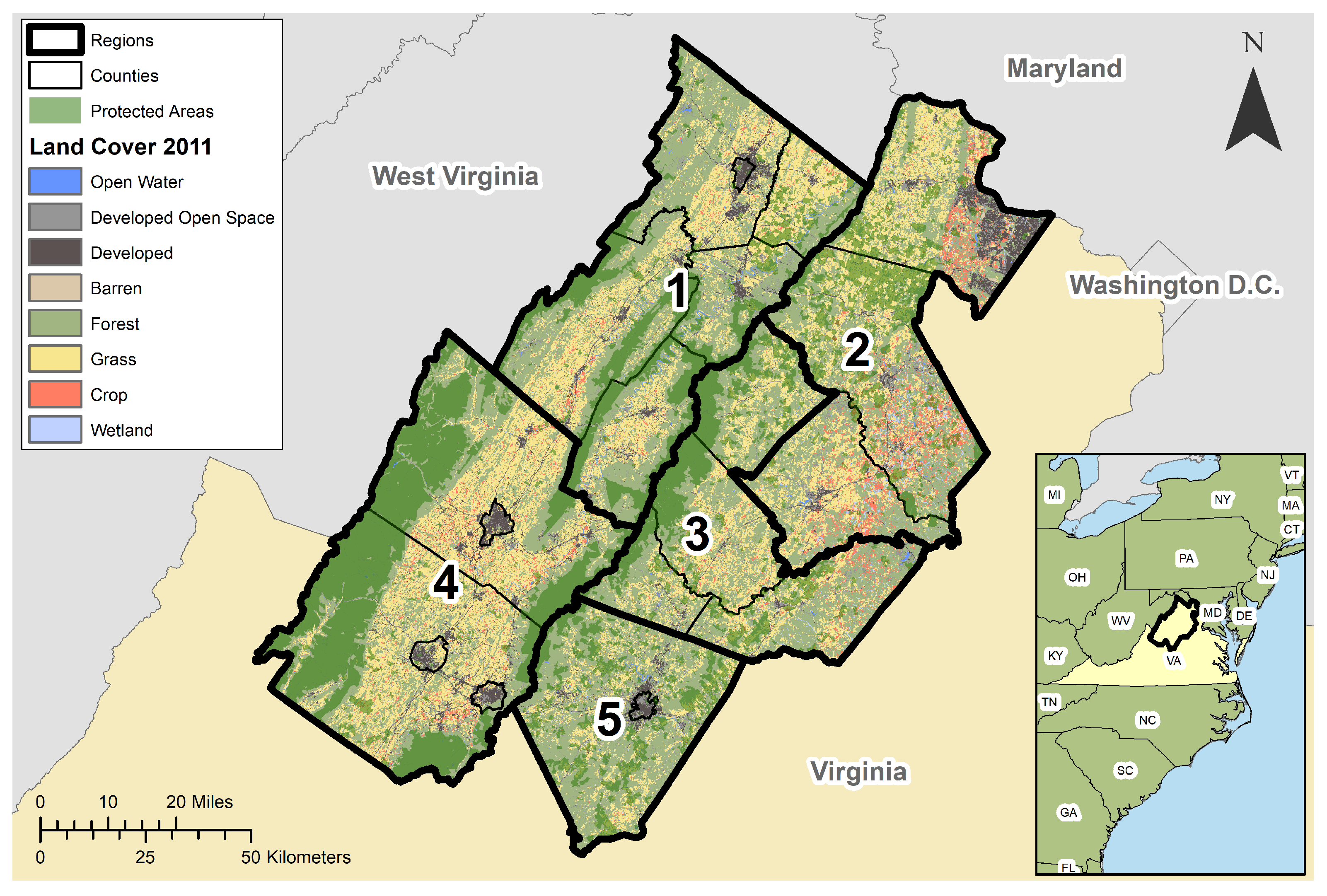
2.1. Study Area

The 17,899 km2 study area is composed of 15 counties in Virginia, USA (Figure 1). In 2011, the benchmark year for the land use change model, forests constituted the majority of land cover in the study area (~55%), followed by pastures, grassland, and other herbaceous cover (~33%) development (~7%) and croplands (~5%) ([14] Lacher et al., 2019, [15] Lacher et al., 2023). Over 25% of the study area is under some form of protected area including the Shenandoah National Park, the George Washington National Forest, and a significant number of conservation easements. To capture spatial variation in land use change dynamics, the study area was subdivided into five subregions designated by Virginia Districts Commissions and adjusted partner input. In brief, subregion 1 captures a relatively small but rapidly growing city in an otherwise rural landscape. Subregion 2 captures the highly urbanized edge of the Washington DC Metropolitan area but also a large number of affluent landowners with large properties, similar to those in development-adverse subregion 3, which also sees a more heterogeneous mixture of forests and grassland. Subregion 4 is the most agriculturally focused subregion with significant amounts of pasture but also a western edge dominated by national forest land, while subregion 5 sees the highest amount of land managed for timber in addition to a growing central city.

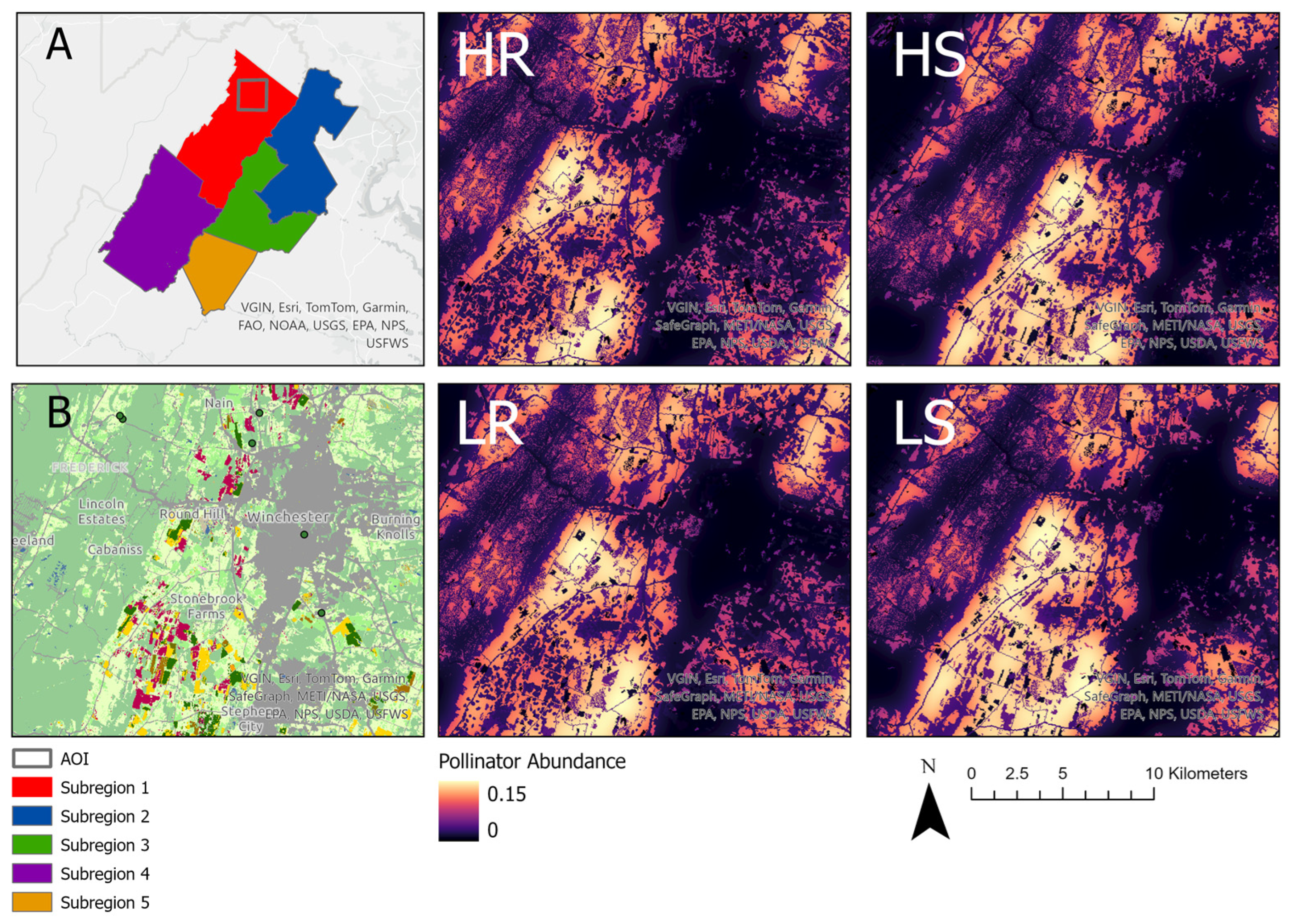
2.2. LULC Scenario Data Collection

CLI co-developed four distinct scenarios of future change in the study region ([14] Lacher et al., 2019, [15] Lacher et al., 2023). The scenario planning process engaged a broad collection of stakeholders at multiple stages of model development ([14] Lacher et al., 2019, [15] Lacher et al., 2023). Stakeholders included representatives from county planning offices, state and federal government agencies, and local to regional non-profit organizations with self-declared expertise in topics including land use planning/policy, agriculture development, and natural resource use and conservation. While [15] Lacher et al., (2023) fully described the scenario development process, we note that one workshop covering the Ridge and Valley Ecoregion (subregions 1 and 4) and a second covering the Piedmont ecoregion (subregions 2, 3, and 5) were integral to this effort. In each of the workshops, 15 to 17 stakeholders were asked to identify two key drivers of change in the subregion, consider a range of intensities for those drivers, and then estimate the impact on the landscape at the extremes of that range. The four resulting LULC scenarios were high human population growth and strategic planning (HS), high population growth and reactive planning (HR), low population growth and reactive planning (LR), and low population growth and strategic planning (LS). The CLI team then translated the stakeholder estimates of change into quantitative parameter modifications for use in a stochastic land use change model.
First, CLI modeled a business-as-usual (BAU) scenario that reflected current population and policy trends. Baseline land use change dynamics were estimated using observed changes in the National Land Cover Database (NLCD) between 2001 and 2011 and their relationship with a number of spatial covariates including slope, distance to existing development, and socio-economic factors like median income. To counter the impact of edge effects, the analysis included a 25 km buffer area. Future land use change was then projected to the year 2061 using the Program Dinamica EGO, with change occurring at the same rate as that observed and land use transition locations based on the observed variable relationships. We chose a 50-year projection window as time, which is not so far into the future to be unrealistic for stakeholders to imagine but not so short-term that the model would have enough time to diverge. To capture distinctions in growth patterns within the study area, rates of change and variable relationships were calculated and applied by subregion. In this way, each subregion effectively operated as its own independent model except for the calculation of the distance-to-development covariate, which was dynamically created at each of the model’s 10-year time steps based on the combined projections of all subregions. During this phase, stakeholders had additional input via direct communication, identifying local zoning and karst geology as important components to include as spatial covariates to ensure legitimacy with regional decision makers.
The four stakeholder-derived scenarios were then modeled using alterations to the parameters of the BAU model. A map of proximity to urban centers was used to manipulate the location of transitions to development to simulate a more centralized growth strategy for strategic planning and, inversely, a more sprawling growth strategy for reactive planning. This alteration was made for all subregions equally. High population growth was stimulated by first associating the rate of transitions to development with observed population growth and then calculating new future transition rates based on altered population growth rates. As population data were available by county, the impact of this change varied by subregion. For further details, please refer to Lacher et al., [15] (2023). For this analysis, we used all five CLI scenario landscapes as well as the observed 2011 NLCD landscape, each stored as 30 m rasters. The CLI model reduced the NLCD classes to 8 for clarity during modeling [15], and we continue with that classification here.

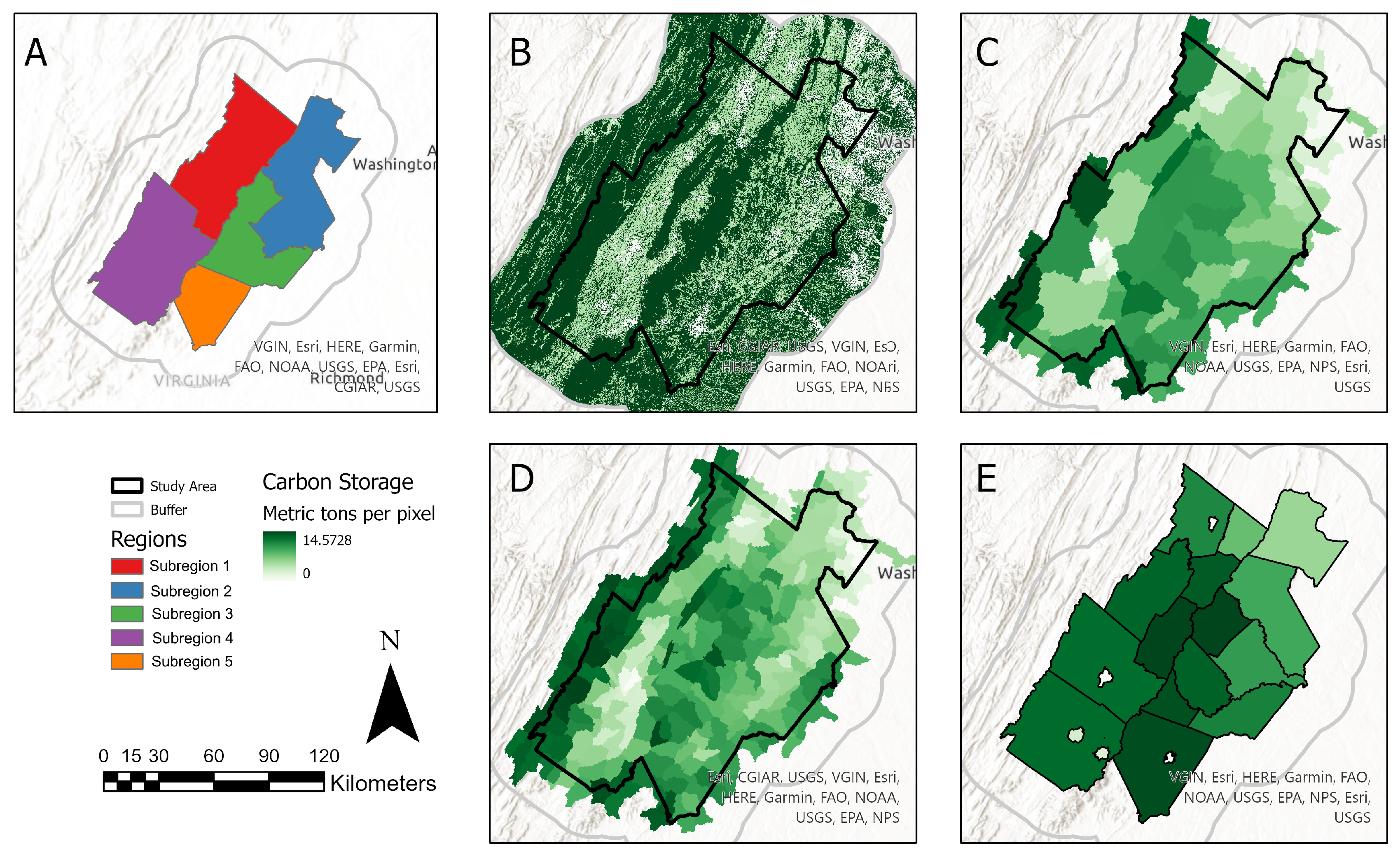
2.3. Biodiversity and Ecosystem Service Modeling

We used InVEST 3.9.0 (Integrated Valuation of Ecosystem Services and Tradeoffs), a spatially explicit modeling software that uses LULC data from within the study area and a 5 km buffer, and ecological production functions to create spatially explicit maps of ecosystem services (The Natural Capital Project, 2016). For each of the CLI landscapes, we ran 18 InVEST models: habitat quality in grassland, forest, urban, and agricultural ecosystems; spring abundance, summer abundance, and supply of three families of bee pollinators (Apis, Bombus, and Halictus); stored carbon; sediment retention; and the delivery of three disservices (nitrogen, phosphorus, and sediment). Habitat quality models reflect the known habitat value of species in an LULC type; for example, forest would be modeled as high quality for forest obligates while grassland would be low quality for these species and vice versa. For agricultural and urban models, we considered the value of these managed lands for species known to use each land use type (as compared to species that might be a forest obligate). Pollinator abundance is a measure of the per-pixel abundance in a given season for that species. Supply is a per-pixel index of pollinator species that could be present, multiplied by both habitat suitability and floral resources. We selected this particular suite of InVEST models based on feedback from CLI stakeholders as the ecosystem services they believed to be of high interest in the study region. Ecological production function input parameters for all models except pollination were drawn from [2] Brown and Quinn (2018, Table 1 and its associated supplemental file). Pollination model inputs were drawn from [1] Zhao et al., (2019, associated supplemental file). The outputs of these models were at a pixel resolution of 30 m by 30 m at the full extent of the study region, which was the smallest grain size shared with partners.

2.4. Biodiversity and Ecosystem Service Analysis

In building on the 30 × 30 m data, we also summarized data by different units of analysis. Specifically, for each scenario and the 2011 baseline, we used the exact-extract package ([17] Baston 2022) in R to calculate the mean value for each ecosystem service for multiple scales including county and watershed. For our specific quantitative case study, we used the USGS-defined HUC 12 watersheds ([18] Moore et al., 2019) in the study area. We then calculated the difference between the 2011 baseline and each of the five scenarios for each watershed. We assigned each watershed to one of the five subregions based on the location of the watershed’s centroid. We used the lme4 package ([19] Bates 2021) for linear mixed-model analysis with watershed as a random effect and scenario and subregion as fixed effects. To explain the change in each measure of biodiversity or ecosystem service, we compared four competing models: (1) scenario only, (2) subregion only, (3) subregion and scenario, and (4) the interaction between scenario and subregion. These four models allowed us to compare if modeled changes were more reflective of the scenario, the local context of a subregion, or a combination of both. We used AICc model selection to identify the best model from this set. From the top model, we based statistical inference on the 95% confidence interval not overlapping zero.

3. Results

3.1. Variation by Scale of Analysis

When sharing the data with implementing partners, we iterated the most suitable unit of analysis. In this process, we presented the raw data at 30 m by 30 m pixels (Figure 2B) and summarized each ecosystem service by different management scales in the study area defined by political and ecological boundaries including watershed, land–river segment, and county (see [16] Lacher et al., 2019) (Figure 2C–E). The different scales provided value to different partners. For example, when working to identify parcels most suited for conservation efforts that could provide carbon credits at a parcel scale, we reviewed data at the finest grain of 30 × 30 m, suggesting specific patches across the study area that would be most valuable to prioritize for protection such as large forest patches (Figure 1B). In contrast, the county-scale data (Figure 2E) provide data at a broader scale that could be used to prioritize state funds for conservation that would be delivered to county governments. We created and made available upon request similar maps for each ecosystem service.

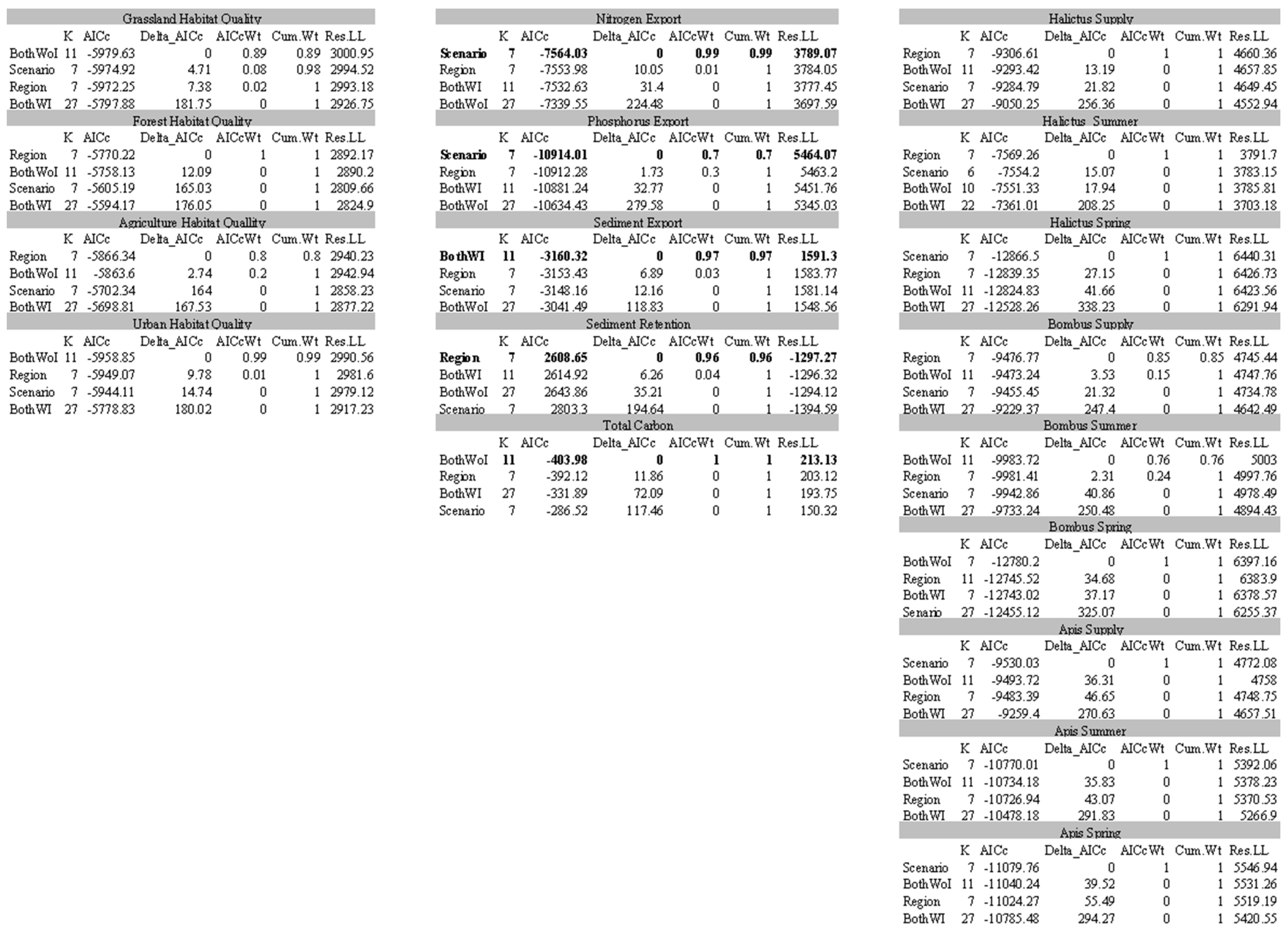
3.2. Model Selection Results

We found that the scenario-only model was the top model in seven measures of ecosystem services: the abundance of Apis in spring and summer, Apis supply, abundance of Bombus and Halictus in spring, and nitrogen and phosphorus exports (Appendix A). The subregion-only model was the top model in six other measures: Bombus supply, Halictus summer abundance and supply, habitat quality associated with sustainable agriculture and forests, and sediment retention. The scenario-and-subregion model without interaction was the top model for five measures: Bombus in the summer, habitat quality in urban areas and grassland, total carbon in the landscape, and sediment export. There were no cases where the subregion by scenario with the interaction model provided improved support.
For the most part, the general trend for the models, using intercept values as a baseline, follows what one would expect from a group of scenarios that all project overall loss of forest and growth in development between 2011 and 2061 (Table 1). Services like carbon sequestration, forest habitat quality, and multiple pollinator abundance metrics have negative trends while disservices like nitrogen and phosphorus export have positive trends. A negative trend for agriculture habitat quality is less expected given multiple scenarios projecting growth in pasture, but this is likely countered by the projected loss of cultivated crops.
We see distinctions between scenarios, however, especially the two low-population scenarios, which show significantly less negative trends in carbon sequestration and pollinator abundance. We see significantly less positive trends in nitrogen and phosphorus export compared to the BAU scenario. We also see significantly positive trends for the low-population scenarios for urban and grassland habitat quality, sediment export, and Bombus summer abundance compared to a non-significant positive intercept. The high-population strategic scenario also shows significantly less negative trends in pollinator abundance but does not show any significant differences with BAU for the other service models. Surprisingly the high-population reactive scenario, the scenario with the highest projected amount of overall change, shows no significant differences compared to BAU for any of the models.
We also see distinctions between subregions, especially with subregion 4, which shows significant distinctions for 11 of the 18 models. For forest and agricultural habitat quality, both subregions 3 and 4 show a positive trend with a magnitude higher than that of the negative trend for the reference, subregion 1. This results in an overall positive trend rather than just a less negative one. Subregion 3 shows the same for carbon sequestration while subregion 4 only shows a less negative trend. Both subregions again flip the reference trend but from positive to negative for sediment retention. Substantially negative significant differences for subregion 4 are also seen in four measures of pollinator abundance, urban and grass habitat quality, and sediment export compared to a non-significant intercept. Subregion 2 shows a significant distinction for only one model (Bombus summer abundance), and subregion 5 shows no significant distinctions for any model.

4. Discussion

By leveraging co-designed scenarios for a broad suite of biodiversity and ecosystem service models paired with subsequent interpretation of results, our transdisciplinary process was able to produce data that can be used to support land use planning around multiple conservation and management goals related to habitat, climate change, water quality, and food production.
We found that, for our full study area, the LULC differences projected by the CLI scenarios resulted in varied outcomes for biodiversity and ecosystem services. In particular, the low population growth scenarios had higher values of most measures of biodiversity and ecosystem services and reduced rates of two disservices (nitrogen and phosphorus export), suggesting population growth rates are an important driver in the region. Pollinator models, however, were also responsive to strategic planning under a high-population growth rate supporting the utility of the centralized growth strategies included in this scenario. This finding is of particular importance as in post-analysis dialogue with implementing partners, pollination services were articulated as a particular priority, which is a similar articulated value to other work implementing partners in the ecoregion ([20] Quinn et al., 2015). More broadly, these results are helpful for other policy makers in projecting the impact of regional population growth. While the results may differ in other implementations, the data suggest that regardless of reactive or strategic planning, change in population is important to understand.
However, we also found a nearly equal number of models were significantly influenced by the subregion, either where both subregion and scenario were the best model (e.g., Bombas summer) or with scenarios not showing a significant influence at all, suggesting subregion was the most important factor. This result is important as it suggests that existing regional distinctions and thus drivers of LULC change may have a stronger influence on ecosystem services than those proposed by stakeholders for the scenarios. For example, subregion 4 has a large contiguous block of forest while region 2 has greater extent croplands and urban areas. Likewise, as described in the methods, the land use and land cover change in each region was unique and reflective of local communities. This variation can guide decision makers to more closely examine the current and historic practices of the counties of the distinct subregion as examples to avoid or emulate. For example, in our study, subregion 4 showed a significant influence over the largest number of modeled ecosystem services but also presented an example of this approach being capable of identifying key tradeoffs. In this subregion, our models also project that grassland and urban habitat quality will steeply decline at the same time that habitat quality for forests and agriculture increases. This is the type of challenging tradeoff that decision makers need to be aware of to make effective conservation actions for the future. These processes provided a mechanism for local implementing partners to discuss if the projected changes are in alignment with the conservation goals for the region as a whole.
As noted in the introduction, similar ecosystem service modeling efforts have been more narrowly focused regarding their spatial extent (e.g., [8] Gibson and Quinn 2017), thus limiting comparisons across larger environmental or political boundaries. Instead, by summarizing the biodiversity and ecosystem service data at different spatial extents (pixels, parcels, watersheds, counties, and subregions, as seen in Figure 2), we are able to present the data to implementing partners in a way that is more applicable to the specific spatial decisions a given group makes. For example, organizations focused on conservation land acquisition, like workshop participants of the Piedmont Environmental Council or external groups like The Nature Conservancy, might value the patterns within a subregion composed of multiple counties. In contrast, a regional conservation planner drafting a water quality plan may find catchments of the units of the greatest value, as we found with the Rappahannock-Rapidan Regional Commission in meetings following model development. Lastly, NGOs that focus on a specific river branch or swath of land (e.g., workshop participants Friends of the North Fork of the Shenandoah and the Blue Ridge Conservation Alliance, respectively) or individual landowners managing their parcel would likely benefit most from maps displayed at the pixel scale.
Given how different end-users engage with the landscape, the dynamic options above potentially allow for cooperation between researchers and end-users more directly aligned with the management needs of differing organizations. Likewise, having co-developed scenarios reflective of both qualitative and quantitative inputs allows conservation planners and decision makers to consider the outcomes of different actions taken or values prioritized in a more meaningful way. In addition, biodiversity and ecosystem service modeling efforts, co-developed with implementing partners, allow for more suitable analyses to understand and make use of the data from chosen methods ([21] Hallett et al., 2017). Similarly, they can start to provide a “corridor of clarity”, even if imperfect, for the necessary policy action ([3] Polasky et al., 2020). From a modeling perspective, future work across spatial scales can continue to improve the direct-use value of biodiversity and ecosystem service models by leveraging the growing richness of high-resolution social and environmental spatial data layers ([22] Ordway et al., 2021) that can then be summarized at broader scales.
We did find that some changes, though not obvious in the linear mixed-modeling (LMM) results, could be clearly observed in specific areas of interest to partners. For example, for the pollination services, we found evidence of urbanization reducing pollination, particularly in agricultural subregions around cities in subregion 1 (Figure 3). Our ability to share pixel-level data at a very local scale allowed the implementing partners to see how, across the scenarios, a loss of pollination services was associated with the urbanization of an agricultural landscape. However, this pattern was not clear at the scale of the study area or subregion.
A few unresolved challenges emerged in this case study. First, across the study area, the magnitude of change in LULC in the scenarios created a challenge in detecting differences across the study area as a whole. Because the scenarios were designed to be plausible as opposed to scenarios that are more extreme or low probability ([23] sensu Groves and Game 2016), the magnitude of change and subsequent change in the different indicators was subtle. However, the realism of the scenarios has the potential to be a more credible product for users actively engaged in land use decisions. This is an interesting challenge to consider across scenario scales (e.g., between the scenarios here and the SSPs from IPCC [24]).
The second challenge was presenting and sharing the scope of the data across scenarios and models. The volume of maps produced across 5 scenarios and 18 ecosystem services presents a challenge in sharing all the data implement partners. One option in the literature is the bundling of services ([25] Cooley and Olander 2012, [26] Klain et al., 2014, [27] Saidi and Spray 2018). We avoided bundling the services in the maps or analyses. We made this choice after reflecting on the value of the data for users. We found that it would limit the ability of implementing partners to make specific choices about an ecosystem service of interest. Similarly, bundling a single value smooths out the variation in response to different drivers and reduces the information to the user, diluting their ability to make choices. That being said, the data are available for future synthesis or application by project partners.
Finally, the CLI used two years to calibrate the study area’s land use change trends, which may miss non-linear relationships or anomalous change activity. This, however, is standard practice for land use change models largely due to multiple reliable land use time steps not being available until relatively recently. We support future modeling efforts like this to explore these data as a way to improve model projection accuracy.

5. Conclusions

Biodiversity and ecosystem service models, and how subsequent results are shared and interpreted, need to better reflect the values of those who might use the data. We demonstrate that the co-development of scenarios and collaborative selection of measures of biodiversity and ecosystem services can produce distinct outputs relevant to the needs of the participants involved. We found that analysis of the InVEST models, built on high-resolution data, allowed our research team to share data at different spatial scales reflective of the need for unique implementing partners and policy makers. Lastly, our statistical analysis identified variations in the drivers of projected biodiversity ecosystem service change between scenarios and the ecosystem and governance structures that vary at subregional scales. These processes, including scenario development, ecosystem service modeling, and data synthesis, suggest that modeling efforts that are part of conservation planning can be co-developed to support the needs of a diverse range of partners while advancing the field of conservation science.

Author Contributions

Conceptualization, J.E.Q., C.F., I.L.L. and T.S.A.; methodology, J.E.Q. and C.F.; formal analysis, J.E.Q., C.F., E.H. and C.V.; resources, I.L.L. and C.F.; data curation, J.E.Q., C.F., E.H. and C.V.; writing—original draft preparation, J.E.Q., C.F., C.V. and E.H.; writing—review and editing, J.E.Q., C.F., I.L.L. and T.S.A.; visualization, E.H. and J.E.Q. All authors have read and agreed to the published version of the manuscript.

Funding

This research received no external funding.

Data Availability Statement

Input data and model results are available from the corresponding author (JQ) upon request.

Acknowledgments

We thank the reviewers for their helpful suggestions.

Conflicts of Interest

The authors declare no conflicts of interest.

Appendix A

Figure A1. AIC model selection summary for each of the 18 different InVEST models.
Land 13 01340 g0a1

References

  1. Zhao, C.; Sander, H.A.; Hendrix, S.D. Wild bees and urban agriculture: Assessing pollinator supply and demand across urban landscapes. Urban Ecosyst. 2019, 22, 455–470. [Google Scholar] [CrossRef]
  2. Brown, M.G.; Quinn, J.E. Zoning does not improve the availability of ecosystem services in urban watersheds. A case study from Upstate South Carolina, USA. Ecosyst. Serv. 2018, 34, 254–265. [Google Scholar] [CrossRef]
  3. Polasky, S.; Crépin, A.S.; Biggs, R.; Carpenter, S.R.; Folke, C.; Peterson, G.; Scheffer, M.; Barrett, S.; Daily, G.; Ehrlich, P.; et al. Corridors of clarity: Four principles to overcome uncertainty paralysis in the anthropocene. BioScience 2020, 70, 1139–1144. [Google Scholar] [CrossRef] [PubMed]
  4. Rounsevell, M.D.; Arneth, A.; Brown, C.; Cheung, W.W.; Gimenez, O.; Holman, I.; Leadley, P.; Luján, C.; Mahevas, S.; Maréchaux, I.; et al. Identifying uncertainties in scenarios and models of socio-ecological systems in support of decision-making. One Earth 2021, 4, 967–985. [Google Scholar] [CrossRef]
  5. Nelson, E.; Mendoza, G.; Regetz, J.; Polasky, S.; Tallis, H.; Cameron, D.; Chan, K.M.; Daily, G.C.; Goldstein, J.; Kareiva, P.M.; et al. Modeling multiple ecosystem services, biodiversity conservation, commodity production, and tradeoffs at landscape scales. Front. Ecol. Environ. 2009, 7, 4–11. [Google Scholar] [CrossRef]
  6. Wing, I.S.; Monier, E.; Stern, A.; Mundra, A. US major crops’ uncertain climate change risks and greenhouse gas mitigation benefits. Environ. Res. Lett. 2015, 10, 115002. [Google Scholar] [CrossRef]
  7. Terando, A.J.; Costanza, J.; Belyea, C.; Dunn, R.R.; McKerrow, A.; Collazo, J.A. The southern megalopolis: Using the past to predict the future of urban sprawl in the Southeast US. PLoS ONE 2014, 9, e102261. [Google Scholar] [CrossRef]
  8. Gibson, D.M.; Quinn, J.E. Application of anthromes to frame scenario planning for landscape-scale conservation decision making. Land 2017, 6, 33. [Google Scholar] [CrossRef]
  9. Quinn, J.E.; Wood, J. Application of a coupled human-natural system framework to identify challenges and opportunities for conservation in private lands. Ecol. Soc. 2017, 22, 39. [Google Scholar] [CrossRef]
  10. Di Marco, M.; Watson, J.E.; Possingham, H.P.; Venter, O. Limitations and trade-offs in the use of species distribution maps for protected area planning. J. Appl. Ecol. 2017, 54, 402–411. [Google Scholar] [CrossRef]
  11. Dutra Silva, L.; Brito de Azevedo, E.; Vieira Reis, F.; Bento Elias, R.; Silva, L. Limitations of species distribution models based on available climate change data: A case study in the Azorean forest. Forests 2019, 10, 575. [Google Scholar] [CrossRef]
  12. Ureta, J.C.; Clay, L.; Motallebi, M.; Ureta, J. Quantifying the landscape’s ecological benefits—An analysis of the effect of land cover change on ecosystem services. Land 2020, 10, 21. [Google Scholar] [CrossRef]
  13. Sharp, R.; Tallis, H.T.; Ricketts, T.; Guerry, A.D.; Wood, S.A.; Chaplin-Kramer, R.; Nelson, E.; Ennaanay, D.; Wolny, S.; Olwero, N.; et al. InVEST User’s Guide; The Natural Capital Project: Stanford, CA, USA, 2014. [Google Scholar]
  14. Lacher, I.; Akre, T.; McShea, W.J.; McBride, M.; Thompson, J.R.; Fergus, C. Engaging regional stakeholders in scenario planning for the long-term preservation of ecosystem services in Northwestern Virginia. Case Stud. Environ. 2019, 3, 1–13. [Google Scholar] [CrossRef]
  15. Lacher, I.; Fergus, C.; McShea, W.J.; Plisinski, J.; Morreale, L.; Akre, T.S. Modeling alternative future scenarios for direct application in land use and conservation planning. Conserv. Sci. Pract. 2023, 5, e12940. [Google Scholar] [CrossRef]
  16. Tengö, M.; Brondizio, E.S.; Elmqvist, T.; Malmer, P.; Spierenburg, M. Connecting diverse knowledge systems for enhanced ecosystem governance: The multiple evidence base approach. Ambio 2014, 43, 579–591. [Google Scholar] [CrossRef] [PubMed]
  17. Baston, D. exactextractr: Fast Extraction from Raster Datasets Using Polygons. R Package Version 0.8.2. 2022. Available online: https://CRAN.R-project.org/package=exactextractr (accessed on 9 August 2024).
  18. Moore, R.B.; McKay, L.D.; Rea, A.H.; Bondelid, T.R.; Price, C.V.; Dewald, T.G.; Johnston, C.M. User’s Guide for the National Hydrography Dataset Plus (NHDPlus) High Resolution; Open-File Report 2019-1096; U.S. Geological Survey: Reston, VA, USA, 2019; 66p. [Google Scholar] [CrossRef]
  19. Bates, D.; Maechler, M.; Bolker, B.; Walker, S.; Christensen, R.H.B.; Singmann, H.; Dai, B.; Grothendieck, G.; Green, P.; Bolker, M.B. Package ‘lme4’. Convergence 2015, 12, 2. [Google Scholar]
  20. Quinn, C.E.; Quinn, J.E.; Halfacre, A.C. Digging deeper: A case study of farmer conceptualization of ecosystem services in the American South. Environ. Manag. 2015, 56, 802–813. [Google Scholar]
  21. Hallett, L.M.; Morelli, T.L.; Gerber, L.R.; Moritz, M.A.; Schwartz, M.W.; Stephenson, N.L.; Tank, J.L.; Williamson, M.A.; Woodhouse, C.A. Navigating translational ecology: Creating opportunities for scientist participation. Front. Ecol. Environ. 2017, 15, 578–586. [Google Scholar]
  22. Ordway, E.M.; Elmore, A.J.; Kolstoe, S.; Quinn, J.E.; Swanwick, R.; Cattau, M.; Taillie, D.; Guinn, S.M.; Chadwick, K.D.; Atkins, J.W.; et al. Leveraging the NEON Airborne Observation Platform for socio-environmental systems research. Ecosphere 2021, 12, e03640. [Google Scholar] [CrossRef]
  23. Groves, C.R.; Game, E.T. Conservation Planning: Informed Decisions for a Healthier Planet; Roberts and Company Publishers: Greenwood Village, CO, USA, 2016. [Google Scholar]
  24. Samir, K.C.; Wolfgang, L. The human core of the shared socioeconomic pathways: Population scenarios by age, sex and level of education for all countries to 2100. Glob. Environ. Chang. 2017, 42, 181–192. [Google Scholar]
  25. Cooley, D.; Olander, L. Stacking ecosystem services payments: Risks and solutions. Envtl. L. Rep. News Anal. 2012, 42, 10150. [Google Scholar]
  26. Klain, S.C.; Satterfield, T.A.; Chan, K.M. What matters and why? Ecosystem services and their bundled qualities. Ecol. Econ. 2014, 107, 310–320. [Google Scholar]
  27. Saidi, N.; Spray, C. Ecosystem services bundles: Challenges and opportunities for implementation and further research. Environ. Res. Lett. 2018, 13, 113001. [Google Scholar]
Figure 1. Study region and five subregions within Virginia, USA and land use and land cover in 2011.
Land 13 01340 g001
Figure 2. (A) Map of study area and 5 km buffer. The five subregions are reflective of social and environmental factors. Amount of stored carbon in the study region summarized by (B) 30 m pixel, (C) land–river segment, (D) watershed, and (E) county.
Land 13 01340 g002
Figure 3. Change in summer abundance of Halictidae across the four scenarios (HR, HS, LR, and LS). (A) Study region with AOI. (B) Distribution of crops within the AOI (red = apples, pink = alfalfa, other crops are not bee pollinated). Data drawn from Cropscape.Pollinator abundance is a measure of the per-pixel abundance of a given species.
Land 13 01340 g003
Table 1. LMM estimates and standard error (SE) for habitat quality, carbon, nitrogen, and phosphorus exports, sediment, and pollination. Estimates in bold have 95% CI that do not overlap zero. Blanks were model parameters not included in the top AICc model.
Apis SupplyApis SpringApis SummerBombas SupplyBombas SpringBombas SummerHalitctus SupplyHalitctus SpringHalitctus Summer
EstSEEstSEEstSEEstSEEstSEEstSEEstSEEstSEEstSE
Intercept−0.00130.0002−0.00070.0001−0.00060.00010.00030.0005−0.000190.000040.00020.00040.00030.0005−0.00020.000040.00010.0005
ChangeHS0.00030.00010.00010.00010.00010.0001 0.000050.000020.00020.0001 0.00000.00002
ChangeHR−0.00010.0001−0.00010.00010.00000.0001 0.000000.000020.00010.0001 0.00000.00002
ChangeLR0.00060.00010.00030.00010.00040.0001 0.000140.000020.00060.0001 0.00010.00002
ChangeLS0.00080.00010.00040.00010.00040.0001 0.000140.000020.00050.0001 0.00010.00002
Region2 0.00130.0007 0.00120.00060.00120.0008 0.00110.0007
Region3 −0.00010.0006 −0.00050.0004−0.00020.0006 0.00010.0006
Region4 −0.00320.0007 −0.00290.0005−0.00330.0007 −0.00270.0006
Region5 0.00050.0010 0.00030.00080.00050.0010 0.00040.0009
Total CarbonNitrogen ExportPhosphorous ExportSediment ExportSediment Retention
EstSEEstSEEstSEEstSEEstSE
Intercept−0.42650.04730.00320.00050.00080.00010.02510.01732.07350.2744
ChangeHS0.01890.01360.00080.00030.00000.00010.00320.0028
ChangeHR−0.01870.0136−0.00040.00030.00000.00010.00130.0028
ChangeLR0.03690.0136−0.00150.0003−0.00030.00010.01610.0028
ChangeLS0.06930.0136−0.00050.0003−0.00030.00010.01400.0028
Region2−0.07180.0670 −0.03250.02400.73080.3906
Region30.52500.0597 −0.03650.0155−2.17500.3131
Region40.40360.0637 −0.11770.0233−3.29220.3747
Region50.09120.0898 −0.03290.0350−0.59580.5420
Urban Hab. Qual.Agriculture H. Qual.Forest H. Qual.Grassland H. Qual.
EstSEEstSEEstSEEstSE
Intercept0.00470.0031−0.02770.0030−0.02840.00320.00320.0030
ChangeHS0.00130.0007 0.00130.0007
ChangeHR0.00040.0007 0.00030.0007
ChangeLR0.00450.0007 0.00430.0007
ChangeLS0.00400.0007 0.00400.0007
Region2−0.00190.0044−0.00330.0044−0.00460.0046−0.00240.0042
Region3−0.00830.00340.03730.00360.03830.0038−0.00630.0034
Region4−0.02400.00420.03340.00420.03330.0044−0.02190.0041
Region5−0.00050.00610.00710.00600.00690.00630.00020.0059
Disclaimer/Publisher’s Note: The statements, opinions and data contained in all publications are solely those of the individual author(s) and contributor(s) and not of MDPI and/or the editor(s). MDPI and/or the editor(s) disclaim responsibility for any injury to people or property resulting from any ideas, methods, instructions or products referred to in the content.

