Article

Deciphering Motorists’ Perceptions of Scenic Road Visual Landscapes: Integrating Binocular Simulation and Image Segmentation

by
Zhaocheng Bai
1,
Rui Ji
2 and
Jun Qi
1,3,*
1
College of Landscape Architecture and Horticulture, Southwest Forestry University, Kunming 650224, China
2
College of Architecture and Urban Planning, Tongji University, Shanghai 200092, China
3
Southwest Research Center for Landscape Architecture Engineering, State Forestry and Grassland Administration, Kunming 650224, China
*
Author to whom correspondence should be addressed.
Land 2024, 13(9), 1381; https://doi.org/10.3390/land13091381
Submission received: 7 August 2024 / Revised: 26 August 2024 / Accepted: 27 August 2024 / Published: 28 August 2024

Abstract

:
Traditional scenic road visual landscape assessment methods struggle to quantify drivers’ subjective visual perceptions. This study aims to develop a new method to decipher Scenic Road Visual Landscape Evaluation (SRVLE) of motorists’ visual field, reconciling the longstanding subjectivity–objectivity dichotomy in landscape quality research. By adopting binocular visual simulation and image segmentation, this paper conceptualizes a novel “non-scale semantic differential approach” to quantify landscape qualities across the dimensions of naturalness–artificiality (NA), diversity–coherence (DC), and openness–deepness (OD), constructing a three-dimensional visual landscape quality evaluation system. Taking the Nujiang Beautiful Road in Yunnan as a case study, the results show the following: (1) The three indicators reveal the scenic road’s distinctive visual landscape characteristics, marked by high naturalness, coherence, and relative openness. (2) SRVLE is found to vary between the two driving directions and different sections. (3) The three-dimensional evaluation cube intuitively displays the comprehensive characteristics of landscape quality, providing a basis for scenic road planning. This method offers a new approach to resolving the subjective–objective divide in SRVLE and can assist road administrations in enhancing policy planning, construction, and management, thereby promoting the high-quality development of scenic roads.

1. Introduction

Scenic roads are recreational transportation routes built by leveraging natural corridors such as mountains, rivers, and heritage corridors including ancient city walls and trade routes. They are the product of the integration of transportation, tourism, and landscape [1,2] and are considered an antidote to monotonous travel [3]. Scenic roads built upon roadside landscape resources can provide countryside driving experiences and nature tourism services, allowing the “charm value” of the road to surpass its “mobility value”, with the road itself becoming a destination [2]. In developed countries, scenic roads have evolved from parkways, initially serving horse-drawn carriages and then experiencing rapid development after the invention of the internal combustion engine [4]. With the development of the transportation industry, scenic roads have extended the leisure travel activities of urban residents from city parks to suburban and national park areas [5], such as the Blue Ridge Parkway in the US in the 1930s and the German Alpine Road. However, in developing countries, transportation has developed prior to the leisure tourism industry, and the two have long remained in a state of separation. Roads often fail to showcase the beautiful landscapes along the way and may even damage the natural scenery due to construction work, hindering the development of the tourism industry [6,7]. In recent years, some developing countries have begun to attach importance to the significance of scenic road construction, seeing it as an effective economic means to achieve the integration of landscape resources and coordinated regional development, and it has even been regarded as an important national development strategy in China [8].
Roadside landscapes are the core resources of scenic roads, comprising the comprehensive whole of all land and the spatial and material elements on the land that are within the driver’s line of sight [9]. For self-driving travelers, from the perspective of the mobility experience, the landscapes and spaces change with the travelers’ movement and are the primary source of travel pleasure [10]. Therefore, improving the visual landscape quality of scenic roads is the main goal of their construction, and evaluating the visual landscape quality is the foundational work and basis for the planning, construction, and management of scenic roads [3,9,11].

1.1. Objectivity vs. Subjectivity in Scenic Road Visual Landscape Evaluation (SRVLE)

Similar to the general understanding of visual landscape evaluation, the SRVLE is also divided into expert and public paradigms based on the type of evaluator [12,13]. The expert paradigm prioritizes the objective expression of the physical characteristics of the road landscape, focusing on the scientific rigor and accuracy of visual landscape quality research [14]. The public paradigm prioritizes the subjective expression of the perceived experience of the road landscape, focusing on the humanistic nature and public benefit of visual landscape quality [15].
The expert paradigm originated in the 1960s [16], with professionals from various fields such as transportation, design, ecology, commerce, and tourism objectively evaluating the physical attributes of the landscape elements, such as form, color, line, and space, combined with available information on topography, climate, and biodiversity [14]. This often involves multiple complex aspects such as scenic value, natural value, historical value, recreational value, and cultural value [17,18]. The first set of expert evaluation systems for road landscape was the Visual Impact Assessment (VIA) established by the US Federal Highway Administration in 1986, which was later introduced into the US National Scenic Byway Program, marking the standardization of the scenic road evaluation process [16,19]. In China, the expert paradigm was introduced to the scenic road field around 2000: scholars such as Wu Bihu invited a panel of 10 experts from related fields to use the “equidistant expert group visual assessment method” to conduct on-site investigation and evaluation of the natural landscape, cultural landscape, viewshed, and visual quality of the Xiao Xing’an Mountains Scenic Road every 1 or 2 km [20]. Although the expert paradigm’s evaluators are also human beings who need to establish multi-dimensional indicators and score through field investigations and data collection [21], at this stage, the “human” is merely a “professional machine” under the evaluation standards, striving to completely eliminate subjective emotions and make objective physical descriptions [22]. With the development of geographic information technology, remote sensing imagery, land cover, and elevation data have been used for objective quantitative analysis of visual landscape quality [23]. RVLQA often focuses on spatial feature analysis [24] or visibility calculation [22] or combines viewshed analysis results with landscape characteristics such as land use and ecological patterns to provide a quantitative basis for planning and design [25]. For example, Anderson et al. conducted viewshed analysis based on the digital surface model (DSM) generated from LiDAR data to evaluate the visual landscape quality of the Blue Ridge Parkway in terms of the visibility of various landscapes during the driving process, thereby managing the roadside landscape [26]. The introduction of geographic information methods has made the expert evaluation process less subject to the interference of personal subjective perception; accordingly, they are considered a more scientific set of methods [27], and due to the standardization and universality of the methods, they have been promoted in various countries as the official procedures for scenic road assessment and construction [18,28].
The public paradigm holds that the perceived authenticity of visual landscapes is more important, and the remote sensing and other materials used in the expert evaluation have a large difference in perspective from the users; therefore, they cannot represent the public’s perception [29,30]. Clay and Smidt [3] have demonstrated that the public and experts have different focuses in road landscape evaluation and even show different preferences for the same evaluation content. Therefore, the public paradigm believes that visual landscape quality is the joint product of the specific (visible) characteristics of the landscape and the psychological (perceptual, cognitive, and emotional) processes of the human observer; without an observing subject, there is no visual landscape, and the evaluation results need to be based on the subjective aesthetic values of the people [31,32]. The paradigm of public evaluation is to express the subjective feelings of the users, using photos, images, etc., as the presentation medium and relying on surveys, scales, etc. to obtain a visual landscape quality evaluation [15,25]. For example, Kent and Elliott [17] took photographs of a scenic road in Connecticut, USA, and invited 177 residents along the route to score the selected photographs to obtain information on the landscape quality of that road segment. Matijošaitienė and Stankevičė [33] established a web-based questionnaire with multiple sets of conceptual semantic differentials, such as “interesting–boring”, “natural–artificial”, and “harmonious–chaotic”, and invited subjects to evaluate 288 road landscape photos along 12 major European traffic routes in Lithuania. The evaluation methods of the public paradigm based on questionnaires and scales have been criticized by the expert paradigm: (a) there are quite obvious subjective differences between different groups and even individuals within the same group [15,31]; (b) the scales used in most studies have a large span and ambiguous expression, and their reliability and validity are difficult to verify [32,34]. Therefore, the expert paradigm criticizes the RVLQA of the public paradigm as being difficult to quantify, unscientific, and unable to support the needs of planning and construction [22,35].
The “objectivity of evaluation” in the expert paradigm and the “subjectivity of experience” in the public paradigm have become two sides that cannot be reconciled in the process of exploring the visual landscape quality of scenic roads. Some studies have attempted to integrate the advantages of the two paradigms. For example, Martín et al. [25] have combined the observer’s perspective with the traditional landscape planning perspective, using photos to supplement the attributes that are difficult to observe from flat maps, and believe that the expert paradigm with the assistance of the public paradigm can provide more detailed references for road planning and design. However, such methods only use the two paradigms simultaneously and have not achieved the objective quantification of subjective visual perception; therefore, the results obtained from the two paradigms may contain contradictions. Some scholars working with the public paradigm, based on the “stimulus–response” principle [14], have conducted quantitative analysis of the visual preferences of scenic road visitors through eye movement data, EEG, ECG, and other physiological indicators in an attempt to objectively express subjective perceptions, and they believe that this method can scientifically and accurately serve in the planning and construction of roadside landscapes [9]. However, this method confuses aesthetic preferences and visual perception; it quantifies physiological signals to measure preferences but does not quantify the visual landscape elements themselves. As a result, it remains unclear how to relate preferences to landscape quality or control the quantity and quality of visual landscape elements in planning and design. In recent years, the rapid development of the computer vision field has provided new intelligent tools for visual landscape research, which have been widely used in urban street environments to quantitatively describe street landscape characteristics such as the green view index and the sky view factor [36,37]. However, such studies rely on street view big data and have not applied their methods to scenic roads.

1.2. Eye Range vs. Proportional Reality: Expressing the Visual Landscape

Images, as authentic records and remote representations of landscapes, are an important medium for visual landscape evaluation for both the expert and public paradigms [38]. However, how to comprehensively and scientifically express visual landscapes through photographs has not yet been resolved. Some studies suggest that a 50 mm focal length camera lens can provide an experience similar to the human eye, with a more natural perspective effect [39,40]. Therefore, some visual landscape evaluation studies have used this focal length to collect image data [3,41,42]. However, the actual field of view of this focal length is significantly narrower than that of the human eye (only 60° of view) and can only record limited visual information [43]. A comparative study found that the visual landscape evaluation based on ordinary camera photos had obvious differences from on-site perceptual evaluation and attributed this to the incomplete expression of the scene by photos [44]. Therefore, some scholars believe that panoramic images can cover the full range of human vision and are more suitable as a medium for landscape visual evaluation [21]. Panoramic images have gradually been widely adopted in the field of visual landscape research [45,46,47] and have also been used in audits of built urban street environments [48,49]. However, in reality, untreated panoramic images have large distortions, and the image content is distorted, with incorrect proportions of various elements, deviating significantly from real human visual perception [50]. Pardo and Mérida [51] shot multiple overlapping photos from the same viewpoint and then stitched them into a super-wide-angle image to eliminate the distortion of a single shot in order to evaluate the visual landscape of a roadside viewing point in Spain. There has also been research in which photos were taken in four directions (north, east, south, and west) from the same viewpoint (without stitching them together) to fully present the visual landscape of a street scene [52]. However, these methods have large data volumes and complex processing, and the latter method divides the landscape scene into different pictures, causing discontinuity in the visual experience during the evaluation process. Virtual reality (VR) scenarios can be created using panoramic images or 3D modeling, allowing evaluators to be immersed and obtain a comprehensive view. Gandy and Meitner [53] introduced VR scenarios into the evaluation process to help subjects accurately perceive and express their visual experience of a scenic road, but such methods have higher time and monetary costs, making them difficult to popularize [54]. The media for visual landscape evaluation are constantly pursuing true simulation of human visual perception, but there are few cases that can effectively simulate the human binocular visual experience. Little research has started from the physiological characteristics of human binocular vision to produce visual landscape evaluation images that are closest to the human visual field.
Based on the identified research gaps, this study aims to break through the limitations of the two existing research paradigms in the field of SRVLE. On one hand, from the perspective of visual physiology, it will collect scenic road image data based on the characteristics of the binocular field of view (FOV) to address the subjectivity of the viewing experience. On the other hand, it will utilize semantic segmentation to process the images, ensuring the objectivity of the evaluation data through pixel-level analysis of object information. This study will empirically apply the new SRVLE methodology to the Nujiang Beautiful Road in Yunnan, China. The main steps include road image acquisition, integration of the human eye’s FOV, image segmentation, and perception indicator calculation to analyze the visual landscape quality as perceived by self-driving travelers. This research will provide value for scenic road landscape evaluation and management, and it also has broad applicability in the field of environmental assessment.

2. Materials and Methods

2.1. Study Area

The Nujiang Beautiful Road is a scenic route spanning approximately 282 km within the Three Parallel Rivers Protected Areas, a UNESCO World Heritage Site, adjacent to the China–Myanmar border. The northern terminus of the road is located in Bingzhongluo Town, Yunnan Province, China (28.013333° N, 98.628471° E), while the southern end lies in the northern outskirts of Lushui City (25.904833° N, 98.833333° E). Traversing the Hengduan Mountains region, this 282-kilometer stretch is characterized by rugged terrain featuring four mountains and three rivers. This winding high-altitude road offers drivers the opportunity to appreciate the renowned Nujiang Grand Canyon, known for its scenic beauty. The canyon presents impressive landscapes including forests, rivers, glaciers, and high-altitude karst formations (Figure 1). Since 2017, the local government has invested over RMB 7 billion to improve road infrastructure, enhance tourist facilities, and upgrade the scenic beauty of the road, thereby enriching the tourist experience [55]. As this location is a designated scenic road tourist destination, its landscape resources warrant attention.

2.2. Image Acquisition and Simulation of the Human Eye’s Field of View

2.2.1. Acquisition Equipment

To address the incompleteness of using regular photographs in place of the human eye’s field of view and the one-sidedness of the landscape evaluation results, a convenient, fast, and low-cost simulation method for the human eye’s field of view is proposed. According to visual physiology research, the binocular visual range of a person generally refers to the entire spatial range observed by the human eye within the horizontal and vertical planes, with the head and eyes fixed and not rotating [56,57], and the normal adult’s monocular visual field is generally 150° horizontally (60° inward and 90° outward from the cheek) and 125° vertically (55° downward and 75° upward). The binocular visual field has about 120° of overlap in the horizontal direction, resulting in a 180° horizontal and 125° vertical visual field [58].
This study selected the Insta360 ONE X2 action camera (X2 camera) as the image acquisition device for the roadside landscapes of the Nujiang Beautiful Road. This device has been applied in urban and suburban environments and has shown good acquisition performance [59,60]. The X2 camera has an equivalent focal length of 7.2 mm and can capture 360° panoramic photos in both the horizontal and vertical directions when both the front and rear lenses are working. Although the images have significant distortion around the edges, the central area retains good perspective realism, and this perspectively accurate imaging area is larger than the human eye’s field of view. Additionally, this action camera has the following advantages: (1) it is small, portable, and easy to install and firmly mount on the vehicle; (2) it has excellent motion capture capabilities, ensuring high-quality imaging under high-speed and vibration conditions; (3) it has a mobile app control function, providing convenience for in-vehicle shooting; (4) it has a GPS function, effectively recording the shooting location; (5) it has good waterproof and dustproof performance, ensuring high reliability in complex shooting environments.

2.2.2. Bidirectional Equidistant Photo Acquisition

Previous visual landscape quality evaluation studies have used photos selected subjectively by researchers [15,25,33], which has affected the comprehensiveness and objectivity of road quality expression, and may have led to biased evaluations by participants. This study uses a bidirectional equidistant photo acquisition method to comprehensively present the road landscape environment. Regarding the selection of shooting distance, relevant visual physiology research has shown that the human eye can distinguish the color and form of objects at a distance of 1 km but cannot clearly distinguish the outlines of landscape entities beyond 1 km [61,62]. One previous SRVLE research has also set a 1–2 km observation interval to record the landscape changes along the road [20]. This study adopted a 1 km photo acquisition interval, resulting in 282 sampling points in each direction, which ensured the continuity and accuracy of the road landscape description while maintaining relatively little landscape overlap between adjacent images. Furthermore, regarding the actual driving experience, the Nujiang Beautiful Road has cliffs on one side and the Nujiang River on the other, resulting in differences in landscape experiences in the two driving directions. Therefore, bidirectional acquisition was necessary.
To better present the roadside landscapes, images were collected on weekdays (26–30 April 2021), shortly after the road was newly constructed and opened, to minimize interference from other vehicles. The Nujiang Beautiful Road has a speed limit of 40 km/h throughout its length. During image acquisition, we deliberately maintained a vehicle speed of approximately 30 km/h and ensured a stable posture to minimize vibrations. We also took care to avoid interference from other vehicles on the road. While our target image acquisition interval was 1 km, slight variations of a few dozen meters were necessary in some cases to maintain a distance from the preceding vehicle. Additionally, the camera was fixed at a height of 1.2 m above the ground, perpendicular to the vehicle’s hood, to match the typical eye level of a driver. The camera parameters were set to 360° panoramic shooting, with GPS positioning enabled and other parameters kept consistent to reduce differences in image quality.

2.2.3. Synthesis of Binocular Field of View Images

The panoramic images captured by the X2 camera need to go through four steps, namely, software export, preliminary cropping, distortion correction, and field-of-view simulation, to obtain images that closely match the driver’s binocular visual field (Figure 2). The most critical step is to utilize Python’s PIL library to apply the visual field range proposed by Ruch and Fulton [58] to crop the research images, retaining only the area within the visual field, thereby obtaining images of the Beautiful Road matching the human eye’s field of view.

2.3. Segmentation of Visual Field Images

Identifying and segmenting the landscape elements in the images is crucial for the objective measurement of scenic road visual landscape quality. This study employed semantic segmentation and pixel analysis to quantify the driver’s visual perception, utilizing the Gluon CV toolkit integrated with the DeepLabv3+ model based on Apache MXNet. Gluon CV simplifies model development and offers a range of pre-trained models, including DeepLabv3+, which is known for its accuracy and efficiency, especially in road scene segmentation [63]. When tested on the ADE20K dataset, DeepLabv3+ outperformed other models such as PSPNet and SegNet, achieving 82.1% pixel classification accuracy [63]. This approach generates labeled images, enabling precise calculation of area proportions for each landscape element, thereby supporting objective assessments of scenic road environments. The combination of Gluon CV, DeepLabv3+, and the ADE20K dataset has been used to identify street environment elements [52,64].

2.4. Constructing the SRVLE System

To address the reliability issues caused by the coarse intervals of traditional semantic differential scales, this study constructed a “non-scale semantic differential approach”. It utilizes pixel-level image calculations to obtain more precise numerical values for detecting scenic road visual landscape quality. To ensure comparability between different dimensions, each concept pair is set as an indicator ranging from 0 to 1, with 0 and 1 representing the two extremes. The terms “high value” and “low value” only reflect the degree of proximity to the maximum or minimum and do not indicate the overall quality level.
In selecting the concepts for the semantic differentials, this study refers to the visual landscape evaluation framework proposed by Ode et al. [65] in the EU project VisuLands, as well as the related content of the US Federal Highway Administration’s Visual Impact Assessment (VIA) system [66]. Considering the actual conditions of the case study site and the requirements of photo evaluation, three pairs of semantic differential indicators were finalized: “Naturalness–Artificiality (NA)”, “Diversity–Coherence (DC)”, and “Openness–Deepness (OD)”. These examine the landscape’s ecological attributes, compositional elements and spatial characteristics. The definition and calculation method for each indicator are as follows:

2.4.1. Naturalness–Artificiality (NA)

The NA attribute of the landscape refers to the degree of human modification of the natural environment. A more natural and primitive landscape character can evoke a sense of freshness and pleasure for self-drivers [67,68]. However, the quality of the landscape cannot be judged simply by the NA value; well-designed artificial elements, such as service areas and observation decks, can also enrich the driving experience by providing necessary amenities.
In the expert paradigm’s environmental audits, geographic information technology is often used to calculate the area and weight of different land cover types to assess this indicator [25,69]. This study constructed the NA perceptual characteristics of the roadside landscape (except the driving road) from the driver’s perspective by considering the type of landscape objects and their proportional coverage in the visual field. The landscape objects were divided into natural elements (e.g., trees, shrubs, mountains, and sky) and artificial elements (e.g., buildings, fences, walls, and signs). The ratio of visual coverage between natural and artificial elements reflects the degree of NA in the landscape.
N A = i = 1 n s N i
where n is the number of natural elements and s N i represents the proportion of the ith natural element in the roadside landscape. NA is the sum of the area proportions of all natural landscape elements. An NA value closer to 1 indicates a more natural landscape.

2.4.2. Diversity–Coherence (DC)

DC measures are commonly used indicators in visual landscape evaluation. In the scenic road driving context, diverse landscapes can enrich the visual experience and relieve visual fatigue and stress [70]. However, excessive elements may reduce harmony and potentially pose safety risks by distracting drivers [71,72]. Additionally, coherent landscapes have a sense of order, but lack of variety can lead to monotony [73].
Most scholars calculated DC based on information entropy theory [74,75]. However, information entropy essentially reflects the uncertainty and discreteness of elements, which is not equivalent to diversity and richness [76,77]. This study calculated DC based on the principles of compositionism [78,79] and introduced the concept of “thematicity” to improve the measurement. DC involves two aspects: (a) Element quantity. The more types of elements, the more diverse the landscape. (b) Element thematicity. Significant differences in the area proportions of elements indicate visually dominant features, resulting in a unified landscape theme. If each element contributes a similar proportion of the FOV, the resulting landscape appears more chaotic.
D C = N N s S D
where N is the number of element labels in the image, N s is a constant representing the typical 15 landscape element types in this case, and SD is the standard deviation of the proportions of different labels. A DC value closer to 1 indicates a more diverse landscape.

2.4.3. Openness–Deepness (OD)

The OD reflects the degree of spatial enclosure. Open road spaces can make self-drivers feel relaxed and safe [80,81]. Deep road spaces bring a sense of mystery and focus, causing drivers to concentrate [71]. The calculation of OD depends on the proportion of environmental background within the visual field. In urban studies, OD is calculated using sky visibility [71]. In the scenic road environment, there are no high-density buildings or congested traffic; therefore, the road can also be an environmental background.
O D = S s + S r S f
where S s and S r are the areas of sky and road in the image and S f is the total image area. An OD value closer to 1 indicates a more open landscape.

3. Results

3.1. Semantic Segmentation Results

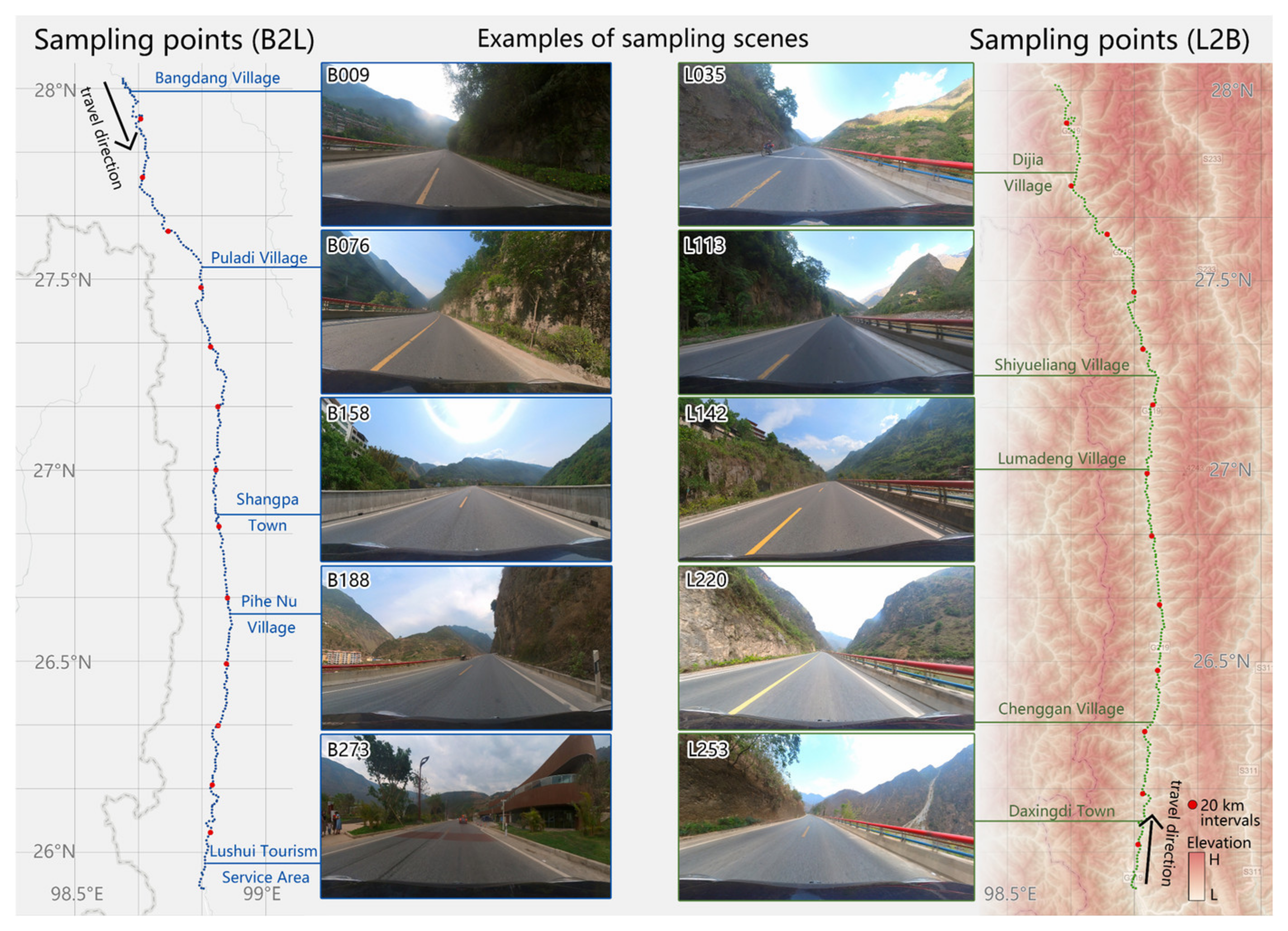
This study set up 282 sampling points in both the Lushui–Bingzhongluo (L2B) direction and the Bingzhongluo–Lushui (B2L) directions. Among the 564 road images captured at all sampling points, 560 photographs were successfully captured (Figure 3), with four missing in the L2B direction. The missing data occurred due to temporary connectivity issues between the phone and the camera. To maintain the rigor of our analysis, these four missing values were filled using interpolation (average of adjacent values). Due to the round-trip shooting, the two shooting series have opposite geographic shooting orders. The results in the L2B direction are arranged in reverse order to facilitate data comparison.
The image segmentation identified 15 landscape element labels in the case study area: tree, shrub, mountain, water, sky, driving road, other road, building, wall, fence, bridge, bare land, sign, vehicle, power pole/tower, and unidentified (Table 1). It is worth noting the following: (a) Since the vehicle is not a fixed roadside landscape and the labels identified as “undefined” are mainly due to individual errors, these two items were excluded from the index calculation process. (b) The tunnel, a special road scene (road and wall only), has extremely low NA, DC, and OD values, which will have a large impact in the calculation. Therefore, image data taken inside the tunnel were excluded in the specific analysis.
The semantic segmentation results revealed the following: (a) the Nujiang Beautiful Road has a rich variety of landscape elements, but with significant disparities in their proportional coverage within the visual field. Four landscape elements—the driving road, mountains, sky, and trees—occupy over 90% of the visual field, forming the fundamental basis of the scenic road’s visual landscape. (b) Among these elements, mountains, trees, and sky exhibit the highest standard deviations in their visual field proportions, indicating the greatest variation and dynamism in the driving experience, providing a more varied visual perception. (c) Comparing the data between the two driving directions, the proportional coverage of the same landscape elements fluctuates slightly, but the differences remain within 3%, suggesting a high degree of similarity in the overall visual landscape characteristics along the case study site.

3.2. NA Evaluation

The evaluation results show that the overall NA value of the Nujiang Beautiful Road is 0.9050 (with L2B at 0.8994 and B2L at 0.9105) (Table 2). The higher NA values along the Nujiang Beautiful Road are concentrated in the middle to late sections of the road (north of Lushui City), as the endpoints of the road are still some distance away from the Lushui city center, where the natural landscape is well preserved. However, as the road passes through several townships along the way, the occasional appearance of villages leads to fluctuations in the NA index, with the lowest NA value reaching 0.5366. Nevertheless, due to the sparse population and low building density in the region, the occurrence of these lower NA values is sporadic.
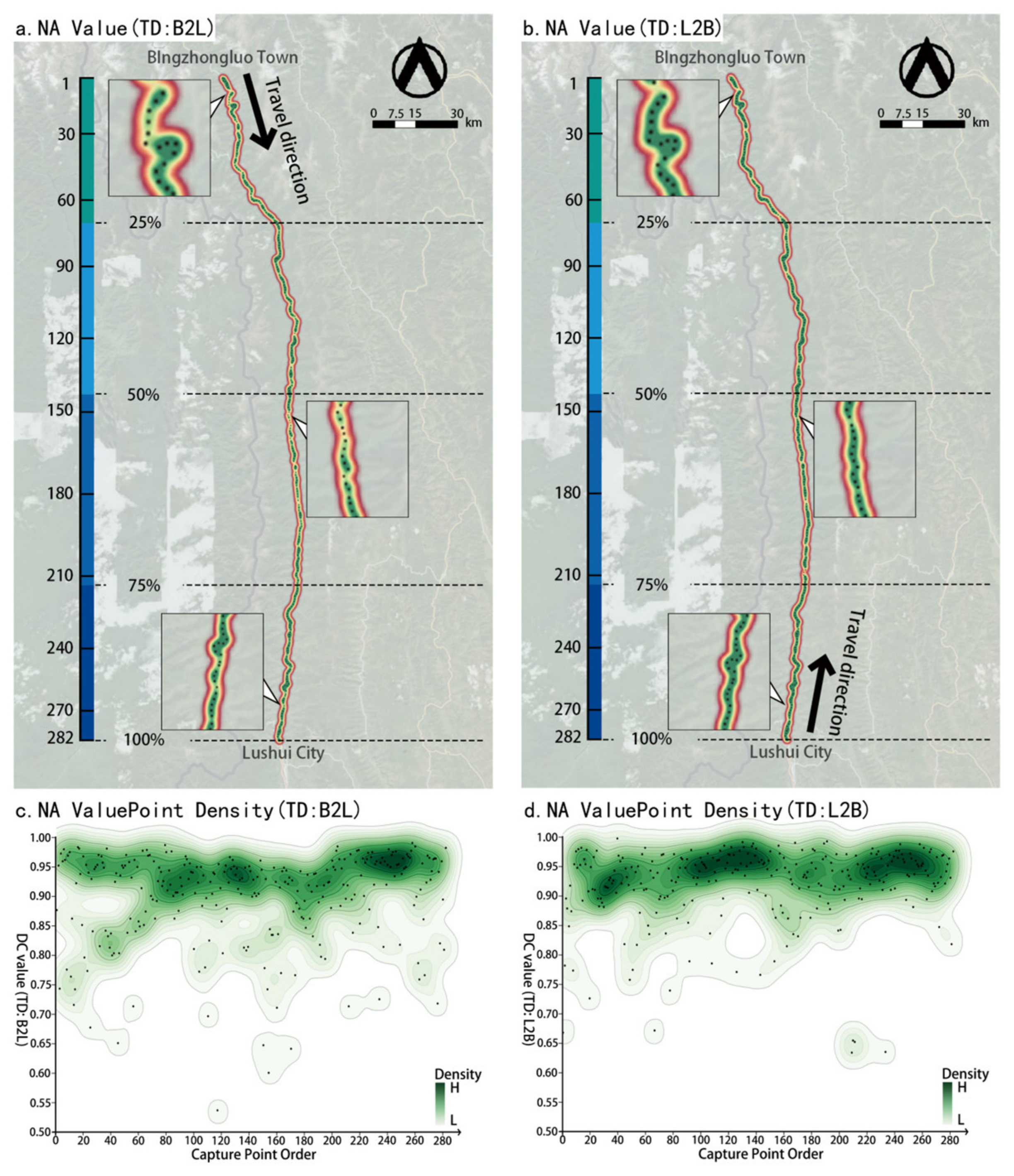
Overall, the Nujiang Beautiful Road exhibits a high degree of similarity and synchronous changes in the NA values on both sides of the road. However, analysis of the NA heatmap and point density plot (Figure 4) reveals certain differences between the two driving directions. The B2L direction shows a more continuous and concentrated distribution pattern, while the L2B direction has a more scattered distribution with greater fluctuations in NA values. To validate the differences in NA distribution characteristics, kurtosis was calculated. The kurtosis is higher for the B2L direction (8.5023) compared to the L2B direction (5.6591), indicating a more significant clustering of NA values around the mean in the B2L direction.
The B2L side exhibits a higher average NA value. However, the proportions of landscape elements reveal that the B2L direction has smaller visual shares of five natural landscape elements (trees, shrubs, mountains, water bodies, and bare land) compared to the L2B direction. This discrepancy arises because the B2L side lies on the outer edge of the road, nearer to the Nujiang River and farther from the mountains, resulting in a broader sky view and fewer artificial elements interrupting the natural landscape. In contrast, the L2B direction is closer to the mountains and features more road infrastructure (such as retaining walls). Although these elements are also visible from the opposite side, they occupy a smaller proportion of the visual field.

3.3. DC Evaluation

The L2B side has an average of 6.25 elements per image, while the B2L side has 6.79 elements (Table 3). The three dominant theme elements (mountains, trees, and sky) and the two inherent road features (driving road and guardrails) appear frequently and continuously. After excluding these five element types, the additional landscape elements that appear at each sampling point are considered the key factors contributing to visual stimulation. These key factors are mainly water bodies, shrubs, and buildings, which enrich the landscape experience. It can be observed that each image has about one additional key factor. The DC values are 0.2839 for the L2B direction and 0.3198 for the B2L direction, both less than 0.5. Overall, the landscape of the Nujiang Beautiful Road can be characterized as coherent but not lacking in interest.
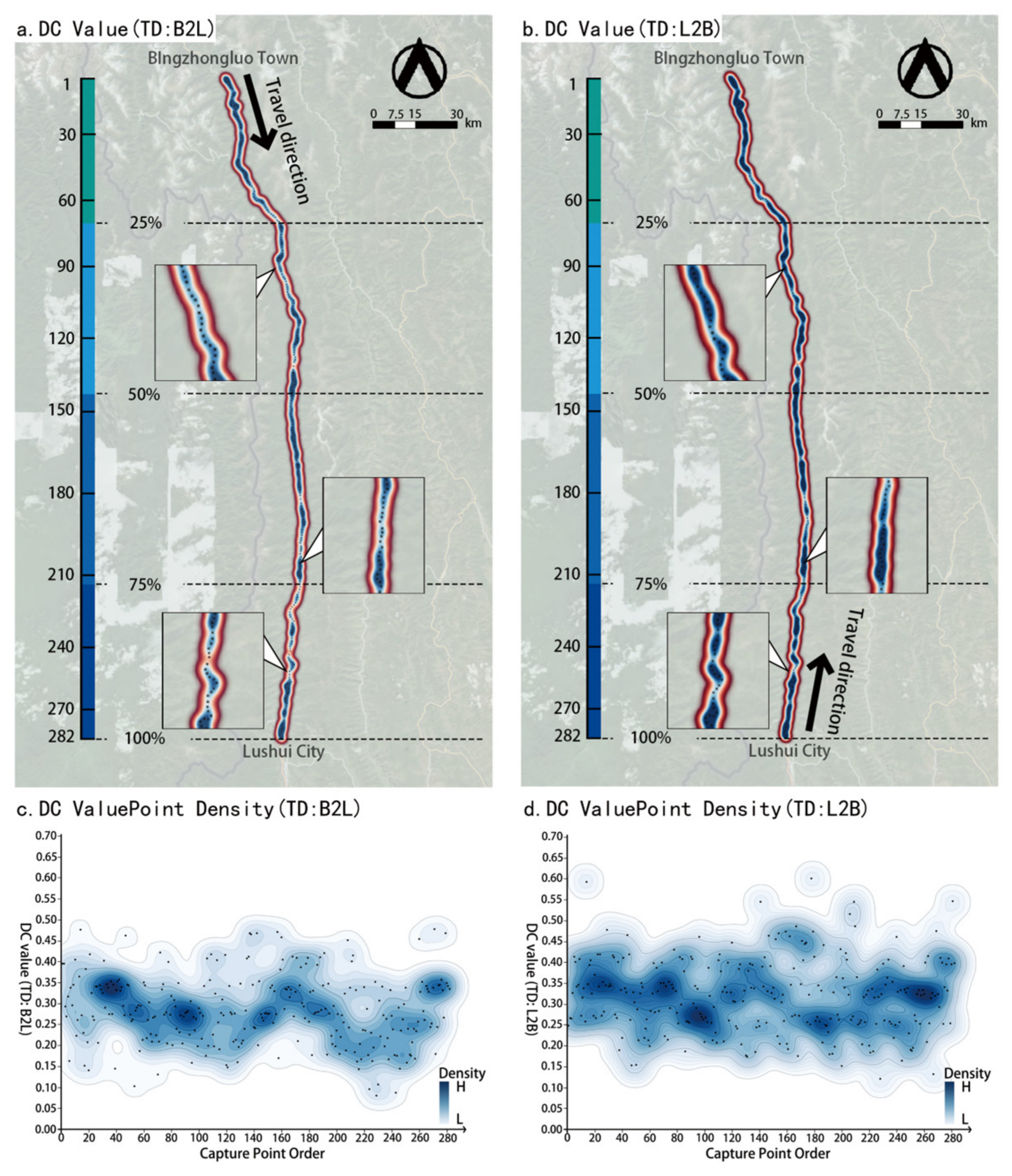
The DC characteristics of the Nujiang Beautiful Road demonstrate significant synchronized changes in both driving directions, exhibiting a rhythmic pattern of “unity–diversity–unity–diversity–unity”. This pattern is evident as alternating light and dark areas in the heatmap (Figure 5), with the point density map also revealing notable fluctuations, indicative of landscape fragmentation. This fragmentation arises from the dispersed distribution of settlements along the route. When dividing the road into four quartile sections, DC values consistently remain higher in the L2B direction than in the B2L direction. This discrepancy is attributed to the proximity of the L2B side to the Nujiang River, where more frequent views of water bodies are available and the open sightlines enable the observation of more landscapes. Conversely, the B2L side’s proximity to the steep mountains of the Nujiang Canyon restricts visibility, particularly around road turns. Furthermore, the prevalence of mountain views on the B2L side reinforces the cohesive nature of the mountain-dominated landscapes.

3.4. OD Evaluation

The OD evaluation results (Table 4) indicate that the OD index of the Nujiang Beautiful Road is 0.6407, suggesting a semi-open spatial characteristic. As the road sections are generally wide with lighter traffic, the road occupies an average of 38% of the visual field, while the sky accounts for only 0.2388 and 0.2735, mainly due to the presence of cliffs. Overall, both directions demonstrate a transition from enclosed to open spaces, with sections nearer to Lushui City being more open. However, this shift at the road section level is relatively minor.
While the changes in OD at the road section level may not be substantial, the density map of OD reveals more dispersed points compared to the density maps of NA and DC (Figure 6). This suggests that although the overall OD experience remains stable, local variations may be more pronounced, thereby enhancing the spatial interest of the driving experience. Furthermore, the difference in OD experience between the two sides of the Nujiang Beautiful Road is more significant compared to differences between sections, with a mean difference of 0.0384. Statistical analysis of OD values using kurtosis reveals that the OD values in the B2L direction are relatively scattered, with a kurtosis of only 2.9108, while the kurtosis in the L2B direction is 4.0425. This indicates that the OD changes in the B2L direction are much more dramatic than those in the L2B direction. This conclusion is also evident in the point density plot. This is because the B2L side is always close to the mountains, and every turn and undulation of the mountain road during the driving process leads to more sensitive OD changes.

3.5. Characteristics of Extreme Value

Observing the landscape element characteristics at the extremum points of three indicators (Figure 7), the following observations can be made:
The NA value serves as an indicator of the landscape matrix. The highest NA value corresponds to the natural landscape matrix, namely the mountain gorge and forest landscape, while the lowest NA value corresponds to the artificial landscape matrix, namely, the settlement landscape. It is important to note that the settlements are essential for sustaining life. If designed thoughtfully, they can also contribute to the cultural landscape. However, the buildings along the Nujiang Beautiful Road are relatively large in scale and do not harmonize well with the surrounding scenery, appearing somewhat incongruous, thus creating a disconnection between the two types of landscape bases. Nevertheless, these structures are primarily apartment buildings constructed to support poverty alleviation efforts, with the larger scale aimed at accommodating more residents, albeit at the expense of aesthetics. It is believed that after the Beautiful Road boosts the regional tourism economy, the appearance will be improved.
Low DC values indicate shifts in landscape themes. Landscape thematicity necessitates a limited number of landscape elements in the field of view. Earlier, we mentioned the concept of “key visual stimulus factors”, which are typically artificial elements. However, this does not imply synchronous changes between DC and NA values. In environments with very low NA values, the DC value may also be low due to the scarcity of natural elements. Along the Nujiang Beautiful Road, low DC values are often manifested in transition zones between urban settlements and natural wilderness, where both natural and artificial elements coexist, resulting in a lack of dominance and a more disorderly appearance. As a validation, among the 144 points (over one-fourth of the total) along the Nujiang Beautiful Road that passed through villages, the road section with more village crossings (25–50%) exhibited a DC standard deviation of 0.0901, while the road section with fewer village crossings (0–25%) had a DC standard deviation of 0.0789. Although this validation method is relatively simplistic, it demonstrates that transitions between natural and artificial themes contribute to fluctuations in the DC value.
Mountains are the key factor influencing the OD value. Since the road area remains relatively constant, the size of the sky area directly reflects the magnitude of the OD value. Upon observing images with the highest and lowest OD values, it becomes evident that scenes with high OD index values feature horizons close to the horizontal line, while scenes with low OD values exhibit sky shapes resembling a “funnel”. Among the landscape elements on both sides of the road, trees, mountains, and buildings are vertical, making them key landscape elements that obstruct sightlines. Pearson correlation tests between the OD value and the proportions of the above three elements reveal that: (a) There exists a strong negative correlation between mountains on both sides of the Nujiang Beautiful Road and the OD value. (b) In the B2L direction, closer to the mountains, the correlation of mountains is stronger than that of trees, whereas in the L2B direction, farther from the mountains, the negative correlation of trees with OD is more pronounced. (c) Interestingly, on the Nujiang Beautiful Road, buildings show a positive correlation with OD. This is because buildings are often situated in relatively flat areas, and their presence does not contribute to openness but rather results from the absence of mountains (Table 5).

3.6. 3D Index Cube: Comprehensive Analysis of SRVLE

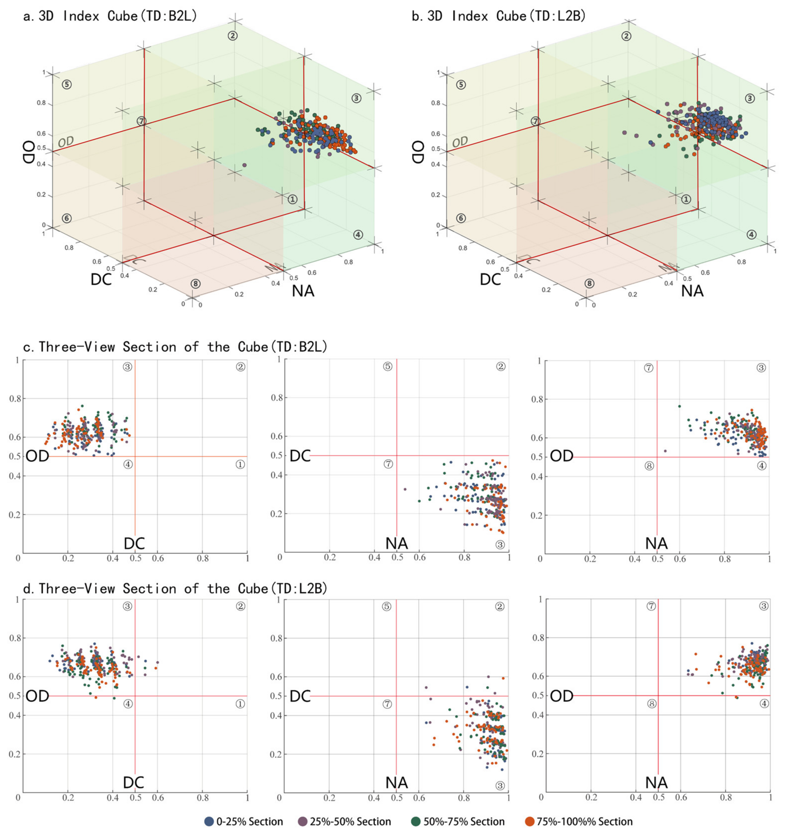
Among the three indicators mentioned above, 1 and 0 represent the two extreme values of the semantic differential concept, with 0.5 serving as the dividing point between the two concepts. If we represent this evaluation system with a 3D index cube, the visual landscape quality of the scenic road can be divided into eight octants, each representing a different combination of landscape characteristics: ① Naturalness–Diversity–Openness; ② Naturalness–Diversity–Deepness; ③ Naturalness–Coherence–Openness; ④ Naturalness–Coherence–Deepness; ⑤ Artificiality–Diversity–Openness; ⑥ Artificiality–Diversity–Deepness; ⑦ Artificiality–Coherence–Openness; and ⑧ Artificiality–Coherence–Openness. By expressing the SRVLE of the case with a 3D index cube, each point accurately expresses the visual quality at this shooting point. This method enables a scientific and intuitive representation of the overall visual landscape quality of the scenic road, which is valuable for formulating relevant planning strategies.
For the Nujiang Beautiful Road case, the visual landscape quality of this scenic road exhibits the following characteristics (Figure 8):
Overall, the three-dimensional semantic evaluation of the Nujiang Beautiful Road indicates that most scatter points are concentrated in the third octant, with a few scattered points in the fourth quadrant (Naturalness—Coherence—Deepness) and the first quadrant (Naturalness—Diversity—Openness). A small number of shooting points passed through settlements, with NA values ranging between 0.50 and 0.80, while the vast majority of scatter points were concentrated in the 0.80–1.00 range. The OD values were mostly distributed between 0.60 and 0.80, with a few points between 0.45 and 0.60, demonstrating a semi-open characteristic. The DC values were mostly between 0.15 and 0.50, with a few points above 0.50. Overall, the visual landscape characteristics of the Nujiang Beautiful Road are relatively rich, with a dominant emphasis on naturalness, coherence, and openness, while some sections exhibit relatively deep and diverse landscapes.
Regarding road sections, the disparities in landscape semantic scatter distribution along the Nujiang Beautiful Road are not substantial. Comparatively, the landscape characteristics of the initial and final sections of the road are deeper and more cohesive, while those of the middle sections are opposite. This is primarily because the middle sections traverse Fugong County and Gongshan County, where the surrounding villages near the county towns are relatively dense. Nonetheless, the scatter points are relatively dispersed regardless of whether they are located in the starting, ending, or middle sections of the road. Overall, the continuity of the road landscape along the Nujiang Beautiful Road is not particularly strong, and the roadside landscape is affected by settlements, resulting in a fragmented road landscape.
When comparing the two driving directions, the scatter points on the B2L side are more clustered, exhibiting a narrower range of fluctuations in the three indicators and fewer changes in the visual landscape. Conversely, the scatter points on the L2B side are relatively dispersed, with the minimum value of the OD indicator and the maximum values of the three indicators all distributed on this side, indicating a higher level of variability in this direction. Overall, the visual landscape of the L2B direction appears to be more natural, diverse, and open compared to the opposite side.

4. Discussion

4.1. Contributions of in Practice

In Western countries where scenic road construction began earlier, relevant laws and regulations already include landscape quality considerations within their management scope. However, achieving a balance between humanistic values and objective standards has always been a challenge. The new method proposed in this study solves this problem to a certain extent.
At the landscape design level, the new method offers a human-scale perspective on road landscape characteristics, enabling the development of more comprehensive and detailed design strategies. Examples include the following: (a) Determining ecological restoration sites: The Nujiang Beautiful Road, being a mountainous scenic road, is vulnerable to soil erosion. Among our 560 visual field images, 123 identified the “bare soil” element, highlighting the significance of fine-grained visual field evaluation for identifying small-scale ecological damage areas. (b) Selecting viewpoint locations: Indicators can pinpoint high- or low-quality landscapes. Locations with high NA and OD values may be suitable for viewpoints. (c) Managing landscape changes: Intense OD value changes along the Nujiang Beautiful Road suggest uncontrolled spatial changes due to natural road vegetation and lack of management, resulting in irregular spatial shifts and abrupt changes that may unsettle drivers [70]. Therefore, employing vegetation to create open and enclosed spaces is essential. (d) Creating segmented themes: Dividing road landscape themes into sections, akin to characteristic zones in scenic areas, enriches and deepens the overall road theme without diminishing its character. (e) Differentiated creation of landscape in both directions: The Nujiang Beautiful Road is situated on the west side of the Nujiang River, causing the B2L direction to be close to the mountains throughout and lacking a view of the water body, resulting in a more oppressive driving experience. Using bridges and roads to connect the opposite side of the canyon could interchange landscape features between directions in specific sections, enhancing the overall landscape experience and offering a comprehensive portrayal of the Nujiang Canyon’s landscape characteristics.
At the environmental management level, scenic road management agencies can utilize this method to conduct statistical analysis of the overall level of road visual landscape quality. They can accurately identify road sections requiring targeted rectification measures based on data’s high, low, and abnormal values. Additionally, by implementing regular image collection and analysis, management agencies can achieve dynamic monitoring of scenic road visual landscape quality. This enables evaluation of road landscape conservation effectiveness and assessment of whether expected planning goals have been met.

4.2. Scale Effect of Bidirectional Differences

This study examines the binocular visual field of leisure driving and concludes that landscape differences exist between the two driving directions, B2L and L2B. This suggests that previous methods, such as remote sensing data analysis of land cover and DEM, may have overlooked potential differences in visual landscapes between different driving directions. Previous research indicates that results obtained at finer scales may differ from or even contradict those at larger scales [82]. The study finds that while the three indices for both directions exhibit certain differences, they generally follow similar trends. Therefore, these differences may be obscured at larger scales, resulting in consistent performance. To verify this, we conducted a difference test on data from both driving directions to determine whether they exhibit statistically significant differences. Paired t-tests were performed on indicator values (means) from one, three, five, seven, and ten sampling points (Supplementary Materials Table S1). Except for the OD indicator, changes in p-values for NA and DC indicators generally show an increasing trend as the observation scale expands. This suggests that visual landscape differences between B2L and L2B directions gradually weaken and become nonsignificant. This is because the NA and DC indicators are calculated based on the types and quantities of landscape elements, and the landscape pattern that the two-way roads depend on constrains the range of changes in the two-way roads; therefore, these two indicators maintain consistency in the overall characteristics of the visual landscape of the two-way roads. However, the OD values of the two directions of the Nujiang Beautiful Road did not tend to be consistent at a larger scale, because the B2L side of the road is always closer to the mountains; therefore, the difference in OD values between the two sides remains significant.

4.3. Limitations and Prospects

Despite integrating binocular visual physiology and image segmentation technology to ensure both subjectivity and objectivity in assessing scenic road visual landscape quality, the new method has several limitations that offer insights for future research: (a) While effective for evaluating and managing landscape visual quality on both sides of the scenic road, current image segmentation algorithms are limited to the intuitive perception of the human eye. They cannot reflect a deeper understanding of the landscape by the observer, thus failing to reveal the historical and cultural value behind the visual landscape. For instance, the Nujiang Beautiful Road, surrounded by multiple ethnic minorities, features traditional architecture reflecting unique cultural values that are not captured in the evaluation. (b) The viewer’s perspective may change during leisure driving on the scenic road. Although this study simulates the binocular visual field range assuming a normal driving scenario where the driver looks ahead, it overlooks consideration of the subject’s dynamic visual field, necessitating exploration of appropriate methods.
While this study demonstrates the effectiveness of our method through the case of the Nujiang Beautiful Road, we acknowledge the limitation of relying on a single case study. Future research should extend the application of this method to a broader range of scenic roads, including those in diverse geographical settings (e.g., coastal and prairie) and with varying levels of development and management. Such an expanded application would not only validate the method’s versatility but also potentially uncover how different landscape types influence visual quality indicators. These findings could provide valuable insights for tailoring scenic road planning and management strategies to specific landscape contexts. Although the NA, DC, and OD indicators proposed in this study are universally applicable, they have not been weighted and aggregated to derive a composite score. However, determining weights for specific scenic roads is still of significant importance for evaluating their overall landscape quality. Therefore, future research may consider encouraging scenic road management authorities to develop more refined indicators tailored to specific scenic roads. By integrating the opinions of experts from various fields, the perspectives of local residents, and feedback from motorists, a comprehensive evaluation system can be constructed, leading to more scientifically grounded composite evaluation results. With the advent of the AI era, cross-modal technology may enable image analysis to incorporate cultural significance. Consequently, the visual landscape quality evaluation of scenic roads will evolve towards a more comprehensive, precise, and people-oriented approach, providing better support for the planning, construction, and management of scenic roads and surrounding landscapes.

5. Conclusions

The visual landscape of roads plays a dual role as a foundational resource for scenic road construction and a vital reference for establishing scenic road route systems and integrating transportation and tourism development. To assess the visual landscape resources provided by scenic roads more scientifically and accurately, this paper proposes a new method for measuring the visual landscape quality of scenic roads, exemplified by the Nujiang Beautiful Road in Yunnan. This study tackles both subjectivity and objectivity concerns by leveraging binocular visual field images and image segmentation, achieving SRVLE based on a “non-scale semantic differential approach”. Compared to existing methods, this study effectively integrates the strengths of both public and expert evaluation paradigms while mitigating their respective weaknesses. For the public paradigm, we achieve the following: (a) we enhance subjectivity by simulating the binocular visual field; (b) we eliminate the subjectivity and bias associated with questionnaires and scales. For the expert paradigm, we achieve the following: (a) we maintain spatial analysis and precise measurement, exploring landscape quality’s spatial distribution objectively; (b) we quantify drivers’ visual experiences, addressing the expert paradigm’s focus on land attributes and ignoring human perception. This study validates the effectiveness of the new method based on empirical cases, offering a new approach for evaluating the visual landscape quality of scenic roads.

Supplementary Materials

The following supporting information can be downloaded at: https://www.mdpi.com/article/10.3390/land13091381/s1.

Author Contributions

Z.B.: conceptualization, resources, methodology, software, writing—original draft. R.J.: conceptualization, editing, formal analysis. J.Q.: supervision, editing, funding acquisition, formal analysis. All authors have read and agreed to the published version of the manuscript.

Funding

This work was supported by the National Natural Science Foundation of China under Grant No. 51908477.

Data Availability Statement

The data that support the findings of this study are available from the corresponding author upon reasonable request.

Conflicts of Interest

The authors declare that they have no known competing financial interests or personal relationships that could have appeared to influence the work reported in this paper.

References

  1. Brown, G. A Method for Assessing Highway Qualities to Integrate Values in Highway Planning. J. Transp. Geogr. 2003, 11, 271–283. [Google Scholar] [CrossRef]
  2. Denstadli, J.M.; Jacobsen, J.K.S. The Long and Winding Roads: Perceived Quality of Scenic Tourism Routes. Tour. Manag. 2011, 32, 780–789. [Google Scholar] [CrossRef]
  3. Clay, G.R.; Smidt, R.K. Assessing the Validity and Reliability of Descriptor Variables Used in Scenic Highway Analysis. Landsc. Urban Plan. 2004, 66, 239–255. [Google Scholar] [CrossRef]
  4. Eliot, C.W. The Influence of the Automobile on the Design of Park Roads. Landsc. Archit. 1922, 13, 27–37. [Google Scholar]
  5. Bilberman, J.; Andereck, K.L. The Economic Value of Off-Highway Vehicle Recreation. J. Leis. Res. 2006, 38, 208–223. [Google Scholar] [CrossRef]
  6. Yang, X.; Yue, F.; Liu, Y.; Fan, P. Research on Evaluation Ideas and Index Construction of China’s Scenic Byway. In Proceedings of the International Conference on Frontiers of Traffic and Transportation Engineering (FTTE 2022), Lanzhou, China, 17–19 June 2022. [Google Scholar]
  7. Zhang, Y.; Chen, X.; Yu, R.; Cheng, J.; Yu, X. The Logic Transformation of the Scenic Byway System to the Linear Experience Space Transformation. J. Nat. Resour. 2020, 35, 284–296. [Google Scholar] [CrossRef]
  8. Zhang, J.; Zhang, Y. Tourism, Transport Infrastructure and Income Inequality: A Panel Data Analysis of China. Curr. Issues Tour. 2022, 25, 1607–1626. [Google Scholar] [CrossRef]
  9. Qin, X.; Fang, M.; Yang, D.; Wangari, V.W. Quantitative Evaluation of Attraction Intensity of Highway Landscape Visual Elements Based on Dynamic Perception. Environ. Impact Assess. Rev. 2023, 100, 107081. [Google Scholar] [CrossRef]
  10. Steenjacobsen, J.K. Nomadic Tourism and Fleeting Place Encounters: Exploring Different Aspects of Sightseeing. Scand. J. Hosp. Tour. 2001, 1, 99–112. [Google Scholar] [CrossRef]
  11. Jiang, L.; Kang, J.; Schroth, O. Prediction of the Visual Impact of Motorways Using GIS. Environ. Impact Assess. Rev. 2015, 55, 59–73. [Google Scholar] [CrossRef]
  12. Kang, N.; Liu, C. Towards Landscape Visual Quality Evaluation: Methodologies, Technologies, and Recommendations. Ecol. Indic. 2022, 142, 109174. [Google Scholar] [CrossRef]
  13. Tveit, M.; Ode, Å.; Fry, G. Key Concepts in a Framework for Analysing Visual Landscape Character. Landsc. Res. 2006, 31, 229–255. [Google Scholar] [CrossRef]
  14. Daniel, T.C. Whither Scenic Beauty? Visual Landscape Quality Assessment in the 21st Century. Landsc. Urban Plan. 2001, 54, 267–281. [Google Scholar] [CrossRef]
  15. Howley, P. Landscape Aesthetics: Assessing the General Publics’ Preferences towards Rural Landscapes. Ecol. Econ. 2011, 72, 161–169. [Google Scholar] [CrossRef]
  16. Palmer, J.F. A Diversity of Approaches to Visual Impact Assessment. Land 2022, 11, 1006. [Google Scholar] [CrossRef]
  17. Kent, R.L.; Elliott, C.L. Scenic Routes Linking and Protecting Natural and Cultural Landscape Features: A Greenway Skeleton. Landsc. Urban Plan. 1995, 33, 341–355. [Google Scholar] [CrossRef]
  18. Solecka, I. The Use of Landscape Value Assessment in Spatial Planning and Sustainable Land Management—A Review. Landsc. Res. 2019, 44, 966–981. [Google Scholar] [CrossRef]
  19. Sipes, J.L.; James, A.P.; Lindley, J.; Campbell, T.; Gragg, R.; Harbert, C. Scenic Byways: A Review of Processes, Administration, and Economic Impacts. Transp. Res. Rec. 1997, 1599, 96–103. [Google Scholar] [CrossRef]
  20. Zhu, G.; Zhong, P.; Luo, Y.; Yan, L.; Yang, D.; Long, W. Highway Landscape Planning Based on “3S” Technologies—Taking the Sichuan-Tibet Highway (Kanding Section) as an Example. 2015, pp. 2787–2798. Available online: https://ascelibrary.org/doi/abs/10.1061/9780784479384.356 (accessed on 13 June 2024).
  21. Palmer, J.F.; Hoffman, R.E. Rating Reliability and Representation Validity in Scenic Landscape Assessments. Landsc. Urban Plan. 2001, 54, 149–161. [Google Scholar] [CrossRef]
  22. Otero Pastor, I.; Casermeiro Martínez, M.A.; Ezquerra Canalejoa, A.; Esparcia Mariño, P. Landscape Evaluation: Comparison of Evaluation Methods in a Region of Spain. J. Environ. Manag. 2007, 85, 204–214. [Google Scholar] [CrossRef]
  23. Crawford, D. Using Remotely Sensed Data in Landscape Visual Quality Assessment. Landsc. Urban Plan. 1994, 30, 71–81. [Google Scholar] [CrossRef]
  24. Sahle, M.; Saito, O. Mapping and Characterizing the Jefoure Roads That Have Cultural Heritage Values in the Gurage Socio-Ecological Production Landscape of Ethiopia. Landsc. Urban Plan. 2021, 210, 104078. [Google Scholar] [CrossRef]
  25. Martín, B.; Ortega, E.; Otero, I.; Arce, R.M. Landscape Character Assessment with GIS Using Map-Based Indicators and Photographs in the Relationship between Landscape and Roads. J. Environ. Manag. 2016, 180, 324–334. [Google Scholar] [CrossRef]
  26. Anderson, C.C.; Rex, A. Preserving the Scenic Views from North Carolina’s Blue Ridge Parkway: A Decision Support System for Strategic Land Conservation Planning. Appl. Geogr. 2019, 104, 75–82. [Google Scholar] [CrossRef]
  27. Palmer, J.F. The Contribution of a GIS-Based Landscape Assessment Model to a Scientifically Rigorous Approach to Visual Impact Assessment. Landsc. Urban Plan. 2019, 189, 80–90. [Google Scholar] [CrossRef]
  28. Blumentrath, C.; Tveit, M.S. Visual Characteristics of Roads: A Literature Review of People’s Perception and Norwegian Design Practice. Transp. Res. Part Policy Pract. 2014, 59, 58–71. [Google Scholar] [CrossRef]
  29. Hunziker, M.; Felber, P.; Gehring, K.; Buchecker, M.; Bauer, N.; Kienast, F. Evaluation of Landscape Change by Different Social Groups. Mt. Res. Dev. 2008, 28, 140–147. [Google Scholar] [CrossRef]
  30. Scott, A. Assessing Public Perception of Landscape: The LANDMAP Experience. Landsc. Res. 2002, 27, 271–295. [Google Scholar] [CrossRef]
  31. Frank, S.; Fürst, C.; Koschke, L.; Witt, A.; Makeschin, F. Assessment of Landscape Aesthetics—Validation of a Landscape Metrics-Based Assessment by Visual Estimation of the Scenic Beauty. Ecol. Indic. 2013, 32, 222–231. [Google Scholar] [CrossRef]
  32. Ribe, R. Exploring Psychophysical Measurement in Landscape Aesthetics: Validity, Reliability and Signal Detection via Single-versus Opposing-Construct Rating Scales, with or without Zeros. J. Environ. Psychol. 2022, 83, 101862. [Google Scholar] [CrossRef]
  33. Matijošaitienė, I.; Stankevičė, I. Road Landscape as a Product: Does It Satisfy Consumers’ Aesthetic Needs? Balt. J. Road Bridge Eng. 2014, 9, 297–305. [Google Scholar] [CrossRef]
  34. Symonds, P.M. On the Loss of Reliability in Ratings Due to Coarseness of the Scale. J. Exp. Psychol. 1924, 7, 456–461. [Google Scholar] [CrossRef]
  35. Terkenli, T.S.; Gkoltsiou, A.; Kavroudakis, D. The Interplay of Objectivity and Subjectivity in Landscape Character Assessment: Qualitative and Quantitative Approaches and Challenges. Land 2021, 10, 53. [Google Scholar] [CrossRef]
  36. Biljecki, F.; Ito, K. Street View Imagery in Urban Analytics and GIS: A Review. Landsc. Urban Plan. 2021, 215, 104217. [Google Scholar] [CrossRef]
  37. Ma, X.; Ma, C.; Wu, C.; Xi, Y.; Yang, R.; Peng, N.; Zhang, C.; Ren, F. Measuring Human Perceptions of Streetscapes to Better Inform Urban Renewal: A Perspective of Scene Semantic Parsing. Cities 2021, 110, 103086. [Google Scholar] [CrossRef]
  38. Steen Jacobsen, J.K. Use of Landscape Perception Methods in Tourism Studies: A Review of Photo-Based Research Approaches. Tour. Geogr. 2007, 9, 234–253. [Google Scholar] [CrossRef]
  39. Banks, M.S.; Cooper, E.A.; Piazza, E.A. Camera Focal Length and the Perception of Pictures. Ecol. Psychol. 2014, 26, 30–46. [Google Scholar] [CrossRef]
  40. Cooper, E.A.; Piazza, E.A.; Banks, M.S. The Perceptual Basis of Common Photographic Practice. J. Vis. 2012, 12, 8. [Google Scholar] [CrossRef]
  41. Hammitt, W.E.; Patterson, M.E.; Noe, F.P. Identifying and Predicting Visual Preference of Southern Appalachian Forest Recreation Vistas. Landsc. Urban Plan. 1994, 29, 171–183. [Google Scholar] [CrossRef]
  42. Sevenant, M.; Antrop, M. Landscape Representation Validity: A Comparison between On-Site Observations and Photographs with Different Angles of View. Landsc. Res. 2011, 36, 363–385. [Google Scholar] [CrossRef]
  43. Stewart, T.R.; Middleton, P.; Downton, M.; Ely, D. Judgments of Photographs vs. Field Observations in Studies of Perception and Judgment of the Visual Environment. J. Environ. Psychol. 1984, 4, 283–302. [Google Scholar] [CrossRef]
  44. Xiang, Y.; Liang, H.; Fang, X.; Chen, Y.; Xu, N.; Hu, M.; Chen, Q.; Mu, S.; Hedblom, M.; Qiu, L.; et al. The Comparisons of On-Site and off-Site Applications in Surveys on Perception of and Preference for Urban Green Spaces: Which Approach Is More Reliable? Urban For. Urban Green. 2021, 58, 126961. [Google Scholar] [CrossRef]
  45. Chen, G.; Yan, J.; Wang, C.; Chen, S. Expanding the Associations between Landscape Characteristics and Aesthetic Sensory Perception for Traditional Village Public Space. Forests 2024, 15, 97. [Google Scholar] [CrossRef]
  46. Li, X.; Wang, X.; Jiang, X.; Han, J.; Wang, Z.; Wu, D.; Lin, Q.; Li, L.; Zhang, S.; Dong, Y. Prediction of Riverside Greenway Landscape Aesthetic Quality of Urban Canalized Rivers Using Environmental Modeling. J. Clean. Prod. 2022, 367, 133066. [Google Scholar] [CrossRef]
  47. Long, K.; Wang, N.; Lin, Z. Assessing Scenic Beauty of Hilly and Mountain Villages: An Approach Based on Landscape Indicators. Ecol. Indic. 2023, 154, 110538. [Google Scholar] [CrossRef]
  48. Guan, F.; Fang, Z.; Wang, L.; Zhang, X.; Zhong, H.; Huang, H. Modelling People’s Perceived Scene Complexity of Real-World Environments Using Street-View Panoramas and Open Geodata. ISPRS J. Photogramm. Remote Sens. 2022, 186, 315–331. [Google Scholar] [CrossRef]
  49. Li, Y.; Yabuki, N.; Fukuda, T. Measuring Visual Walkability Perception Using Panoramic Street View Images, Virtual Reality, and Deep Learning. Sustain. Cities Soc. 2022, 86, 104140. [Google Scholar] [CrossRef]
  50. Gao, S.; Yang, K.; Shi, H.; Wang, K.; Bai, J. Review on Panoramic Imaging and Its Applications in Scene Understanding. IEEE Trans. Instrum. Meas. 2022, 71, 1–34. [Google Scholar] [CrossRef]
  51. Pardo-García, S.; Mérida-Rodríguez, M. Measurement of Visual Parameters of Landscape Using Projections of Photographs in GIS. Comput. Environ. Urban Syst. 2017, 61, 56–65. [Google Scholar] [CrossRef]
  52. Kang, Y.; Kim, J.; Park, J.; Lee, J. Assessment of Perceived and Physical Walkability Using Street View Images and Deep Learning Technology. ISPRS Int. J. Geo-Inf. 2023, 12, 186. [Google Scholar] [CrossRef]
  53. Gandy, R.; Meitner, M.J. The Effects of an Advanced Traveler Information System on Scenic Beauty Ratings and the Enjoyment of a Recreational Drive. Landsc. Urban Plan. 2007, 82, 85–93. [Google Scholar] [CrossRef]
  54. Portman, M.E.; Natapov, A.; Fisher-Gewirtzman, D. To Go Where No Man Has Gone before: Virtual Reality in Architecture, Landscape Architecture and Environmental Planning. Comput. Environ. Urban Syst. 2015, 54, 376–384. [Google Scholar] [CrossRef]
  55. Qi, J.; Tang, X. Interacting with Landscapes beyond the Windshield: Affordances Actualisation on Scenic Road Rest Areas along the Nujiang Beautiful Road in China. Landsc. Res. 2024, 49, 1–17. [Google Scholar] [CrossRef]
  56. Guitton, D.; Volle, M. Gaze Control in Humans: Eye-Head Coordination during Orienting Movements to Targets within and beyond the Oculomotor Range. J. Neurophysiol. 1987, 58, 427–459. [Google Scholar] [CrossRef]
  57. Yao, X.; Toslak, D.; Son, T.; Ma, J. Understanding the Relationship between Visual-Angle and Eye-Angle for Reliable Determination of the Field-of-View in Ultra-Wide Field Fundus Photography. Biomed. Opt. Express 2021, 12, 6651–6659. [Google Scholar] [CrossRef] [PubMed]
  58. Ruch, T.C.; Fulton, J.F. Medical Physiology and Biophysics. Acad. Med. 1960, 35, 1067. [Google Scholar]
  59. Jiang, J.; Brack, C.; Coe, R.; Gibbons, P. Rapidly Quantifying Interior Greenery Using 360° Panoramic Images. Forests 2022, 13, 602. [Google Scholar] [CrossRef]
  60. Jo, H.I.; Jeon, J.Y. Overall Environmental Assessment in Urban Parks: Modelling Audio-Visual Interaction with a Structural Equation Model Based on Soundscape and Landscape Indices. Build. Environ. 2021, 204, 108166. [Google Scholar] [CrossRef]
  61. Guiducci, D.; Burke, A. Reading the Landscape: Legible Environments and Hominin Dispersals. Evol. Anthropol. Issues News Rev. 2016, 25, 133–141. [Google Scholar] [CrossRef]
  62. Ogburn, D.E. Assessing the Level of Visibility of Cultural Objects in Past Landscapes. J. Archaeol. Sci. 2006, 33, 405–413. [Google Scholar] [CrossRef]
  63. Guo, J.; He, H.; He, T.; Lausen, L.; Li, M.; Lin, H.; Shi, X.; Wang, C.; Xie, J.; Zha, S.; et al. GluonCV and GluonNLP: Deep Learning in Computer Vision and Natural Language Processing. J. Mach. Learn. Res. 2020, 21, 1–7. [Google Scholar]
  64. Zhu, J.; Li, B.; Ouyang, H.; Wang, Y.; Bai, Z. Understanding Urban Residents’ Walking Exercise Preferences: An Empirical Study Using Street View Images and Trajectory Data. Buildings 2024, 14, 549. [Google Scholar] [CrossRef]
  65. Ode, Å.; Tveit, M.S.; Fry, G. Advantages of Using Different Data Sources in Assessment of Landscape Change and Its Effect on Visual Scale. Ecol. Indic. 2010, 10, 24–31. [Google Scholar] [CrossRef]
  66. Smardon, R.C. Visual Impact Assessment: Where Have We Come from and Where Are We Going? J. Environ. Prot. 2016, 7, 1333–1341. [Google Scholar] [CrossRef]
  67. Farber, M.E.; Hall, T.E. Emotion and Environment: Visitors’ Extraordinary Experiences along the Dalton Highway in Alaska. J. Leis. Res. 2007, 39, 248–270. [Google Scholar] [CrossRef]
  68. Mehmetoglu, M.; Normann, Ø. The Link between Travel Motives and Activities in Nature-based Tourism. Tour. Rev. 2013, 68, 3–13. [Google Scholar] [CrossRef]
  69. Carver, S.; Comber, A.; McMorran, R.; Nutter, S. A GIS Model for Mapping Spatial Patterns and Distribution of Wild Land in Scotland. Landsc. Urban Plan. 2012, 104, 395–409. [Google Scholar] [CrossRef]
  70. Thiffault, P.; Bergeron, J. Monotony of Road Environment and Driver Fatigue: A Simulator Study. Accid. Anal. Prev. 2003, 35, 381–391. [Google Scholar] [CrossRef] [PubMed]
  71. Liu, L.; Gao, Z.; Luo, P.; Duan, W.; Hu, M.; Mohd Arif Zainol, M.R.R.; Zawawi, M.H. The Influence of Visual Landscapes on Road Traffic Safety: An Assessment Using Remote Sensing and Deep Learning. Remote Sens. 2023, 15, 4437. [Google Scholar] [CrossRef]
  72. Yue, Z.; Zhong, Y.; Cui, Z. Respondent Dynamic Attention to Streetscape Composition in Nanjing, China. Sustainability 2022, 14, 15209. [Google Scholar] [CrossRef]
  73. Zhao, J.; Wu, J.; Wang, H. Characteristics of Urban Streets in Relation to Perceived Restorativeness. J. Expo. Sci. Environ. Epidemiol. 2020, 30, 309–319. [Google Scholar] [CrossRef]
  74. Antrop, M.; Van Eetvelde, V. Holistic Aspects of Suburban Landscapes: Visual Image Interpretation and Landscape Metrics. Landsc. Urban Plan. 2000, 50, 43–58. [Google Scholar] [CrossRef]
  75. Stamps, A.E., III. Entropy, Visual Diversity, and Preference. J. Gen. Psychol. 2002, 129, 300–320. [Google Scholar] [CrossRef] [PubMed]
  76. Jost, L. Entropy and Diversity. Oikos 2006, 113, 363–375. [Google Scholar] [CrossRef]
  77. Rocchini, D.; Delucchi, L.; Bacaro, G.; Cavallini, P.; Feilhauer, H.; Foody, G.M.; He, K.S.; Nagendra, H.; Porta, C.; Ricotta, C.; et al. Calculating Landscape Diversity with Information-Theory Based Indices: A GRASS GIS Solution. Ecol. Inform. 2013, 17, 82–93. [Google Scholar] [CrossRef]
  78. Juhász-Nagy, P. Notes on Compositional Diversity. In Proceedings of the Intermediate Disturbance Hypothesis in Phytoplankton Ecology; Padisák, J., Reynolds, C.S., Sommer, U., Eds.; Springer: Dordrecht, The Netherlands, 1993; pp. 173–182. [Google Scholar]
  79. Konrád, K.D.; Bede-Fazekas, Á.; Bartha, S.; Somodi, I. Adapting a Multiscale Approach to Assess the Compositional Diversity of Landscapes. Landsc. Ecol. 2023, 38, 2731–2747. [Google Scholar] [CrossRef]
  80. Han, X.; Wang, L.; Seo, S.H.; He, J.; Jung, T. Measuring Perceived Psychological Stress in Urban Built Environments Using Google Street View and Deep Learning. Front. Public Health 2022, 10, 891736. [Google Scholar] [CrossRef]
  81. Yu, X.; Ma, J.; Tang, Y.; Yang, T.; Jiang, F. Can We Trust Our Eyes? Interpreting the Misperception of Road Safety from Street View Images and Deep Learning. Accid. Anal. Prev. 2024, 197, 107455. [Google Scholar] [CrossRef]
  82. Turner, M.G.; O’Neill, R.V.; Gardner, R.H.; Milne, B.T. Effects of Changing Spatial Scale on the Analysis of Landscape Pattern. Landsc. Ecol. 1989, 3, 153–162. [Google Scholar] [CrossRef]
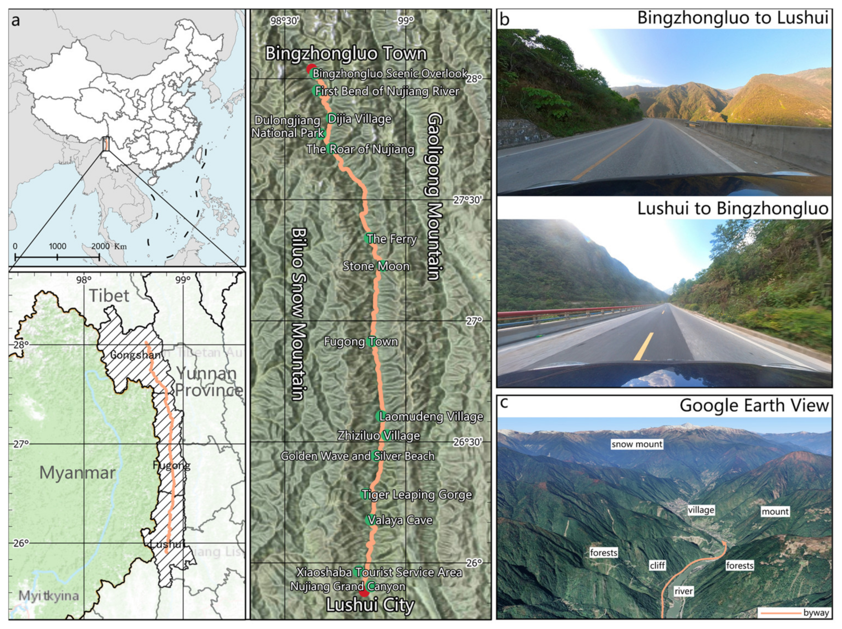
Figure 1. Overview map of the study area. (a) Geographic location of the study area. (b) Actual image of the Nujiang Beautiful Road. (c) Three-dimensional terrain image of the Nujiang Beautiful Road.
Land 13 01381 g001
Figure 2. Process for obtaining human visual field images. Acquisition methods, acquisition equipment, visual field simulation, and image segmentation.
Land 13 01381 g002
Figure 3. Examples of sampling scenes. The red dots on the map are arranged at 20 km intervals.
Land 13 01381 g003
Figure 4. Spatial distribution and density of NA index. (a) NA heatmap of B2L direction, (b) NA heatmap of L2B direction, (c) NA point density of B2L direction, and (d) NA point density of L2B direction.
Land 13 01381 g004
Figure 5. Spatial distribution and density of DC index. (a) DC heatmap of B2L direction, (b) DC heatmap of L2B direction, (c) DC point density of B2L direction, and (d) DC point density of L2B direction.
Land 13 01381 g005
Figure 6. Spatial distribution and density of OD index. (a) OD heatmap of B2L direction, (b) OD heatmap of L2B direction, (c) OD point density of B2L direction, and (d) OD point density of L2B direction.
Land 13 01381 g006
Figure 7. Extreme points of the three indexes in this case study.
Land 13 01381 g007
Figure 8. Three-dimensional index cube. (a) Three-dimensional index cube for the B2L direction, (b) 3D index cube for the L2B direction, (c) three-view section of the cube for the B2L direction, and (d) three-view section of the cube for the L2B direction.
Land 13 01381 g008
Table 1. Semantic segmentation results of Nujiang Beautiful Road landscape labels.
LabelB2LL2B
CategoryTypesMin/MaxMeanSDMin/MaxMeanSD
NaturalTree0.0002/0.41090.10150.08700.0000/0.37920.08460.0671
Shrub0.0000/0.11590.00950.01810.0000/0.16800.00830.0130
Mountain0.0001/0.43410.20100.10430.0222/0.49800.18940.0724
Bare land0.0000/0.08310.00380.01190.0000/0.06400.00260.0079
Sky0.1017/0.37250.23880.04720.0778/0.35400.27350.0406
Water0.0000/0.02790.00050.00300.0000/0.07250.00430.0093
ArtificialRoad0.3218/0.44650.38270.01800.3122/0.44370.38630.0241
Building0.0000/0.20960.00820.02590.0000/0.19840.01060.0310
Wall0.0000/0.18300.02600.03310.0000/0.24410.02040.0226
Fence0.0000/0.08530.01030.00950.0000/0.05610.00850.0095
Bridge0.0000/0.00000.00000.00000.0000/0.02150.00010.0013
Sign0.0000/0.04620.00090.00400.0000/0.02220.00060.0026
Pole/tower0.0000/0.05120.00070.00420.0000/0.02460.00060.0031
ExclusionsVehicle0.0000/0.07110.00130.00670.0000/0.03660.00520.0037
Unidentified0.0001/0.05790.01470.01220.0000/0.04770.00950.0063
Table 2. NA index of Nujiang Beautiful Road.
Road DirectionMinMaxMean
Total0–25% Section25–50% Section50–75% Section75–100% Section
B2L0.53660.98970.89940.88940.90420.88160.9228
L2B0.63340.99320.91050.89700.91250.90190.9305
Table 3. DC index of Nujiang Beautiful Road.
Road DirectionElements per
Image (Mean)
Mean
Total0–25% Section25–50% Section50–75% Section75–100% Section
B2L6.25450.28390.29260.27930.30820.2549
L2B6.79290.31980.32670.30810.33750.3057
Table 4. OD index of Nujiang Beautiful Road.
Road DirectionMinMaxMean
Total0–25% Section25–50% Section50–75% Section75–100% Section
B2L0.50510.76160.62150.60360.61760.64310.6213
L2B0.48830.77000.65990.64210.64370.67420.6784
Table 5. Pearson test between OD value and landscape elements.
Road DirectionTreeMountainBuilding
B2L−0.361 **−0.432 **0.253 *
L2B−0.676 **−0.230 *0.257 *
Note: * p < 0.05, ** p < 0.01.
Disclaimer/Publisher’s Note: The statements, opinions and data contained in all publications are solely those of the individual author(s) and contributor(s) and not of MDPI and/or the editor(s). MDPI and/or the editor(s) disclaim responsibility for any injury to people or property resulting from any ideas, methods, instructions or products referred to in the content.