
Meta-Connectivity in Urban Morphology: A Deep Generative Approach for Integrating Human–Wildlife Landscape Connectivity in Urban Design

 ,
,
Abstract
:1. Introduction
1.1. Significance of Landscape Connectivity to Urban Ecology
Cross-Domain Translation and Conditional Design Reasoning
1.2. The Meta-Connectivity Hypothesis
2. Material and Methods
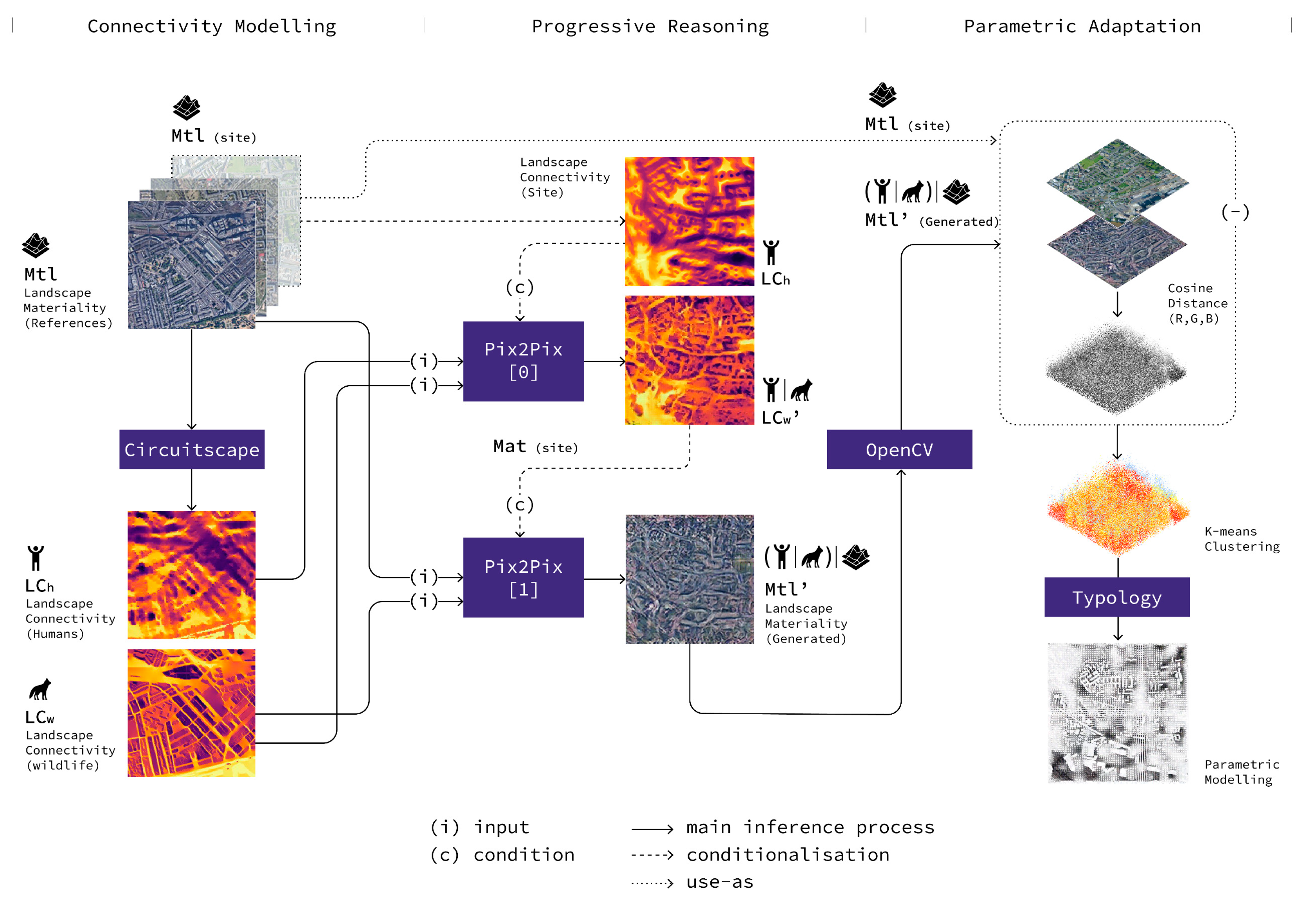
2.1. The Meta-Connectivity Framework
2.2. Study Area
2.3. Data Collection
2.3.1. Landscape Connectivity on NBI Data
2.3.2. Landscape Connectivity on eBird Data
2.4. Modelling Landscape Connectivity
2.5. Analytical Metrics of Dataset Processing
2.6. Dataset Observations
2.6.1. Testing Site
2.6.2. Data Evaluation
2.6.3. Metric Biases
3. Architecture of Reasoning System
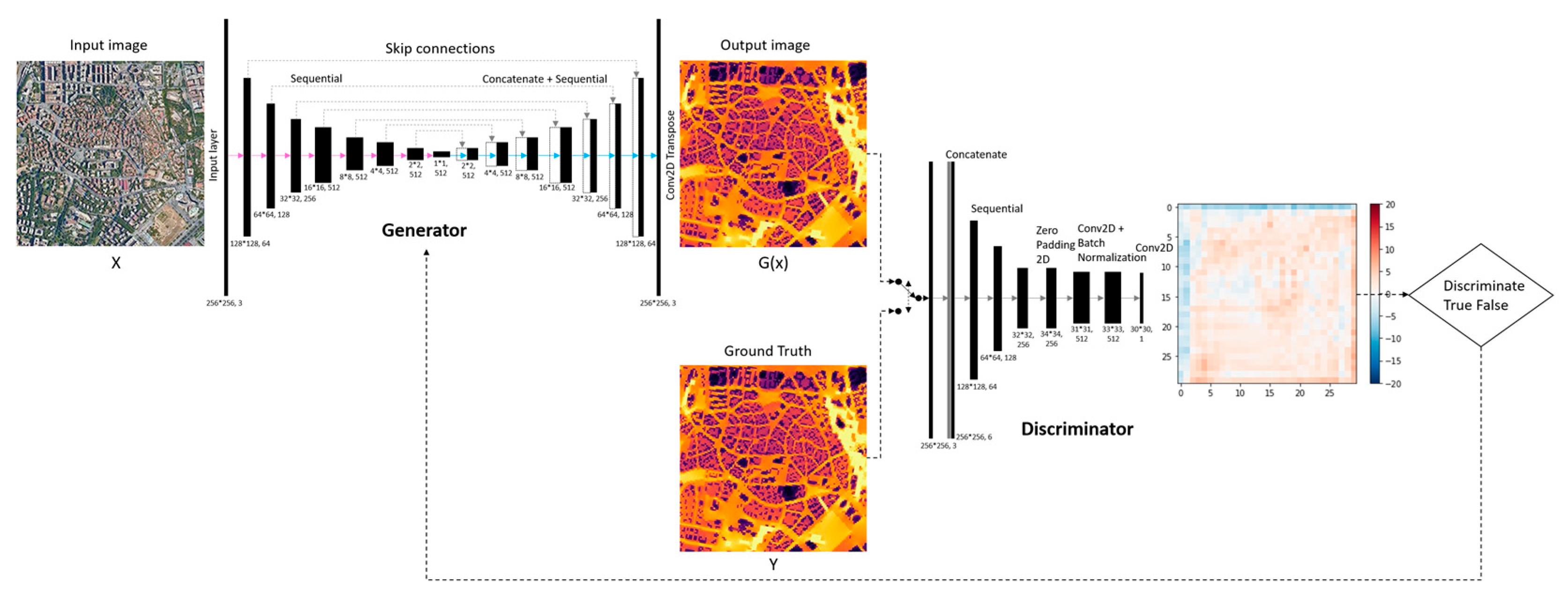
3.1. Conditional Generative Model: Pix2Pix
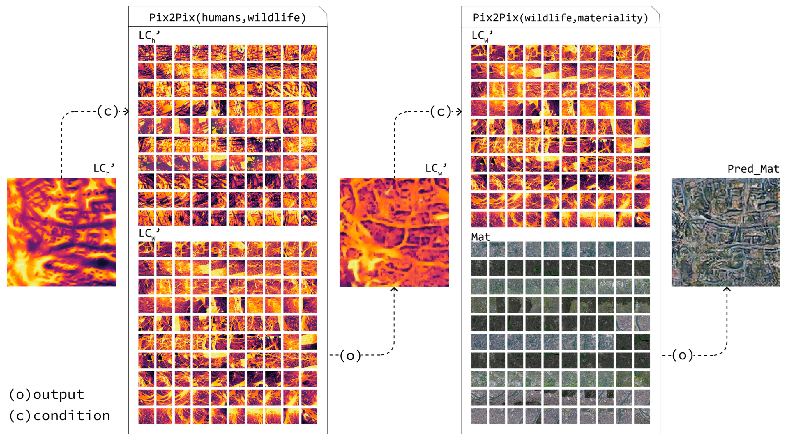
3.2. Progressive Reasoning
3.3. Training Pix2Pix Models
4. Results
4.1. Summary of Results
4.1.1. General Observations
4.1.2. Variational Analysis: Guiding the Urban Design Process
4.2. Reviewing Generated Outputs
4.2.1. General Observation
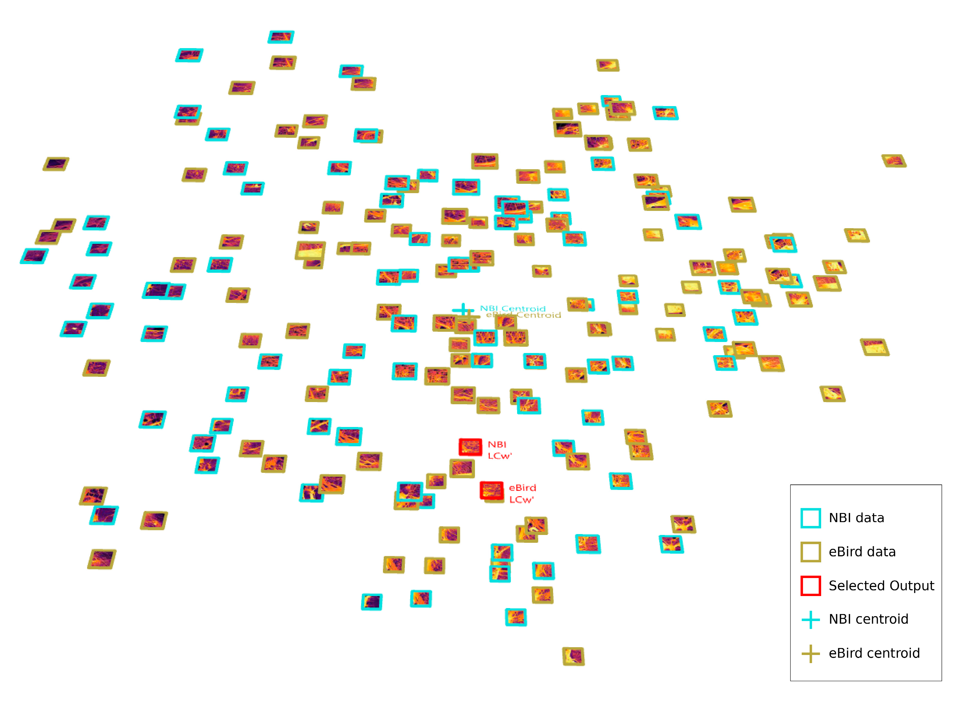
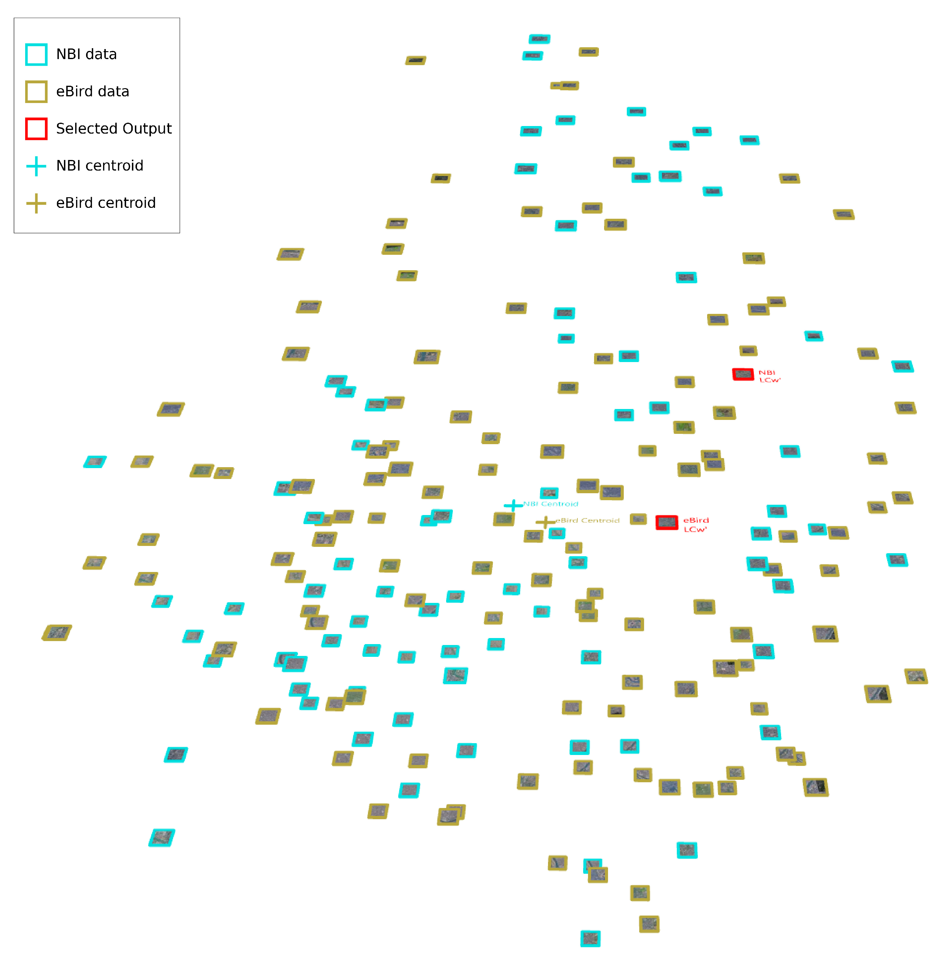
4.2.2. Searching the Best Fit of the Targeted Landscape Connectivity Model
5. Discussion
5.1. Main Findings
5.1.1. Redefining Urban Nature with Meta-Connected Morphology
5.1.2. Latent-Topia: The Meta-Connectivity Revealed by the Datasets
5.1.3. Methodological Subjectivity
5.2. Research Limitations
6. Conclusions
- Integration of Connectivity Metrics: This study successfully integrates human and wildlife connectivity metrics within a single design process. This integration is crucial for creating urban forms that support both human activities and ecological networks. The empirical results from the East London case study validate that the framework can effectively align human and wildlife connectivity, showcasing its practical application. It should be acknowledged that the limitations of the data may result in the findings providing only a limited representation of human–wildlife symbiotic landscape connectivity in a city rather than a general, comprehensive integration.
- Adaptive Design through Gradients: This research highlights the effectiveness of using connectivity gradients rather than traditional corridor-based approaches. The gradient-driven design allows for more flexible and adaptive urban planning, accommodating both human and wildlife needs in a dynamic urban environment. This method was validated through the empirical study, where the framework demonstrated its ability to adjust connectivity based on real-time data.
- Latent Space Similarity in Connectivity Data: This study found that the latent space data distribution between the NBI and eBird connectivity datasets shows a remarkable similarity, indicating that medium to large mammals and birds exhibit comparable spatial connectivity patterns influenced by land factors. This reinforces the framework’s applicability in considering both types of wildlife.
Author Contributions
Funding
Data Availability Statement
Acknowledgments
Conflicts of Interest
Appendix A

| Analytical Metrics | Calculation Methods | Processing Explanations |
|---|---|---|
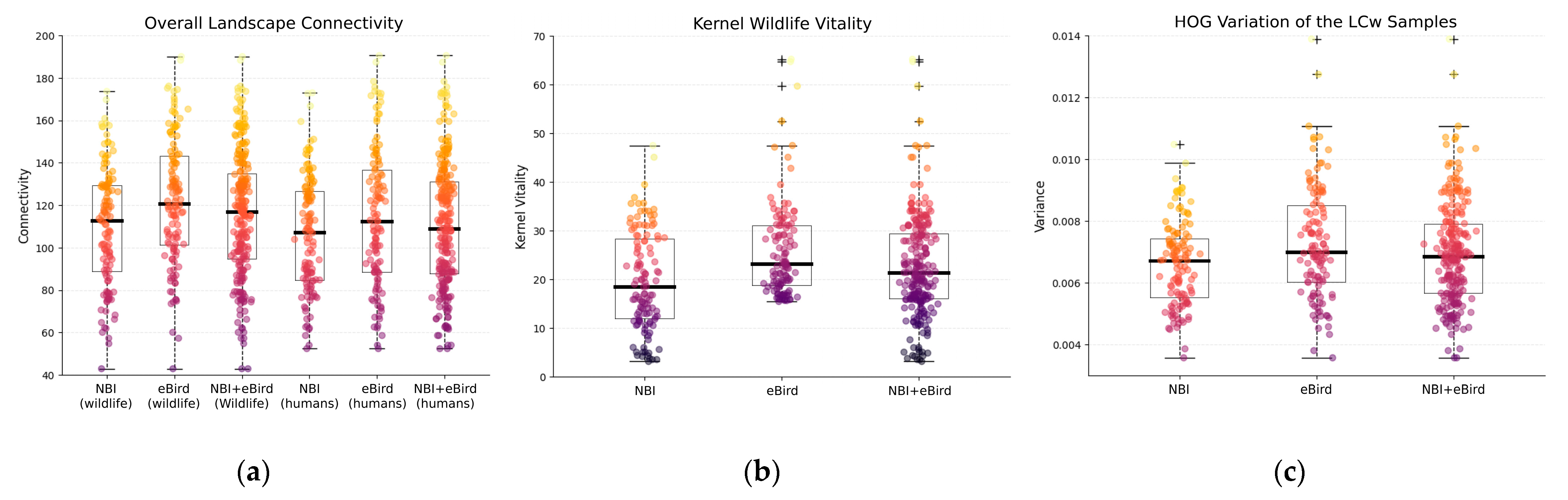
| Overall landscape connectivity (Cm) | ; | The overall landscape connectivity (Cm) can be obtained through connectivity modelling and can be considered as observational data for implicit learning purposes. For one site, the overall landscape connectivity is the mean of the connectivity values of all territorial units (each is represented by one image pixel) within a site. |
| Kernel vitality (Vk) | Weight (V) = 0, if V ∈ Vi 1, if V ∈ Ve and 0 < V < 128 1.5, if V ∈ Ve and 128 ≤ V ≤ 255 Vk = (Σweight(V) for all V in grid)/N; | Scatter plots of eBird data corresponding to each image sample were downloaded for the NBI and eBird datasets, totalling 120 × 2 = 240 images. These scatter plots enable the utilisation of kernel methods and the measurement of observed equivalences within each kernel to interpret their vitality, denoted as Vk. (1) We first divide each scatter plot of the samples into a 200 × 200 grid, where the value of each grid represents a set, V. (2) Second, we classify the values in V as Ve if they are greater than 0 and as Vi if they are equal to 0. (3) Third, we highlight the effect of the scatter plot and increase the weight of the grids in V that are relatively close to the peak value of 255 to 1.5. The weight of the remaining valid grids is 1.0. For each value in Ve, we count it as 1 if it is greater than 0 and less than 192 and count it as 1.5 if it is greater than or equal to 128 and less than or equal to 255. (4) Then, we count each value in Vi as 0. (5) Finally, we sum up all Vi values and all Ve values and then divide the result by 200 × 200. |
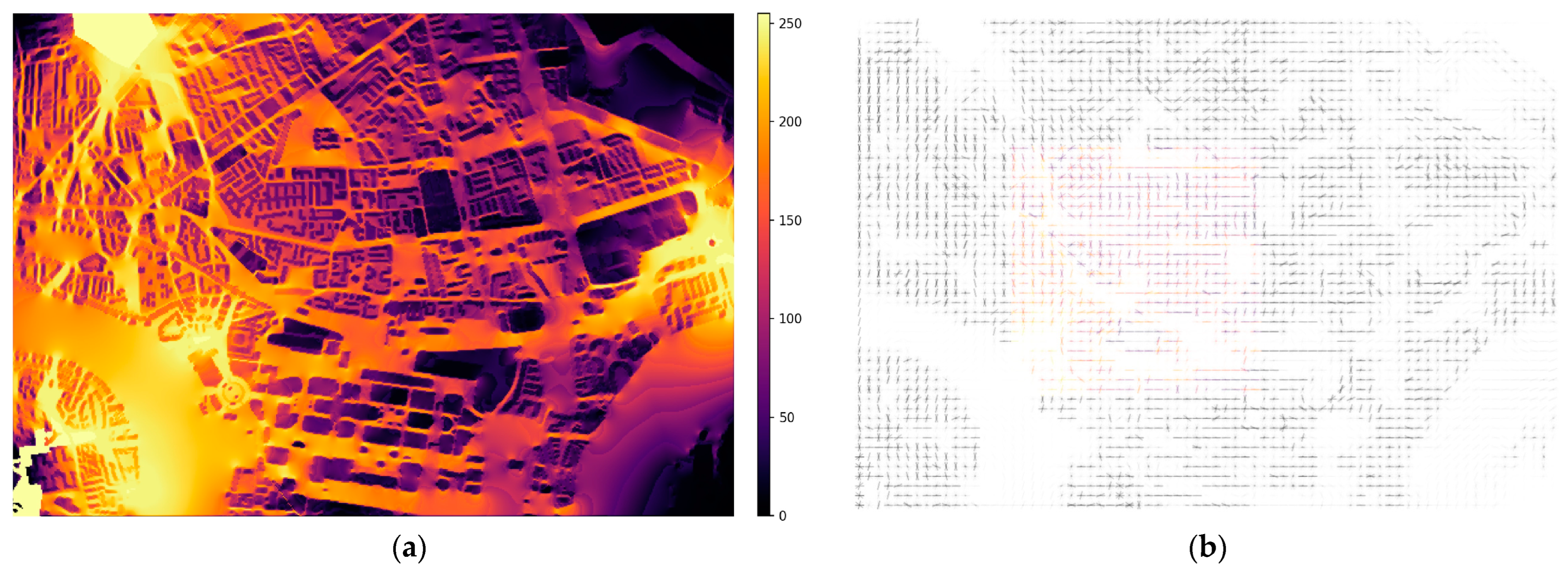
| Histogram of oriented gradients (HOG) gradient computation | Gx = [[−1, 0, 1], [−2, 0, 2], [−1, 0, 1]]; Gy = [[−1, −2, −1], [0, 0, 0], [1, 2, 1]] | (1) Gradient computation: Calculate the gradients of the image using the typical 3 × 3 Sobel filters [62] horizontally (Gx) and vertically (Gy). |
| Histogram of oriented gradients (HOG) gradient magnitude and orientation | M(x, y) = sqrt(Gx (x, y)2 + Gy (x, y)2); θ(x, y) = atan2(Gy (x, y), Gx (x, y)) | (2) Gradient magnitude and orientation: For each pixel (x, y), compute the gradient magnitude (M) and orientation (θ). |
| (3) Divide the image into cells: Split the image into small spatial regions called cells, typically of size 8 × 8 or 16 × 16 pixels. (4) Calculate the histogram of oriented gradients for each cell: For each cell, create a histogram of gradient orientations, typically using 9 orientation bins. Each pixel in the cell contributes to the histogram based on its gradient magnitude and orientation. (5) Normalise histograms of cells within blocks: Group cells into larger regions called blocks (e.g., 2 × 2 cells per block) and normalise the histograms within each block. This step helps in achieving illumination invariance. (6) Concatenate the histograms of all blocks to form the final HOG feature descriptor. In this project, all HOG processes are implemented using the following parameter settings: (16, 16) for kernel size, (2, 2) for block size by cells, orientation as 9, and multichannel as True (taking RGB input). The parameter settings are set according to the “skimage.feature.hog ()” function of scikit-image. The variable settings consider the required minimum size of the information to be observed at the scale of the field and the observability of the HOG image output on the A4 (297 mm × 210 mm) layout. |
References
- Spear, S.F.; Balkenhol, N.; Fortin, M.J.; Mcrae, B.H.; Scribner, K. Use of Resistance Surfaces for Landscape Genetic Studies: Considerations for Parameterization and Analysis. Mol. Ecol. 2010, 19, 3576–3591. [Google Scholar] [CrossRef] [PubMed]
- Aziz, H.A.; Rasidi, M.H. The Role of Green Corridors for Wildlife Conservation in Urban Landscape: A Literature Review. IOP Conf. Ser. Earth Environ. Sci. 2014, 18, 12093. [Google Scholar] [CrossRef]
- Hilty, J.; Worboys, G.L.; Keeley, A.; Woodley, S.; Lausche, B.; Locke, H.; Carr, M.; Pulsford, I.; Pittock, J.; White, J.W. Guidelines for Conserving Connectivity through Ecological Networks and Corridors. Best Pract. Prot. Area Guidel. Ser. 2020, 30, 122. [Google Scholar] [CrossRef]
- Gonzalez-Garcia, A.; Van De Weijer, J.; Bengio, Y. Image-to-Image Translation for Cross-Domain Disentanglement. arXiv 2018, arXiv:1805.09730. [Google Scholar]
- Chang, H.-S.; Liao, C.-H. Exploring an Integrated Method for Measuring the Relative Spatial Equity in Public Facilities in the Context of Urban Parks. Cities 2011, 28, 361–371. [Google Scholar] [CrossRef]
- Ali, M.A.; Kamraju, M. Environmental Justice and Resource Distribution. In Natural Resources and Society: Understanding the Complex Relationship between Humans and the Environment; Springer: Cham, Switaerland, 2023; pp. 159–170. [Google Scholar] [CrossRef]
- Brenner, N.; Schmid, C. Planetary Urbanization. In Infrastructure Space; Ruby, I., Ruby, A., Eds.; Ruby Press: Berlin, Germany, 2017; pp. 37–40. [Google Scholar]
- Zhou, S.; Wang, Y.; Jia, W.; Wang, M.; Wu, Y.; Qiao, R.; Wu, Z. Automatic Responsive-Generation of 3D Urban Morphology Coupled with Local Climate Zones Using Generative Adversarial Network. Build. Environ. 2023, 245, 110855. [Google Scholar] [CrossRef]
- Isola, P.; Zhu, J.-Y.; Zhou, T.; Efros, A.A. Image-to-Image Translation with Conditional Adversarial Networks. In Proceedings of the IEEE Conference on Computer Vision and Pattern Recognition, Honolulu, HA, USA, 21–26 July 2017; pp. 1125–1134. [Google Scholar]
- Huang, W.; Zheng, H. Architectural Drawings Recognition and Generation through Machine Learning. In Proceedings of the ACADIA 2018, Mexico City, Mexico, 18–20 October 2018; pp. 156–165. [Google Scholar]
- Yu, D. Reprogramming Urban Block by Machine Creativity: How to Use Neural Networks as Generative Tools to Design Space. In Proceedings of the eCAADe 2020: Anthropologic, Online, 16–17 September 2020; pp. 1–11. [Google Scholar]
- Zhu, J.-Y.; Park, T.; Isola, P.; Efros, A.A. Unpaired Image-to-Image Translation Using Cycle-Consistent Adversarial Networks. In Proceedings of the IEEE International Conference on Computer Vision, Venice, Italy, 22–29 October 2017; pp. 2223–2232. [Google Scholar]
- Li, Y.; Xu, W. Using Cyclegan to Achieve the Sketch Recognition Process of Sketch-Based Modeling. In Proceedings of the 2021 DigitalFUTURES: The 3rd International Conference on Computational Design and Robotic Fabrication (CDRF 2021), Online, 26 June 2021; pp. 26–34. [Google Scholar]
- Hassab, A.; Abdelmohsen, S.; Abdallah, M. Generative Design Methodology for Double Curved Surfaces Using AI. In Proceedings of the ASCAAD: Architecture in the Age of Distributive Technologies, Cairo, Egypt, 2–4 March 2021; pp. 622–635. [Google Scholar]
- Park, T.; Liu, M.-Y.; Wang, T.-C.; Zhu, J.-Y. GauGAN: Semantic Image Synthesis with Spatially Adaptive Normalization. In Proceedings of the ACM SIGGRAPH 2019 Real-Time Live, Los Angeles, CA, USA, 28 July 2019; p. 1. [Google Scholar]
- Park, T.; Liu, M.-Y.; Wang, T.-C.; Zhu, J.-Y. Semantic Image Synthesis with Spatially-Adaptive Normalization. In Proceedings of the IEEE/CVF Conference on Computer Vision and Pattern Recognition, Long Beach, CA, USA, 15–20 June 2019; pp. 2337–2346. [Google Scholar]
- Salian, I. Stroke of Genius: GauGAN Turns Doodles into Stunning, Photorealistic Landscapes: NVIDIA Research Harnesses Generative Adversarial Networks to Create Highly Realistic Scenes. Available online: https://blogs.nvidia.com/blog/2019/03/18/gaugan-photorealistic-landscapes-nvidia-research/ (accessed on 9 July 2022).
- Chaillou, S. AI + Architecture: Towards a New Approach. Master’s of Architecture, Harvard University, Cambridge, MA, USA, 2019. Available online: https://towardsdatascience.com/architecture-style-ded3a2c3998f (accessed on 16 June 2019).
- Chan, Y.H.E.; Spaeth, A.B. Architectural Visualisation with Conditional Generative Adversarial Networks (cGAN). In Proceedings of the 38th eCAADe Conference, Online, 16–17 September 2020; pp. 299–308. [Google Scholar]
- Alexander, C. Notes on the Synthesis of Form, Paperback ed.; Harvard University Press: Cambridge, MA, USA, 1964; Volume 5, p. 224. [Google Scholar]
- Bhatt, R. Christopher Alexander’s Pattern Language an Alternative Exploration of Space-Making Practices. J. Archit. 2010, 15, 711–729. [Google Scholar] [CrossRef]
- Batty, M. A Theory of Markovian Design Machines. Environ. Plan. B Plan. Des. 1974, 1, 125–146. [Google Scholar] [CrossRef]
- Lystra, M. Drawing Natures: US Highway Location, Representational Techniques and the Rise of Ecological Design. J. Des. Hist. 2017, 30, 157–174. [Google Scholar] [CrossRef]
- Peel, M.C.; Finlayson, B.L.; McMahon, T.A. Updated World Map of the Köppen-Geiger Climate Classification. Hydrol. Earth Syst. Sci. 2007, 11, 1633–1644. [Google Scholar] [CrossRef]
- Gurrutxaga, M.; Lozano, P.; Barrio, G. GIS-Based Approach for Incorporating the Connectivity of Ecological Networks into Regional Planning. J. Nat. Conserv. 2010, 18, 318–326. [Google Scholar] [CrossRef]
- American Museum of Natural History. How to Calculate a Biodiversity Index. Biodiversity Counts Curriculum Collection. 2001. Available online: https://www.amnh.org/learn-teach/curriculum-collections/biodiversity-counts/plant-ecology/how-to-calculate-a-biodiversity-index (accessed on 26 August 2024).
- Delbaere, B. Biodiversity Indicators and Monitoring; European Centre for Nature Conservation: Tilburg, The Netherlands, 2002. [Google Scholar]
- Han, X.; Gill, M.J.; Hamilton, H.; Vergara, S.G.; Young, B.E. Progress on National Biodiversity Indicator Reporting and Prospects for Filling Indicator Gaps in Southeast Asia. Environ. Sustain. Indic. 2020, 5, 100017. [Google Scholar] [CrossRef]
- Jepson, P.; Caldecott, B.; Milligan, H.; Chen, D. A Framework for Protected Area Asset Management. In Stranded Assets Programme; Oxford University: Oxford, UK, 2015. [Google Scholar]
- Auer, T.; Barker, S.; Borgmann, K.; Charnoky, M.; Childs, D.; Curtis, J.; Davies, I.; Downie, I.; Fink, D.; Fredericks, T.; et al. EOD–eBird Observation Dataset; Cornell Lab of Ornithology: Ithaca, NY, USA, 2022. [Google Scholar] [CrossRef]
- Dickson, B.G.; Albano, C.M.; Anantharaman, R.; Beier, P.; Fargione, J.; Graves, T.A.; Gray, M.E.; Hall, K.R.; Lawler, J.J.; Leonard, P.B.; et al. Circuit-Theory Applications to Connectivity Science and Conservation. Conserv. Biol. 2019, 33, 239–249. [Google Scholar] [CrossRef] [PubMed]
- Hall, K.R.; Anantharaman, R.; Landau, V.A.; Clark, M.; Dickson, B.G.; Jones, A.; Platt, J.; Edelman, A.; Shah, V.B. Circuitscape in Julia: Empowering Dynamic Approaches to Connectivity Assessment. Land 2021, 10, 301. [Google Scholar] [CrossRef]
- McRae, B.H.; Dickson, B.G.; Keitt, T.H.; Shah, V.B. Using Circuit Theory to Model Connectivity in Ecology, Evolution, and Conservation. Ecology 2008, 89, 2712–2724. [Google Scholar] [CrossRef]
- Shah, V.B.; McRae, B. Circuitscape: A Tool for Landscape Ecology. In Proceedings of the 7th Python in Science Conference (SciPy 2008), Pasadena, CA, USA, 19–24 August 2008; pp. 62–65. [Google Scholar]
- Belote, R.T.; Barnett, K.; Zeller, K.; Brennan, A.; Gage, J. Examining Local and Regional Ecological Connectivity throughout North America. Landsc. Ecol. 2022, 37, 2977–2990. [Google Scholar] [CrossRef]
- Braaker, S.; Moretti, M.; Boesch, R.; Ghazoul, J.; Obrist, M.K.; Bontadina, F. Assessing Habitat Connectivity for Ground-Dwelling Animals in an Urban Environment. Ecol. Appl. 2014, 24, 1583–1595. [Google Scholar] [CrossRef] [PubMed]
- Carroll, K.A.; Hansen, A.J.; Inman, R.M.; Lawrence, R.L.; Hoegh, A.B. Testing Landscape Resistance Layers and Modeling Connectivity for Wolverines in the Western United States. Glob. Ecol. Conserv. 2020, 23, e01125. [Google Scholar] [CrossRef]
- Hetherington, D.; Gorman, M. Using Prey Densities to Estimate the Potential Size of Reintroduced Populations of Eurasian Lynx. Biol. Conserv. 2007, 137, 37–44. [Google Scholar] [CrossRef]
- Hetherington, D.A.; Miller, D.R.; Macleod, C.D.; Gorman, M.L. A Potential Habitat Network for the Eurasian Lynx in Scotland. Mamm. Rev. 2008, 38, 285–303. [Google Scholar] [CrossRef]
- Özcan, A.U.; Erzin, P.E. Assessment of Gis-Assisted Movement Patches Using Lcp for Local Species: North Central Anatolia Region, Turkey. Cerne 2020, 26, 130–139. [Google Scholar] [CrossRef]
- Batha, V.L.; Otawa, T. Incorporating Wildlife Conservation within Local Land Use Planning and Zoning: Ability of Circuitscape to Model Conservation Corridors. In Proceedings of the Fábos Conference on Landscape and Greenway Planning, Amherst, MA, USA, 12–13 April 2013; Volume 4, p. 15. [Google Scholar] [CrossRef]
- Herrera, J.M.; Alagador, D.; Salgueiro, P.; Mira, A. A Distribution-Oriented Approach to Support Landscape Connectivity for Ecologically Distinct Bird Species. PLoS ONE 2018, 13, e0194848. [Google Scholar] [CrossRef] [PubMed]
- Grafius, D.R.; Corstanje, R.; Siriwardena, G.M.; Plummer, K.E.; Harris, J.A. A Bird’s Eye View: Using Circuit Theory to Study Urban Landscape Connectivity for Birds. Landsc. Ecol. 2017, 32, 1771–1787. [Google Scholar] [CrossRef] [PubMed]
- Howey, M.C.L. Multiple Pathways across Past Landscapes: Circuit Theory as a Complementary Geospatial Method to Least Cost Path for Modeling Past Movement. J. Archaeol. Sci. 2011, 38, 2523. [Google Scholar] [CrossRef]
- Barbosa, H.; Barthelemy, M.; Ghoshal, G.; James, C.R.; Lenormand, M.; Louail, T.; Menezes, R.; Ramasco, J.J.; Simini, F.; Tomasini, M. Human Mobility: Models and Applications. Phys. Rep. 2018, 734, 1–74. [Google Scholar] [CrossRef]
- Wang, Y.; Qiu, W.; Jiang, Q.; Li, W.; Ji, T.; Dong, L. Drivers or Pedestrians, Whose Dynamic Perceptions Are More Effective to Explain Street Vitality? A case study in Guangzhou. Remote Sens. 2023, 15, 568. [Google Scholar] [CrossRef]
- McRae, B.; Shah, V.; Mohapatra, T.; Ranjan, A. Circuitscape (Version Circuitscape 4.0). 2008. Available online: https://circuitscape.org/downloads/circuitscape_4_0.pdf (accessed on 14 January 2023).
- Almenar, J.B.; Bolowich, A.; Elliot, T.; Geneletti, D.; Sonnemann, G.; Rugani, B. Assessing Habitat Loss, Fragmentation and Ecological Connectivity in Luxembourg to Support Spatial Planning. Landsc. Urban Plan. 2019, 189, 335–351. [Google Scholar] [CrossRef]
- Carroll, C. Linking Connectivity to Viability: Insights from Spatially Explicit Population Models of Large Carnivores. In Connectivity Conservation, 1st ed.; Crooks, K.R., Sanjayan, M., Eds.; Cambridge University Press: Cambridge, UK, 2006; pp. 369–389. [Google Scholar]
- Crooks, K.R.; Sanjayan, M. (Eds.) Connectivity Conservation, 1st ed.; Cambridge University Press: Cambridge, UK, 2006. [Google Scholar]
- Ferreras, P. Landscape Structure and Asymmetrical Inter-Patch Connectivity in a Metapopulation of the Endangered Iberian lynx. Biol. Conserv. 2001, 100, 125–136. [Google Scholar] [CrossRef]
- Schneider, C.; Fry, G. Estimating the Consequences of Land-Use Changes on Butterfly Diversity in a Marginal Agricultural Landscape in Sweden. J. Nat. Conserv. 2005, 13, 247–256. [Google Scholar] [CrossRef]
- Zimmermann, F.; Breitenmoser, U. Potential Distribution and Population Size of the Eurasian Lynx Lynx Lynx in the Jura Mountains and Possible Corridors to Adjacent Ranges. Wildl. Biol. 2007, 13, 406–416. [Google Scholar] [CrossRef]
- Dalal, N.; Triggs, B. Histograms of Oriented Gradients for Human Detection. In Proceedings of the 2005 IEEE Computer Society Conference on Computer Vision and Pattern Recognition (CVPR’05), San Diego, CA, USA, 20–25 June 2005; pp. 886–893. [Google Scholar]
- Rugg, L.H. Ecology and Culture in Scandinavia. Available online: https://olli.berkeley.edu/sites/default/files/course/documents/ecosyllolli.pdf (accessed on 8 December 2019).
- Magnussen, K.; Dombu, S.V. Nordic Ecosystem Services. Available online: https://www.menon.no/wp-content/uploads/Nordic-Ecosystem-Services-MERE.pdf (accessed on 27 July 2022).
- del Campo, M.; Manninger, S.; Carlson, A. Imaginary Plans. In Proceedings of the ACADIA 2019: Ubiquity and Autonomy, Austin, TX, USA, 21–26 October 2019; pp. 412–418. [Google Scholar]
- Mirza, M.; Osindero, S. Conditional Generative Adversarial nets. arXiv 2014, arXiv:1411.1784. [Google Scholar]
- Cherry, L.; Haralambidou, P.; Migayrou, F.; Porter, A. (Eds.) The Bartlett School of Architecture, Ucl: B-Pro Show 2020, Paperback ed.; The Bartlett School of Architecture, UCL: London, UK, 2020; Available online: https://bproautumn2020.bartlettarchucl.com/rc18/glitch-arch (accessed on 2 October 2020).
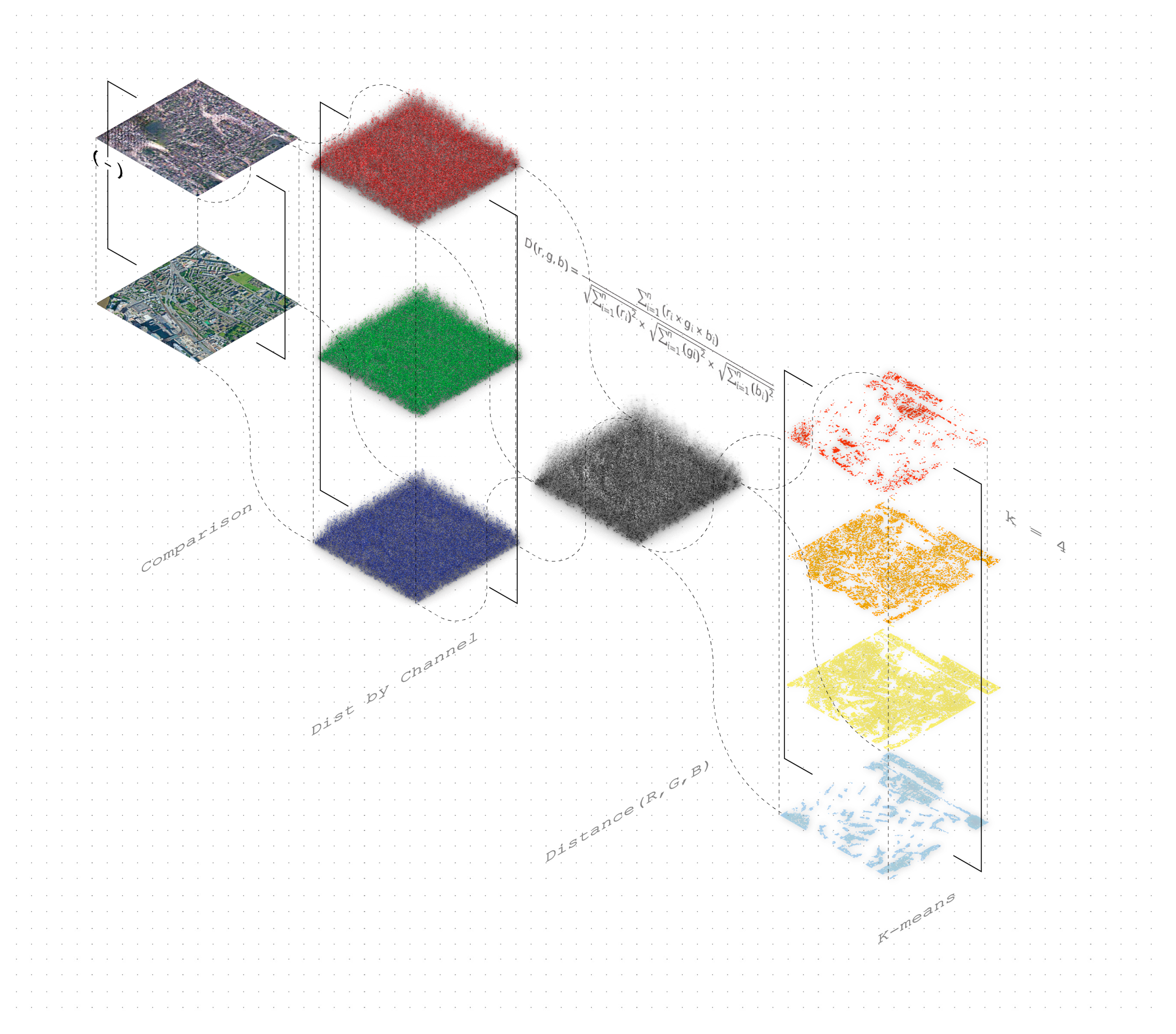
- Neto, S.L.M.; Von Wangenheim, A.; Pereira, E.B.; Comunello, E. The Use of Euclidean Geometric Distance on RGB Color Space for the Classification of Sky and Cloud Patterns. J. Atmos. Ocean. Technol. 2010, 27, 1504–1517. [Google Scholar] [CrossRef]
- Syakur, M.A.; Khotimah, B.K.; Rochman, E.; Satoto, B.D. Integration K-Means Clustering Method and Elbow Method for Identification of the Best Customer Profile Cluster. IOP Conf. Ser. Mater. Sci. Eng. 2018, 336, 012017. [Google Scholar] [CrossRef]
- Szeliski, R. Computer Vision: Algorithms and Applications; Springer Science & Business Media: Berlin/Heidelberg, Germany, 2010. [Google Scholar]


| Symbol | Implication | |
|---|---|---|
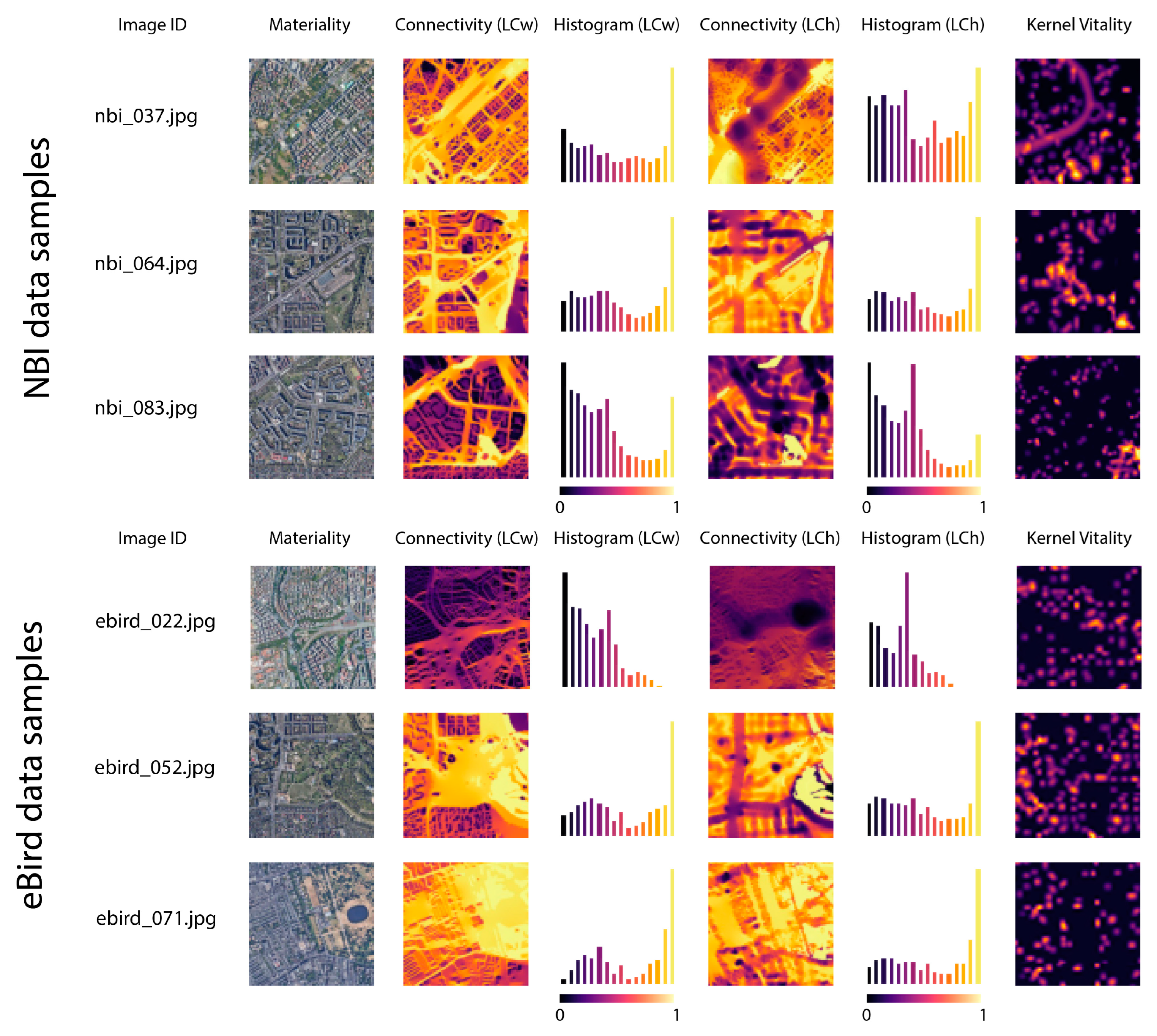
| LCh | Human landscape connectivity | |
| LCh’ | Human landscape connectivity of the site | |
| LCw | Wildlife landscape connectivity | |
| LCw’ | Wildlife landscape connectivity of the site | |
| Cm | Overall connectivity metric | |
| Vk | Kernel connectivity vitality | weight(V) = 0, if V ∈ Vi 1, if V ∈ Ve and 0 < V < 128 1.5, if V ∈ Ve and 128 ≤ V ≤ 255 Vk = (Σweight(V) for all V in grid)/N |
| Factor (Wildlife) | Sub-Factor | Resistance Value (Ours) | Resistance Value [25] | Resistance Value [40] | Resistance Value [41] | |
|---|---|---|---|---|---|---|
| Local scale | Buildings | With buildings blocking | 1000 | / | / | 500 (maximum 500) |
| Without buildings blocking | 100 | / | / | 100 (minimum 100) | ||
| City scale | Land use | Urban | 1000 | 1000 | 1000 | 500 |
| Industrial | 1000 | / | 1000 | 500 | ||
| Water | 100 | 100 | 1000 | 100 | ||
| Quarries | 100 | 90 | 1000 | 250 | ||
| Crops | 60 | 60 | 60 | 400–500 | ||
| Grassland | 40 | 30–40 | 40 | 100–500 | ||
| Forest | 10 | 1–20 | 10 | 100 | ||
| Roads | <1000 vehicles/day | 80 | 80 | 80 | / | |
| 1000–5000 vehicles/day | 100 | 100 | 100 | / | ||
| 5000–10,000 vehicles/day | 300 | 300 | 300 | / | ||
| 10,000–20,000 vehicles/day | 700 | 700 | 700 | / | ||
| >20,000 vehicles/day | 800 | 800 | 800 | / | ||
| Distance to road: 0.4 km | / | / | / | 250 | ||
| Distance to road: 0.8 km | / | / | / | 500 | ||
| Rivers | Large river (>30 m width) | 120 | 120 | 120 | / | |
| Medium river (<30 m width) | 40 | 40 | 40 | / | ||
| Distance to stream: 0.8 km–3.21 km | / | / | / | 100–300 | ||
| Distance to stream: 3.21 km–9.65 km | / | / | / | 300–500 | ||
| Factor (human) | Sub-factor | Resistance value (ours) | ||||
| Local scale | Buildings | With buildings blocking | 1000 | |||
| Without buildings blocking | 100 | |||||
| City scale | Kernel density of POI aggregation (Search radius) | 0–25 m | 1000 | |||
| 25–50 m | 500 | |||||
| 50–100 m | 200 | |||||
| 100–200 m | 100 | |||||
| 200–300 m | 60 | |||||
| 300–800 m | 40 | |||||
| >800 m | 10 | |||||
| Roads | <1000 vehicles/day | 80 | ||||
| 1000–5000 vehicles/day | 100 | |||||
| 5000–10,000 vehicles/day | 300 | |||||
| 10,000–20,000 vehicles/day | 700 | |||||
| >20,000 vehicles/day | 800 | |||||
| Rivers | Large river (>30 m width) | 1000 | ||||
| Medium river (<30 m width) | 1000 | |||||
| Analytical Metrics | NBI Dataset | eBird Dataset | ||||
|---|---|---|---|---|---|---|
| Mean | Maximum | Minimum | Mean | Maximum | Minimum | |
| Overall landscape connectivity for wildlife (LCw) | 109.951 | 173.689 | 42.839 | 122.215 | 190.031 | 42.839 |
| Overall landscape connectivity for human (LCh) | 106.373 | 173.587 | 55.464 | 114.699 | 190.013 | 54.574 |
| kernel vitality (Vk) | 19.741 | 47.520 | 3.150 | 25.949 | 65.240 | 15.460 |
| Histogram of oriented gradients (HOG) | 0.006 | 0.010 | 0.003 | 0.007 | 0.013 | 0.003 |
| Hyperparameter | Settings |
|---|---|
| Deep learning platform | TensorFlow 2.9 and Keras |
| Buffer size | 400 |
| Batch size | 1 |
| Image I/O shape | Width, depth, channel = (256, 256, 3) |
| Data augmentation | Resizing, random rotation, normalisation |
| Generator optimizer | Adam |
| Discriminator optimizer | Adam |
| Lambda | 100 |
| Learning rate of generator | 0.0002 |
| Learning rate of discriminator | 0.0002 |
| Epoch | 1000 |
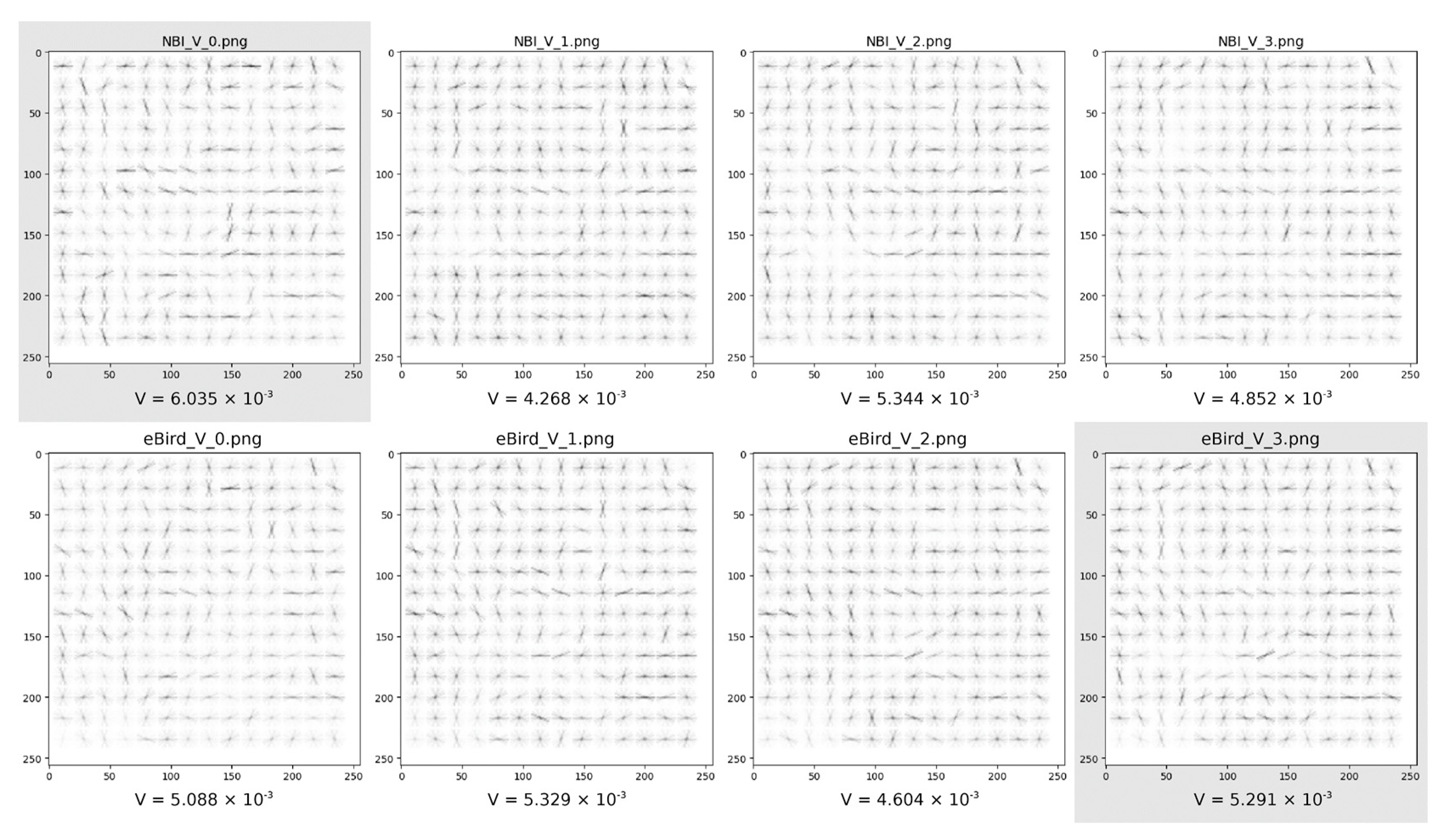
| LCW’ Candidate ID | Predicted HOG Variance | Measured HOG Variance | Distance (Absolute) |
|---|---|---|---|
| NBI_LCw’_0.png | 0.0059754900 | 0.004851629 | 0.0000594910 |
| NBI _LCw’_1.png | 0.0057605545 | 0.005343917 | 0.0014930026 |
| NBI _LCw’_2.png | 0.0059387909 | 0.004267552 | 0.0005948741 |
| NBI _LCw’_3.png | 0.0058972843 | 0.006034981 | 0.0010456553 |
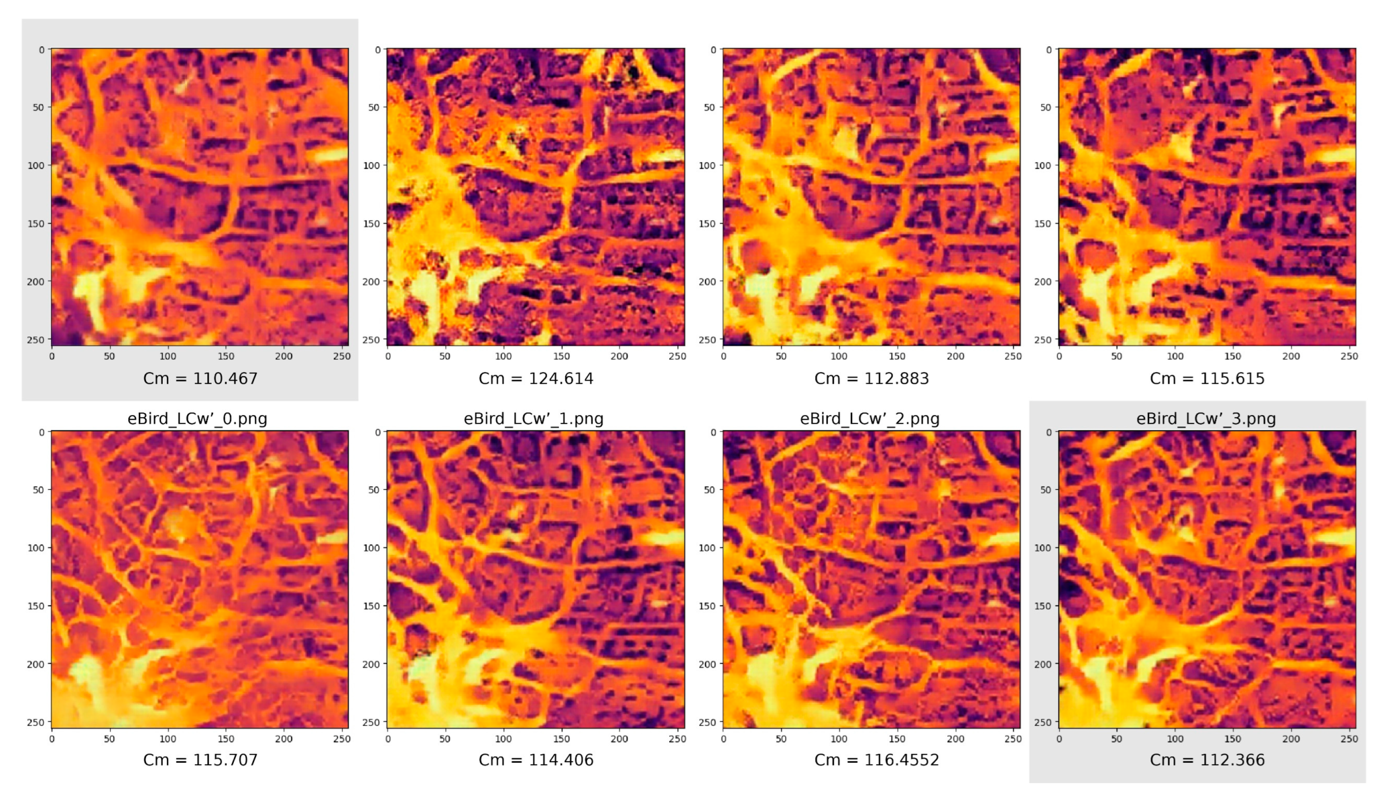
| eBird_LCw’_0.png | 0.0058958727 | 0.0050879717 | 0.0008079010 |
| eBird_LCw’_1.png | 0.0059156528 | 0.0053285174 | 0.0005871354 |
| eBird_LCw’_2.png | 0.0058830485 | 0.0046036155 | 0.0012794330 |
| eBird_LCw’_3.png | 0.0057947158 | 0.0052909655 | 0.0005037503 |
Disclaimer/Publisher’s Note: The statements, opinions and data contained in all publications are solely those of the individual author(s) and contributor(s) and not of MDPI and/or the editor(s). MDPI and/or the editor(s) disclaim responsibility for any injury to people or property resulting from any ideas, methods, instructions or products referred to in the content. |
© 2024 by the authors. Licensee MDPI, Basel, Switzerland. This article is an open access article distributed under the terms and conditions of the Creative Commons Attribution (CC BY) license (https://creativecommons.org/licenses/by/4.0/).
Share and Cite
Huang, S.-Y.; Wang, Y.; Llabres-Valls, E.; Jiang, M.; Chen, F. Meta-Connectivity in Urban Morphology: A Deep Generative Approach for Integrating Human–Wildlife Landscape Connectivity in Urban Design. Land 2024, 13, 1397. https://doi.org/10.3390/land13091397
Huang S-Y, Wang Y, Llabres-Valls E, Jiang M, Chen F. Meta-Connectivity in Urban Morphology: A Deep Generative Approach for Integrating Human–Wildlife Landscape Connectivity in Urban Design. Land. 2024; 13(9):1397. https://doi.org/10.3390/land13091397
Chicago/Turabian StyleHuang, Sheng-Yang, Yuankai Wang, Enriqueta Llabres-Valls, Mochen Jiang, and Fei Chen. 2024. "Meta-Connectivity in Urban Morphology: A Deep Generative Approach for Integrating Human–Wildlife Landscape Connectivity in Urban Design" Land 13, no. 9: 1397. https://doi.org/10.3390/land13091397