

Spatio-Temporal Diversification of per Capita Carbon Emissions in China: 2000–2020

Abstract
:1. Introduction
2. Materials and Methods
2.1. Study Area
2.2. Data Sources
2.3. Per Capita Carbon Emissions
2.4. Markov Chain
2.5. Kernel Density Analysis
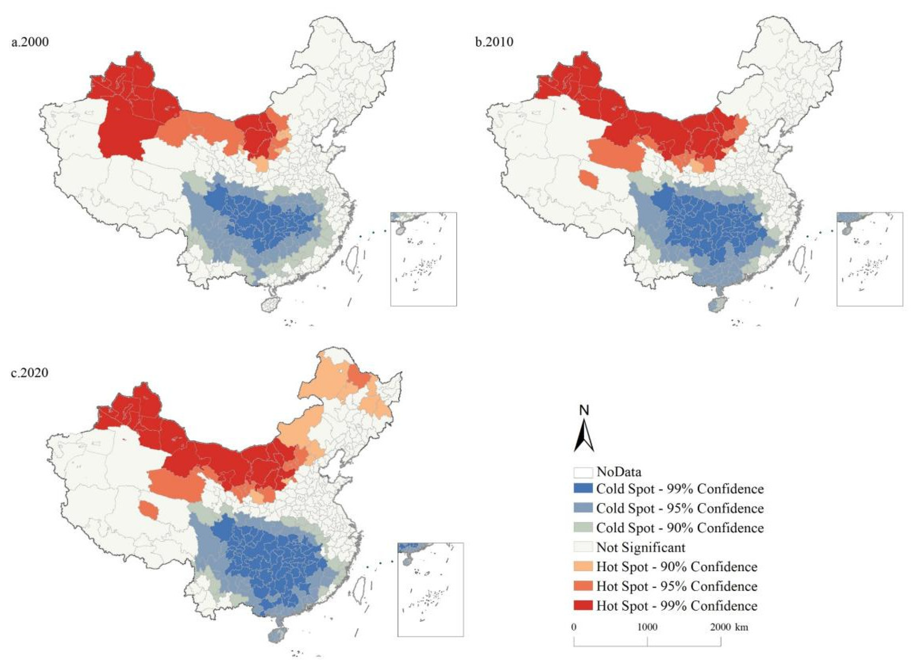
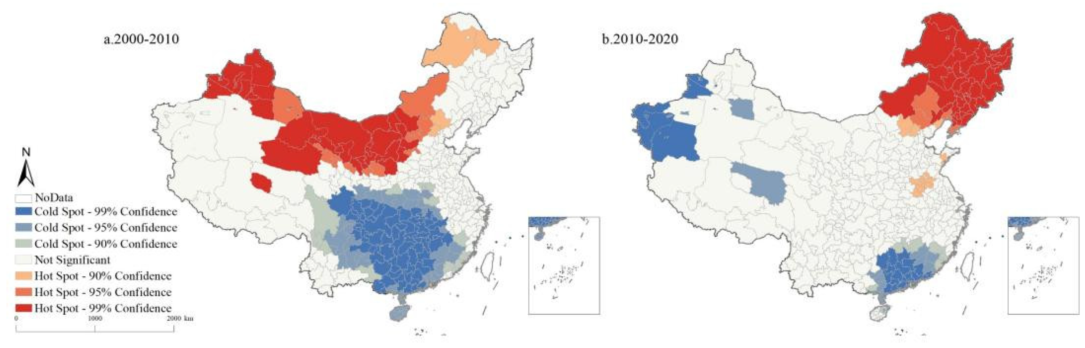
2.6. Hotspots Analysis
2.7. Spatial Regression
3. Results
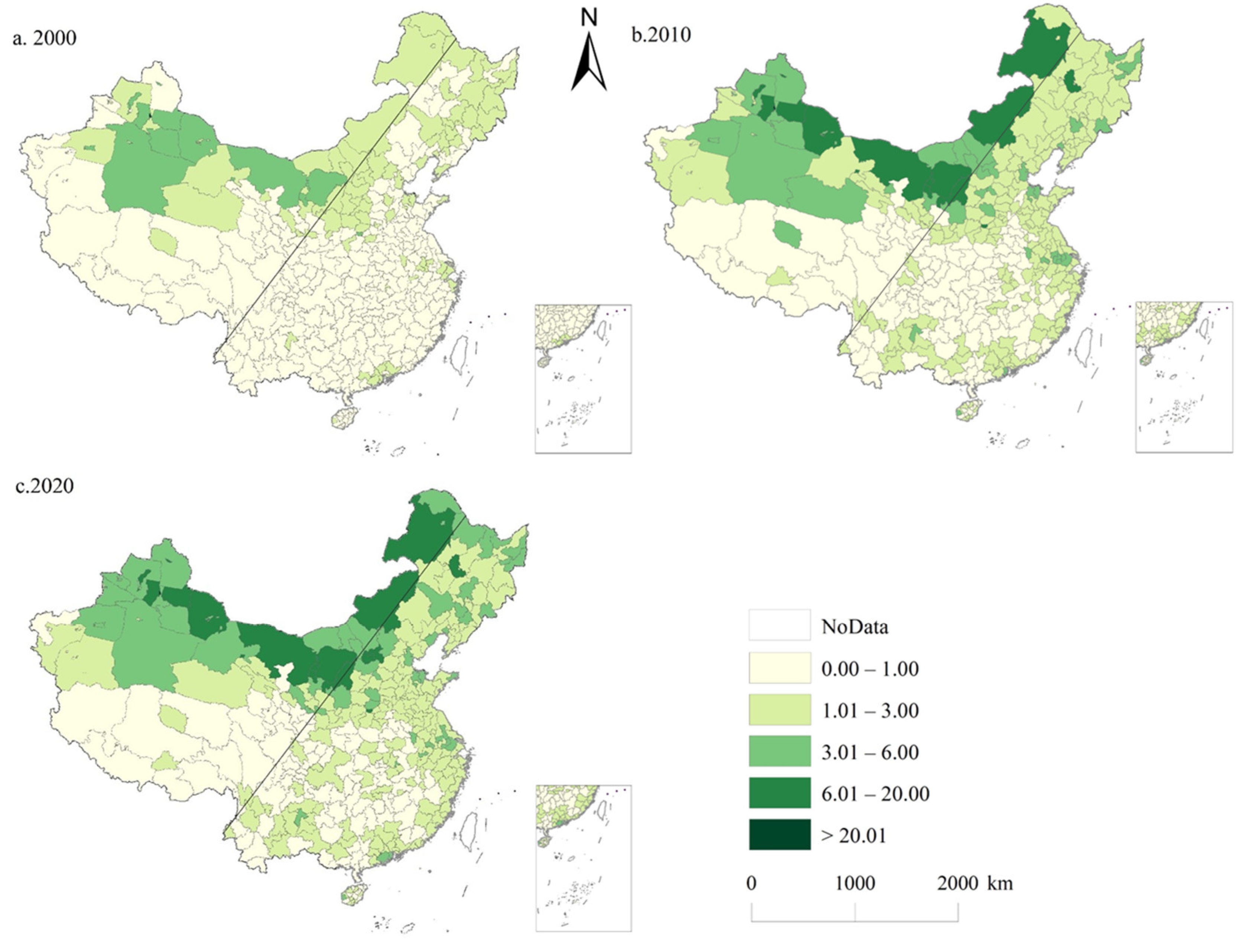
3.1. PCEs in China
3.2. Spatiotemporal Dynamics of PCEs
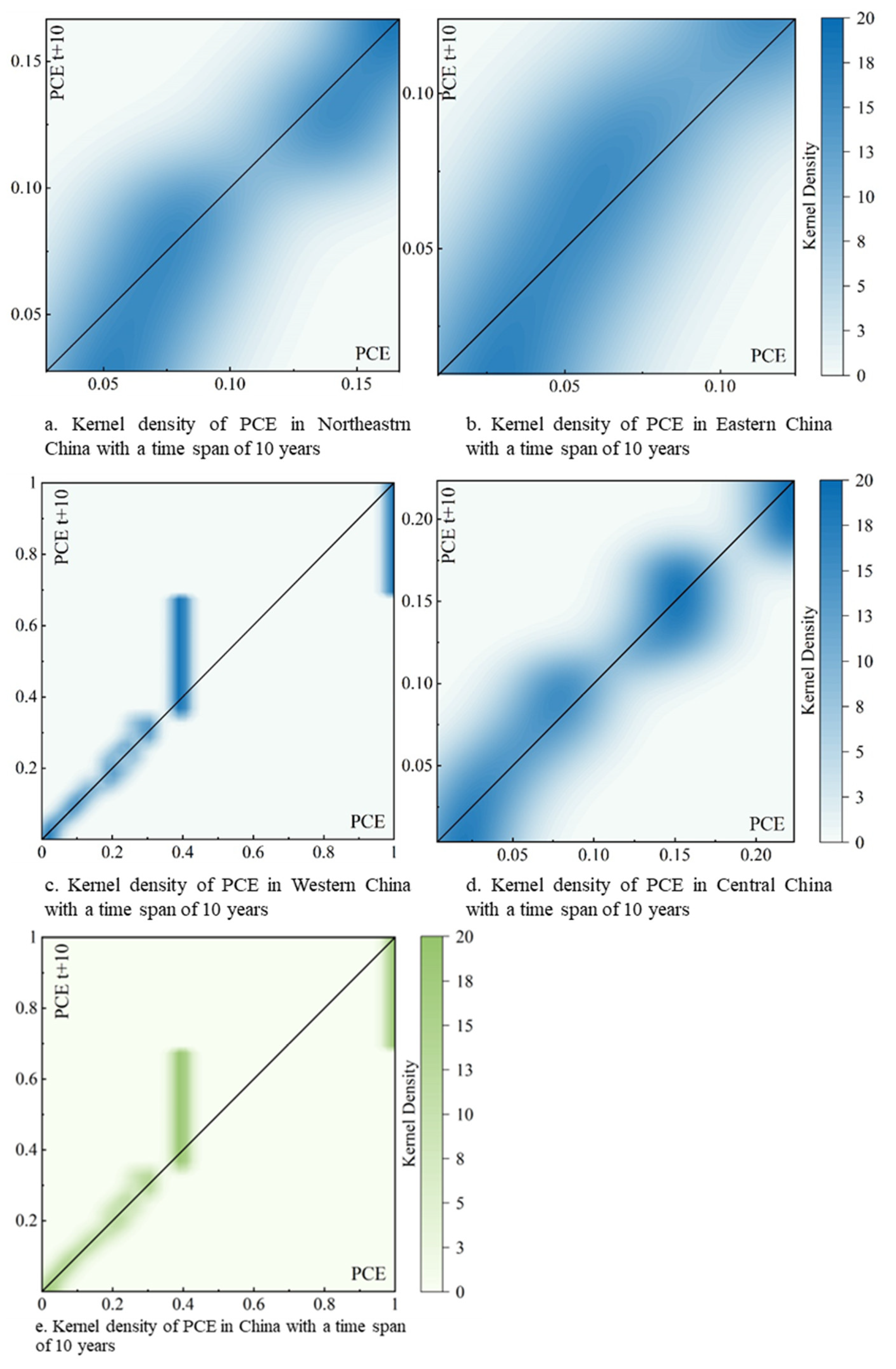
3.3. Kernel Density
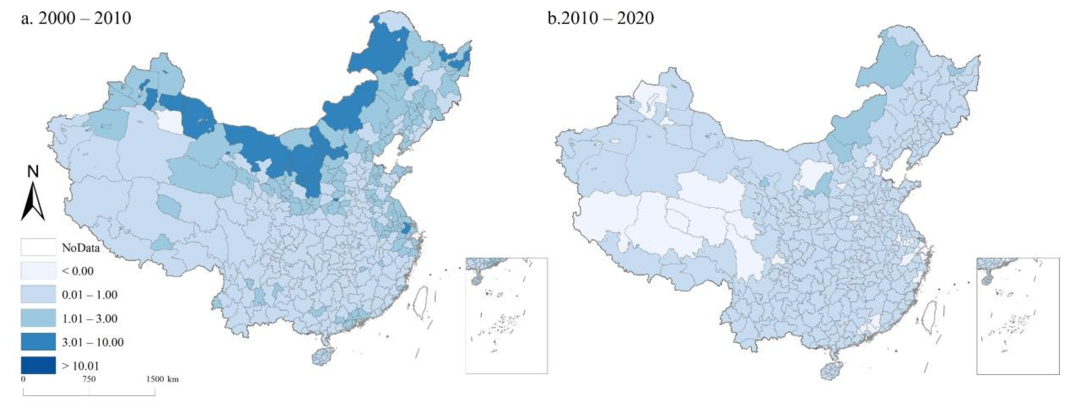
3.4. Change in PCEs in China
3.5. Driving Mechanism of Low-Carbon Transition
4. Discussion
4.1. Interpretation of Findings
4.2. Driving Mechanisms of Low-Carbon Transition
4.3. Policy Implications of Low-Carbon Transition
4.3.1. Promoting the Low-Carbon Transition
4.3.2. Focusing on the Spatial Agglomeration Effects of PCE
4.3.3. Coordinating Economic Growth and CEs
4.3.4. Formulating Differential Strategy
5. Conclusions
Author Contributions
Funding
Data Availability Statement
Conflicts of Interest
References
- Bakhtyar, B.; Ibrahim, Y.; Alghoul, M.A.; Aziz, N.; Fudholi, A.; Sopian, K. Estimating the CO2 abatement cost: Substitute price of avoiding CO2 emission (SPAE) by renewable energy’s feed in tariff in selected countries. Renew. Sustain. Energy Rev. 2014, 35, 205–210. [Google Scholar] [CrossRef]
- Gökmenoğlu, K.; Taspinar, N. The relationship between CO2 emissions, energy consumption, economic growth and FDI: The case of Turkey. J. Int. Trade. Econ. Dev. 2016, 25, 706–723. [Google Scholar] [CrossRef]
- Allen, M.R.; Frame, D.J.; Huntingford, C.; Jones, C.D.; Meinshausen, N. Warming caused by cumulative carbon emissions towards the trillionth tonne. Nature 2009, 458, 1163–1166. [Google Scholar] [CrossRef] [PubMed]
- Höhne, N.; den Elzen, M.; Rogelj, J.; Metz, B.; Fransen, T.; Kuramochi, T.; Olhoff, A.; Alcamo, J.; Winkler, H.; Fu, S.; et al. Emissions: World has four times the work or one-third of the time. Nature 2020, 579, 25–28. [Google Scholar] [CrossRef] [PubMed]
- Meinshausen, M.; Meinshausen, N.; Hare, W.; Raper, S.C.; Frieler, K.; Knutti, R.; Frame, D.J.; Allen, M.R. Greenhouse-gas emission targets for limiting global warming to 2 C′. Nature 2009, 458, 1158–1162. [Google Scholar] [CrossRef]
- Climate Watch. Historical GHG Emissions. 2024. Available online: https://www.climatewatchdata.org/ghg-emissions (accessed on 26 August 2024).
- Söderholm, P.; Hildingsson, R.; Johansson, B.; Khan, J.; Wilhelmsson, F. Governing the transition to low-carbon futures: A critical survey of energy scenarios for 2050. Futures 2011, 43, 1105–1116. [Google Scholar] [CrossRef]
- Wang, S.B.; Liu, H.M.; Pu, H.X.; Yang, H. Spatial disparity and hierarchical cluster analysis of final energy consumption in China. Energy 2020, 197, 117195. [Google Scholar] [CrossRef]
- Hickel, J. Quantifying national responsibility for climate break down:an equality-based attribution approach for carbon dioxide emissions in excess of the planetary boundary. Lancet Planet. Health 2020, 4, e399–e404. [Google Scholar] [CrossRef]
- Matthews, H.D. Quantifying historical carbon and climate debts among nations. Nat. Clim. Chang. 2016, 6, 60–64. [Google Scholar] [CrossRef]
- Adriana, D.B.; Michela, G.; Nicolò, S.; Baccelli, O.; Croci, E.; Molteni, T. Impact of circular measures to reduce urban CO2 emissions: An analysis of four case studies through a production- and consumption-based emission accounting method. J. Clean. Prod. 2022, 380, 134932. [Google Scholar]
- Ali, U.; Guo, Q.B.; Zhanar, N.; Nurgazina, Z.; Sharif, A.; Kartal, M.T.; Depren, S.K.; Khan, A. Heterogeneous impact of industrialization, foreign direct investments, and technological innovation on carbon emissions intensity: Evidence from Kingdom of Saudi Arabia. Appl. Energy 2023, 336, 120804. [Google Scholar] [CrossRef]
- Wang, Z.; Zeng, Y.; Wang, X.; Gu, T.; Chen, W. Impact of urban expansion on carbon emissions in the urban agglomerations of Yellow River Basin, China. Land 2024, 13, 651. [Google Scholar] [CrossRef]
- Shi, Y.; Han, B.; Han, L.; Wei, Z. Uncovering the national and regional household carbon emissions in China using temporal and spatial decomposition analysis models. J. Clean. Prod. 2019, 232, 966–979. [Google Scholar] [CrossRef]
- Huo, T.; Xu, L.; Feng, W.; Cai, W.; Liu, B. Dynamic scenario simulations of carbon emission peak in China’s city-scaleurban residential building sector through 2050. Sci. Total Environ. 2021, 159, 112612. [Google Scholar]
- Wang, S.J.; Huang, Y.Y. Spatial spillover effect and driving forces of carbon emission intensity at city level in China. Acta Geogr. Sin. 2019, 74, 1131–1148. (In Chinese) [Google Scholar] [CrossRef]
- Li, S.L.; Wang, Z.Z. The effects of agricultural technology progress on agricultural carbon emission and carbon sink in China. Agriculture 2023, 13, 793. [Google Scholar] [CrossRef]
- Chen, C.H.; Luo, Y.Q.; Zhou, H.; Huang, J.B. Understanding the driving factors and finding the pathway to mitigating carbon emissions in China’s Yangtze River Delta region. Energy 2023, 278, 127897. [Google Scholar] [CrossRef]
- Wang, S.; Xie, Z.; Wu, R.; Feng, K. How does urbanization affect the carbon intensity of human well-being? A global assessment. Appl. Energy 2022, 312, 118798. [Google Scholar] [CrossRef]
- Zhou, Y.Q.; Zou, S.; Duan, W.L.; Chen, Y.N.; Takara, K.R.; Di, Y.F. Analysis of energy carbon emissions from agroecosystems in Tarim River Basin, China: A pathway to achieve carbon neutrality. Appl. Energy 2022, 325, 119842. [Google Scholar] [CrossRef]
- Huang, Y.M.; Zhang, Y.N. Digitalization, positioning in global value chain and carbon emissions embodied in exports: Evidence from global manufacturing production-based emissions. Ecol. Econ. 2023, 205, 107674. [Google Scholar] [CrossRef]
- Wang, S.J.; Fang, C.L.; Wang, Y. Spatiotemporal variations of energy-related CO2 emissions in China and its influencing factors: An empirical analysis based on provincial panel data. Renew. Sustain. Energy Rev. 2016, 55, 505–515. [Google Scholar] [CrossRef]
- Ehigiamusoe, K.U.; Shahbaz, M.; Vo, X.V. How Does Globalization Influence the Impact of Tourism on Carbon Emissions and Ecological Footprint? Evidence from African Countries. J. Travel. Res. 2023, 62, 1010–1032. [Google Scholar] [CrossRef]
- Jan, S.; Liu, Y.; Stefan, S. Carbon emissions from European land transportation: A comprehensive analysis. Transp. Res. Part D Transp. Environ. 2023, 121, 103851. [Google Scholar]
- Zhang, C.Y.; Zhang, H.T.; Chen, M.N.; Fang, R.Y.; Yao, Y.; Zhang, Q.P.; Wang, Q. Spatial-temporal characteristics of carbon emissions from land use change in Yellow River Delta region. China Ecol. Indic. 2022, 136, 108623. [Google Scholar] [CrossRef]
- Dogan, E.; Turkekul, B. CO2 emissions, real output, energy consumption, trade, urbanization and financial development: Testing the EKC hypothesis for the USA. Environ. Sci. Pollut. Res. 2016, 23, 1203–1213. [Google Scholar] [CrossRef]
- Erdogan, S. Dynamic nexus between technological innovation and building sector carbon emissions in the BRICS Countries. J. Environ. Manag. 2021, 293, 112780. [Google Scholar] [CrossRef] [PubMed]
- Chen, X.L.; Di, Q.B.; Jia, W.H.; Hou, Z.W. Spatial correlation network of pollution and carbon emission reductions coupled with high-quality economic development in three Chinese urban agglomerations. Sustain. Cities Soc. 2023, 94, 104552. [Google Scholar] [CrossRef]
- Wu, H.; Yang, Y.; Li, W. Analysis of spatiotemporal evolution characteristics and peak forecast of provincial carbon emissions under the dual carbon goal: Considering nine provinces in the Yellow River basin of China as an example. Atmos. Pollut. Res. 2023, 14, 101828. [Google Scholar] [CrossRef]
- Fan, J.J.; Wang, J.L.; Qiu, J.X.; Li, N. Stage effects of energy consumption and carbon emissions in the process of urbanization: Evidence from 30 provinces in China. Energy 2023, 276, 127655. [Google Scholar] [CrossRef]
- Liu, Q.F.; Song, J.P.; Dai, T.Q.; Shi, A.; Xu, J.H.; Wang, E.R. Spatio-temporal dynamic evolution of carbon emission intensity and the effectiveness of carbon emission reduction at county level based on nighttime light data. J. Clean. Prod. 2022, 362, 132301. [Google Scholar] [CrossRef]
- Liu, H.; Lei, J. The impacts of urbanization on Chinese households’ energy consumption: An energy input-output analysis. J. Renew. Sustain. Energy 2018, 10, 015903. [Google Scholar] [CrossRef]
- Wang, S.J.; Liu, X.P. China’s city-level energy-related CO2 emissions: Spatiotemporal patterns and driving forces. Appl. Energy 2017, 200, 204–214. [Google Scholar] [CrossRef]
- Zhang, Y.J.; Hao, J.F.; Song, J. The CO2 emission efficiency, reduction potential and spatial clustering in China’s industry: Evidence from the regional level. Appl. Energy 2016, 174, 213–223. [Google Scholar] [CrossRef]
- Chen, W.X.; Chi, G.Q. Ecosystem services trade-offs and synergies in China, 2000–2015. Int. J. Environ. Sci. Technol. 2022, 20, 3221–3236. [Google Scholar] [CrossRef]
- Chancel, L. Global carbon inequality over 1990–2019. Nat. Sustain. 2022, 5, 931–938. [Google Scholar] [CrossRef]
- Ma, T.; Liu, Y.S.; Yang, M. Spatial-temporal heterogeneity for commercial building carbon emissions in China: Based the dagum gini coefficient. Sustainability 2022, 14, 5243. [Google Scholar] [CrossRef]
- Tao, M.M.; Sheng, M.S.; Wen, L. How does financial development influence carbon emission intensity in the OECD countries: Some insights from the information and communication technology perspective. J. Environ. Manag. 2023, 335, 117553. [Google Scholar] [CrossRef]
- Jebli, M.B.; Kahia, M. The interdependence between CO2 emissions, economic growth, renewable and non-renewable energies, and service development: Evidence from 65 countries. Clim. Chang. 2020, 162, 193–212. [Google Scholar] [CrossRef]
- Akram, R.; Umar, M.; Gan, X.L.; Chen, F. Dynamic linkages between energy efficiency, renewable energy along with economic growth and carbon emission. A case of MINT countries an asymmetric analysis. Energy Rep. 2022, 8, 2119–2130. [Google Scholar] [CrossRef]
- Nasir, M.A.; Huynh, T.L.D.; Tram, H.T.X. Role of financial development, economic growth & foreign direct investment in driving climate change: A case of emerging ASEAN. J. Environ. Manag. 2019, 242, 131–141. [Google Scholar]
- Chen, W.X.; Wang, G.Z.; Xu, N.; Ji, M.; Zeng, J. Promoting or inhibiting? New-type urbanization and urban carbon emissions efficiency in China. Cities 2023, 140, 104429. [Google Scholar] [CrossRef]
- Tang, Z.P.; Wang, L.H.; Wu, W. The impact of high-speed rail on urban carbon emissions: Evidence from the Yangtze River Delta. J. Transp. Geogr. 2023, 110, 103641. [Google Scholar] [CrossRef]
- Wang, K.K.; Su, X.W.; Wang, S.H. How does the energy-consuming rights trading policy affect China’s carbon emission intensity? Energy 2023, 276, 127579. [Google Scholar] [CrossRef]
- Li, R.; Wang, Q.; Liu, Y.; Jiang, R. Per-capita carbon emissions in 147 countries: The effect of economic, energy, social, and trade structural changes. Sustain. Prod. Consum. 2021, 27, 1149–1164. [Google Scholar] [CrossRef]
- Yu, M.; Meng, B.; Li, R. Analysis of China’s urban household indirect carbon emissions drivers under the background of population aging. Struct. Chang. Econ. Dynam. 2022, 60, 114–125. [Google Scholar] [CrossRef]
- Ahmed, M.; Shuai, C.; Ahmed, M. Influencing factors of carbon emissions andtheir trends in China and India: A machine learning method. Environ. Sci. Pollut. Res. 2022, 29, 48424–48437. [Google Scholar] [CrossRef]
- Xu, W.H.; Xie, Y.L.; Xia, D.H.; Ji, L.; Huang, G.H. A multi-sectoral decomposition and decoupling analysis of carbon emissions in Guangdong province, China. J. Environ. Manag. 2021, 298, 113485. [Google Scholar] [CrossRef] [PubMed]
- Yu, Y.; Dai, Y.Q.; Xu, L.Y.; Zheng, H.Z.; Wu, W.H.; Chen, L. A multi-level characteristic analysis of urban agglomeration energy-related carbon emission: A case study of the Pearl River Delta. Energy 2023, 263, 125651. [Google Scholar] [CrossRef]
- Liu, X.J.; Jin, X.B.; Luo, X.L.; Zhou, Y.K. Quantifying the spatiotemporal dynamics and impact factors of China’s county-level carbon emissions using ESTDA and spatial econometric models. J. Clean. Prod. 2023, 410, 137203. [Google Scholar] [CrossRef]
- Chen, W.X.; Zeng, J.; Li, N. Change in land-use structure due to urbanisation in China. J. Clean. Prod. 2021, 321, 128986. [Google Scholar] [CrossRef]
- Cui, Y.; Khan, S.U.; Deng, Y.; Zhao, M. Spatiotemporal heterogeneity, convergence and its impact factors: Perspective of carbon emission intensity and carbon emission per capita considering carbon sink effect. Environ. Impact Assess. Rev. 2022, 92, 106699. [Google Scholar] [CrossRef]
- Wang, M.; Feng, C. Tracking the inequalities of global per capita carbon emissions from perspectives of technological and economic gaps. J. Environ. Manag. 2022, 315, 115144. [Google Scholar] [CrossRef]
- Wu, S.; Zhang, K. Influence of urbanization and foreign direct investment on carbon emission efficiency: Evidence from urban clusters in the Yangtze River Economic Belt. Sustainability 2021, 13, 2722. [Google Scholar] [CrossRef]
- Wang, X.; Wang, C.X.; Shi, J.L. Evaluation of urban resilience based on Service-Connectivity-Environment (SCE) model: A case study of Jinan city, China. Int. J. Disaster Risk Reduct. 2023, 95, 103828. [Google Scholar] [CrossRef]
- Yang, L.Y.; Fang, C.L.; Chen, W.X.; Zeng, J. Urban-rural land structural conflicts in China: A land use transition perspective. Habitat. Int. 2023, 138, 102877. [Google Scholar] [CrossRef]
- Getis, A.; Aldstadt, J. Constructing the Spatial Weights Matrix Using a Local Statistic. Geogr. Anal. 2004, 36, 90–104. [Google Scholar] [CrossRef]
- Getis, A.; Griffith, D.A. Comparative spatial filtering in regression analysis. Geogr. Anal. 2002, 34, 130–140. [Google Scholar] [CrossRef]
- Chen, W.X.; Wang, G.Z.; Zeng, J. Impact of urbanization on ecosystem health in Chinese urban agglomerations. Environ. Impact Assess. Rev. 2023, 98, 106964. [Google Scholar] [CrossRef]
- Felipe-Lucia, M.R.; Soliveres, S.; Penone, C.; Fischer, M.; Ammer, C.; Boch, S.; Boeddinghaus, R.S.; Bonkowski, M.; Buscot, F.; Fiore-Donno, A.M.; et al. Land-use intensity alters networks between biodiversity, ecosystem functions, and services. Proc. Natl. Acad. Sci. USA 2020, 117, 28140–28149. [Google Scholar] [CrossRef]
- Xu, F.; Chi, G.Q. Spatiotemporal variations of land use intensity and its driving forces in China, 2000–2010. Reg. Environ. Chang. 2019, 19, 2583–2596. [Google Scholar] [CrossRef]
- Zhou, Y.; Chen, M.X.; Tang, Z.P.; Mei, Z. Urbanization, land use change, and carbon emissions: Quantitative assessments for city-level carbon emissions in Beijing-Tianjin-Hebei region, Sustain. Cities Soc. 2021, 66, 102701. [Google Scholar] [CrossRef]
- Wang, W.Z.; Liu, L.C.; Liao, H.; Wei, Y.M. Impacts of urbanization on carbon emissions: An empirical analysis from OECD countries. Energy Policy 2021, 151, 112171. [Google Scholar] [CrossRef]
- Zhang, H.M.; Xu, L.; Zhou, P.; Zhu, X.D. Coordination between economic growth and carbon emissions: Evidence from 178 cities in China. Econ. Anal. Policy 2024, 81, 164–180. [Google Scholar] [CrossRef]
- Braimoh, A.K.; Onishi, T. Spatial determinants of urban land use change in Lagos, Nigeria. Land Use Policy 2007, 24, 502–515. [Google Scholar] [CrossRef]
- Liu, X.; Xu, H.Z.; Zhang, M. The effects of urban expansion on carbon emissions: Based on the spatial interaction and transmission mechanism. J. Clean. Prod. 2024, 434, 140019. [Google Scholar] [CrossRef]
- Li, K.; Lin, B.Q. Impacts of urbanization and industrialization on energy consumption/CO2 emissions: Does the level of development matter? Renew. Sustain. Energy Rev. 2015, 52, 1107–1122. [Google Scholar] [CrossRef]
- Xue, B.; Li, C.; Liu, Z.; Geng, Y.; Xi, F. Analysis on CO2 emission and urbanization at global level during 1970–2007. Clim. Chang. Res. 2011, 7, 423–427. [Google Scholar]
- Wang, S.J.; Wang, Z.H.; Fang, C.L. Evolutionary characteristics and drivers of carbon emission performance of Chinese cities. Sci. Sin. Terrae 2022, 52, 1613–1626. [Google Scholar]
- Jin, Y.Z.; Zhang, K.R.; Li, D.Y.; Wang, S.Y.; Liu, W.Y. Analysis of the spatial–temporal evolution and driving factors of carbon emission efficiency in the Yangtze River economic Belt. Ecol. Indic. 2024, 165, 112092. [Google Scholar] [CrossRef]
- Bei, L.; Yang, W.; Wang, B.; Gao, Y.W.; Wang, A.N.; Lu, T.F.; Liu, H.T.; Sun, L.S. Characteristics of residents’ carbon emission and driving factors for carbon peaking: A case study in Wuhan, China. Energy Sustain. Dev. 2024, 81, 101471. [Google Scholar] [CrossRef]
- Yan, D.S.; Liu, C.G.; Li, P.X. Effect of carbon emissions and the driving mechanism of economic growth target setting: An empirical study of provincial data in China. J. Clean. Prod. 2023, 415, 137721. [Google Scholar] [CrossRef]
- Feng, X.H.; Wang, S.S.; Li, Y.; Yang, J.Y.; Lei, K.G.; Yuan, W.K. Spatial heterogeneity and driving mechanisms of carbon emissions in urban expansion areas: A research framework coupled with patterns and functions. Land Use Policy 2024, 143, 107209. [Google Scholar] [CrossRef]
- Chen, C.Y.; Bi, L.L. Study on spatio-temporal changes and driving factors of carbon emissions at the building operation stage-A case study of China. Build. Environ. 2022, 219, 109147. [Google Scholar] [CrossRef]
- Li, S.Y.; Yao, L.L.; Zhang, Y.C.; Zhao, Y.X.; Sun, L. How do driving factors of carbon emissions and scenario forecasting differ across provinces in China? Investigation and analysis. Environ. Sustain. Indic. 2024, 22, 100390. [Google Scholar]
- Chen, H.D.; Du, Q.X.; Huo, T.F.; Liu, P.R.; Cai, W.G.; Liu, B.S. Spatiotemporal patterns and driving mechanism of carbon emissions in China’s urban residential building sector. Energy 2023, 263, 126102. [Google Scholar] [CrossRef]
- Wei, W.; Zhang, X.; Zhou, L.; Xie, B.; Zhou, J.; Li, C. How does spatiotemporal variations and impact factors in CO2 emissions differ across cities in China? Investigation on grid scale and geographic detection method. J. Clean. Prod. 2021, 321, 128933. [Google Scholar] [CrossRef]
- Wang, Z.; Shao, H.-A.-O. Spatiotemporal differences in and influencing factors of urban carbon emission efficiency in China’s Yangtze River Economic Belt. Environ. Sci. Pollut. Res. 2023, 30, 121713–121733. [Google Scholar] [CrossRef] [PubMed]
- Jiang, H.; Yin, J.; Wei, D.; Luo, X.; Ding, Y.; Xia, R. Industrial carbon emission efficiency prediction and carbon emission reduction strategies based on multi-objective particle swarm optimization-backpropagation: A perspective from regional clustering. Sci. Total Environ. 2024, 906, 167692. [Google Scholar] [CrossRef] [PubMed]
- Zhang, N.; Sun, F.; Hu, Y. Carbon emission efficiency of land use in urban agglomerations of Yangtze River Economic Belt, China: Based on three-stage SBM-DEA model. Ecol. Indic. 2024, 160, 111922. [Google Scholar] [CrossRef]
- Xu, J.H.; Li, Y.Y.; Hu, F.; Wang, L.; Wang, K.; Ma, W.H.; Ruan, N.; Jiang, W.Z. Spatio-temporal variation of carbon emission intensity and spatial heterogeneity of influencing factors in the Yangtze River Delta. Atmosphere 2023, 14, 163. [Google Scholar] [CrossRef]
- Adams, S.; Nsiah, C. Reducing carbon dioxide emissions: Does renewable energy matter? Sci. Total Environ. 2019, 693, 133288. [Google Scholar] [CrossRef] [PubMed]
- Kwakwa, P.A.; Adzawla, W.; Alhassan, H.; Oteng-Abayie, E.F. The effects of urbanization, ICT, fertilizer usage, and foreign direct investment on carbon dioxide emissions in Ghana. Environ. Sci. Pollut. Res. Int. 2023, 30, 23982–23996. [Google Scholar] [CrossRef] [PubMed]
- Pan, J.N.; Huang, J.T.; Chiang, T.F. Empirical study of the local government deficit, land finance and real estate markets in China. China Econ. Rev. 2015, 32, 57–67. [Google Scholar] [CrossRef]
- Li, X.Q.; Zheng, Z.J.; Shi, D.Q. New urbanization and carbon emissions intensity reduction: Mechanisms and spatial spillover effects. Sci. Total Environ. 2023, 905, 167172. [Google Scholar] [CrossRef] [PubMed]
- Abraham, D.; Huseyin, O.; Mehdi, S. The effect of GDP, renewable energy and total energy supply on carbon emissions in the EU 27: New evidence from panel GMM. Environ. Sci. Pollut. Res. 2023, 30, 28206–28216. [Google Scholar]
- Guo, X.M.; Fang, C.L. How does urbanization affect energy carbon emissions under the background of carbon neutrality? J. Environ. Manag. 2023, 327, 103851. [Google Scholar]
- Li, W.Y.; Ji, Z.S.; Dong, F.G. Spatio-temporal evolution relationships between provincial CO2 emissions and driving factors using geographically and temporally weighted regression model. Sustain. Cities Soc. 2022, 81, 103836. [Google Scholar] [CrossRef]
- Dechezleprêtre, A.; Nachtigall, D.; Venmans, F. The joint impact of the European Union emissions trading system on carbon emissions and economic performance. J. Environ. Econ. Manag. 2023, 118, 102758. [Google Scholar] [CrossRef]
- Yan, J.C. The impact of climate policy on fossil fuel consumption: Evidence from the Regional Greenhouse Gas Initiative (RGGI). Energy Econ. 2021, 100, 105333. [Google Scholar] [CrossRef]
- Zhang, W.S.; Xu, Y.; Lei, J.; Streets, D.G.; Wang, C. Direct and spillover effects of new-type urbanization on CO2 emissions from central heating sector and EKC analyses: Evidence from 144 cities in China. Resour. Conserv. Recy. 2023, 192, 106913. [Google Scholar] [CrossRef]
- Zhang, W.S.; Xu, Y.; Streets, D.G.; Wang, C. Can new-type urbanization realize low-carbon development? A spatiotemporal heterogeneous analysis in 288 cities and 18 urban agglomerations in China. J. Clean. Prod. 2023, 420, 138426. [Google Scholar] [CrossRef]
- Guo, X.M.; Fang, C.L.; Mu, X.F.; Chen, D. Coupling and coordination analysis of urbanization and ecosystem service value in Beijing-Tianjin-Hebei urban agglomeration. Ecol. Indic. 2022, 137, 108782. [Google Scholar]


| Variables | Spatial Extent | Time Span | Type | L | ML | MH | H | Number |
|---|---|---|---|---|---|---|---|---|
| PCE | China | 10 | L | 0.720 | 0.274 | 0.004 | 0 | 211 |
| ML | 0.011 | 0.655 | 0.327 | 0.005 | 180 | |||
| MH | 0 | 0.016 | 0.661 | 0.322 | 183 | |||
| H | 0 | 0 | 0.025 | 0.975 | 160 | |||
| Eastern China | 10 | L | 0.724 | 0.241 | 0.034 | 0 | 58 | |
| ML | 0.035 | 0.482 | 0.428 | 0.053 | 56 | |||
| MH | 0 | 0.060 | 0.460 | 0.480 | 50 | |||
| H | 0 | 0 | 0.100 | 0.900 | 40 | |||
| Central China | 10 | L | 0.714 | 0.285 | 0 | 0 | 49 | |
| ML | 0 | 0.553 | 0.446 | 0 | 47 | |||
| MH | 0 | 0.026 | 0.736 | 0.236 | 38 | |||
| H | 0 | 0 | 0 | 1 | 40 | |||
| Western China | 10 | L | 0.581 | 0.383 | 0.034 | 0 | 86 | |
| ML | 0 | 0.686 | 0.313 | 0 | 67 | |||
| MH | 0 | 0.014 | 0.720 | 0.264 | 68 | |||
| H | 0 | 0 | 0.046 | 0.953 | 65 | |||
| Northeastern China | 10 | L | 0.545 | 0.409 | 0.045 | 0 | 22 | |
| ML | 0 | 0.473 | 0.526 | 0 | 19 | |||
| MH | 0 | 0 | 0.350 | 0.650 | 20 | |||
| H | 0 | 0 | 0 | 1 | 11 |
| Variables | 2000 | 2010 | 2020 |
|---|---|---|---|
| LUI | −3.239 *** | −8.440 *** | −7.027 *** |
| (0.950) | (1.818) | (1.816) | |
| GDPD | 26.842 * | 44.587 *** | 4.659 * |
| (13.565) | (11.510) | (2.115) | |
| ASLO | −1.209 * | −2.707 * | −2.993 ** |
| (0.578) | (1.109) | (1.127) | |
| ADEM | −2.076 *** | −3.205 ** | −3.131 ** |
| (0.574) | (1.120) | (1.143) | |
| LAT | 0.068 *** | 0.152 *** | 0.156 *** |
| (0.010) | (0.020) | (0.020) | |
| LON | −0.043 *** | −0.066 *** | −0.056 *** |
| (0.008) | (0.016) | (0.016) | |
| Constant | 5.883 *** | 10.269 *** | 8.721 *** |
| (1.029) | (2.033) | (2.088) | |
| Moran’s I (error) | 3.225 ** | 4.291 *** | 4.341 *** |
| LM (lag) | 8.744 ** | 16.081 *** | 16.967 *** |
| Robust LM (lag) | 1.946 | 2.522 | 3.339 |
| LM (error) | 7.324 ** | 13.865 *** | 14.408 *** |
| Robust LM (error) | 0.526 | 0.305 | 0.779 |
| LM (SARMA) | 9.271 ** | 16.387 *** | 17.747 *** |
| Measures of fit | |||
| Log likelihood | −607.080 | −846.958 | −853.786 |
| AIC | 1228.160 | 1707.920 | 1721.570 |
| SC | 1255.500 | 1735.250 | 1748.910 |
| R-Squared | 0.248 | 0.272 | 0.262 |
| N | 367 | 367 | 367 |
| Variables | SLM | SEM | SLM | SEM | SLM | SEM |
|---|---|---|---|---|---|---|
| 2000 | 2010 | 2020 | ||||
| LUI | −2.470 ** | −2.468 * | −6.279 *** | −6.749 ** | −5.061 ** | −5.034 ** |
| (0.937) | (1.109) | (1.795) | (2.163) | (1.771) | (2.153) | |
| GDPD | 21.547 | 19.399 | 34.852 ** | 38.262 ** | 3.428 | 3.013 |
| (13.206) | (13.780) | (11.219) | (12.964) | (2.032) | (2.162) | |
| ASLO | −0.988 | −1.200 | −2.105 | −2.639 * | −2.299 * | −2.818 * |
| (0.565) | (0.656) | (1.075) | (1.288) | (1.090) | (1.319) | |
| ADEM | −1.858 ** | −2.316 *** | −2.814 ** | −3.76 ** | −2.716 * | −3.641 * |
| (0.574) | (0.685) | (1.098) | (1.387) | (1.116) | (1.434) | |
| LAT | 0.055 *** | 0.072 *** | 0.114 *** | 0.162 *** | 0.115 *** | 0.167 *** |
| (0.011) | (0.013) | (0.022) | (0.027) | (0.022) | (0.027) | |
| LON | −0.038 *** | −0.051 *** | −0.058 *** | −0.085 *** | −0.050 ** | −0.075 *** |
| (0.009) | (0.010) | (0.016) | (0.021) | (0.016) | (0.022) | |
| Constant | 5.085 *** | 6.259 *** | 8.599 *** | 11.161 *** | 7.322 *** | 9.366 *** |
| (1.067) | (1.297) | (2.062) | (2.708) | (2.075) | (2.826) | |
| Spatial lag term | 0.238 *** | 0.290 *** | 0.304 *** | |||
| (0.070) | (0.068) | (0.067) | ||||
| Spatial error term | 0.257 *** | 0.310 *** | 0.326 *** | |||
| (0.071) | (0.069) | (0.068) | ||||
| Measures of fit | ||||||
| Log likelihood | −602.400 | −602.588 | −839.089 | −839.433 | −845.333 | −845.680 |
| AIC | 1220.800 | 1219.18 | 1694.180 | 1692.870 | 1706.670 | 1705.360 |
| SC | 1252.040 | 1246.510 | 1725.420 | 1720.210 | 1737.910 | 1732.700 |
| R-Squared | 0.275 | 0.276 | 0.315 | 0.315 | 0.309 | 0.309 |
| N | 367 | 367 | 367 | 367 | 367 | 367 |
| Variables | Western China | Northeastern China | Central China | Eastern China | ||||||||
|---|---|---|---|---|---|---|---|---|---|---|---|---|
| 2000 | 2010 | 2020 | 2000 | 2010 | 2020 | 2000 | 2010 | 2020 | 2000 | 2010 | 2020 | |
| LUI | −1.592 | −10.968 * | −10.676 * | −0.667 | −6.731 | −5.800 | −3.502 * | −10.198 ** | −9.015 * | −2.423 *** | −5.624 | −1.775 |
| (2.550) | (4.397) | (4.456) | (1.738) | (4.465) | (5.667) | (1.398) | (3.276) | (3.681) | (1.284) | (2.963) | (3.003) | |
| GDPD | 50.300 | 361.097 ** | 90.605 ** | 90.515 | 66.990 | 2.065 | 53.920 | 91.123 *** | 15.105 * | 17.800 | 24.656 *** | 0.988 |
| (228.985) | (115.654) | (30.547) | (49.639) | (52.383) | (29.286) | (37.676) | (24.616) | (7.083) | (4.536) | (5.562) | (0.945) | |
| ASLO | −1.234 | −1.811 | −2.133 | −1.606 | −6.625 | −5.410 | −1.699 * | −4.247 * | −3.269 | −0.275 * | −2.146 | −2.965 |
| (1.099) | (2.028) | (2.008) | (1.724) | (4.490) | (5.302) | (0.820) | (1.864) | (2.140) | (0.720) | (1.593) | (1.797) | |
| ADEM | −1.954 * | −3.098 | −3.235 | 2.107 | 0.443 | −2.997 | 2.021 | 5.196 | 3.328 | −3.360 | −3.237 | 0.309 |
| (0.991) | (1.871) | (1.879) | (3.246) | (8.574) | (9.434) | (1.667) | (3.762) | (4.264) | (1.699) | (3.875) | (4.229) | |
| LAT | −0.038 | −0.017 | 0.002 | 0.036 | 0.135 * | 0.140 | 0.113 | 0.123 * | 0.134 * | −0.025 | 0.006 | 0.061 |
| (0.020) | (0.035) | (0.035) | (0.024) | (0.062) | (0.072) | (0.026) | (0.058) | (0.067) | (0.014) | (0.033) | (0.036) | |
| LON | 0.095 *** | 0.213 *** | 0.228 *** | 0.037 | 0.002 | −0.014 | 0.113 *** | 0.221 *** | 0.279 *** | 0.037 *** | 0.072 * | 0.025 |
| (0.029) | (0.052) | (0.052) | (0.038) | (0.100) | (0.115) | (0.029) | (0.069) | (0.078) | (0.011) | (0.028) | (0.027) | |
| Constant | 3.568 | 3.787 | 1.644 | −4.647 | −10.126 | −9.627 | 0.028 | −13.254 | −16.710* | 4.350 ** | 2.614 | −4.425 |
| (2.702) | (5.116) | (5.141) | (3.249) | (8.346) | (9.460) | (3.079) | (6.893) | (7.909) | (1.632) | (3.801) | (3.825) | |
| Moran’s I (error) | 1.915 | 1.676 | 1.711 | −1.055 | −1.000 | −1.404 | 1.706 | 2.182 * | 1.688 | 2.709 ** | 3.959 *** | |
| LM (lag) | 1.331 | 1.567 | 1.504 | 3.379 | 3.790 * | 3.353 | 1.333 | 0.960 | 1.191 | 12.149 *** | 5.503 | 8.524 *** |
| Robust LM (lag) | 0.109 | 1.324 | 0.750 | 0.318 | 0.791 | 0.529 | 2.591 | 0.028 | 2.044 | 1.911 | 2.654 | 0.263 |
| LM (error) | 1.500 | 1.002 | 1.097 | 3.065 | 3.099 | 4.139 * | 0.545 | 1.253 | 0.529 | 10.240 *** | 3.525 | 9.558 *** |
| Robust LM (error) | 0.278 | 0.759 | 0.343 | 0.004 | 0.100 | 1.315 | 1.803 | 0.321 | 1.381 | 0.001 | 0.675 | 1.298 |
| LM (SARMA) | 1.609 | 2.326 | 1.847 | 3.384 | 3.890 | 4.669 | 3.136 | 1.282 | 2.573 | 12.151 ** | 6.179 * | 9.822 ** |
| Measures of fit | ||||||||||||
| Log likelihood | −296.557 | −383.134 | −382.904 | −12.723 | −46.081 | −52.108 | −46.992 | −117.917 | −129.776 | −32.805 | −115.618 | −126.148 |
| AIC | 607.113 | 780.268 | 779.808 | 39.447 | 106.162 | 118.218 | 107.985 | 249.833 | 273.552 | 79.611 | 245.235 | 266.296 |
| SC | 627.853 | 801.008 | 800.548 | 50.531 | 117.247 | 129.302 | 125.246 | 267.095 | 290.814 | 97.986 | 263.61 | 284.671 |
| R-Squared | 0.257 | 0.319 | 0.326 | 0.294 | 0.315 | 0.264 | 0.508 | 0.504 | 0.439 | 0.235 | 0.349 | 0.250 |
| N | 143 | 143 | 143 | 36 | 36 | 36 | 87 | 87 | 87 | 102 | 102 | 102 |
| Variables | Western China | Northeastern China | Central China | Eastern China | ||||||||
|---|---|---|---|---|---|---|---|---|---|---|---|---|
| 2000 | 2010 | 2020 | 2000 | 2010 | 2020 | 2000 | 2010 | 2020 | 2000 | 2010 | 2020 | |
| LUI | −0.874 | −9.350 * | −9.289 * | −0.583 | −6.453 | −4.865 | −3.156 * | −9.456 ** | −8.175 * | −2.007 | −4.197 | −1.361 |
| (2.467) | (4.279) | (4.325) | (1.341) | (3.406) | (4.404) | (1.366) | (3.259) | (3.606) | (1.136) | (2.756) | (2.721) | |
| GDPD | 23.714 | 335.386 ** | 87.693 ** | 49.497 | 32.640 | −12.276 | 52.691 | 87.954 *** | 14.178 * | 13.715 *** | 18.992 *** | 0.501 |
| (221.392) | (111.95) | (29.534) | (38.662) | (39.884) | (22.700) | (35.743) | (24.093) | (6.747) | (4.015) | (5.279) | (0.855) | |
| ASLO | −1.171 | −1.675 | −1.966 | −2.343 | −7.222 * | −6.313 | −1.424 | −3.755 * | −2.729 | −0.201 | −1.484 | −2.227 |
| (1.066) | (1.971) | (1.951) | (1.336) | (3.443) | (4.119) | (0.796) | (1.815) | (2.065) | (0.639) | (1.484) | (1.643) | |
| ADEM | −1.790 | −2.802 | −2.885 | 1.702 | −2.903 | −4.449 | 1.561 | 4.349 | 2.405 | −2.803 | −2.815 | 0.440 |
| (0.977) | (1.833) | (1.840) | (2.518) | (6.543) | (7.315) | (1.596) | (3.620) | (4.071) | (1.499) | (3.585) | (3.827) | |
| LAT | −0.037 | −0.024 | −0.005 | 0.061 *** | 0.200 *** | 0.218 *** | 0.024 | 0.108 | 0.115 | −0.019 | −0.002 | 0.039 |
| (0.019) | (0.034) | (0.034) | (0.019) | (0.048) | (0.058) | (0.024) | (0.057) | (0.065) | (0.013) | (0.031) | (0.033) | |
| LON | 0.082 ** | 0.179 *** | 0.191 *** | 0.038 | 0.023 | 0.0204 | 0.096 ** | 0.192 ** | 0.241 ** | 0.027 ** | 0.054 * | 0.015 |
| (0.030) | (0.056) | (0.057) | (0.031) | (0.082) | (0.094) | (0.032) | (0.073) | (0.083) | (0.010) | (0.027) | (0.025) | |
| Constant | 3.408 | 4.265 | 2.362 | −6.997 ** | −17.122 * | −19.265 * | −3.247 | −11.318 | −14.162 | 3.301 * | 2.720 | −2.592 |
| (2.625) | (4.949) | (4.970) | (2.572) | (6.741) | (7.809) | (2.976) | (6.820) | (7.832) | (1.452) | (3.514) | (3.490) | |
| Spatial lag term | 0.163 | 0.160 | 0.160 | −0.743 *** | −0.763 *** | −0.733 *** | 0.189 | 0.160 | 0.182 | 0.435 *** | 0.316 ** | 0.387 *** |
| (0.111) | (0.109) | (0.109) | (0.211) | (0.203) | (0.212) | (0.146) | (0.143) | (0.147) | (0.099) | (0.111) | (0.109) | |
| Measures of fit | ||||||||||||
| Log likelihood | −295.739 | −382.252 | −382.037 | −9.469 | −42.470 | −48.971 | −46.287 | −117.397 | −129.135 | −26.245 | −112.564 | −121.633 |
| AIC | 607.478 | 780.503 | 780.075 | 34.938 | 100.942 | 113.942 | 108.575 | 250.794 | 274.27 | 68.491 | 241.128 | 259.266 |
| SC | 631.181 | 804.206 | 803.777 | 47.606 | 113.61 | 126.61 | 128.302 | 270.521 | 293.997 | 89.490 | 262.128 | 280.265 |
| R-Squared | 0.270 | 0.331 | 0.338 | 0.478 | 0.507 | 0.451 | 0.519 | 0.513 | 0.451 | 0.361 | 0.403 | 0.340 |
| N | 143 | 143 | 143 | 36 | 36 | 36 | 87 | 87 | 87 | 102 | 102 | 102 |
| Variables | Western China | Northeastern China | Central China | Eastern China | ||||||||
|---|---|---|---|---|---|---|---|---|---|---|---|---|
| 2000 | 2010 | 2020 | 2000 | 2010 | 2020 | 2000 | 2010 | 2020 | 2000 | 2010 | 2020 | |
| LUI | −0.275 | −9.211 * | −8.918 * | −0.142 | −5.562 | −3.579 | −3.511 * | −10.718 *** | −9.135 * | −2.045 | −4.122 | −2.234 |
| (2.653) | (4.527) | (4.544) | (1.191) | (3.115) | (3.765) | (1.403) | (3.360) | (3.692) | (1.258) | (2.999) | (2.962) | |
| GDPD | −15.509 | 27.583 ** | 85.35 ** | 34.575 | −3.413 | −21.060 | 53.435 | 97.235 *** | 14.347 * | 11.673 | 18.752 *** | 0.305 |
| (222.797) | (113.220) | (29.620) | (35.537) | (32.089) | (20.643) | (36.688) | (24.908) | (6.892) | (3.804) | (5.803) | (0.842) | |
| ASLO | −1.410 | −2.156 | −2.372 | −2.748 * | −7.250 * | −6.033 | −1.587 | −3.885 | −3.069 | −0.805 | −2.083 | −3.670 |
| (1.177) | (2.128) | (2.117) | (1.119) | (3.008) | (3.620) | (0.829) | (1.934) | (2.164) | (0.769) | (1.715) | (1.964) | |
| ADEM | −2.078 | −3.158 | −3.221 | 2.559 | −2.851 | −3.830 | 1.745 | 4.237 | 2.683 | −2.527 | −2.621 | 0.790 |
| (1.110) | (2.033) | (2.045) | (1.960) | (5.208) | (5.436) | (1.672) | (3.863) | (4.286) | (1.535) | (3.686) | (3.882) | |
| LAT | −0.046 * | −0.031 *** | −0.010 | 0.052 *** | 0.150 *** | 0.166 *** | 0.027 | 0.122 | 0.133 | −0.012 | 0.015 | 0.071 |
| (0.023) | (0.039) | (0.040) | (0.011) | (0.031) | (0.035) | (0.027) | (0.066) | (0.071) | (0.022) | (0.043) | (0.051) | |
| LON | 0.099 ** | 0.213 | 0.230 *** | 0.001 | −0.075 | −0.067 | 0.117 *** | 0.238 *** | 0.289 *** | 0.027 | 0.059 | 0.023 |
| (0.033) | (0.058) | (0.058) | (0.024) | (0.064) | (0.072) | (0.030) | (0.071) | (0.079) | (0.014) | (0.032) | (0.033) | |
| Constant | 3.776 | 4.445 | 2.082 | −5.238 ** | −8.728 | −11.849 * | −3.917 | −13.374 | −16.717 * | 2.941 | 1.047 | −5.023 |
| (3.166) | (5.760) | (5.800) | (1.801) | (4.683) | (4.956) | (3.246) | (7.724) | (8.344) | (2.384) | (4.728) | (5.387) | |
| Spatial error term | 0.207 | 0.164 | 0.168 | −0.923 *** | −0.810 *** | −0.957 *** | 0.134 | 0.213 | 0.133 | 0.513 *** | 0.336 ** | 0.449 *** |
| (0.110) | (0.112) | (0.112) | (0.199) | (0.214) | (0.193) | (0.156) | (0.149) | (0.156) | (0.096) | (0.115) | (0.104) | |
| Measures of fit | ||||||||||||
| Log likelihood | −295.458 | −382.430 | −382.149 | −7.776 | −40.236 | −47.226 | −46.686 | −117.175 | −129.477 | −25.921 | −113.195 | −120.578 |
| AIC | 604.917 | 778.861 | 778.299 | 29.553 | 94.472 | 108.452 | 107.374 | 248.351 | 272.954 | 65.843 | 240.391 | 255.156 |
| SC | 625.657 | 799.601 | 799.039 | 40.637 | 105.557 | 119.537 | 124.635 | 265.612 | 290.216 | 84.218 | 258.766 | 273.531 |
| R-Squared | 0.275 | 0.330 | 0.337 | 0.555 | 0.555 | 0.545 | 0.513 | 0.517 | 0.445 | 0.380 | 0.397 | 0.364 |
| N | 143 | 143 | 143 | 36 | 36 | 36 | 87 | 87 | 87 | 102 | 102 | 102 |
Disclaimer/Publisher’s Note: The statements, opinions and data contained in all publications are solely those of the individual author(s) and contributor(s) and not of MDPI and/or the editor(s). MDPI and/or the editor(s) disclaim responsibility for any injury to people or property resulting from any ideas, methods, instructions or products referred to in the content. |
© 2024 by the authors. Licensee MDPI, Basel, Switzerland. This article is an open access article distributed under the terms and conditions of the Creative Commons Attribution (CC BY) license (https://creativecommons.org/licenses/by/4.0/).
Share and Cite
Zhang, X.; Zeng, Y.; Chen, W.; Pan, S.; Du, F.; Zong, G. Spatio-Temporal Diversification of per Capita Carbon Emissions in China: 2000–2020. Land 2024, 13, 1421. https://doi.org/10.3390/land13091421
Zhang X, Zeng Y, Chen W, Pan S, Du F, Zong G. Spatio-Temporal Diversification of per Capita Carbon Emissions in China: 2000–2020. Land. 2024; 13(9):1421. https://doi.org/10.3390/land13091421
Chicago/Turabian StyleZhang, Xuewei, Yi Zeng, Wanxu Chen, Sipei Pan, Fenglian Du, and Gang Zong. 2024. "Spatio-Temporal Diversification of per Capita Carbon Emissions in China: 2000–2020" Land 13, no. 9: 1421. https://doi.org/10.3390/land13091421