Using Unmanned Aerial Vehicle Data to Improve Satellite Inversion: A Study on Soil Salinity

Abstract

The accurate and extensive monitoring of soil salinization is essential for sustainable agricultural development. It is difficult for single remote sensing data (satellite, unmanned aerial vehicle) to simultaneously meet the requirements of wide-scale and high-precision soil salinity monitoring. Therefore, this paper adopts the upscaling method to upscale the unmanned aerial vehicle (UAV) data to the same pixel size as the satellite data. Based on the optimally upscaled UAV data, the satellite model was corrected using the numerical regression fitting method to improve the inversion accuracy of the satellite model. The results showed that the accuracy of the original UAV soil salinity inversion model (R² = 0.893, RMSE = 1.448) was higher than that of the original satellite model (R² = 0.630, RMSE = 2.255). The satellite inversion model corrected with UAV data had an accuracy of R² = 0.787, RMSE = 2.043, and R² improved by 0.157. The effect of satellite inversion correction was verified using a UAV inversion salt distribution map, and it was found that the same rate of salt distribution was improved from 75.771% before correction to 90.774% after correction. Therefore, the use of UAV fusion correction of satellite data can realize the requirements from a small range of UAV to a large range of satellite data and from low precision before correction to high precision after correction. It provides an effective technical reference for the precise monitoring of soil salinity and the sustainable development of large-scale agriculture.

1. Introduction

Satellite remote sensing technology has become crucial for obtaining large-scale soil salinity information [1]. However, the low spatial resolution of satellite data often results in spatial heterogeneity issues caused by multiple features within a single image element [2]. Ground-based salinity data collected at smaller scales cannot effectively align with satellite remote sensing data, leading to a reduced accuracy in model inversion [3]. In contrast, unmanned aerial vehicle (UAV) remote sensing has emerged as a focal point in remote sensing research and applications due to its higher spatial resolution and faster data acquisition speed [4,5,6,7]. UAV data exhibits less spatial heterogeneity within image elements compared to satellite data [6,8], facilitating better alignment between ground salinity data and UAV remote sensing data [9,10]. This alignment enables high-precision inversion of soil salinity. However, UAVs are limited by flight time, altitude, and image coverage, making it challenging to achieve large-scale soil salinity monitoring comparable to satellite imagery [11]. Therefore, it is evident that a single remote sensing approach cannot simultaneously meet the requirements of large-area and high-precision soil salinity monitoring.

Using UAV data to correct satellite data for soil salinity monitoring effectively combines the high precision of UAV monitoring with the wide coverage advantage of satellite monitoring [12]. Calibration methods are typically classified into two types: the mean-ratio method and the numerical regression method. Zhang et al. (2019) [13] achieved accurate inversion of chlorophyll values for winter wheat across a large area of the Yellow River Delta by calibrating satellite data using the mean-ratio method based on measured UAV data. However, Ma et al. (2020) [14] found that the quadratic polynomial fitting function derived from the numerical regression method could better capture the complex relationship between satellite and UAV data. Furthermore, UAV images have a spatial resolution at the centimeter scale, whereas Sentinel-2 satellite images have a resolution of 10 m. This significant difference in image element scale results in varying numbers of image elements across the same study area. If the correction is done directly, the problems of mismatched image elements and spatial differences occur [15]. Hence, an upscaling method is necessary to standardize the image element size so that elements from both platforms are at the same scale [16]. Studies [17,18] have explored various methods to convert high-resolution images to low resolution and have initially achieved multi-scale feature information inversion. Wang et al. (2004) [19] applied methods such as the dominant class variability weighting method (DCVW), the arithmetic average variability weighting method (AAVW), and the centroid pixel variability weighting method (CPVW) to scale a digital elevation model (a digital dataset that represents the three-dimensional shape of the Earth’s surface). They investigated changes in soil erosion-related topographic factors during the conversion process. Feng et al. (2020) [20] upscaled UAV data using traditional scaling methods and corrected GF-1 (a high-resolution Earth observation satellite developed by China) satellite data with the upscaled UAV data, significantly enhancing the accuracy of the satellite remote sensing inversion of soil salinity. Chen et al. (2019) [21] established a trend surface by applying the original UAV-scale data to the satellite scale and demonstrated that the accuracy of the upscaled model inversion surpassed that of inversion based solely on the satellite data.

As mentioned above, integrating UAV and satellite remote sensing data can leverage complementary advantages, providing richer and more accurate information and enhancing model inversion capabilities. However, current research on multi-scale fusion techniques primarily focuses on crop growth and vegetation biomass monitoring, with relatively limited studies on soil salinity inversion [22,23]. With inappropriate use of land resources, such as climate change and human activities, the problem of soil salinization has become more prominent in arid and semi-arid regions of China. Among them, the soil salinization problem is more serious in Pingluo County, Ningxia, and the saline land is mainly distributed in the central area, such as in Xidatan Township and Qukou Township [24]. Thus, the central region of Pingluo County was selected as the study area to investigate the distribution of saline soils in cultivated areas. Previous studies in this region have predominantly relied on single remote sensing data sources, with few exploring synergistic approaches to integrate satellite and UAV data for soil salinity inversion [25]. This study aims to contribute new insights by utilizing the extensive coverage capabilities of satellites and the high-precision inversion capabilities of UAVs for the analysis and assessment of soil salinity information.

In recent years, machine learning methods have been widely applied to the inversion of various attribute contents of soil due to their strong nonlinear fitting ability and excellent data mining capability [26]. Among them, the random forest algorithm is gradually being applied to soil salinity estimation due to its efficiency, robustness, and accuracy. Fathizad et al. (2020) [27] predicted the spatial and temporal distribution of soil salts in the central Iranian desert based on the random forest algorithm using a limited number of field measurements, and the best prediction results were obtained. The use of the random forest model has improved the accuracy of soil salinity prediction.

For this purpose, we established a test area in central Pingluo County, China, collecting satellite images, UAV images, and soil salinity data. Spectral indices were calculated, and the variable projection importance method was employed to screen sensitive spectral indices. Several soil salinity monitoring models were constructed using the random forest: the original UAV soil salinity inversion model, the upscaled UAV soil salinity inversion model, the original satellite soil salinity inversion model, and the corrected satellite soil salinity inversion model. A combination of image scale conversion and model numerical regression correction methods were used with a view to realizing large-scale, high-precision monitoring of soil salinity.

2. Materials and Methods

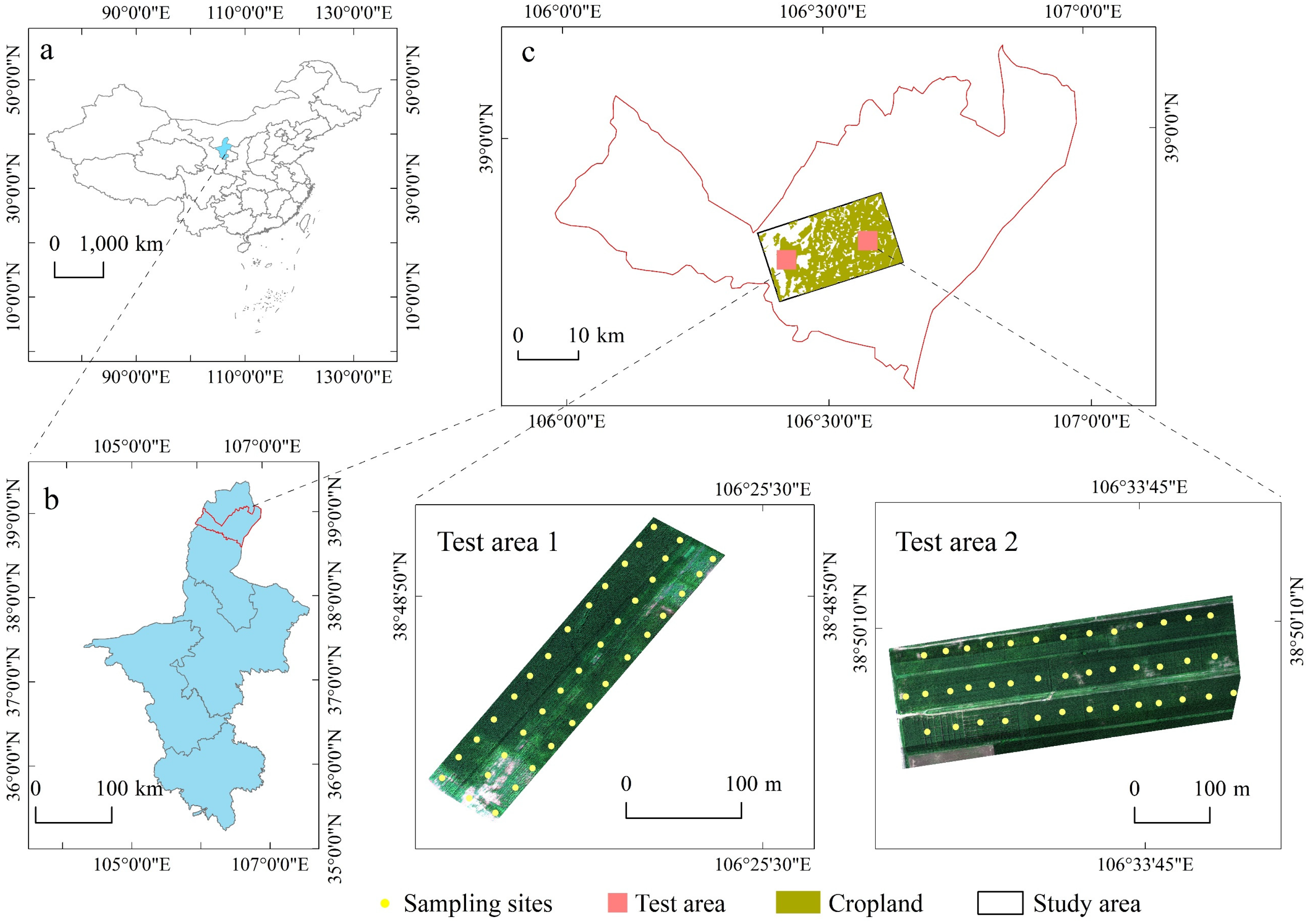
To achieve high-precision soil salinity monitoring over a wide area using satellites, this study employs several methods: dominant class variability weighting (DCVW), pixel aggregation (PA), nearest neighbor (NN), bilinear interpolation (BI), and cubic convolution interpolation (CCI). These methods were used to resample and upscale the UAV remote sensing data from a 0.2 m resolution to match the 10 m resolution of the Sentinel-2 satellite images. Two models were constructed: (1) UAV-Inversion (0.2 m): direct inversion model using the original high-resolution UAV data. (2) Upscaled UAV-Inversion (10 m): UAV data rescaled to 10 m resolution and used in the inversion model. Additionally, a separate model was created: (3) Satellite-Inversion (10 m): inversion model using Sentinel-2 satellite remote sensing data at a 10 m resolution. This study then selected the optimal method for upscaling UAV data, utilizing the Upscaled UAV-Inversion (10 m) model for numerical regression fitting with the Satellite-Inversion (10 m) model. This integrated approach combines the high-precision inversion capabilities of UAV remote sensing with the large-scale monitoring capabilities of satellite remote sensing. As a result, the combined model provides a more comprehensive and accurate inversion of large-scale soil salinity distribution.

The flowchart illustrating the sequence of these operations is presented in Figure 1.

2.1. Study Area

The study area is located in Pingluo County (38°26′60″~39°14′09″ N, 105°57′40″~106°52′52″ E), Ningxia Province, China (Figure 2). It is situated within a temperate arid desert climate zone, characterized by low precipitation (150–203 mm) and high evaporation (1825 mm). Xidatan Township is located in a saucer-shaped depression with low terrain and inadequate drainage conditions. Combined with intense evaporation, this geographical setting fosters salt accumulation, resulting in extensively saline soils. Qukou Township, situated in the Yellow River irrigation area, faces challenges from inefficient irrigation practices that often involve excessive diversion of water from the Yellow River for flood irrigation. Leakage during irrigation contributes to rising groundwater levels, while high evaporation rates further exacerbate soil salinization issues. Experimental areas were established within the cultivated lands of Xidatan Township and Qukou Township (Figure 2). The region’s cultivated crop is salt- and alkali-tolerant corn. The delineation of cultivated land was based on land use data provided by the Resources and Environmental Science Data Center of China (http://www.resdc.cn accessed on 21 November 2023).

2.2. Data Processing

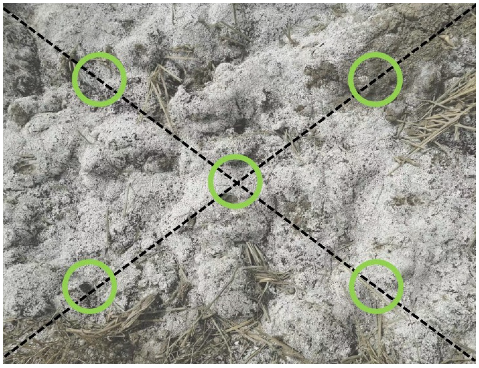
2.2.1. Soil Sample Collection and Preprocessing

Sampling sites were distributed as shown in Figure 2. Samples were collected from a depth of 0 to 20 cm surface soil. Sampling was performed using the five-point method (Figure 3).

A handheld GPS locator was used to determine the location of the sampling point that will serve as the center sampling point. Four points on its diagonal were selected at a distance of 1 m from the center sampling point. Soil samples from these five points are mixed and approximately 500 g of soil is taken as the final soil sample data for that sampling point. The soil samples underwent natural air-drying, grinding, and sieving through a 2 mm mesh. Prepared in a 1:5 water-soil ratio, the electric conductivity (EC) of the solution was determined. The soil salinity was calculated according to the empirical formula [28]. The formula was calculated as follows:

S = 2.357 EC_1:5 + 0.097

(1)

where S is the soil salinity in g·kg⁻¹ and EC_1:5 is the electrical conductivity of the soil aqueous solution, measured at a soil-to-water ratio of 1:5 in dS·m⁻¹. The conversion factor is 2.357 (g·kg⁻¹)/(dS·m⁻¹). It means that for every 1 dS·m⁻¹ increase in soil conductivity, the soil salinity increases by 2.357 g·kg⁻¹. A constant term used to adjust the offset of the formula is 0.097. That is, when the soil conductivity is 0, there is also 0.097 g·kg⁻¹ of soil salinity.

Each sample was tested three times, and the average value was recorded as the salinity for this location. Subsequently, samples were divided into modeling and validation sets at a ratio of 2:1 based on salinity. Salinity was classified into five levels [24,29]: non-saline (0~2 g·kg⁻¹), slightly saline (2~4 g·kg⁻¹), moderately saline (4~6 g·kg⁻¹), strongly saline (6~10 g·kg⁻¹), and extremely saline (>10 g·kg⁻¹).

2.2.2. Satellite Data Processing

The Sentinel-2 satellite image data for this study were obtained from the ESA Copernicus Data Center (https://scihub.copernicus.eu, accessed on 21 November 2023). The image was taken on 25 July 2022, with cloud cover below 5%. The images have been radiometrically calibrated and atmospherically corrected. Data resampling and format conversion were first performed using the Sentinel Application Platform (SNAP), and the resampled Sentinel-2 satellite multispectral image had a spatial resolution of 10 m in four bands (blue, green, red, and near-infrared) and a spectral range of 450–900 nm. After that, ENVI 5.6 was used for image cropping, stitching and other processing. Finally, the latitude and longitude information of the ground sampling points were imported into ArcGIS to obtain the corresponding surface spectral reflectance of each sampling point.

2.2.3. UAV Data Processing

The UAV hyperspectral data collection was conducted using a DJI Matrice M600 Pro hexacopter (DJ-Innovations, Shenzhen, China) equipped with a TwinLiHarmonic GaiaSky-mini push-broom hyperspectral imager. This operation occurred on 25 July 2022 within the designated test area at an altitude of 100 m. The hyperspectral imager covered wavelengths ranging from 386~1022 nm, with a spectral resolution of 5 nm and a spatial resolution of 0.2 m. Data acquisition took place between 11:00–14:00 on a sunny day with stable sunlight. Prior to takeoff, the sensors underwent calibration for dark current and white balance.

To align the spectral information from the UAV hyperspectral data with Sentinel-2 multispectral images, the UAV narrow-band spectral data were transformed into broad-band spectral data that corresponded to the satellite images. This transformation was accomplished through convolution operations utilizing the spectral response function characteristic of the satellite images [30,31]. The calculation formula used is as follows:

$${\rho }_s={\displaystyle \frac{{\int }_{{\lambda }_{max}}^{{\lambda }_{min}}s\left(\lambda \right)\rho \left(\lambda \right)d\lambda }{{\int }_{{\lambda }_{max}}^{{\lambda }_{min}}s\left(\lambda \right)d\lambda }}$$

(2)

where ${\rho }_{\mathrm{s}}$ is the hyperspectral fit to the satellite band reflectance, $s\left(\mathrm{\lambda }\right)$ is the satellite spectral response function, ${\lambda }_{min}$ and ${\lambda }_{max}$ are the maximum and minimum wavelengths of the band, and $\rho \left(\lambda \right)$ is the UAV hyperspectral data.

2.3. Methods

2.3.1. Upscaling Conversion Methods and Effects Evaluation

Nearest neighbor (NN) is a simple upscaling algorithm. It assigns the nearest pixel value to the image position to the corresponding position of the low-resolution image after upscaling. The calculations are performed sequentially in this way, thus realizing the upscaling conversion of the image.

Bilinear interpolation (BI) is a conventional method employed to interpolate pixel values by computing a weighted average based on neighboring pixels [32].

Cubic convolution interpolation (CCI) involves a distance-weighting operation applied to the pixel values of the surrounding 16 points. The calculated values are subsequently assigned as the pixel values for corresponding positions in the low-resolution image post-conversion [33].

Pixel aggregation (PA) involves combining pixel values within a moving window to derive the mean value through aggregation. All pixel values contributing to the output pixel within a specified range are weighted based on the scale factor [34].

Dominant class variability weighting (DCVW) determines the dominant eigenvalue based on the frequency of occurrence of values within a local trend surface. Initially, the variance of this dominant eigenvalue is computed for each image element in the local trend surface. Subsequently, the inverse of the variance is calculated and summed across all elements, yielding a cumulative value. Each image element’s weight is then determined by dividing its inverse variance by this cumulative value. Finally, the value of each pixel in the local trend surface is multiplied by its corresponding weight and summed, resulting in the weighted average of the local window trend surface [19]. This method utilizes statistical properties to emphasize the most significant variations in the local spatial context, enhancing the interpretation and representation of the trend surface. The calculation is as follows:

$$\begin{array}{c}{\widehat{y}}^{\left(w\right)x}={\displaystyle \sum _{u=1}^m}w\left(u\right)y\left(u\right)\end{array}$$

(3)

where

$$w\left(u\right)={\displaystyle \frac{\frac{1}{{\left(y\left(u\right)-y^{\left(wd\right)}\right)}^2}}{{\sum }_{u=1}^m\frac{1}{{\left(y\left(u\right)-y^{\left(wd\right)}\right)}^2}}}$$

(4)

and where ${\widehat{\mathrm{y}}}^{\left(\mathrm{w}\right)\mathrm{x}}$ is the window weighted average, w(u) is the pixel weight, y(wd) is the window dominant class value, and m is the number of pixels.

2.3.2. Calculation of Spectral Indices

The vegetation indices and salinity indices derived from various combinations of wavelengths in remote sensing images have shown promising results in salt monitoring [35,36]. This study focuses on 5 vegetation indices and 5 salinity indices selected for analysis (

Table 1. Spectral index calculation formulas.

Acronym	Spectral Index	Formula	Reference
S1	Salinity Index I	B/R	[37]
S2	Salinity Index II	(B − R)/(B + R)	[37]
S3	Salinity Index III	(G × R)/B	[37]
SI1	Salinity Index 1	(G × R)1/2	[38]
SI2	Salinity Index 2	(G2 + R2 + NIR2)1/2	[38]
NDVI	Normalized Difference Vegetation Index	(NIR − R)/(NIR + R)	[39]
NDSI	Normalized Difference Salinity Index	(R − NIR)/(R + NIR)	[40]
DVI	Difference Vegetation Index	NIR − R	[41]
GNDVI	Normalized Green Difference Vegetation Index	(NIR − G)/(NIR + G)	[42]
RDVI	Renormalized Difference Vegetation Index	(NIR − R)/(NIR + R)1/2	[42]

B, G, R, and NIR correspond to reflectance in blue (450~520 nm), green (540~580 nm), red (650~680 nm), and near-infrared (780~900 nm), respectively.

).

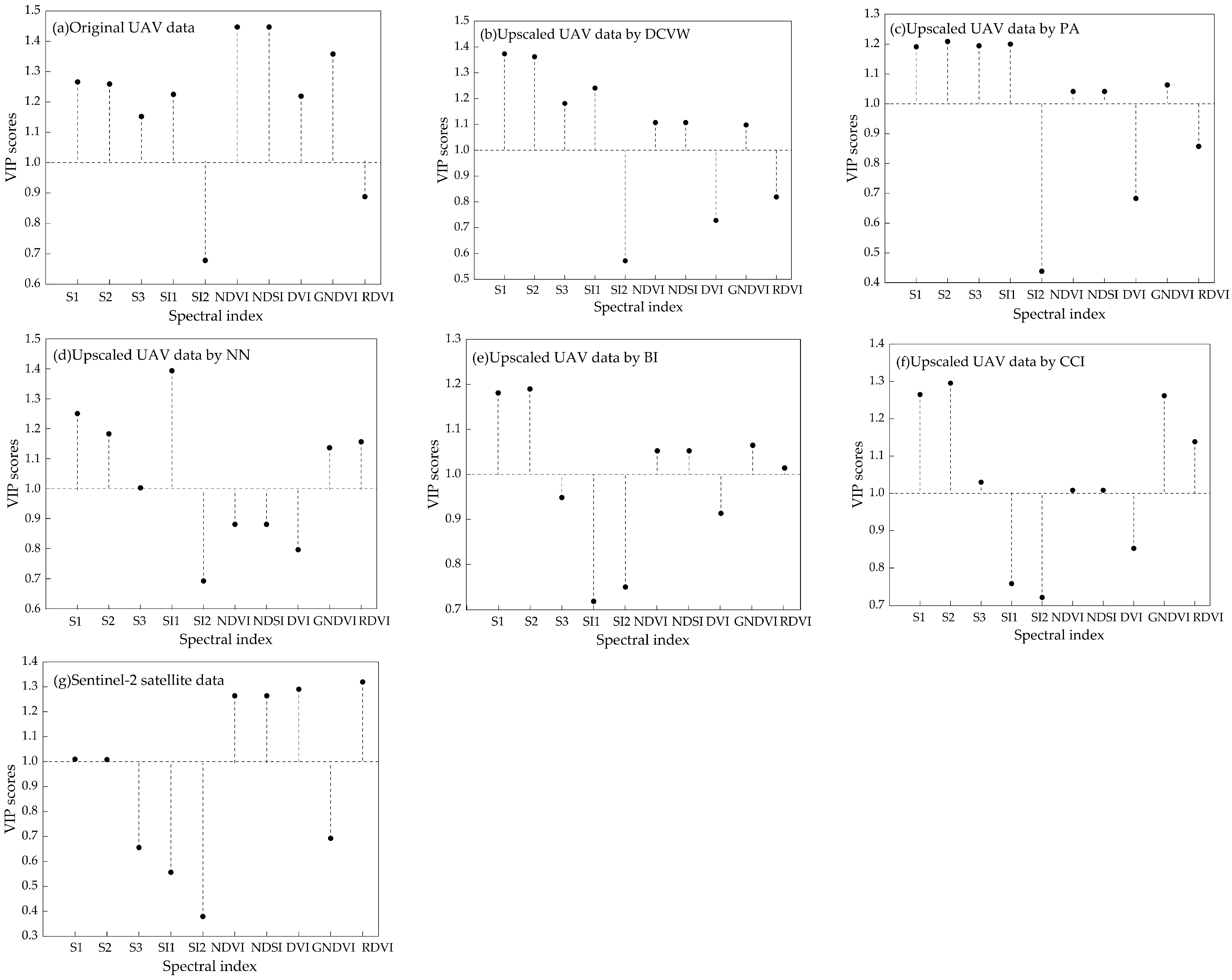
2.3.3. Features Selection

Sensitive spectral index screening was performed using the variable importance projection analysis (VIP). The VIP is a variable screening method based on partial least squares regression (PLSR) [43]. For a given independent variable, the VIP value not only represents the effect of the independent variable on the dependent variable but also considers the indirect influence of other independent variables on the dependent variable. The calculation of the VIP is:

$$\begin{array}{c}{VIP}_j=\sqrt{{\displaystyle \frac{p\times {\sum }_{f=1}^F{SSY}_f\times {W_{jf}}^2}{{SSY}_{total}\times F}}}\end{array}$$

(5)

where VIP_j is the importance of the j variable, p is the number of independent variables, F is the total number of principal components, f is the principal component, SSY_f is the sum of squared variances explained by the f principal component, SSY_total is the sum of squares of dependent variables, and W_jf² represents the importance of the j variable in the f principal component. The larger the VIP_j value, the stronger the explanatory power of the independent variable on the dependent variable. When the VIP value of an independent variable is greater than 1, it is considered an important independent variable.

2.3.4. Construction and Evaluation of the Soil Salinity Monitoring Model

Random forest (RF) is an ensemble learning algorithm that improves predictive performance by constructing multiple decision trees and aggregating their predictions [44]. It has shown effectiveness in accurately estimating soil salinity and major ions in arid regions [27].

Bayesian optimization [45] is a global optimization technique that relies on probabilistic models. It enhances model performance by constructing a probabilistic model of the objective function to identify the optimal hyperparameters. Three parameters that are indispensable for reducing content loss and determining the complexity and size of the decision tree were selected: maximum depth of the decision tree (max_depth), number of decision trees (n_estimators), and minimum number of samples for internal splitting (min_samples_split). Utilizing the BayesOpt optimizer facilitates hyperparameter optimization, thereby improving the model’s estimation accuracy and stability.

In this study, two widely adopted metrics, the coefficient of determination (R²) and root mean square error (RMSE), were selected to quantitatively assess and compare the accuracy of various soil salinity models. A higher R² value approaching 1 indicates a stronger correlation between predicted and actual values, reflecting better model performance. Conversely, a smaller RMSE value indicates less deviation of predicted values from actual observations, indicating higher precision in model predictions. Thus, in evaluating different soil salinity models, achieving R² values closer to 1 and minimizing RMSE values are indicative of higher accuracy and reliability.

2.3.5. Numerical Regression Method

Numerical regression was employed to establish a quadratic polynomial fitting function between satellite data and UAV data, aiming to determine their transformation relationship based on their correlation. Subsequently, this fitting function was utilized to correct the satellite remote sensing data. The regression fitting equation is shown below [46]:

A_i′ = a × A_i² + b × A_i + c

(6)

where a, b is the data conversion coefficient, c is the conversion residual, A_i is the data to be corrected, and A_i′ is the corrected data.

3. Results

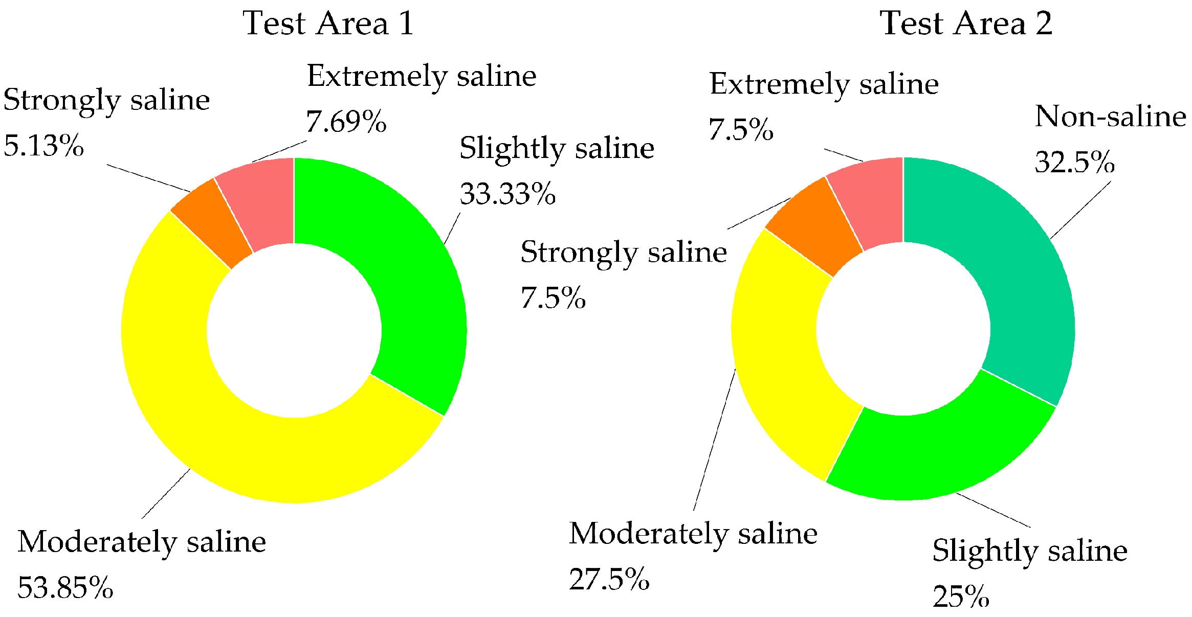
3.1. Statistical Characterization of Soil Salinity

The descriptive statistics of the samples in the test area are shown in

Table 2. Statistics of soil samples in the test areas.

Test	Sample Number	Salinity/g·kg−1
		Minimum	Maximum	Mean
Test Area 1	39	2.06	12.31	4.89
Test Area 2	40	0.41	18.37	4.18

. The soil salinity of the sample sites in Test Area 1 ranged from 2.06 g·kg⁻¹ to 12.31 g·kg⁻¹, with a mean value of 4.89 g·kg⁻¹. The soil salinity of the sample sites in Test Area 2 ranged from 0.41 g·kg⁻¹ to 18.37 g·kg⁻¹, with a mean value of 4.18 g·kg⁻¹. Figure 4 shows the graded distribution of soil salinity in the sample sites of each test area. Test Area 1 predominantly consisted of slightly and moderately saline soils, whereas Test Area 2 primarily included non-saline, slightly saline, and moderately saline soils.

3.2. Spectral Characteristics of Images after Upscaling by Different Methods

DCVW, PA, NN, BI, and CCI were utilized to resample the UAV images within the test areas, upscaling them to 10 m. The results of this scaling transformation in Test Area 2 are illustrated in Figure 5. Reflectance change was employed to quantitatively evaluate the effectiveness of the upscaling transformation, as shown in Figure 6. Overall, after employing the five upscaling methods on the UAV images, it was observed that the reflectance deviated minimally from the original images. This underscores the effectiveness of these methods in preserving overall image features and spectral information. Specifically, the images upscaled using PA and DCVW exhibited a high degree of consistency with the original images. This suggests that PA and DCVW are proficient in retaining detailed information and spectral properties during image reconstruction. Conversely, the images upscaled with NN, BI, and CCI displayed significant deviations from the original images. These methods may result in the loss or blurring of image details, indicating greater information loss. Hence, selecting an appropriate upscaling method is crucial for maintaining image quality and preserving information integrity, especially in applications requiring the precise reflection of spectral characteristics.

Furthermore, it was observed that the extent of changes in the images varied across different bands after upscaling using the five methods. In the blue band (450~520 nm), green band (540~580 nm), and red band (650~680 nm), the differences between the upscaled images and the original images were minimal. However, significant variations were noticeable in the near-infrared band (780~900 nm), where distinct magnitudes of changes were observed in the images after upscaling with different methods. This may be because the near-infrared band typically exhibits high sensitivity to the vegetation physiological status and surface moisture content. Different upscaling methods can affect the inter-band ratio relationships or the degree of detail preservation. Therefore, in the near-infrared band, the variations in image changes caused by various upscaling methods are more pronounced.

3.3. Optimal Factor Selection for Soil Salinity Inversion

The raw UAV hyperspectral data and the upscaled UAV hyperspectral data were resampled to multispectral using convolutional operations with different methods. The spectral indices were computed for various remote sensing data sources. For the seven types of remote sensing data sources, the number of independent variables selected from 10 spectral indices using the VIP were 8, 7, 7, 6, 6, 7, and 6, respectively, as shown in Figure 7.

3.4. Model Establishment

Using the parameters identified through the VIP screening as the independent variables and the soil salinity values as the dependent variables, RF models were constructed to quantitatively invert soil salinity. These models included the original UAV salinity inversion model, the original satellite salinity inversion model, and the UAV salinity inversion model after upscaling using different methods.

The hyperparameter optimization of these models employed a Bayesian algorithm. Considering the dataset size, the decision tree’s max_depth was varied from 1 to 20, n_estimators ranged from 1 to 100, and min_samples_split ranged from 2 to 25. The algorithm was iterated 100 times to identify the optimal combination of hyperparameters.

As an example, during the hyperparameter search process for the satellite salinity inversion model, the Bayesian optimization yielded optimal results with max_depth = 10, n_estimators = 31, and min_samples_split = 11, achieving the best R² (Figure 8). Thus, (10, 31, 11) was identified as the optimal hyperparameter combination for the satellite inversion model. The optimal hyperparameters for the different models are detailed in

Table 3. Optimal hyperparameter combinations of RF.

Data Sources	Characteristic Variable	Max_ Depth	N_ Estimators	Min_Samples _Split	R2
Original UAV data	S1, S2, S3, SI1, NDVI, NDSI, DVI, GNDV	10	33	9	0.893
Upscaled UAV data by DCVW	S1, S2, S3, SI1, NDVI, NDSI, GNDV	9	32	8	0.858
Upscaled UAV data by PA	S1, S2, S3, SI1, NDVI, NDSI, GNDV	11	29	2	0.817
Upscaled UAV data by NN	S1, S2, SI1, GNDV, DVI, RDVI	10	27	3	0.738
Upscaled UAV data by BI	S1, S2, NDVI, NDSI, GNDV, RDVI	8	31	12	0.744
Upscaled UAV data by CCI	S1, S2, S3, NDVI, NDSI, GNDV, RDVI	12	33	3	0.794
Sentinel-2 satellite data	S1, S2, NDVI, NDSI, DVI, RDVI	10	31	11	0.630

R² is the coefficient of determination.

.

Based on the model inversion results presented in

Table 4. Inverse modelling of soil salinity by different data sources.

Data Sources	Modeling Set		Validation Set
	R2	RMSE (g·kg−1)	R2	RMSE (g·kg−1)
Sentinel-2 satellite data	0.653	2.834	0.630	2.255
Original UAV data	0.853	1.844	0.893	1.448
Upscaled UAV data by DCVW	0.829	1.991	0.858	1.669
Upscaled UAV data by PA	0.762	2.349	0.817	1.897
Upscaled UAV data by NN	0.712	2.582	0.738	2.270
Upscaled UAV data by BI	0.702	2.628	0.744	2.242
Upscaled UAV data by CCI	0.836	1.948	0.794	2.010

R² is the coefficient of determination; RMSE is the root mean square error.

, it is evident that the R² of the UAV inversion model surpasses that of the satellite inversion model. Specifically, the UAV inversion model achieves an R² of 0.853 for the training set and 0.893 for the validation set, highlighting its robust fitting and generalization capabilities. In contrast, the satellite inversion model exhibits a lower R² of only 0.630, indicating a requirement for enhancement in estimation accuracy.

Among the UAV inversion models upscaled using various methods, the model upscaled by DCVW achieves the highest R² value of 0.858 and an RMSE of 1.669 g·kg⁻¹. The models upscaled by PA and CCI have R² values around 0.8, whereas the model upscaled by BI achieves an R² of 0.744. The model upscaled by NN exhibits the lowest R² at 0.738.

3.5. Calibration and Validation of Satellite Inversion Model for Soil Salinity

The UAV soil salinity inversion model upscaled using DCVW demonstrated the highest R² and was subsequently employed to correct the satellite soil salinity inversion model. Numerical regression was utilized to establish a fitting equation between the upscaled UAV soil salinity inversion data and the satellite inversion data, yielding the following equation:

$$\begin{array}{c}y=-0.02x^2+1.090x+0.297\end{array}$$

(7)

where y is the UAV soil salinity inversion value and x is the Sentinel-2 image soil salinity inversion value.

The satellite soil salinity inversion model from Table 4 was incorporated into Equation (7) as the independent variable to derive the corrected model and salt estimates. The corrected salinity estimates were fitted to the measured soil salinity (Figure 9). The results showed that the R² of the corrected satellite soil salinity inversion model improved from 0.630 to 0.787. The regression line between the measured and inverted values approaches 1:1 more closely, demonstrating that the upscaling conversion correction effectively enhances the accuracy of soil salinity inversion in satellite imagery.

Model validation was conducted by assessing the consistency of the soil salinity distribution derived from the satellite data before and after correction with the upscaled UAV-derived soil salinity distribution. Using Test Area 2 as an example, Figure 10a shows the soil salinity distribution map obtained by inversion based on the original UAV image. Figure 10b presents the soil salinity distribution map obtained from the UAV data after upscaling using the DCVW method. Figure 10c depicts the soil salinity distribution map derived directly from the raw satellite images. Figure 10d illustrates the soil salinity distribution map obtained by correcting the satellite soil salinity inversion model using the UAV data.

The comparison in

Table 5. Similarity rates before and after calibration of UAV soil salinity inversion model and satellite soil salinity inversion model (%).

Degree of Salinization	Non-Saline	Slightly Saline	Moderately Saline	Strongly Saline	Extremely Saline
Pre-correction	90.747	57.272	55.698	80.940	94.200
Post-correction	95.389	90.335	76.126	94.866	97.153

reveals significant differences between Figure 10b,c, with a mean similarity rate of 75.771% across the different salinization levels. In contrast, Figure 10d exhibits a much higher consistency with Figure 10b, showing a mean similarity rate of 90.774% across the different salinization levels. This indicates that the upscaled inversion model effectively enhances the accuracy of the soil salinity inversion.

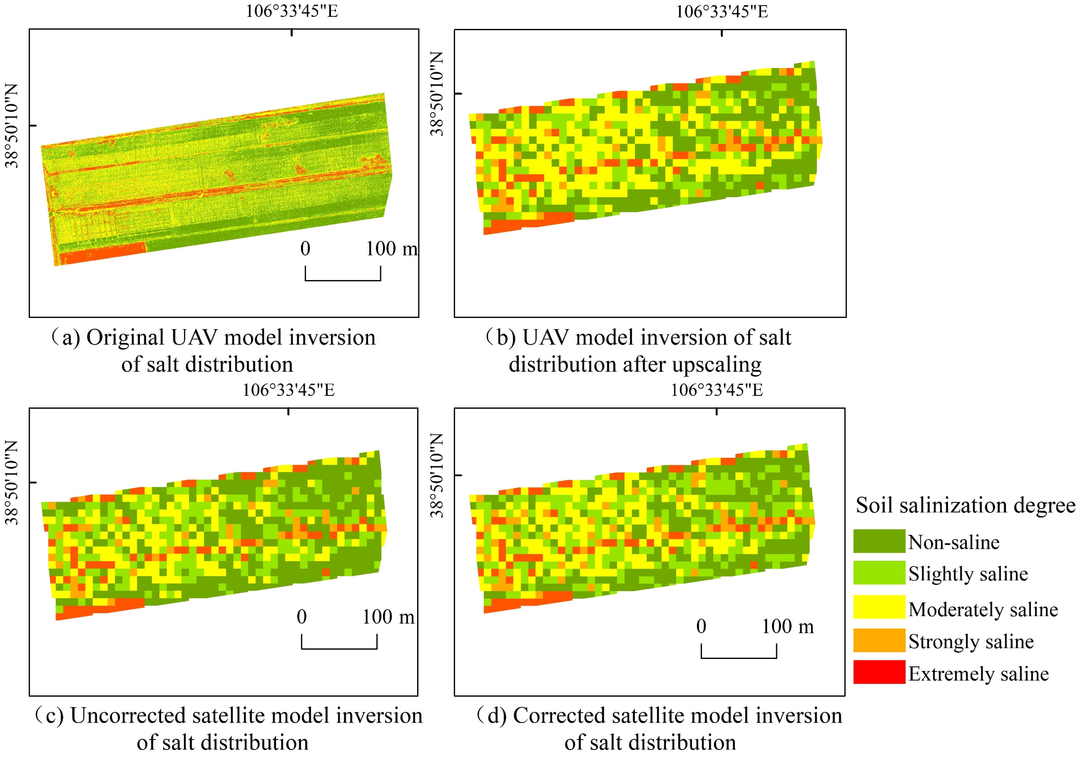
3.6. Model Application

The inversion of the soil salinity distribution in arable land within the study area, using the corrected satellite soil salinity model (Figure 11), emphasizes a substantial salinization of the cultivated land in central Pingluo County. This region is primarily characterized by slightly and moderately saline soils. In contrast, areas with non-saline, strongly saline, and extremely saline soils are dispersed across the study area, encompassing the northern, central, and southern parts of the county.

4. Discussion

4.1. Enhancing Soil Salinity Monitoring Accuracy: Integrating UAV with Satellite Data

The UAV data used in this study has a spatial resolution of 0.2 m. The constructed soil salinity inversion model achieves an R² of 0.893 with an RMSE of 1.448 g·kg⁻¹, accurately reflecting the salinity of the individual image elements and closely matching the measured surface soil salinity distribution [47]. In contrast, although Sentinel-2 images offer wide coverage, their spatial resolution is only 10 m, making it challenging to achieve a precise alignment with actual ground sampling points. The model’s R² is only 0.630, with an RMSE of 2.255 g·kg⁻¹. In previous studies [48], the soil salinity in the test area obtained from the best model inversion of the UAV data was often “averaged out” as the “true value of salinity” for satellite data modeling. The approach has led to marginal improvements in satellite model accuracy due to the spatial heterogeneity of soil salinity. Averaging the image element information at small regional scales weakens the autocorrelation and heterogeneity of the surface salinity information, resulting in deviations from the actual conditions [49]. In addition, Zhang et al. (2019) [50] directly used UAV data to calibrate the satellite model, and Zhu et al. (2021) [51] used UAV data and Sentinel-2 data together as the input independent variables to construct a model, both of which ignored the problem of mismatch between the two spatial scales. On the basis of maintaining the local detail features of the remote sensing data, image data resampling upscaling can better maintain the information content and spatial structure features of the original remote sensing data [21,52]. Therefore, in this study, the upscaling of the UAV data was converted to the same pixel scale as the satellite images, and then the satellite–machine data fusion correction was carried out to realize the large-scale and high-precision soil salinity inversion of the satellite data.

In addition, comparing the satellite inversion salinity distribution maps before and after correction with the UAV inversion salinity distribution maps, it was found that the accuracy was significantly improved. The rate of identity of the results with the real soil salinity distribution increased from 75.771% before correction to 90.774% after correction. The uncorrected satellite model has a lower rate of identity at mild and moderate salinity levels due to the surface heterogeneity and the presence of salinity underestimation and overestimation in the satellite inversion process [53,54]. After correction, the identical rates were increased to 90.335% and 76.126%, respectively, which greatly reduced the influence of surface heterogeneity on the inversion accuracy. Therefore, this study further verifies that the correction of satellite data using UAV data can effectively improve the accuracy of the satellite inversion model. Figure 10 shows that the salinity inversion grading distribution results are more consistent with the field sampling results. This indicates that the method of fusion of UAVs and satellites to improve the accuracy of satellite inversion models is universal and can be applied to a wider range. However, due to the large difference in the geographic environment of different regions, the model inversion accuracy will be different in different regions (inland arid zone and coastal humid zone). The optimization of the model hyperparameters needs to be carried out according to the soil properties.

4.2. Improving the Accuracy of Soil Salinization Assessments by Selecting Appropriate Upscaling Methods

The heterogeneity of the surface space seriously affects the conversion of spatial scales [12]. As shown by the measured salinity data and the inversion results from different experimental areas, the surface salinity information was unevenly distributed in the study area (Figure 4 and Figure 11). Therefore, a suitable scale conversion method is crucial for the accurate assessment of salinity information [55]. This study compared the traditional resampling upscaling method with DCVW and found that DCVW was the most effective, followed by PA, BI, and CCI. NN had the lowest accuracy. The NN method simply selects the spatially closest original image element as the value of the new image element without weighting. In contrast, BI predicts the image element values on the new scale by averaging the neighboring image elements. CCI can reduce the loss of high-frequency information and the heterogeneity of images [22]. PA also preserves the detailed features in the image by aggregating the information of neighboring pixels. However, for high-resolution images, this method may also lead to the loss of some detailed information. However, DCVW not only weights the image elements in the upscaling process but also fully considers the heterogeneity of the surrounding image elements and adapts to the changes in different regions [56]. Zhang et al. (2022) [15] also found that DCVW has an absolute advantage in star-machine scale change. Compared to the traditional resampling upscaling method, DCVW is able to simultaneously consider the contributions of multiple variables to the overall variation and is able to determine which spectral bands or environmental variables have the greatest impact on the soil salinity distribution. Local soil information can be retained more effectively during the scale conversion process, which improves the accuracy of the analysis results. It is suitable for extracting soil salinity information with spatial heterogeneity.

4.3. Spectral Matching between UAV Hyperspectral and Satellite Multispectral Data

In studies comparing satellite–UAV spectral matching, UAV multispectral data is predominantly utilized. However, the wavelength ranges and central wavelengths of UAV multispectral data often differ from those of satellite multispectral data. This discrepancy can result in some spectral information being overlooked when combining UAV and satellite images, thereby impacting the inversion accuracy [18,57]. Hyperspectral sensors typically capture hundreds of contiguous spectral bands with narrow bandwidths, allowing for flexible band combinations that can align with the wavelength ranges of satellite multispectral bands [58]. Therefore, correcting satellite multispectral data using UAV hyperspectral data tends to achieve higher accuracy in correction processes [59].

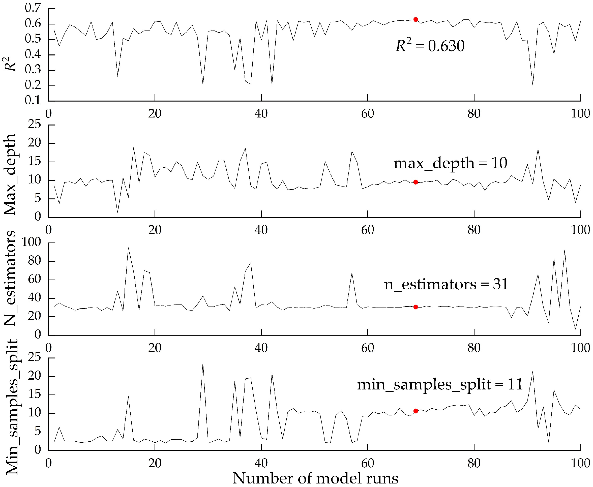
4.4. Hyperparametric Optimization of RF

The selection of hyperparameters is crucial in the application of machine learning algorithms. The effectiveness of RF inversion depends on choosing an appropriate set of hyperparameters. Additionally, many previous studies employed grid search or random search methods [60]. Grid search, which exhaustively explores the parameter space, is often inefficient and impractical. Conversely, random search may overlook the optimal solution [61]. The Bayesian optimization of hyperparameters offers a solution to these challenges by avoiding arbitrary value selection, reducing search time, and addressing the black-box nature of RF models [45].

4.5. Research Limitations and Future Work

We observed that the inversion accuracy of the models derived from the UAV data diminished after upscaling using various methods compared to the original UAV model’s accuracy. This reduction is primarily due to spatial heterogeneity, where resampling leads to inevitable feature distortion and loss of spectral information [62,63,64], thereby compromising the final results. Qiu et al. (2023) [65] introduced a deep learning model, Res-Transformer, based on the surface reflectance scale transformation of UAV images, which demonstrated superior accuracy and robustness over traditional scale transformation methods. In another study, Wang et al. (2021) [66] utilized RF, KNN, and Cubist machine learning algorithms to upscale site-scale albedo to the image scale, achieving high-quality, spatiotemporally continuous image-scale reference values. Future research should therefore explore the integration of machine learning and other advanced algorithms to minimize errors in UAV–satellite scale conversion and enhance the accuracy of UAV–satellite upscaling for soil salinity inversion.

Additionally, Ge et al. (2022) [67] identified environmental covariates influencing soil salinity, including spectral information, soil saline indices, DEM, temperature, soil moisture information, precipitation, NDVI, and land cover. Wang et al. (2022) [68] found that the degree of soil salinization was influenced by factors such as topography, climate, and water table depth, and showed significant changes in different seasons. Among them, soil salinity was higher in the dry season (April) than in the wet season (October). This may be due to the fact that evaporation is much greater than precipitation during the dry season, resulting in the convergence of surface salts. In contrast, during the wet season, precipitation is greater than evaporation, resulting in the dissolution of surface salts and a reduction in surface salts. It can be seen that temporal transformation and soil depth are also important factors influencing salinity distribution.

This paper only studied the distribution of salinity in the surface layer of the soil, which may have some bias. Therefore, subsequent studies should consider the environmental changes in different seasons and introduce more environmental covariates to invert the soil salinity distribution. Moreover, microwave remote sensing has the ability to detect targets below the surface [69]. Future research could consider using UAVs equipped with microwave sensors to obtain soil salinity and remote sensing information at different depths (0–20 cm, 20–40 cm). The aim is to achieve higher precision, faster speed, and broader coverage in acquiring soil salinity information.

5. Conclusions

This study explores the application of UAV upscaling to correct satellite data, thereby enhancing the accuracy of satellite-based soil salinity monitoring. The findings indicate that utilizing UAV-upscaled and corrected satellite data effectively improves the precision of the satellite model inversion while expanding the scope of salinity monitoring.

The UAV-based remote sensing model for soil salinity inversion demonstrates higher accuracy compared to the satellite-based models. By employing upscaled UAV imagery to calibrate the satellite model, the R² value of the satellite inversion model improved from 0.630 to 0.787, and the RMSE decreased from 2.696 g·kg⁻¹ to 2.043 g·kg⁻¹. The validation of the corrected satellite inversion model using a UAV-derived salt distribution map showed an enhancement in the matching rate of salt distribution from 75.771% to 90.774%. This result underscores the model’s capability for high-precision inversion across a broad spectrum of soil salinity levels.

In conclusion, the UAV–satellite data fusion approach proposed in this study for soil salinity inversion provides valuable insights for large-scale, high-precision monitoring of soil salinity. This approach is essential for effective land management and agricultural practices in saline-affected areas.

References

1. Taghadosi, M.M.; Hasanlou, M.; Eftekhari, K. Retrieval of soil salinity from Sentinel-2 multispectral imagery. Eur. J. Remote Sens. 2019, 52, 138–154. [Google Scholar] [CrossRef]
2. Wang, Z.; Zhang, F.; Zhang, X.; Chan, N.W.; Kung, H.-T.; Ariken, M.; Zhou, X.; Wang, Y. Regional suitability prediction of soil salinization based on remote-sensing derivatives and optimal spectral index. Sci. Total Environ. 2021, 775, 145807. [Google Scholar] [CrossRef]
3. Wang, X.; Zhang, F.; Ding, J.; Kung, H.-T.; Latif, A.; Johnson, V.C. Estimation of soil salt content (SSC) in the Ebinur Lake wetland National Nature Reserve (ELWNNR), Northwest China, based on a bootstrap-BP neural network model and optimal spectral indices. Sci. Total Environ. 2018, 615, 918–930. [Google Scholar] [CrossRef]
4. Cerro, J.; Ulloa, C.; Barrientos, A.; Rivas, J. Unmanned Aerial Vehicles in Agriculture: A Survey. Agronomy 2021, 11, 203. [Google Scholar] [CrossRef]
5. Ivushkin, K.; Bartholomeus, H.; Bregt, A.K.; Pulatov, A.; Franceschini, M.H.D.; Kramer, H.; van Loo, E.N.; Jaramillo Roman, V.; Finkers, R. UAV based soil salinity assessment of cropland. Geoderma 2019, 338, 502–512. [Google Scholar] [CrossRef]
6. Wei, G.; Li, Y.; Zhang, Z.; Chen, Y.; Chen, J.; Yao, Z.; Lao, C.; Chen, H. Estimation of soil salt content by combining UAV-borne multispectral sensor and machine learning algorithms. PeerJ 2020, 8, e9087. [Google Scholar] [CrossRef]
7. Ge, X.; Ding, J.; Jin, X.; Wang, J.; Chen, X.; Li, X.; Liu, J.; Xie, B. Estimating Agricultural Soil Moisture Content through UAV-Based Hyperspectral Images in the Arid Region. Remote Sens. 2021, 13, 1562. [Google Scholar] [CrossRef]
8. Yu, X.; Chang, C.; Song, J.; Zhuge, Y.; Wang, A. Precise monitoring of soil salinity in China’s Yellow River Delta using UA V-borne multispectral imagery and a soil salinity retrieval index. Sensors 2022, 22, 546. [Google Scholar] [CrossRef]
9. Yan, D.; Li, J.; Yao, X.; Luan, Z. Integrating UAV data for assessing the ecological response of Spartina alterniflora towards inundation and salinity gradients in coastal wetland. Sci. Total Environ. 2022, 814, 631. [Google Scholar] [CrossRef]
10. Zhu, C.M.; Ding, J.L.; Zhang, Z.P.; Wang, Z. Exploring thepotential of UAV hyperspectral image for estimating soil salinity: Effects of optimal band combination algorithm and random forest. Spectrochim. Acta Part A Mol. Biomol. Spectrosc. 2022, 121, 416. [Google Scholar]
11. Emilien, A.V.; Thomas, C.; Thomas, H. UAV & satellite synergies for optical remote sensing applications: A literature review. Sci. Remote Sens. 2021, 3, 100019. [Google Scholar]
12. Qi, G.H.; Chang, C.Y.; Yang, W.; Gao, P.; Zhao, G.X. Soil salinity inversion in coastal corn planting areas by the satellite-UAV-ground integration approach. Remote Sens. 2021, 13, 3100. [Google Scholar] [CrossRef]
13. Zhang, S.; Zhao, G.; Lang, K.; Su, B.; Chen, X.; Xi, X.; Zhang, H. Integrated satellite, unmanned aerial vehicle (UAV) and ground inversion of the SPAD of winter wheat in the reviving stage. Sensors 2019, 19, 1485. [Google Scholar] [CrossRef] [PubMed]
14. Ma, Y.; Zhu, W.; Zhang, Z.; Chen, H.; Zhao, G.; Liu, P. Fusion level of satellite and UAV image data for soil salinity inversion in the coastal area of the Yellow River Delta. Int. J. Remote Sens. 2022, 43, 7039–7063. [Google Scholar] [CrossRef]
15. Zhang, Z.; Chen, Q.; Huang, X.; Song, Z.; Zhang, J.; Tai, X. UAV-Satellite Remote Sensing Scale-up Monitoring Model of Soil Salinity Based on Dominant Class Variability-weighted Method. Trans. Chin. Soc. Agric. Mach. 2022, 53, 226–238+251. [Google Scholar]
16. He, L.; Chen, W.; Leblanc, S.G.; Lovitt, J.; Arsenault, A.; Schmelzer, I.; Fraser, R.H.; Latifovic, R.; Sun, L.; Prévost, C.; et al. Integration of multi-scale remote sensing data for reindeer lichen fractional cover mapping in eastern Canada. Remote Sens. Environ. 2021, 267, 112731. [Google Scholar] [CrossRef]
17. Wu, W.; Al-Shafie, W.M.; Mhaimeed, A.S.; Ziadat, F.; Nangia, V.; Payne, W.B. Soil salinity mapping by multiscale remote sensing in Mesopotamia, Iraq. IEEE J. Sel. Top. Appl. Earth Obs. Remote Sens. 2014, 7, 4442–4452. [Google Scholar] [CrossRef]
18. Ma, Y.; Chen, H.; Zhao, G.X.; Wang, Z.R.; Wang, D.Y. Spectral index fusion for salinized soil salinity inversion using Sentinel-2A and UAV images in a coastal area. IEEE Access 2020, 8, 159595–159608. [Google Scholar] [CrossRef]
19. Wang, G.; Gertner, G.Z.; Anderson, A.B. Up-scaling methods based on variability-weighting and simulation for inferring spatial information across scales. Int. J. Remote Sens. 2004, 25, 4961–4979. [Google Scholar] [CrossRef]
20. Feng, W.Z.; Wang, X.T.; Han, J.; Zhao, Y.X.; Liang, L.; Li, D.Q.; Tang, X.X.; Zhang, Z.T. Research on soil salinization monitoring based on scale conversion of satellite and UAV remote sensing data. Shandong Univ. Sci. Technol. 2020, 11, 87–93. [Google Scholar]
21. Chen, J.Y.; Wang, X.T.; Zhang, Z.T.; Han, J.; Yao, Z.H.; Wei, G.F. Soil salinization monitoring method based on UAV-satellite remote sensing scale-up. Trans. Chin. Soc. Agric. Mach. 2019, 50, 161–169. [Google Scholar]
22. Chen, C.; Bao, Y.X.; Zhu, F.; Yang, R.M. Remote sensing monitoring of rice growth under Cnaphalocrocis medinalis (Guenée) damage by integrating satellite and UAV remote sensing data. Int. J. Remote Sens. 2024, 45, 772–790. [Google Scholar] [CrossRef]
23. Gao, Y.; Liang, Z.; Wang, B.; Wu, Y.; Shiyu, L. UAV and satellite remote sensing images based aboveground Biomass Inversion in the Meadows of Lake Shengjin. J. Lake Sci. 2019, 31, 517–528. [Google Scholar]
24. Zhang, Y.; Hou, K.; Qian, H.; Gao, Y.; Fang, Y.; Xiao, S.; Tang, S.; Zhang, Q.; Qu, W.; Ren, W. Characterization of soil salinization and its driving factors in a typical irrigation area of Northwest China. Sci. Total Environ. 2022, 837, 155808. [Google Scholar] [CrossRef] [PubMed]
25. Jia, P.P.; Zhang, J.H.; He, W.; Hu, Y.; Zeng, R.; Zamanian, K.; Jia, K.; Zhao, X. Combination of hyperspectral and machine learning to invert soil electrical conductivity. Remote Sens. 2022, 14, 2602. [Google Scholar] [CrossRef]
26. Wang, F.; Shi, Z.; Biswas, A.; Yang, S.T.; Ding, J.L. Multi-algorithm comparison for predicting soil salinity. Geoderma 2020, 365, 114211. [Google Scholar] [CrossRef]
27. Fathizad, H.; Ardakani, M.A.H.; Sodaiezadeh, H.; Kerry, R.; Taghizadeh-Mehrjardi, R. Investigation of the spatial and temporal variation of soil salinity using random forests in the central desert of Iran. Geoderma 2020, 365, 114233. [Google Scholar] [CrossRef]
28. Chen, R.H.; Wang, Y.J.; Zhang, J.H.; Shang, T.H. Inversion of soil salinity in Yinchuan Plain based on fractional-order differential spectral index. Chin. J. Ecol. 2023, 42, 2296–2304. [Google Scholar]
29. Ren, D.; Wei, B.; Xu, X.; Engel, B.; Li, G.; Huang, Q.; Xiong, Y.; Huang, G. Analyzing spatiotemporal characteristics of soil salinity in arid irrigated agro-ecosystems using integrated approaches. Geoderma 2019, 356, 113935. [Google Scholar] [CrossRef]
30. Wang, Q.; Tang, Y.; Ge, Y.; Xie, H.; Tong, X.; Atkinson, P.M. A comprehensive review of spatial-temporal-spectral information reconstruction techniques. Sci. Remote Sens. 2023, 8, 100102. [Google Scholar] [CrossRef]
31. Hu, J.; Peng, J.; Zhou, Y.; Xu, D.; Zhao, R.; Jiang, Q.; Fu, T.; Wang, F.; Shi, Z. Quantitative estimation of soil salinity using UAV-borne hyperspectral and satellite multispectral images. Remote Sens. 2019, 11, 736. [Google Scholar] [CrossRef]
32. Bovik, A.C. The Essential Guide to Image Processing; Academic Press: Cambridge, MA, USA, 2009; pp. 43–68. [Google Scholar]
33. Chen, Y.; Yang, R.; Zhao, N.; Zhu, W.; Huang, Y.; Zhang, R.; Chen, X.; Liu, J.; Liu, W.; Zuo, Z. Concentration Quantification of Oil Samples by Three-Dimensional Concentration-Emission Matrix (CEM) Spectroscopy. Appl. Sci. 2020, 10, 315. [Google Scholar] [CrossRef]
34. Wu, M.Q.; Niu, Z.; Wang, C.Y. Mapping paddy fields by using spatial and temporal remote sensing data fusion technology. Trans. Chin. Soc. Agric. Eng. 2010, 26, 48–52. [Google Scholar]
35. Ge, X.Y.; Wang, J.Z.; Ding, J.L.; Cao, X.Y.; Zhang, Z.P.; Liu, J.; Li, X.H. Combining UAV-based hyperspectral imagery and machine learning algorithms for soil moisture content monitoring. PeerJ 2019, 7, e6926. [Google Scholar] [CrossRef]
36. Han, Y.; Ge, H.; Xu, Y.; Zhuang, L.; Wang, F.; Gu, Q.; Li, X. Estimating soil salinity using multiple spectral indexes and machine learning algorithm in songnen plain, China. IEEE J. Sel. Top. Appl. Earth Obs. Remote Sens. 2023, 16, 7041–7050. [Google Scholar]
37. Abbas, A.; Khan, S. Using remote sensing techniques for appraisal of irrigated soil salinity. In Proceedings of the International Congresson Modelling and Simulation (MODSIM), Christchurch, New Zealand, 10–13December 2007; pp. 2632–2638. [Google Scholar]
38. Douaoui, A.E.K.; Nicolas, H.; Walter, C. Detecting salinity hazards within a semiarid context by means of combining soil and remote-sensing data. Geoderma 2006, 134, 217–230. [Google Scholar] [CrossRef]
39. Zhang, T.T.; Zeng, S.L.; Gao, Y.; Ouyang, Z.T.; Li, B.; Fang, C.M.; Zhao, B. Using hyperspectral vegetation indices as a proxy to monitor soil salinity. Ecol. Indic. 2011, 11, 1552–1562. [Google Scholar] [CrossRef]
40. Allbed, A.; Kumar, L.; Aldakheel, Y.Y. Assessing soil salinity using soil salinity and vegetation indices derived from IKONOS high-spatial resolution imageries: Applications in a date palm dominated region. Geoderma 2014, 230–231, 1–8. [Google Scholar] [CrossRef]
41. Dong, C.; Zhao, G.X.; Su, B.W.; Chen, X.N.; Zhang, S.M. Research on the Decision Model of Variable Nitrogen Application in Winter Wheat’s Greening Period Based on UAV Multispectral Image. Spectrosc. Spect. Anal. 2019, 39, 3599–3605. [Google Scholar]
42. Dong, J.J.; Niu, J.M.; Zhang, Q.; Kang Sa, R.L.; Han, F. Remote sensing yield estimation of typical grassland based on multi-source satellite data. Chin. J. Grassl. 2013, 35, 64–69. [Google Scholar]
43. Oussama, A.; Elabadi, F.; Platikanov, S.; Kzaiber, F.; Tauler, R. Detection of olive oil adulteration using FT-IR spectroscopy and PLS with variable importance of projection (VIP) scores. J. Am. Oil Chem. Soc. 2012, 89, 1807–1812. [Google Scholar] [CrossRef]
44. Wang, Z.Y.; Ding, J.L.; Tan, J.; Liu, J.H.; Zhang, T.T.; Cai, W.J.; Meng, S.S. UAV hyperspectral analysis of secondary salinization in arid oasis cotton fields: Effects of FOD feature selection and SOA-RF. Frontiers. Plant Sci. 2024, 15, 1358965. [Google Scholar] [CrossRef]
45. Shahriari, B.; Swersky, K.; Wang, Z.; Adams, R.P.; Freitas, N.D. Taking the human out of the loop: A review of Bayesian optimization. Proc. IEEE 2016, 104, 148–175. [Google Scholar] [CrossRef]
46. Miura, T.; Huete, A.; Yoshioka, H. An empirical investigation of cross-sensor relationships of NDVI and red/near-infrared reflectance using EO-1 Hyperion data. Remote Sens. Environ. 2006, 100, 223–236. [Google Scholar] [CrossRef]
47. Jia, J.D.; Chen, C.; Liu, Q.; Ding, B.B.; Ren, Z.; Jia, Y.X.; Bai, X.Q.; Du, R.Q.; Chen, Q.D.; Wang, S.; et al. Soil salinity monitoring model based on the synergistic construction of ground-UA-satellite data. Soil Use. Manag. 2024, 40, e12980. [Google Scholar] [CrossRef]
48. Qi, G.; Zhao, G.; Xi, X. Soil Salinity Estimation of Winter Wheat Areas Based on Satellite-Unmanned Aerial Vehicle-Ground Collaborative System in Coastal of the Yellow River Delta. Sensors 2020, 20, 6521. [Google Scholar] [CrossRef]
49. Hu, Z.; Miao, Q.; Shi, H.; Feng, W.; Hou, C.; Yu, C.; Mu, Y. Spatial Variations and Distribution Patterns of Soil Salinity at the Canal Scale in the Hetao Irrigation District. Water 2023, 15, 3342. [Google Scholar] [CrossRef]
50. Zhang, S.M.; Zhao, G.X. A Harmonious Satellite-Unmanned Aerial Vehicle-Ground Measurement Inversion Method for Monitoring Salinity in Coastal Saline Soil. Remote Sens. 2019, 11, 1700. [Google Scholar] [CrossRef]
51. Zhu, W.; Rezaei, E.E.; Nouri, H.; Yang, T.; Li, B.; Gong, H.; Lyu, Y.; Peng, J.; Sun, Z. Quick detection of field-scale soil comprehensive attributes via the integration of UAV and sentinel-2B remote sensing data. Remote Sens. 2021, 13, 4716. [Google Scholar] [CrossRef]
52. Xi, X.; Zhao, G.; Gao, P.; Cui, K.; Li, T. Inversion of soil salinity in coastal winter wheat growing area based on sentinel satellite and unmanned aerial vehicle multi-spectrum-A case study in Kenli district of the Yellow River delta. Sci. Agric. Sin. 2020, 53, 5005–5016. [Google Scholar]
53. Ding, J.L.; Yu, D.L. Monitoring and evaluating spatial variability of soil salinity in dry and wet seasons in the Werigan–Kuqa oasis, China, using remote sensing and electromagnetic induction instruments. Geoderma 2014, 235–236, 316–322. [Google Scholar] [CrossRef]
54. Zhang, Q.; Li, L.; Sun, R.; Zhu, D.; Zhang, C.; Chen, Q. Retrieval of the soil salinity from Sentinel-1 dual-polarized SAR data based on deep neural network regression. IEEE Geosci. Remote Sens. Lett. 2022, 19, 4006905. [Google Scholar] [CrossRef]
55. Wang, J.Z.; Ding, J.L.; Yu, D.L.; Teng, D.X.; He, B.; Chen, X.Y.; Ge, X.Y.; Zhang, Z.P.; Wang, Y.; Yang, X.D.; et al. Machine learning-based detection of soil salinity in an arid desert region, Northwest China: A comparison between Landsat 8 OLI and Sentinel 2 MSI. Sci. Total Environ. 2020, 707, 136092. [Google Scholar] [CrossRef]
56. Guo, Z.Q.; Li, X.; Ren, Y.S.; Qian, S.J.; Shao, Y.R. Research on regional soil moisture dynamics based on hyperspectral remote sensing technology. Int. J. Low Carbon Technol. 2023, 18, 737–749. [Google Scholar] [CrossRef]
57. Hu, K.; Wang, S.; Li, H.; Huang, F.; Li, B. Spatial scaling effects on variability of soil organic matter and total nitrogen in suburban Beijing. Geoderma 2014, 226–227, 54–63. [Google Scholar] [CrossRef]
58. Sun, M.; Li, Q.; Jiang, X.; Ye, T.; Li, X.; Niu, B. Estimation of soil salt content and organic matter on arable land in the Yellow River Delta by combining UAV hyperspectral and Landsat-8 multispectral imagery. Sensors 2022, 22, 3990. [Google Scholar] [CrossRef] [PubMed]
59. Zhu, W.X.; Sun, Z.G.; Yang, T.; Li, J.; Peng, J.B.; Zhu, K.Y.; Li, S.J.; Gong, H.R.; Lyu, Y.; Li, B.B.; et al. Estimating leaf chlorophyll content of crops via optimal unmanned aerial vehicle hyperspectral data at multi-scales. Comput. Electron. Agric. 2020, 178, 105786. [Google Scholar] [CrossRef]
60. Shams, M.Y.; Elshewey, A.M.; El-kenawy, E.S.M.; Ibrahim, A.; Talaat, F.M.; Tarek, Z. Water Quality Prediction Using Machine Learning Models Based on Grid Search Method. In Multimedia Tools and Applications; Springer: Berlin/Heidelberg, Germany, 2023. [Google Scholar]
61. Stuke, A.; Rinke, P.; Todorovic, M. Efficient Hyperparameter Tuning for Kernel Ridge Regression with Bayesian Optimization. Mach. Learn. Sci. Technol. 2021, 2, 035022. [Google Scholar] [CrossRef]
62. Li, R.; Gao, X.; Shi, F.; Zhang, H. Scale Effect of Land Cover Classification from Multi-Resolution Satellite Remote Sensing Data. Sensors 2023, 23, 6136. [Google Scholar] [CrossRef] [PubMed]
63. Zhang, X.; Zuo, W.; Zhao, S.; Jiang, L.; Chen, L.; Zhu, Y. Uncertainty in Upscaling In Situ Soil Moisture Observations to Multiscale Pixel Estimations with Kriging at the Field Level. ISPRS In. J. Geo-Inf. 2018, 7, 33. [Google Scholar] [CrossRef]
64. Cui, K.; Zhao, G.X.; Wang, Z.R.; Xi, X.; Gao, P.P.; Qi, G.H. Multi-scale spatial variability of soil salinity in typical fields of the Yellow River Delta in summer. Chin. J. Appl. Ecol. 2020, 31, 1451–1458. [Google Scholar]
65. Qiu, X.C.; Gao, H.L.; Wang, Y.X.; Zhang, W.; Shi, X.D.; Lv, F.J.; Yu, Y.Q.; Luan, Z.R.; Wang, Q.Q.; Zhao, X.F. A scale conversion model based on deep learning of UAV images. Remote Sens. 2023, 15, 2449. [Google Scholar] [CrossRef]
66. Wang, J.P.; Wu, X.D.; Wen, J.G.; Xiao, Q.; Gong, B.C.; Ma, D.J.; Cui, Y.R.; Lin, X.W.; Bao, Y.F. Upscaling in situ site-based albedo using machine learning models: Main controlling factors on results. IEEE Trans. Geosci. Remote Sens. 2021, 60, 4403516. [Google Scholar] [CrossRef]
67. Ge, X.; Ding, J.; Teng, D.; Wang, J.; Huo, T.; Jin, X.; Wang, J.; He, B.; Han, L. Updated soil salinity with fine spatial resolution and high accuracy: The synergy of sentinel-2 MSI, environmental covariates and hybrid machine learning approaches. CATENA 2022, 212, 106054. [Google Scholar] [CrossRef]
68. Wang, Y.J.; Jia, P.P.; Chen, R.H.; Zhang, J.H. Sensitivity analysis and quantitative inversion of multi-source remote sensing to soil salt content in dry and wet seasons in Ningxia. Chin. J. Ecol. 2023, 42, 2286–2295. [Google Scholar]
69. Miccinesi, L.; Beni, A.; Pieraccini, M. UAS-Borne Radar for Remote Sensing: A Review. Electronics 2022, 11, 3324. [Google Scholar] [CrossRef]
Figure 1. Flowchart.
Land 13 01438 g001
Figure 2. Location of the study area and distribution of sampling points in the test area. Note: Location of the Ningxia, China (a); Location of the Pingluo County, Ningxia (b); Location of the research area (c); Review drawing number: GS (2019)1822.
Land 13 01438 g002
Figure 3. Five-point method.
Land 13 01438 g003
Figure 4. Level of soil salinization in the test areas.
Land 13 01438 g004
Figure 5. UAV image upscaling results in Test Area 2.
Land 13 01438 g005
Figure 6. Spectral reflectance changes in UAV images after upscaling by different methods.
Land 13 01438 g006
Figure 7. Variable importance projection (VIP) analysis between soil salinity and spectral indices.
Land 13 01438 g007
Figure 8. Hyperparameter optimization process.
Land 13 01438 g008
Figure 9. Inversion of soil salinity before and after model calibration of satellite images.
Land 13 01438 g009
Figure 10. Comparison of soil salinity distribution in Test Area 2.
Land 13 01438 g010
Figure 11. Level of distribution of soil salinity inversion.
Land 13 01438 g011