

The Integrated Analysis of Territorial Transformations in Inland Areas of Italy: The Link between Natural, Social, and Economic Capitals Using the Ecosystem Service Approach


Abstract
:1. Introduction
1.1. Background
1.2. Territorial Socio-Economic Transformations and Ecosystem Service Balance
1.3. The Research Objective
2. Materials and Methods
2.1. Study Area
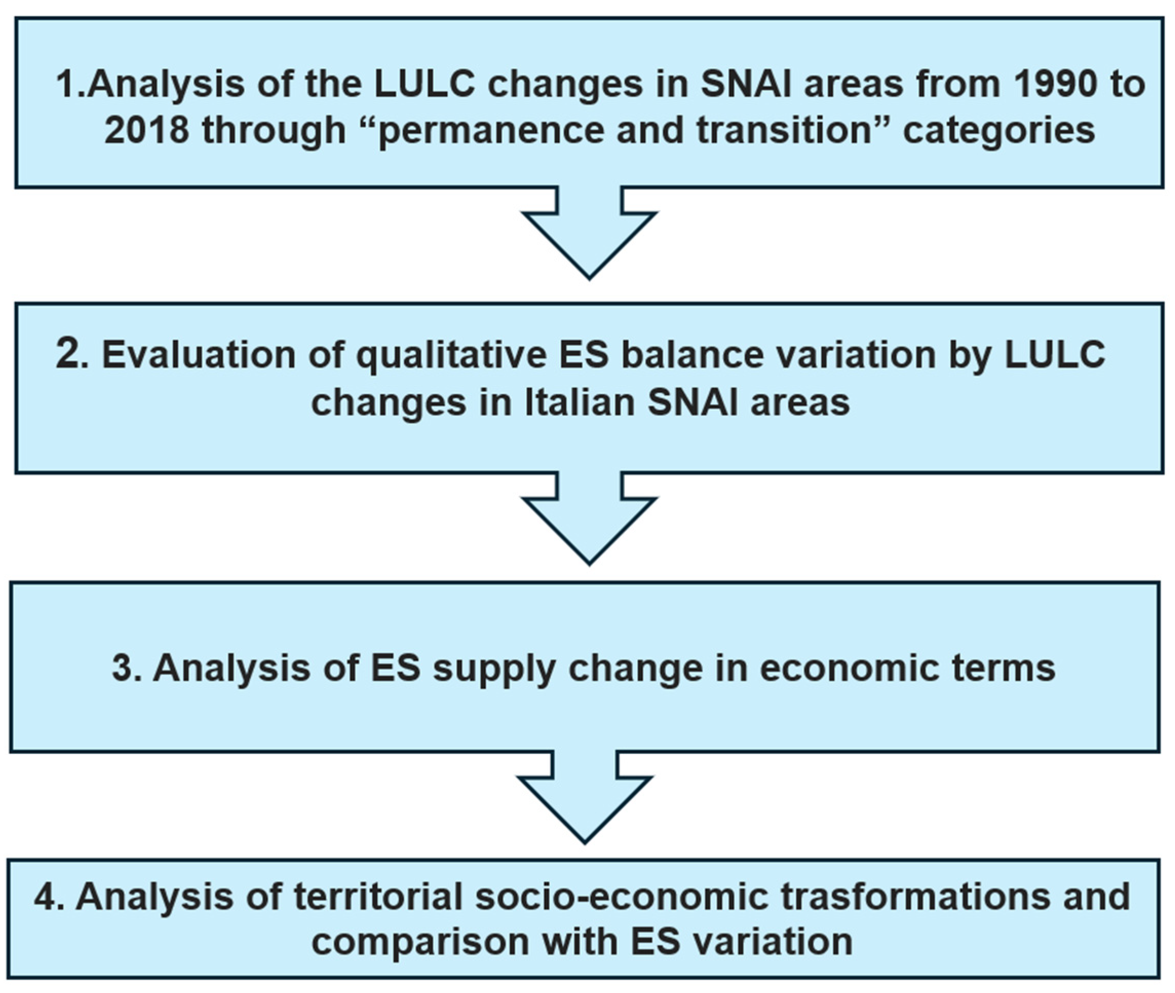
2.2. Analysis of the LULC Changes in SNAI Areas from 1990 to 2018 through Permanence and Transition Categories (Step 1)
2.3. Evaluation of ES Balance Variation by LULC Changes in Italian SNAI Areas (Step 2)
2.4. Economic Evaluation of the ES Supply in SNAI Areas (Step 3)
2.5. Analysis of Territorial Socio-Economic Transformations (Step 4)
3. Results
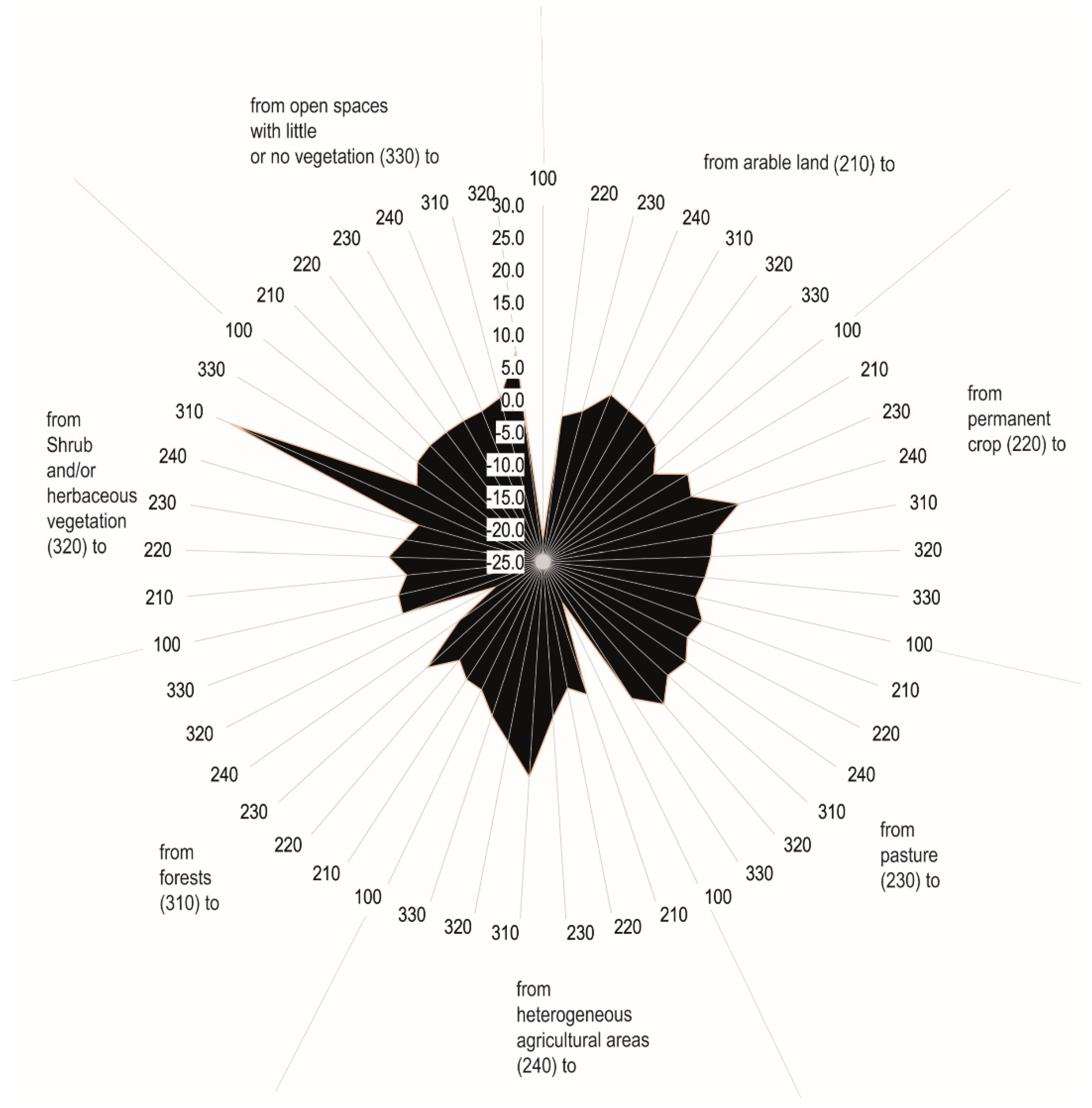
3.1. Main LULC Changes in SNAI Areas
3.2. Qualitative ES Balance Potential Variation
3.3. Economic Evaluation of the ES Supply
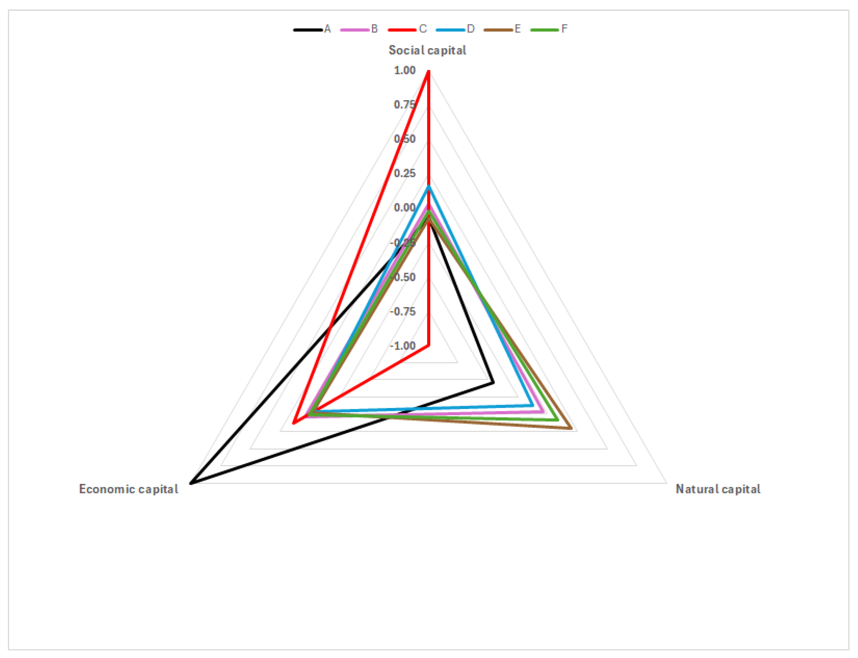
3.4. Analysis of Socio-Economic Transformations and Comparison with the Variation in the ES
4. Discussion
5. Conclusions
Author Contributions
Funding
Data Availability Statement
Conflicts of Interest
Appendix A


| A | 28,857 | B | 8746 | C | 84,605 | |||
| km2 | % | km2 | % | km2 | % | |||
| Perm (210210) | 9838 | 34 | Perm (210210) | 3114 | 36 | Perm (210210) | 29,016 | 34 |
| Perm (240240) | 4275 | 15 | Perm (310310) | 1599 | 18 | Perm (310310) | 15,622 | 18 |
| Perm (100100) | 3615 | 13 | Perm (240240) | 1183 | 14 | Perm (240240) | 11,662 | 14 |
| Perm (310310) | 3164 | 11 | Perm (220220) | 718 | 8 | Perm (220220) | 5954 | 7 |
| Perm (220220) | 2250 | 8 | Perm (100100) | 518 | 6 | Perm (100100) | 5340 | 6 |
| Perm (320320) | 1212 | 4 | Perm (500500) | 227 | 3 | Perm (320320) | 4064 | 5 |
| Perm (500500) | 552 | 2 | Perm (320320) | 226 | 3 | Etcs (210240) | 1200 | 1 |
| Int (240210) | 532 | 2 | Urb (240210) | 223 | 3 | Int (240210) | 1165 | 1 |
| Etcs (210240) | 438 | 2 | Etcs (210240) | 89 | 1 | Perm (330330) | 1099 | 1 |
| Urb (210100) | 408 | 1 | Int (240220) | 86 | 1 | Perm (500500) | 956 | 1 |
| Urb (240100) | 272 | 1 | Etcs (220240) | 76 | 1 | Urb (210100) | 886 | 1 |
| Etcs (220240) | 232 | 1 | Urb (210100) | 74 | 1 | Int (240220) | 810 | 1 |
| Int (240220) | 211 | 1 | Int (210220) | 68 | 1 | Etcs (220240) | 725 | 1 |
| Perm (320310) | 153 | 1 | Perm (330330) | 54 | 1 | Perm (230230) | 709 | 1 |
| Urb (240100) | 46 | 1 | Urb (240100) | 580 | 1 | |||
| Perm (320310) | 506 | 1 | ||||||
| Int (210220) | 492 | 1 | ||||||
| D | 87,705 | E | 72,397 | F | 19,296 | |||
| km2 | % | km2 | % | km2 | % | |||
| Perm (310310) | 25,010 | 29 | Perm (310310) | 23,292 | 32 | Perm (310310) | 5325 | 28 |
| Perm (210210) | 19,592 | 22 | Perm (210210) | 12,468 | 17 | Perm (320320) | 4761 | 25 |
| Perm (240240) | 11,121 | 13 | Perm (320320) | 10,317 | 14 | Perm (210210) | 2230 | 12 |
| Perm (320320) | 7854 | 9 | Perm (240240) | 7448 | 10 | Perm (240240) | 1797 | 9 |
| Perm (220220) | 5555 | 6 | Perm (330330) | 3361 | 5 | Perm (330330) | 1249 | 6 |
| Perm (330330) | 2605 | 3 | Perm (220220) | 2990 | 4 | Perm (320310) | 508 | 3 |
| Perm (100100) | 2099 | 2 | Perm (320310) | 1340 | 2 | Perm (220220) | 468 | 2 |
| Perm (500500) | 1239 | 1 | Perm (230230) | 1031 | 1 | Perm (310320) | 297 | 2 |
| Int (240210) | 1203 | 1 | Int (240210) | 917 | 1 | For Ext (240320) | 284 | 1 |
| Perm (320310) | 1145 | 1 | Perm (100100) | 895 | 1 | Perm (330320) | 231 | 1 |
| Etcs (210240) | 993 | 1 | Etcs (320240) | 818 | 1 | Etcs (320240) | 216 | 1 |
| Etcs (220240) | 988 | 1 | Perm (330320) | 758 | 1 | Int (240210) | 204 | 1 |
| Perm (230230) | 892 | 1 | Perm (310320) | 755 | 1 | Perm (100100) | 198 | 1 |
| Perm (330320) | 803 | 1 | Etcs (210240) | 583 | 1 | Int (320210) | 163 | 1 |
| Int (240220) | 669 | 1 | Perm (500500) | 564 | 1 | Etcs (210240) | 128 | 1 |
| Perm (310320) | 651 | 1 | Etcs (220240) | 557 | 1 | Perm (230230) | 123 | 1 |
| Etcs (320240) | 628 | 1 | Int (320210) | 488 | 1 | Etcs (220240) | 116 | 1 |
| Int (210220) | 554 | 1 | For Ext (240320) | 443 | 1 | Perm (500500) | 98 | 1 |
| Transition and Permanence | Change | Global Climate Regulation | Air Quality Regulation | Water Flow Regulation | Water Purifcation | Erosion Regulation | Natural Hazard Regulation | Crops | Fodder | Timber | Wild Food and Resources | Sum (0–5) |
|---|---|---|---|---|---|---|---|---|---|---|---|---|
| Urb | 210100 | −2 | −5 | −4 | −4 | 3 | −3 | −8 | −6 | −3 | −5 | −3 |
| Int | 210220 | 1 | 0 | 0 | −2 | 2 | −2 | −1 | −5 | 1 | −1 | 0 |
| Perm | 210230 | 0 | −1 | 0 | −2 | 3 | 0 | −5 | −5 | −1 | 1 | −1 |
| Etcs | 210240 | 2 | 0 | 1 | −1 | 4 | 0 | −2 | −3 | 1 | 1 | 0 |
| For Ext | 210310 | 6 | 5 | 3 | 5 | 8 | 5 | −5 | −4 | 5 | 4 | 2 |
| For Ext | 210320 | 4 | 1 | 1 | 2 | 6 | 2 | −5 | −3 | 1 | 2 | 1 |
| For Ext | 210330 | 1 | 0 | 1 | 1 | 4 | 2 | −5 | −5 | 0 | −1 | 0 |
| Urb | 220100 | −4 | −5 | −5 | −2 | 1 | −2 | −7 | −2 | −4 | −4 | −2 |
| Agr Ext | 220210 | −1 | 0 | 0 | 2 | −2 | 2 | 1 | 5 | −1 | 1 | 0 |
| Agr Ext | 220230 | −1 | −1 | 0 | 0 | 1 | 2 | −4 | 0 | −2 | 2 | 0 |
| Etcs | 220240 | 0 | 0 | 0 | 1 | 1 | 2 | 0 | 2 | −1 | 1 | 1 |
| For Ext | 220310 | 5 | 5 | 3 | 7 | 6 | 7 | −4 | 1 | 4 | 5 | 3 |
| For Ext | 220320 | 3 | 0 | 1 | 4 | 3 | 4 | −4 | 1 | 0 | 3 | 1 |
| For Ext | 220330 | 0 | 0 | 1 | 3 | 2 | 4 | −4 | 0 | −1 | 0 | 0 |
| Urb | 230100 | −2 | −4 | −4 | −2 | 0 | −3 | −3 | −2 | −2 | −6 | −2 |
| Int | 230210 | 0 | 1 | 0 | 2 | −3 | 0 | 5 | 5 | 1 | −1 | 1 |
| Int | 230220 | 1 | 1 | 0 | 0 | −1 | −2 | 4 | 0 | 2 | −2 | 0 |
| Etcs | 230240 | 1 | 1 | 0 | 1 | 1 | 0 | 3 | 2 | 2 | −1 | 1 |
| For Ext | 230310 | 6 | 6 | 3 | 7 | 5 | 5 | 0 | 1 | 6 | 3 | 3 |
| For Ext | 230320 | 4 | 2 | 1 | 4 | 3 | 2 | 0 | 1 | 2 | 1 | 1 |
| For Ext | 230330 | 1 | 1 | 1 | 3 | 1 | 2 | 0 | 0 | 1 | −2 | 1 |
| Urb | 240100 | −4 | −5 | −5 | −3 | 0 | −4 | −6 | −4 | −4 | −5 | −3 |
| Int | 240210 | −2 | 0 | −1 | 1 | −4 | 0 | 2 | 3 | −1 | −1 | 0 |
| Int | 240220 | 0 | 0 | 0 | −1 | −1 | −2 | 0 | −2 | 1 | −1 | −1 |
| Int | 240230 | −1 | −1 | 0 | −1 | −1 | 0 | −3 | −2 | −2 | 1 | −1 |
| For Ext | 240310 | 5 | 5 | 3 | 6 | 4 | 5 | −3 | −1 | 4 | 4 | 2 |
| For Ext | 240320 | 3 | 0 | 1 | 3 | 2 | 2 | −3 | −1 | 0 | 1 | 1 |
| For Ext | 240330 | 0 | 0 | 0 | 2 | 1 | 2 | −3 | −2 | −1 | −1 | 0 |
| Urb | 310100 | −8 | −10 | −7 | −9 | −5 | −8 | −3 | −3 | −8 | −9 | −5 |
| Int | 310210 | −6 | −5 | −3 | −5 | −8 | −5 | 5 | 4 | −5 | −4 | −2 |
| Int | 310220 | −5 | −5 | −3 | −7 | −6 | −7 | 4 | −1 | −4 | −5 | −3 |
| Int | 310230 | −6 | −6 | −3 | −7 | −5 | −5 | 0 | −1 | −6 | −3 | −3 |
| Etcs | 310240 | −5 | −5 | −3 | −6 | −4 | −5 | 3 | 1 | −4 | −4 | −2 |
| Perm | 310320 | −2 | −4 | −2 | −3 | −2 | −3 | 0 | 0 | −4 | −2 | −2 |
| Perm | 310330 | −5 | −5 | −2 | −4 | −4 | −3 | 0 | −1 | −5 | −5 | −2 |
| Urb | 320100 | −7 | −5 | −5 | −6 | −3 | −5 | −3 | −3 | −4 | −6 | −3 |
| Int | 320210 | −4 | −1 | −1 | −2 | −6 | −2 | 5 | 3 | −1 | −2 | −1 |
| Int | 320220 | −3 | 0 | −1 | −4 | −3 | −4 | 4 | −1 | 0 | −3 | −1 |
| Int | 320230 | −4 | −2 | −1 | −4 | −3 | −2 | 0 | −1 | −2 | −1 | −1 |
| Etcs | 320240 | −3 | 0 | −1 | −3 | −2 | −2 | 3 | 1 | 0 | −1 | −1 |
| Perm | 320310 | 2 | 4 | 2 | 3 | 2 | 3 | 0 | 0 | 4 | 2 | 2 |
| Perm | 320330 | −3 | −1 | 0 | −1 | −1 | 0 | 0 | −1 | −1 | −2 | −1 |
| Urb | 330100 | −3 | −5 | −5 | −5 | −1 | −5 | −3 | −2 | −3 | −4 | −3 |
| Int | 330210 | −1 | 0 | −1 | −1 | −4 | −2 | 5 | 5 | 0 | 1 | 0 |
| Int | 330220 | 0 | 0 | −1 | −3 | −2 | −4 | 4 | 0 | 1 | 0 | 0 |
| Int | 330230 | −1 | −1 | −1 | −3 | −1 | −2 | 0 | 0 | −1 | 2 | −1 |
| Etcs | 330240 | 0 | 0 | 0 | −2 | −1 | −2 | 3 | 2 | 1 | 1 | 0 |
| Perm | 330310 | 5 | 5 | 2 | 4 | 4 | 3 | 0 | 1 | 5 | 5 | 2 |
| Perm | 330320 | 3 | 1 | 0 | 1 | 1 | 0 | 0 | 1 | 1 | 2 | 1 |
| Perm Macro | − | 0 | 0 | 0 | 0 | 0 | 0 | 0 | 0 | 0 | 0 | 0 |
| Other | − | 1 | 1 | 1 | 1 | 0 | 1 | 1 | 1 | 1 | 1 | 0 |
| tot | −3 | −4 | −5 | −4 | 0 | −4 | −4 | −3 | −2 | −5 | −2 |
| Transition and Permanence | Change | km2 | Global Climate Regulation | Air Quality Regulation | Water Flow Regulation | Water Purification | Erosion Regulation | Natural Hazard Regulation | Crops | Fodder | Timber | Wild Food and Resources | Sum |
|---|---|---|---|---|---|---|---|---|---|---|---|---|---|
| Urb | 210100 | 1725 | −1.3 | −2.7 | −2.5 | −2.2 | 1.8 | −1.8 | −4.6 | −3.7 | −1.8 | −2.7 | −21.5 |
| Int | 210220 | 1496 | 0.6 | 0.1 | 0.2 | −0.8 | 1.1 | −0.8 | −0.5 | −2.4 | 0.5 | −0.5 | −2.4 |
| Perm | 210230 | 299 | 0.0 | −0.1 | 0.0 | −0.2 | 0.3 | 0.0 | −0.5 | −0.5 | −0.1 | 0.1 | −0.9 |
| Etcs | 210240 | 3430 | 1.8 | 0.5 | 0.7 | −1.0 | 4.0 | 0.5 | −1.7 | −3.1 | 0.6 | 0.6 | 2.8 |
| For Ext | 210310 | 173 | 0.3 | 0.3 | 0.2 | 0.3 | 0.5 | 0.3 | −0.3 | −0.2 | 0.3 | 0.2 | 1.9 |
| For Ext | 210320 | 398 | 0.6 | 0.1 | 0.2 | 0.3 | 0.7 | 0.3 | −0.7 | −0.5 | 0.1 | 0.2 | 1.3 |
| For Ext | 210330 | 46 | 0.0 | − | 0.0 | 0.0 | 0.1 | 0.0 | −0.1 | −0.1 | − | −0.0 | −0.0 |
| Urb | 220100 | 294 | −0.3 | −0.5 | −0.5 | −0.2 | 0.1 | −0.2 | −0.7 | −0.2 | −0.4 | −0.4 | −3.2 |
| Agr Ext | 220210 | 695 | −0.3 | −0.1 | −0.1 | 0.4 | −0.5 | 0.4 | 0.2 | 1.1 | −0.2 | 0.2 | 1.1 |
| Agr Ext | 220230 | 20 | −0.0 | −0.0 | −0.0 | −0.0 | 0.0 | 0.0 | −0.0 | −0.0 | −0.0 | 0.0 | −0.0 |
| Etcs | 220240 | 2694 | 0.2 | 0.2 | 0.2 | 0.6 | 1.2 | 1.7 | −0.4 | 1.9 | −0.5 | 1.3 | 6.5 |
| For Ext | 220310 | 126 | 0.2 | 0.2 | 0.1 | 0.3 | 0.2 | 0.3 | −0.2 | 0.0 | 0.2 | 0.2 | 1.6 |
| For Ext | 220320 | 174 | 0.2 | 0.0 | 0.0 | 0.2 | 0.2 | 0.2 | −0.2 | 0.1 | −0.0 | 0.1 | 0.8 |
| For Ext | 220330 | 33 | −0.0 | −0.0 | 0.0 | 0.0 | 0.0 | 0.0 | −0.0 | −0.0 | −0.0 | 0.0 | 0.0 |
| Urb | 230100 | 89 | −0.1 | −0.1 | −0.1 | −0.1 | 0.0 | −0.1 | −0.1 | −0.0 | −0.1 | −0.2 | −0.8 |
| Int | 230210 | 357 | −0.0 | 0.1 | −0.0 | 0.2 | −0.4 | −0.0 | 0.6 | 0.6 | 0.1 | −0.1 | 1.1 |
| Int | 230220 | 47 | 0.0 | 0.0 | 0.0 | 0.0 | −0.0 | −0.0 | 0.1 | 0.0 | 0.0 | −0.0 | 0.1 |
| Etcs | 230240 | 463 | 0.2 | 0.2 | 0.1 | 0.1 | 0.1 | 0.1 | 0.5 | 0.3 | 0.2 | −0.1 | 1.8 |
| For Ext | 230310 | 67 | 0.1 | 0.1 | 0.1 | 0.2 | 0.1 | 0.1 | − | 0.0 | 0.1 | 0.1 | 0.9 |
| For Ext | 230320 | 587 | 0.8 | 0.3 | 0.2 | 0.8 | 0.5 | 0.4 | − | 0.3 | 0.4 | 0.1 | 3.8 |
| For Ext | 230330 | 10 | 0.0 | 0.0 | 0.0 | 0.0 | 0.0 | 0.0 | − | − | 0.0 | −0.0 | 0.0 |
| Urb | 240100 | 1357 | −1.7 | −2.3 | −2.2 | −1.4 | −0.2 | −1.6 | −2.9 | −1.7 | −1.7 | −2.4 | −18.0 |
| Int | 240210 | 4245 | −2.2 | −0.7 | −0.9 | 1.2 | −5.0 | −0.6 | 2.1 | 3.9 | −0.8 | −0.7 | −3.5 |
| Int | 240220 | 2158 | −0.2 | −0.2 | −0.2 | −0.5 | −1.0 | −1.4 | 0.3 | −1.5 | 0.4 | −1.0 | −5.2 |
| Int | 240230 | 259 | −0.1 | −0.1 | −0.0 | −0.1 | −0.0 | −0.0 | −0.3 | −0.2 | −0.1 | 0.0 | −1.0 |
| For Ext | 240310 | 819 | 1.2 | 1.2 | 0.7 | 1.6 | 1.2 | 1.3 | −0.9 | −0.3 | 1.2 | 1.0 | 8.2 |
| For Ext | 240320 | 1320 | 1.2 | 0.0 | 0.3 | 1.3 | 0.9 | 0.7 | −1.5 | −0.3 | 0.1 | 0.5 | 3.2 |
| For Ext | 240330 | 75 | −0.0 | −0.0 | 0.0 | 0.0 | 0.0 | 0.0 | −0.1 | −0.1 | −0.0 | −0.0 | −0.1 |
| Urb | 310100 | 137 | −0.4 | −0.4 | −0.3 | −0.4 | −0.2 | −0.4 | −0.1 | −0.1 | −0.4 | −0.4 | −3.2 |
| Int | 310210 | 315 | −0.6 | −0.5 | −0.3 | −0.5 | −0.8 | −0.5 | 0.5 | 0.4 | −0.5 | −0.4 | −3.4 |
| Int | 310220 | 415 | −0.7 | −0.7 | −0.4 | −0.9 | −0.8 | −0.9 | 0.5 | −0.1 | −0.5 | −0.7 | −5.1 |
| Int | 310230 | 59 | −0.1 | −0.1 | −0.1 | −0.1 | −0.1 | −0.1 | − | −0.0 | −0.1 | −0.1 | −0.8 |
| Etcs | 310240 | 928 | −1.4 | −1.4 | −0.8 | −1.9 | −1.4 | −1.4 | 1.1 | 0.3 | −1.4 | −1.1 | −9.3 |
| Perm | 310320 | 2219 | −1.3 | −3.3 | −1.4 | −2.3 | −1.7 | −2.2 | − | 0.3 | −3.1 | −1.7 | −16.7 |
| Perm | 310330 | 177 | −0.3 | −0.3 | −0.1 | −0.2 | −0.2 | −0.2 | − | −0.1 | −0.3 | −0.3 | −1.9 |
| Urb | 320100 | 136 | −0.3 | −0.2 | −0.2 | −0.3 | −0.1 | −0.2 | −0.1 | −0.1 | −0.2 | −0.3 | −2.1 |
| Int | 320210 | 1190 | −1.7 | −0.2 | −0.5 | −0.8 | −2.2 | −0.8 | 2.0 | 1.4 | −0.3 | −0.7 | −3.9 |
| Int | 320220 | 243 | −0.2 | −0.0 | −0.1 | −0.3 | −0.3 | −0.3 | 0.3 | −0.1 | 0.0 | −0.2 | −1.2 |
| Int | 320230 | 543 | −0.8 | −0.3 | −0.2 | −0.7 | −0.5 | −0.4 | − | −0.3 | −0.3 | −0.1 | −3.5 |
| Etcs | 320240 | 2037 | −1.9 | −0.1 | −0.4 | −2.0 | −1.4 | −1.1 | 2.4 | 0.5 | −0.2 | −0.8 | −5.0 |
| Perm | 320310 | 3692 | 2.2 | 5.4 | 2.4 | 3.8 | 2.9 | 3.6 | − | −0.5 | 5.1 | 2.9 | 27.8 |
| Perm | 320330 | 646 | −0.7 | −0.1 | −0.1 | −0.2 | −0.3 | 0.0 | − | −0.3 | −0.2 | −0.5 | −2.3 |
| Urb | 330100 | 18 | −0.0 | −0.0 | −0.0 | −0.0 | −0.0 | −0.0 | −0.0 | −0.0 | −0.0 | −0.0 | −0.2 |
| Int | 330210 | 60 | −0.0 | − | −0.0 | −0.0 | −0.1 | −0.0 | 0.1 | 0.1 | − | 0.0 | 0.0 |
| Int | 330220 | 17 | 0.0 | 0.0 | −0.0 | −0.0 | −0.0 | −0.0 | 0.0 | 0.0 | 0.0 | −0.0 | −0.0 |
| Int | 330230 | 8 | −0.0 | −0.0 | −0.0 | −0.0 | −0.0 | −0.0 | − | − | −0.0 | 0.0 | −0.0 |
| Etcs | 330240 | 99 | 0.0 | 0.0 | −0.0 | −0.1 | −0.0 | −0.1 | 0.1 | 0.1 | 0.0 | 0.0 | 0.1 |
| Perm | 330310 | 108 | 0.2 | 0.2 | 0.1 | 0.1 | 0.1 | 0.1 | − | 0.0 | 0.2 | 0.2 | 1.2 |
| Perm | 330320 | 2200 | 2.3 | 0.4 | 0.3 | 0.7 | 1.0 | −0.1 | − | 1.0 | 0.6 | 1.6 | 7.7 |
| Perm Macro | - | 261,823 | − | − | − | − | − | − | − | − | − | − | −0.0 |
| Other | - | 1080 | 0.9 | 1.2 | 1.2 | 0.9 | −0.0 | 0.9 | 1.3 | 0.8 | 0.8 | 1.2 | 9.0 |
| tot | 301,605 | −3.5 | −3.7 | −4.5 | −4.1 | −0.2 | −4.3 | −3.8 | −3.2 | −2.2 | −4.7 | −34.1 |
| A | −9.3 | B | −1.4 | C | −21.7 | D | −3.1 | E | 0.1 | F | 1.3 |
|---|---|---|---|---|---|---|---|---|---|---|---|
| 210100 | −5.1 | 210100 | −0.9 | 210100 | −11.0 | 310320 | −4.9 | 310320 | −5.7 | 310320 | −2.2 |
| 240100 | −3.6 | 240100 | −0.6 | 240100 | −7.7 | 240100 | −3.7 | 310240 | −2.6 | 310240 | −0.5 |
| 310320 | −0.7 | 310320 | −3.0 | 210100 | −3.2 | 320240 | −2.0 | 320210 | −0.5 | ||
| 220100 | −0.6 | 310220 | −2.6 | 310240 | −2.9 | 320230 | −1.9 | 320240 | −0.5 | ||
| 310100 | −0.6 | 310240 | −2.5 | 240220 | −1.6 | 240100 | −1.9 | 240100 | −0.5 | ||
| 240220 | −0.5 | 240220 | −2.0 | 310220 | −1.6 | 320210 | −1.6 | 240310 | 0.6 | ||
| 310240 | −0.5 | 310210 | −1.5 | 320240 | −1.5 | 210100 | −1.1 | 240320 | 0.7 | ||
| 320100 | −0.5 | 220100 | −1.3 | 320210 | −1.1 | 320330 | −0.9 | 330320 | 0.8 | ||
| 240310 | 0.5 | 310100 | −1.0 | 240210 | −1.0 | 240210 | −0.8 | 320310 | 3.8 | ||
| 220240 | 0.6 | 240210 | −1.0 | 320230 | −0.9 | 240220 | −0.7 | ||||
| 320310 | 1.1 | 210220 | −0.8 | 210220 | −0.9 | 310330 | −0.5 | ||||
| 320100 | −0.6 | 310100 | −0.9 | 310210 | −0.5 | ||||||
| 320240 | −0.6 | 310210 | −0.9 | 310100 | −0.5 | ||||||
| 310330 | −0.5 | 220100 | −0.8 | 210240 | 0.5 | ||||||
| 230320 | 0.9 | 320330 | −0.5 | 230240 | 0.6 | ||||||
| 210240 | 1.0 | 330310 | 0.5 | 230320 | 0.7 | ||||||
| 330320 | 1.2 | 210310 | 0.5 | 240320 | 1.1 | ||||||
| 220240 | 1.8 | 230240 | 0.6 | 220240 | 1.3 | ||||||
| 240310 | 1.8 | 240320 | 0.8 | 240310 | 2.6 | ||||||
| 320310 | 3.8 | 210240 | 0.8 | 330320 | 2.7 | ||||||
| 230320 | 1.5 | 320310 | 10.1 | ||||||||
| 220240 | 2.4 | ||||||||||
| 240310 | 2.5 | ||||||||||
| 330320 | 2.8 | ||||||||||
| 320310 | 8.6 |
References
- Accordo di Partenariato 2014–2020, Strategia nazionale per le Aree interne: Definizione, obiettivi, strumenti e governance. Aedon Riv. di Arti e Dirit. Line 2018, 3, 1–70. [CrossRef]
- Vatitsi, K.; Ioannidou, N.; Mirli, A.; Siachalou, S.; Kagalou, I.; Latinopoulos, D.; Mallinis, G. LULC Change Effects on Environmental Quality and Ecosystem Services Using EO Data in Two Rural River Basins in Thrace, Greece. Land 2023, 12, 1140. [Google Scholar] [CrossRef]
- Egarter Vigl, L.; Tasser, E.; Schirpke, U.; Tappeiner, U. Using Land Use/Land Cover Trajectories to Uncover Ecosystem Service Patterns across the Alps. Reg. Environ. Chang. 2017, 17, 2237–2250. [Google Scholar] [CrossRef]
- Fang, Z.; Ding, T.; Chen, J.; Xue, S.; Zhou, Q.; Wang, Y.; Wang, Y.; Huang, Z.; Yang, S. Impacts of Land Use/Land Cover Changes on Ecosystem Services in Ecologically Fragile Regions. Sci. Total Environ. 2022, 831, 154967. [Google Scholar] [CrossRef]
- Kuang, W.; Du, G.; Lu, D.; Dou, Y.; Li, X.; Zhang, S.; Chi, W.; Dong, J.; Chen, G.; Yin, Z.; et al. Global Observation of Urban Expansion and Land-Cover Dynamics Using Satellite Big-Data. Sci. Bull. 2021, 66, 297–300. [Google Scholar] [CrossRef]
- Buytaert, W.; Zulkafli, Z.; Grainger, S.; Acosta, L.; Alemie, T.C.; Bastiaensen, J.; De Bièvre, B.; Bhusal, J.; Clark, J.; Dewulf, A.; et al. Citizen Science in Hydrology and Water Resources: Opportunities for Knowledge Generation, Ecosystem Service Management, and Sustainable Development. Front. Earth Sci. 2014, 2, 26. [Google Scholar] [CrossRef]
- Geijzendorffer, I.R.; Roche, P.K. The Relevant Scales of Ecosystem Services Demand. Ecosyst. Serv. 2014, 10, 49–51. [Google Scholar] [CrossRef]
- Meisch, C.; Schirpke, U.; Huber, L.; Rüdisser, J.; Tappeiner, U. Assessing Freshwater Provision and Consumption in the Alpine Space Applying the Ecosystem Service Concept. Sustainability 2019, 11, 1131. [Google Scholar] [CrossRef]
- Zhang, Z.; Liu, Y.; Wang, Y.; Liu, Y.; Zhang, Y.; Zhang, Y. What Factors Affect the Synergy and Tradeoff between Ecosystem Services, and How, from a Geospatial Perspective? J. Clean. Prod. 2020, 257, 120454. [Google Scholar] [CrossRef]
- Zhang, L.; Huang, Q.; He, C.; Yue, H.; Zhao, Q. Assessing the Dynamics of Sustainability for Social-Ecological Systems Based on the Adaptive Cycle Framework: A Case Study in the Beijing-Tianjin-Hebei Urban Agglomeration. Sustain. Cities Soc. 2021, 70, 102899. [Google Scholar] [CrossRef]
- Wei, H.; Fan, W.; Wang, X.; Lu, N.; Dong, X.; Zhao, Y.; Ya, X.; Zhao, Y. Integrating Supply and Social Demand in Ecosystem Services Assessment: A Review. Ecosyst. Serv. 2017, 25, 15–27. [Google Scholar] [CrossRef]
- Schirpke, U.; Tasser, E.; Borsky, S.; Braun, M.; Eitzinger, J.; Gaube, V.; Getzner, M.; Glatzel, S.; Gschwantner, T.; Kirchner, M.; et al. Past and Future Impacts of Land-Use Changes on Ecosystem Services in Austria. J. Environ. Manag. 2023, 345, 118728. [Google Scholar] [CrossRef]
- Oppio, A. Migrants and Italian Inner Areas for an Anti-Fragility Strategy. Valori Valutazioni 2021, 2021, 93–102. [Google Scholar] [CrossRef]
- Dax, T.; Schroll, K.; Machold, I.; Derszniak-Noirjean, M.; Schuh, B.; Gaupp-Berghausen, M. Land Abandonment in Mountain Areas of the EU: An Inevitable Side Effect of Farming Modernization and Neglected Threat to Sustainable Land Use. Land 2021, 10, 591. [Google Scholar] [CrossRef]
- Marino, D.; Palmieri, M.; Marucci, A.; Pili, S. Long-Term Land Cover Changes and Ecosystem Services Variation: Have the Anthropogenic Transformations Degraded Human Well-Being in Italy? Ital. Rev. Agric. Econ. 2022, 77, 7–23. [Google Scholar] [CrossRef]
- Esengulova, N.; Balena, P.; De Lucia, C.; Lopolito, A.; Pazienza, P. Key Drivers of Land Use Changes in the Rural Area of Gargano (South Italy) and Their Implications for the Local Sustainable Development. Land 2024, 13, 166. [Google Scholar] [CrossRef]
- McPhearson, T.; Cook, E.M.; Berbés-Blázquez, M.; Cheng, C.; Grimm, N.B.; Andersson, E.; Barbosa, O.; Chandler, D.G.; Chang, H.; Chester, M.V.; et al. A Social-Ecological-Technological Systems Framework for Urban Ecosystem Services. One Earth 2022, 5, 505–518. [Google Scholar] [CrossRef]
- Costanza, R.; de Groot, R.; Sutton, P.; van der Ploeg, S.; Anderson, S.J.; Kubiszewski, I.; Farber, S.; Turner, R.K. Changes in the Global Value of Ecosystem Services. Glob. Environ. Chang. 2014, 26, 152–158. [Google Scholar] [CrossRef]
- de Groot, R.; Brander, L.; van der Ploeg, S.; Costanza, R.; Bernard, F.; Braat, L.; Christie, M.; Crossman, N.; Ghermandi, A.; Hein, L.; et al. Global Estimates of the Value of Ecosystems and Their Services in Monetary Units. Ecosyst. Serv. 2012, 1, 50–61. [Google Scholar] [CrossRef]
- Blumstein, M.; Thompson, J.R. Land-Use Impacts on the Quantity and Configuration of Ecosystem Service Provisioning in Massachusetts, USA. J. Appl. Ecol. 2015, 52, 1009–1019. [Google Scholar] [CrossRef]
- Schirpke, U.; Tscholl, S.; Tasser, E. Spatio-Temporal Changes in Ecosystem Service Values: Effects of Land-Use Changes from Past to Future (1860–2100). J. Environ. Manag. 2020, 272, 111068. [Google Scholar] [CrossRef] [PubMed]
- García-Nieto, A.P.; Geijzendorffer, I.R.; Baró, F.; Roche, P.K.; Bondeau, A.; Cramer, W. Impacts of Urbanization around Mediterranean Cities: Changes in Ecosystem Service Supply. Ecol. Indic. 2018, 91, 589–606. [Google Scholar] [CrossRef]
- Gomes, E.; Inácio, M.; Bogdzevič, K.; Kalinauskas, M.; Karnauskaitė, D.; Pereira, P. Future Land-Use Changes and Its Impacts on Terrestrial Ecosystem Services: A Review. Sci. Total. Environ. 2021, 781, 146716. [Google Scholar] [CrossRef] [PubMed]
- Marucci, A.; Marino, D.; Palmieri, M.; Pili, S. The Role of Agroforestry Areas in the Potential Provision of Ecosystem Services: The Case of the Molise Region. L’Ital. For. Mont. 2022, 77, 153–163. [Google Scholar] [CrossRef]
- Han, Z.; Song, W.; Deng, X.; Xu, X. Trade-Offs and Synergies in Ecosystem Service within the Three-Rivers Headwater Region, China. Water 2017, 9, 588. [Google Scholar] [CrossRef]
- Mendoza-González, G.; Martínez, M.L.; Lithgow, D.; Pérez-Maqueo, O.; Simonin, P. Land Use Change and Its Effects on the Value of Ecosystem Services along the Coast of the Gulf of Mexico. Ecol. Econ. 2012, 82, 23–32. [Google Scholar] [CrossRef]
- Burkhard, B.; Santos-Martin, F.; Nedkov, S.; Maes, J. An Operational Framework for Integrated Mapping and Assessment of Ecosystems and Their Services (MAES). One Ecosyst. 2018, 3, e22831. [Google Scholar] [CrossRef]
- Burkhard, B.; Kandziora, M.; Hou, Y.; Müller, F. Ecosystem Service Potentials, Flows and Demands-Concepts for Spatial Localisation, Indication and Quantification. Landsc. Online 2014, 34, 1–32. [Google Scholar] [CrossRef]
- Pandeya, B.; Buytaert, W.; Zulkafli, Z.; Karpouzoglou, T.; Mao, F.; Hannah, D.M. A Comparative Analysis of Ecosystem Services Valuation Approaches for Application at the Local Scale and in Data Scarce Regions. Ecosyst. Serv. 2016, 22, 250–259. [Google Scholar] [CrossRef]
- Schild, J.E.M.; Vermaat, J.E.; van Bodegom, P.M. Differential Effects of Valuation Method and Ecosystem Type on the Monetary Valuation of Dryland Ecosystem Services: A Quantitative Analysis. J. Arid Environ. 2018, 159, 11–21. [Google Scholar] [CrossRef]
- Marino, D.; Barone, A.; Marucci, A.; Pili, S.; Palmieri, M. Impact of Land Use Changes on Ecosystem Services Supply: A Meta Analysis of the Italian Context. Land 2023, 12, 2173. [Google Scholar] [CrossRef]
- Ecosystem Services Valuation Database. Available online: https://www.esvd.info/ (accessed on 8 August 2023).
- SINAnet Groupware. Available online: https://groupware.sinanet.isprambiente.it/uso-copertura-e-consumo-di-suolo/library/copertura-del-suolo/corine-land-cover (accessed on 25 March 2024).
- Istat Aree Interne. Available online: https://www.istat.it/notizia/la-geografia-delle-aree-interne-nel-2020-vasti-territori-tra-potenzialita-e-debolezze/ (accessed on 25 March 2024).
- Burkhard, B.; Kroll, F.; Müller, F.; Windhorst, W. Landscapes’ Capacities to Provide Ecosystem Services—A Concept for Land-Cover Based Assessments. Landsc. Online 2009, 15, 1–22. [Google Scholar] [CrossRef]
- Burkhard, B.; Kroll, F.; Nedkov, S.; Müller, F. Mapping Ecosystem Service Supply, Demand and Budgets. Ecol. Indic. 2012, 21, 17–29. [Google Scholar] [CrossRef]
- Jacobs, S.; Burkhard, B.; Van Daele, T.; Staes, J.; Schneiders, A. ‘The Matrix Reloaded’: A Review of Expert Knowledge Use for Mapping Ecosystem Services. Ecol. Model. 2015, 295, 21–30. [Google Scholar] [CrossRef]
- Bateman, I.J.; Harwood, A.R.; Mace, G.M.; Watson, R.T.; Abson, D.J.; Andrews, B.; Binner, A.; Crowe, A.; Day, B.H.; Dugdale, S.; et al. Bringing Ecosystem Services into Economic Decision-Making: Land Use in the United Kingdom. Science 2013, 341, 45–50. [Google Scholar] [CrossRef]
- Boutwell, J.L.; Westra, J.V. Benefit Transfer: A Review of Methodologies and Challenges. Resources 2013, 2, 517–527. [Google Scholar] [CrossRef]
- Richardson, L.; Loomis, J.; Kroeger, T.; Casey, F. The Role of Benefit Transfer in Ecosystem Service Valuation. Ecol. Econ. 2015, 115, 51–58. [Google Scholar] [CrossRef]
- ISTAT ASC. Available online: https://asc.istat.it/ASC/ (accessed on 1 June 2024).
- D’Andria, E.; Fiore, P. The RI.P.R.O.VA.RE. Project for the Regeneration of Inland Areas: A Focus on the Ufita Area in the Campania Region (Italy). Buildings 2023, 13, 336. [Google Scholar] [CrossRef]
- Tantillo, F. Una Strategia per Le Aree Interne. In Borgofuturo+: Un Progetto Locale per le Aree Interne; Quodlibet: Macerata, Italy, 2022; pp. 57–62. [Google Scholar] [CrossRef]
- Fenu, N.; Giaccaria, P. La Scommessa della SNAI. La Strategia Nazionale delle Aree Interne. 2023. Available online: https://www.documentigeografici.it/index.php/docugeo/article/view/476 (accessed on 1 June 2024).
- Lucia, C.; Annunziata, P. Spatial Analysis for Territorial Marginality Mapping. GIS-Based Application to the Case of Southern and Insular Italy. In Proceedings of the SUPTM 2022: 1st Conference on Future Challenges in Sustainable Urban Planning & Territorial Management, Online, 17–19 January 2022; pp. 1–4. [Google Scholar] [CrossRef]
- Pilogallo, A.; Scorza, F.; Murgante, B. Ecosystem Services-Based City Ranking in Italy: A Tool to Enhance Sustainable Thinking in Regeneration Strategies. Land 2024, 13, 891. [Google Scholar] [CrossRef]
- Wang, Y.; Rao, Y.; Zhu, H. Analyzing the Land Use and Cover Change Inside and Outside China’s Ecological Function Area. Land 2023, 12, 1447. [Google Scholar] [CrossRef]
- Shen, J.; Li, S.; Liu, L.; Liang, Z.; Wang, Y.; Wang, H.; Wu, S. Uncovering the Relationships between Ecosystem Services and Social-Ecological Drivers at Different Spatial Scales in the Beijing-Tianjin-Hebei Region. J. Clean. Prod. 2021, 290, 125193. [Google Scholar] [CrossRef]
- Luo, Y.; Yang, D.; O’Connor, P.; Wu, T.; Ma, W.; Xu, L.; Guo, R.; Lin, J. Dynamic Characteristics and Synergistic Effects of Ecosystem Services under Climate Change Scenarios on the Qinghai–Tibet Plateau. Sci. Rep. 2022, 12, 2540. [Google Scholar] [CrossRef] [PubMed]
- Marino, D.; Palmieri, M.; Marucci, A.; Tufano, M. Comparison between Demand and Supply of Some Ecosystem Services in National Parks: A Spatial Analysis Conducted Using Italian Case Studies. Conservation 2021, 1, 36–57. [Google Scholar] [CrossRef]
- Pearce, D.W.; Turner, R.K. Economics of Natural Resources and the Environment; Harvester Wheatsheaf: Birmingham, UK, 1990; ISBN 0 7450 0225 0. [Google Scholar]
- Marino, D.; Palmieri, M. Investing in nature: Working with public expenditure and private payments for a new governance model. In Reconnecting Natural and Cultural Capital: Contributions from Science and Policy; Paracchini, M.L., Zingari, P.C., Blasi, C., Eds.; European Commission, Joint Research Centre: Brussels, Belgium, 2018; ISBN 9789279599491. [Google Scholar]
- Putnam, R.D. Tuning in, turning out: The strange disappearance of social capital in America. Political Sci. Politics 1995, 27, 64–83. [Google Scholar]
- You, C.; Qu, H.; Wang, C.; Feng, C.C.; Guo, L. Trade-off and Synergistic of Ecosystem Services Supply and Demand Based on Socio-Ecological System (SES) in Typical Hilly Regions of South China. Ecol. Indic. 2024, 160, 111749. [Google Scholar] [CrossRef]
- Ekins, P. Identifying Critical Natural Capital Conclusions about Critical Natural Capital. Ecol. Econ. 2003, 44, 277–292. [Google Scholar] [CrossRef]
- Chaplin-Kramer, R.; Neugarten, R.A.; Sharp, R.P.; Collins, P.M.; Polasky, S.; Hole, D.; Schuster, R.; Strimas-Mackey, M.; Mulligan, M.; Brandon, C.; et al. Mapping the Planet’s Critical Natural Assets. Nat. Ecol. Evol. 2023, 7, 51–61. [Google Scholar] [CrossRef]
- Raudsepp-Hearne, C.; Peterson, G.D.; Bennett, E.M. Ecosystem Service Bundles for Analyzing Tradeoffs in Diverse Landscapes. Proc. Natl. Acad. Sci. USA 2010, 107, 5242–5247. [Google Scholar] [CrossRef] [PubMed]
- Rossitti, M.; Dell’ovo, M.; Oppio, A.; Torrieri, F. The Italian National Strategy for Inner Areas (Snai): A Critical Analysis of the Indicator Grid. Sustainability 2021, 13, 6927. [Google Scholar] [CrossRef]
- Porta, A.; Segre, G.; Arauzo-Carod, J.M. The Italian National Strategy for Inner Areas: First Insights from Regions’ Specialization in Cultural and Creative Industries. In Clusters in Times of Uncertainty; Edward Elgar Publishing: Cheltenham, UK, 2024; pp. 240–261. [Google Scholar] [CrossRef]
- Pettenella, D.; Romano, R. Le Foreste Delle Aree Interne: Potenzialità Di Sviluppo Dell’economia Locale e Di Offerta Di Beni Pubblici. Agriregionieuropa 2016, 12, 50–55. [Google Scholar]
- Obst, C.; Hein, L.; Edens, B. National Accounting and the Valuation of Ecosystem Assets and Their Services. Environ. Resour. Econ. 2016, 64, 1–23. [Google Scholar] [CrossRef]

| SNAI Description | SNAI Code | Urban Areas | Agricultural Areas | Wooded and Semi-Natural Areas | Wetlands and Water Bodies | Total | ||||
|---|---|---|---|---|---|---|---|---|---|---|
| km2 | % | km2 | % | km2 | % | km2 | % | km2 | ||
| Hubs | A | 4424 | 15% | 18,706 | 65% | 5135 | 18% | 592 | 2% | 28,857 |
| Intermediate hubs | B | 661 | 8% | 5782 | 66% | 2062 | 24% | 242 | 3% | 8746 |
| Belt | C | 7060 | 8% | 53,602 | 63% | 22,905 | 27% | 1037 | 1% | 84,605 |
| Intermediate | D | 2801 | 3% | 44,168 | 50% | 39,448 | 45% | 1288 | 1% | 87,705 |
| Peripheral | E | 1219 | 2% | 29,230 | 40% | 41,340 | 57% | 608 | 1% | 72,397 |
| Ultraperipheral | F | 279 | 1% | 5825 | 30% | 13,079 | 68% | 112 | 1% | 19,296 |
| Total | 16,444 | 5% | 157,313 | 52% | 123,969 | 41% | 3879 | 1% | 301,605 | |
| Macroclass Description | Macroclass Code | Global Climate Regulation | Air Quality Regulation | Water Flow Regulation | Water Purification | Erosion Regulation | Natural Hazard Regulation | Crops | Fodder | Timber | Wild Food and Resources |
|---|---|---|---|---|---|---|---|---|---|---|---|
| Urban areas | 100 | −3.3 | −4.7 | −4.4 | −4.1 | 0.1 | −4.2 | −3.0 | −1.6 | −3.2 | −3.8 |
| Arable lands | 210 | −1.1 | 0.0 | −0.1 | −0.2 | −3.0 | −1.0 | 5.0 | 4.9 | 0.0 | 1.0 |
| Permanent crops | 220 | 0.2 | 0.2 | 0.2 | −1.7 | −0.8 | −2.6 | 4.0 | 0.0 | 1.1 | 0.1 |
| Pastures | 230 | −1.0 | −1.0 | 0.0 | −2.0 | 0.0 | −1.0 | 0.0 | 0.0 | −1.0 | 2.0 |
| Heterogeneous agricultural areas | 240 | 0.5 | 0.5 | 0.5 | −1.1 | 0.6 | −0.6 | 3.5 | 2.1 | 0.5 | 1.5 |
| Forests | 310 | 5.0 | 5.0 | 3.0 | 5.0 | 5.0 | 4.0 | 0.0 | 1.0 | 5.0 | 5.0 |
| Shrub and/or herbaceous vegetation | 320 | 3.2 | 0.5 | 1.1 | 1.9 | 2.6 | 1.1 | 0.0 | 1.4 | 0.8 | 2.6 |
| Non and sparsely vegetated areas | 330 | 0.1 | 0.0 | 0.7 | 0.9 | 1.3 | 1.3 | 0.0 | 0.0 | 0.0 | 0.4 |
| Wetland and water bodies | 500 | 0.9 | 0.0 | 3.9 | 2.0 | 0.2 | 3.3 | 0.0 | 0.4 | 0.0 | 3.5 |
| LULC Permanence and Transition Categories | A | B | C | D | E | F |
|---|---|---|---|---|---|---|
| Agr. Extensification | 0.3% | 0.5% | 0.3% | 0.3% | 0.2% | 0.1% |
| Transformation to complex system | 2.5% | 2.2% | 2.5% | 2.6% | 2.1% | 1.5% |
| Agr. Intensification | 4.3% | 5.3% | 4.5% | 4.9% | 4.9% | 4.4% |
| Forest extension | 0.9% | 1.1% | 0.7% | 1.2% | 1.6% | 2.9% |
| Urbanization | 2.8% | 1.6% | 2.0% | 0.8% | 0.4% | 0.4% |
| Other | 0.6% | 0.4% | 0.5% | 0.3% | 0.2% | 0.3% |
| Permanence | 88.7% | 88.9% | 89.5% | 89.8% | 90.6% | 90.4% |
| SNAI Code | Global Climate Regulation | Air Quality Regulation | Water Flow Regulation | Water Purification | Erosion Regulation | Natural Hazard Regulation | Crops | Fodder | Timber | Wild Food and Resources | TOT | MEAN |
|---|---|---|---|---|---|---|---|---|---|---|---|---|
| A | −0.8 | −1.2 | −1.1 | −0.9 | 0.2 | −0.8 | −1.5 | −1.1 | −0.8 | −1.2 | −9.3 | −0.9 |
| B | −0.1 | −0.2 | −0.2 | −0.1 | −0.1 | −0.1 | −0.2 | −0.1 | −0.1 | −0.2 | −1.4 | −0.1 |
| C | −1.6 | −2.7 | −2.4 | −2.5 | 0.3 | −2.4 | −2.9 | −2.7 | −1.9 | −2.9 | −21.7 | −2.2 |
| D | −0.3 | −0.2 | −0.7 | −0.6 | 0 | −0.8 | 0 | 0 | 0 | −0.5 | −3.1 | −0.3 |
| E | −0.7 | 0.4 | −0.2 | −0.3 | −0.7 | −0.3 | 0.9 | 0.7 | 0.3 | 0 | 0.1 | 0 |
| F | 0.1 | 0.2 | 0.1 | 0.2 | 0.1 | 0.2 | −0.1 | 0.1 | 0.2 | 0.2 | 1.3 | 0.1 |
| TOT | −3.5 | −3.7 | −4.5 | −4.1 | −0.2 | −4.3 | −3.8 | −3.2 | −2.2 | −4.7 | −34.1 | −3.4 |
| Transitions and Permanence | A | B | C | D | E | F | TOT by Transitions and Permanence |
|---|---|---|---|---|---|---|---|
| Agr. Extensification | 0.01 | 0.01 | 0.03 | 0.04 | 0.02 | 0 | 0.11 |
| Transformation to complex system | 0.07 | 0.02 | 0.23 | 0.2 | 0.06 | 0.01 | 0.59 |
| Agr. Intensification | −0.26 | −0.08 | −1 | −1.02 | −0.94 | −0.25 | −3.55 |
| Forest extension | 0.13 | 0.06 | 0.4 | 0.63 | 0.61 | 0.25 | 2.08 |
| Urbanization | −1.05 | −0.19 | −2.22 | −0.93 | −0.43 | −0.11 | −4.94 |
| Other | 0.16 | 0.02 | 0.36 | 0.24 | 0.13 | 0.04 | 0.96 |
| Permanence | 0.01 | 0.01 | 0.03 | 0.54 | 0.56 | 0.19 | 1.34 |
| TOT by SNAI areas | −0.93 | −0.14 | −2.17 | −0.31 | 0.01 | 0.13 | −3.41 |
| SNAI Code | km2 | 1990 | 2018 | VAR 1990−2018 | |||
|---|---|---|---|---|---|---|---|
| MLN € | EUR/ha | MLN EUR | EUR/ha | Var EUR/ha | Var MLN EUR | ||
| A | 28,857 | 9702 | 3362 | 9383 | 3252 | −110 | −319 |
| B | 8746 | 3125 | 3573 | 3102 | 3546 | −27 | −24 |
| C | 84,605 | 29,582 | 3496 | 28,889 | 3415 | −82 | −692 |
| D | 87,705 | 28,418 | 3240 | 28,331 | 3230 | −10 | −87 |
| E | 72,397 | 22,162 | 3061 | 22,300 | 3080 | 19 | 137 |
| F | 19,296 | 5518 | 2860 | 5576 | 2890 | 30 | 58 |
| TOT | 301,605 | 98,508 | 3266 | 97,581 | 3235 | −30 | −927 |
| SNAI Code | Population (var %) | Number of Companies (var %) | Number of Employees (var %) | ES Average Qualitative Balance Variation (−5, +5) | ES Mean Economic Value (var EUR/ha) | ES Total Economic Value (var MLN EUR) | ES Economic Value per Inhabitant (var EUR/Inhabitant) |
|---|---|---|---|---|---|---|---|
| A | −0.9 | 0.9 | 6.9 | −0.9 | −110.5 | −318.8 | −10.7 |
| B | 3.6 | −1.3 | 2.2 | −0.1 | −27.2 | −23.8 | −45.5 |
| C | 16.4 | −3.0 | 1.1 | −2.2 | −81.8 | −692.5 | −248.1 |
| D | 6.2 | −3.9 | −1.0 | −0.3 | −9.9 | −86.9 | −213.9 |
| E | −5.7 | −3.7 | −0.9 | 0.01 | 19.0 | 137.4 | 379.2 |
| F | −9.4 | −3.2 | 0.5 | 0.1 | 30.1 | 58.0 | 827.9 |
Disclaimer/Publisher’s Note: The statements, opinions and data contained in all publications are solely those of the individual author(s) and contributor(s) and not of MDPI and/or the editor(s). MDPI and/or the editor(s) disclaim responsibility for any injury to people or property resulting from any ideas, methods, instructions or products referred to in the content. |
© 2024 by the authors. Licensee MDPI, Basel, Switzerland. This article is an open access article distributed under the terms and conditions of the Creative Commons Attribution (CC BY) license (https://creativecommons.org/licenses/by/4.0/).
Share and Cite
Marino, D.; Barone, A.; Marucci, A.; Pili, S.; Palmieri, M. The Integrated Analysis of Territorial Transformations in Inland Areas of Italy: The Link between Natural, Social, and Economic Capitals Using the Ecosystem Service Approach. Land 2024, 13, 1455. https://doi.org/10.3390/land13091455
Marino D, Barone A, Marucci A, Pili S, Palmieri M. The Integrated Analysis of Territorial Transformations in Inland Areas of Italy: The Link between Natural, Social, and Economic Capitals Using the Ecosystem Service Approach. Land. 2024; 13(9):1455. https://doi.org/10.3390/land13091455
Chicago/Turabian StyleMarino, Davide, Antonio Barone, Angelo Marucci, Silvia Pili, and Margherita Palmieri. 2024. "The Integrated Analysis of Territorial Transformations in Inland Areas of Italy: The Link between Natural, Social, and Economic Capitals Using the Ecosystem Service Approach" Land 13, no. 9: 1455. https://doi.org/10.3390/land13091455