
Research on the Spatial-Temporal Evolution of Changsha’s Surface Urban Heat Island from the Perspective of Local Climate Zones


Abstract
:1. Introduction
2. Data and Methods
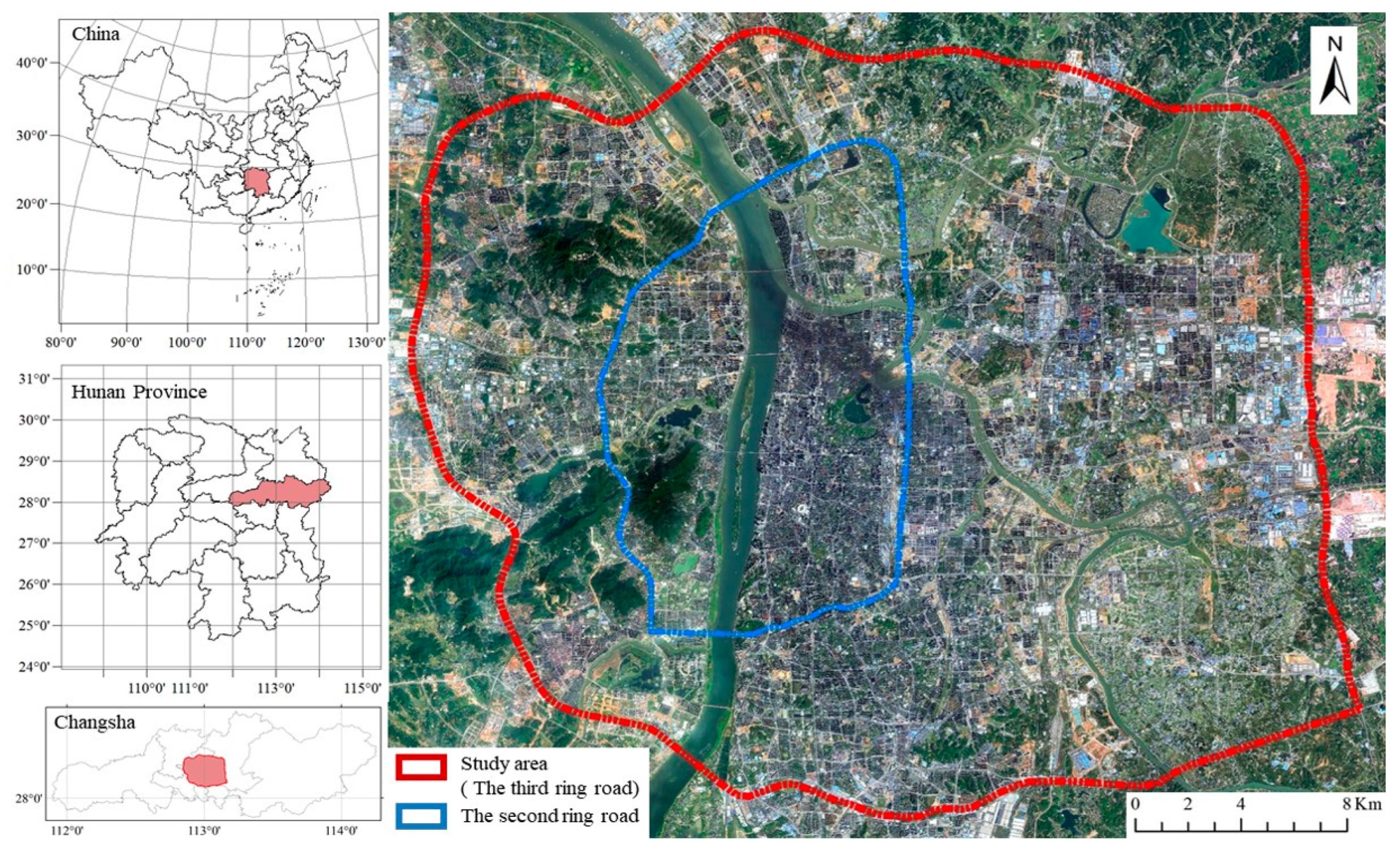
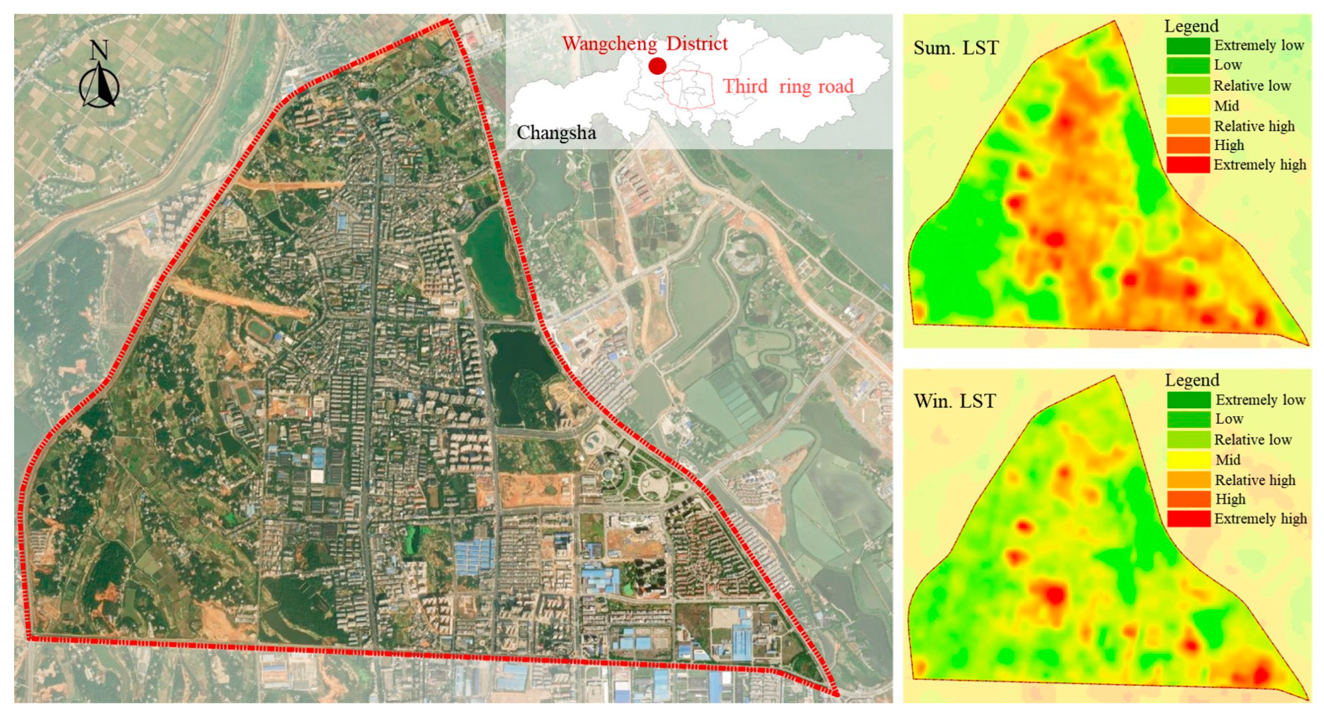
2.1. Study Area
2.2. Data
2.3. Methods
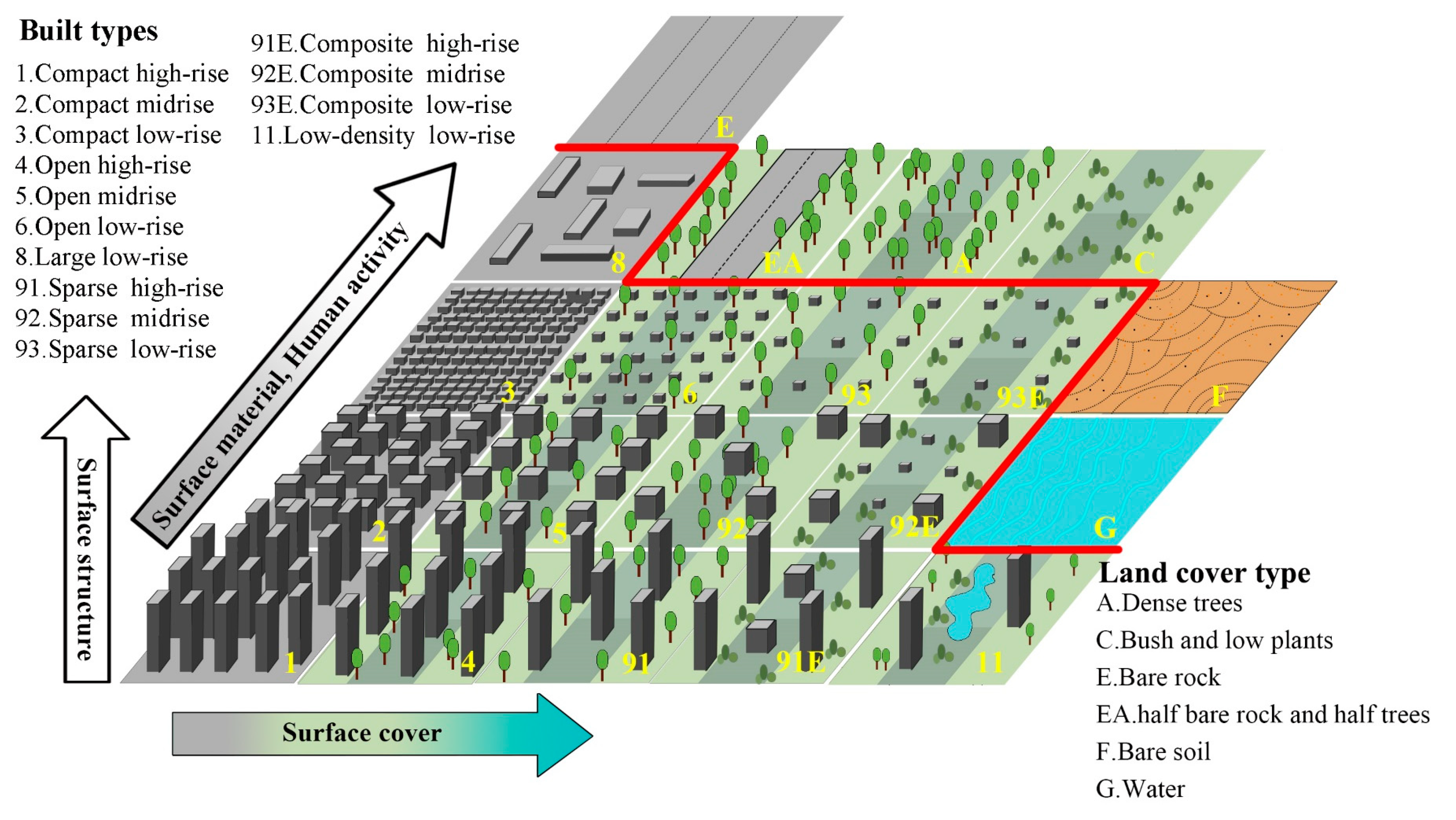
2.3.1. LCZ Mapping
LCZ Parameters
Classification Procedure
LCZ Raster
2.3.2. LCZ Types Transition
2.3.3. LST Inversion
2.3.4. Surface Urban Heat Island Intensity Calculation
2.3.5. Relevant Models
2.3.6. Estimation Indicators
3. Results
3.1. Construction of the LCZ Classification System for Changsha
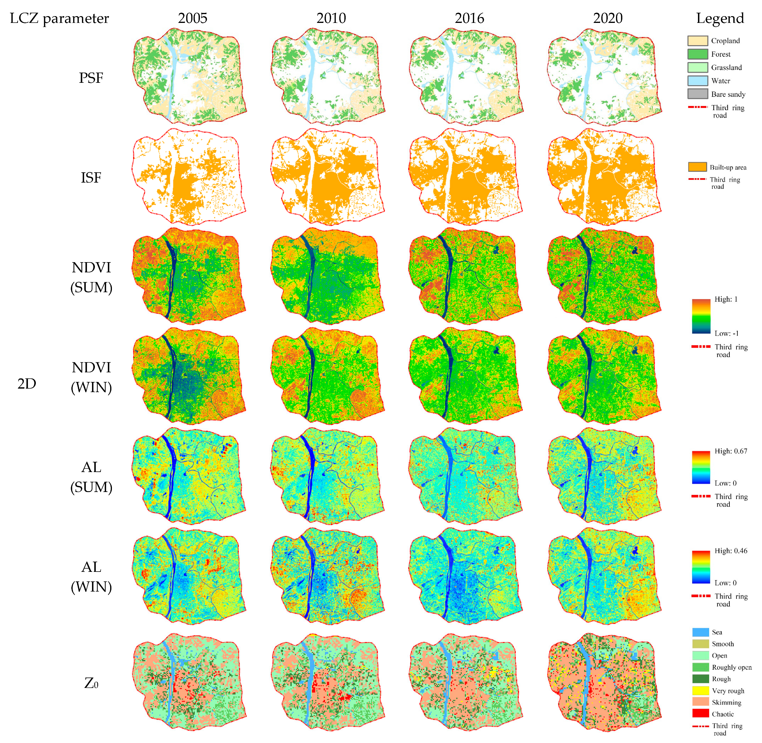
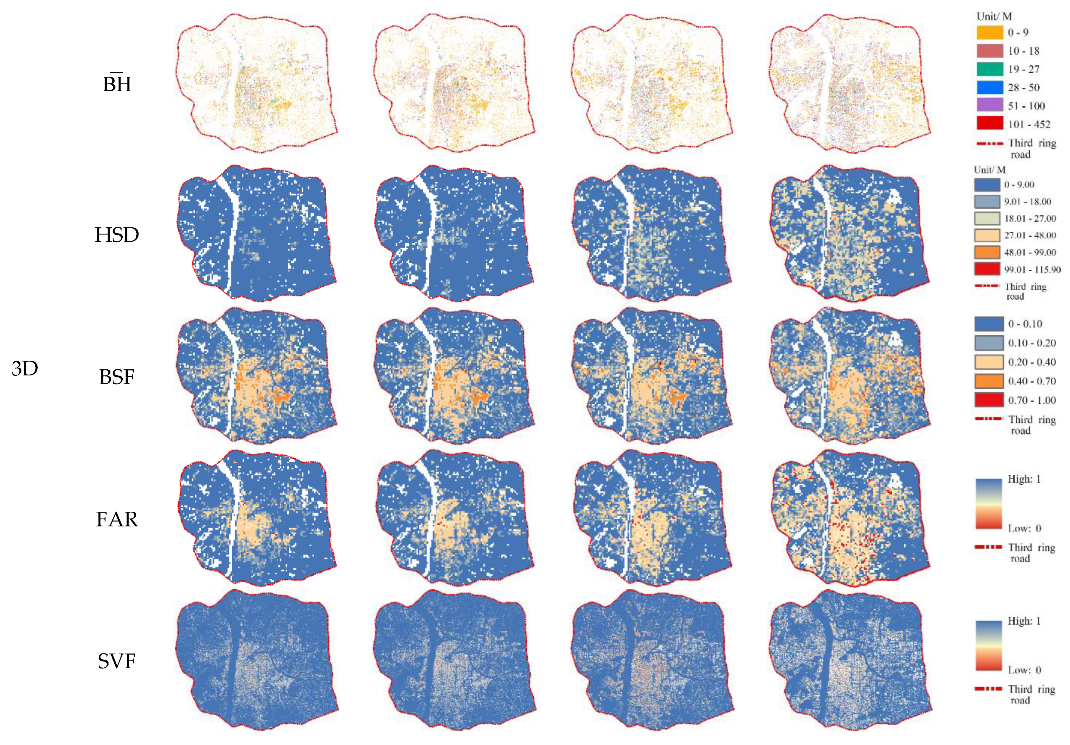
3.1.1. Spatial-Temporal Distribution of the LCZ Parameters
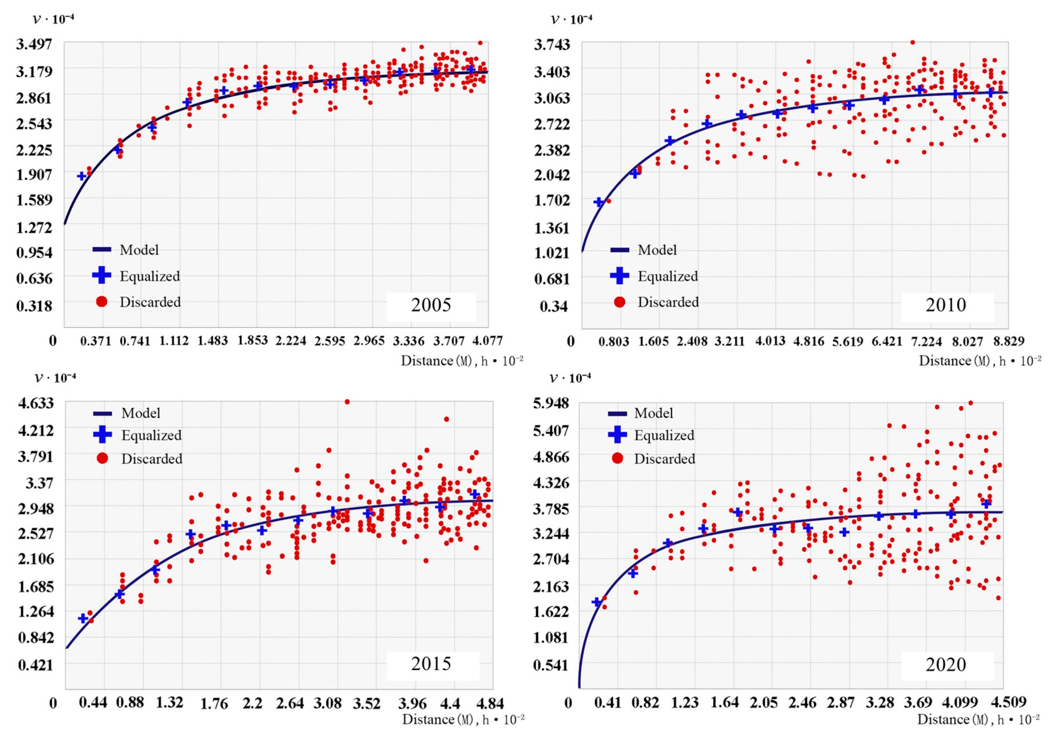
3.1.2. Determining the LCZ Grid Size
3.1.3. Classification System
3.2. General Changes in LCZ
3.2.1. Quantitative Changes
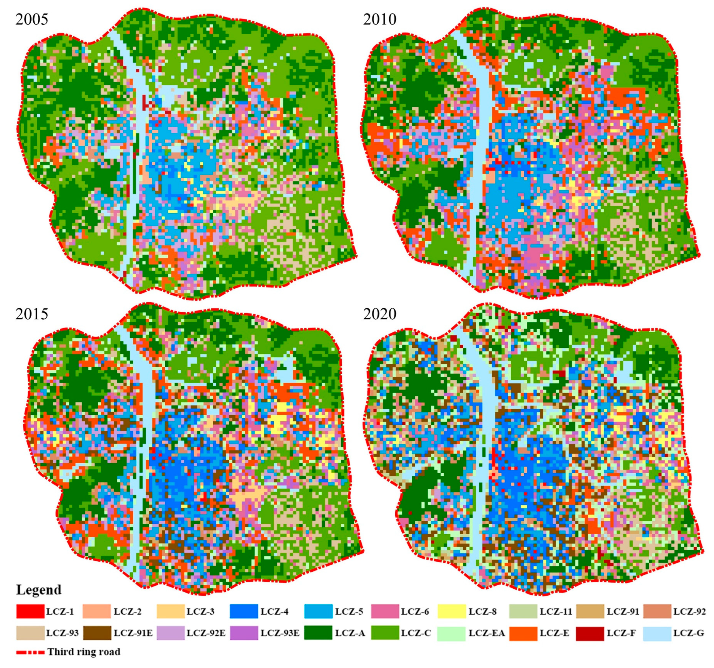
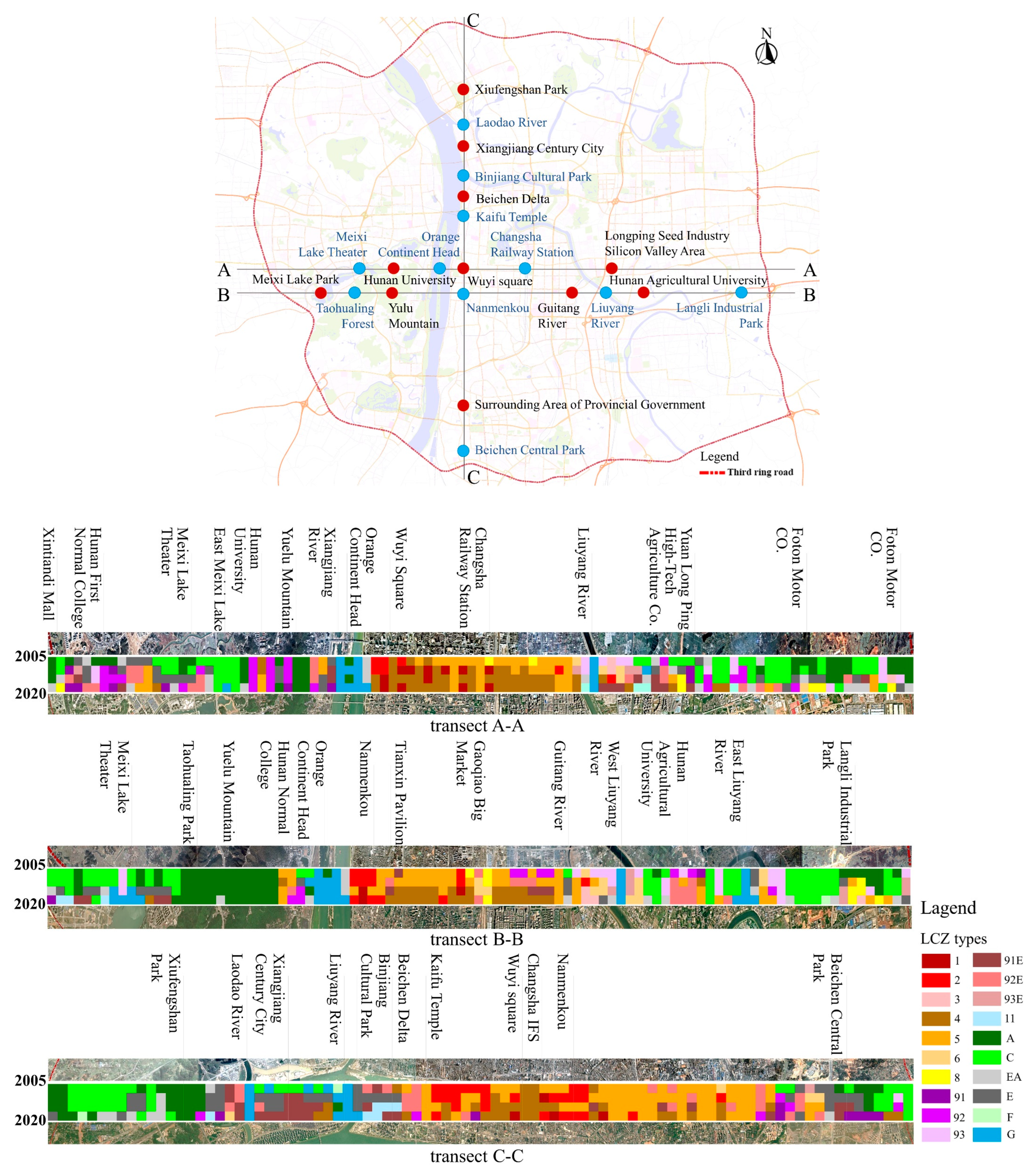
3.2.2. Spatial Layout Changes
3.3. Land Surface Temperature Analysis
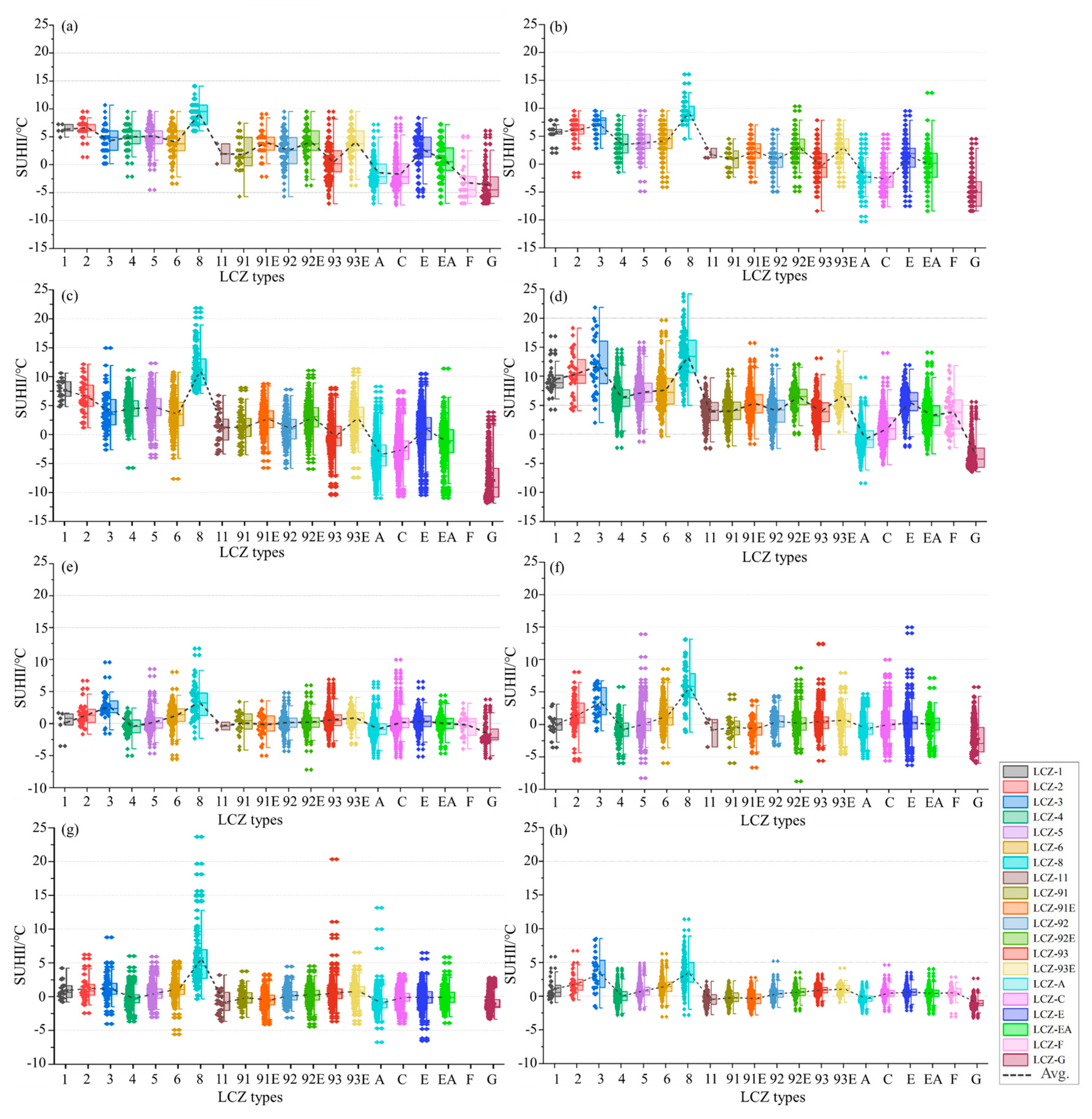
3.4. Relationship between LCZ and SUHII
3.5. The Relative Importance of LCZ Parameters on Seasonal SUHI
3.6. Constructing SUHI Prediction Models
3.6.1. Model Comparison and Analysis
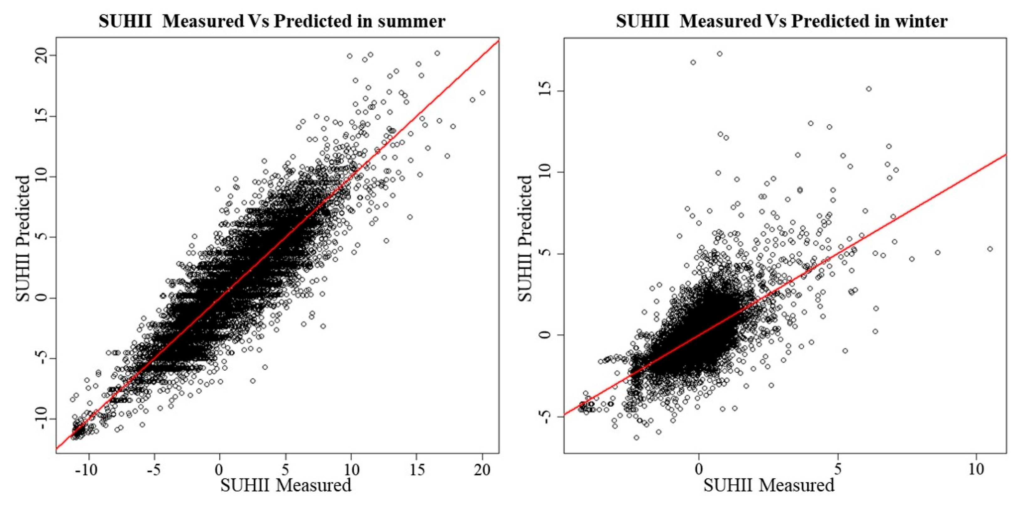
3.6.2. Case Study Validation
4. Discussion
4.1. Spatial-Temporal Evolution Characteristics of the LCZ
4.2. Impact of LCZ Parameter on SUHI
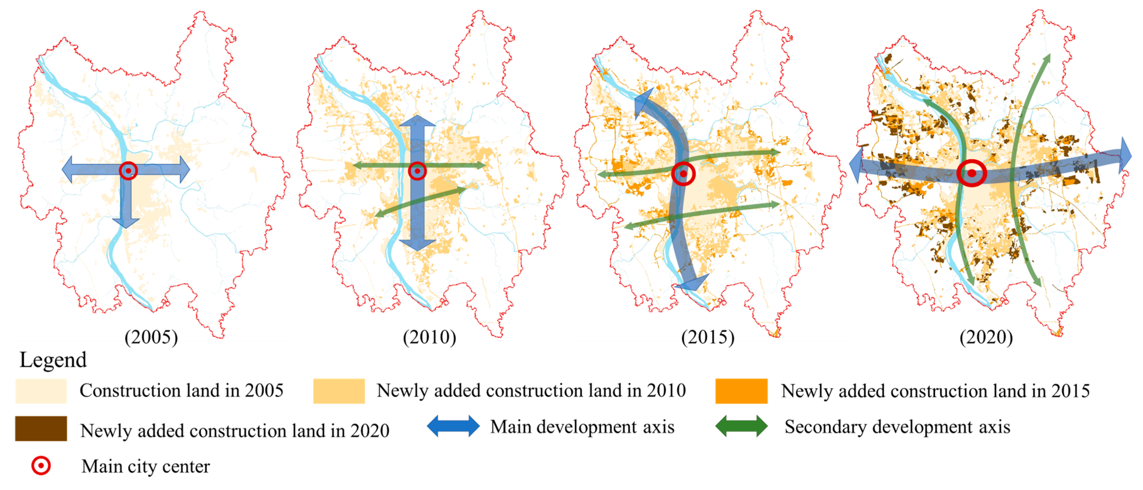
4.3. Impact of Urban Planning
4.4. Limitations
5. Conclusions
Author Contributions
Funding
Data Availability Statement
Conflicts of Interest
Appendix A

| LCZ Class | 2010 | |||||||||||||||||||||
|---|---|---|---|---|---|---|---|---|---|---|---|---|---|---|---|---|---|---|---|---|---|---|
| 1 | 2 | 3 | 4 | 5 | 6 | 8 | 11 | 91 | 92 | 93 | 91E | 92E | 93E | A | C | E | EA | F | G | OA (2005) | ||
| 2005 | 1 | 1 | 2 | 1 | 1 | 5 | ||||||||||||||||
| 2 | 4 | 36 | 1 | 5 | 1 | 4 | 51 | |||||||||||||||
| 3 | 20 | 14 | 13 | 47 | ||||||||||||||||||
| 4 | 2 | 2 | 47 | 26 | 2 | 2 | 2 | 83 | ||||||||||||||
| 5 | 8 | 23 | 2 | 49 | 464 | 20 | 10 | 2 | 4 | 16 | 4 | 1 | 1 | 604 | ||||||||
| 6 | 3 | 8 | 1 | 41 | 183 | 7 | 3 | 6 | 1 | 253 | ||||||||||||
| 8 | 1 | 7 | 8 | 2 | 15 | 10 | 16 | 1 | 3 | 2 | 1 | 66 | ||||||||||
| 11 | 1 | 1 | 2 | |||||||||||||||||||
| 91 | 3 | 3 | 5 | 9 | 2 | 1 | 23 | |||||||||||||||
| 92 | 1 | 3 | 32 | 7 | 2 | 2 | 78 | 3 | 5 | 109 | 2 | 3 | 1 | 9 | 2 | 259 | ||||||
| 93 | 14 | 30 | 1 | 12 | 425 | 26 | 112 | 1 | 5 | 626 | ||||||||||||
| 91E | 7 | 5 | 1 | 27 | 5 | 1 | 46 | |||||||||||||||
| 92E | 1 | 1 | 10 | 63 | 18 | 1 | 11 | 3 | 6 | 165 | 9 | 7 | 1 | 296 | ||||||||
| 93E | 1 | 2 | 9 | 21 | 2 | 10 | 1 | 11 | 83 | 8 | 148 | |||||||||||
| A | 3 | 1 | 11 | 7 | 2 | 5 | 19 | 28 | 10 | 27 | 23 | 1231 | 34 | 239 | 39 | 21 | 1700 | |||||
| C | 6 | 18 | 18 | 2 | 3 | 25 | 43 | 7 | 42 | 30 | 42 | 1740 | 322 | 62 | 42 | 2402 | ||||||
| E | 6 | 20 | 9 | 3 | 1 | 1 | 2 | 11 | 15 | 37 | 24 | 7 | 8 | 190 | 2 | 1 | 337 | |||||
| EA | 2 | 5 | 5 | 4 | 7 | 7 | 2 | 7 | 7 | 9 | 10 | 103 | 23 | 2 | 193 | |||||||
| F | 2 | 28 | 30 | |||||||||||||||||||
| G | 1 | 1 | 3 | 3 | 3 | 1 | 2 | 7 | 10 | 39 | 14 | 321 | 405 | |||||||||
| OA (2010) | 16 | 97 | 36 | 140 | 733 | 332 | 60 | 3 | 24 | 161 | 534 | 89 | 454 | 304 | 1299 | 1804 | 930 | 144 | 0 | 416 | 7576 | |
| LCZ Class | 2015 | ||||||||||||||||||||
|---|---|---|---|---|---|---|---|---|---|---|---|---|---|---|---|---|---|---|---|---|---|
| 1 | 2 | 3 | 4 | 5 | 6 | 8 | 11 | 91 | 92 | 93 | 91E | 92E | 93E | A | C | E | EA | G | OA (2010) | ||
| 2010 | 1 | 5 | 1 | 10 | 16 | ||||||||||||||||
| 2 | 6 | 19 | 25 | 16 | 23 | 3 | 3 | 2 | 97 | ||||||||||||
| 3 | 3 | 6 | 16 | 4 | 1 | 3 | 1 | 2 | 36 | ||||||||||||
| 4 | 2 | 92 | 22 | 2 | 21 | 1 | 140 | ||||||||||||||
| 5 | 2 | 2 | 205 | 360 | 48 | 21 | 1 | 1 | 2 | 41 | 41 | 2 | 7 | 733 | |||||||
| 6 | 1 | 2 | 8 | 38 | 79 | 134 | 19 | 2 | 5 | 14 | 14 | 7 | 9 | 332 | |||||||
| 8 | 2 | 5 | 19 | 3 | 2 | 4 | 21 | 2 | 1 | 1 | 60 | ||||||||||
| 11 | 1 | 1 | 1 | 3 | |||||||||||||||||
| 91 | 3 | 5 | 9 | 1 | 3 | 2 | 1 | 24 | |||||||||||||
| 92 | 1 | 1 | 2 | 6 | 3 | 1 | 16 | 84 | 17 | 3 | 12 | 3 | 5 | 3 | 1 | 2 | 1 | 161 | |||
| 93 | 1 | 3 | 1 | 2 | 18 | 1 | 26 | 75 | 336 | 7 | 6 | 24 | 5 | 19 | 1 | 6 | 3 | 534 | |||
| 91E | 3 | 4 | 2 | 51 | 22 | 1 | 6 | 89 | |||||||||||||
| 92E | 20 | 34 | 7 | 7 | 1 | 1 | 115 | 226 | 29 | 14 | 454 | ||||||||||
| 93E | 2 | 6 | 16 | 9 | 12 | 1 | 1 | 1 | 56 | 79 | 100 | 21 | 304 | ||||||||
| A | 3 | 2 | 3 | 13 | 1 | 5 | 8 | 13 | 16 | 5 | 1 | 3 | 1118 | 7 | 63 | 37 | 1 | 1299 | |||
| C | 11 | 1 | 10 | 26 | 5 | 3 | 3 | 8 | 34 | 8 | 5 | 8 | 18 | 1416 | 133 | 63 | 52 | 1804 | |||
| E | 3 | 11 | 15 | 20 | 33 | 13 | 4 | 8 | 4 | 62 | 39 | 50 | 561 | 107 | 930 | ||||||
| EA | 1 | 2 | 3 | 2 | 1 | 2 | 4 | 4 | 3 | 1 | 2 | 4 | 22 | 93 | 144 | ||||||
| G | 1 | 1 | 1 | 1 | 33 | 2 | 4 | 2 | 371 | 416 | |||||||||||
| OA (2015) | 17 | 39 | 94 | 412 | 583 | 288 | 127 | 34 | 70 | 208 | 417 | 387 | 452 | 228 | 1183 | 1452 | 845 | 312 | 428 | 7576 | |
| LCZ Class | 2020 | |||||||||||||||||||||
|---|---|---|---|---|---|---|---|---|---|---|---|---|---|---|---|---|---|---|---|---|---|---|
| 1 | 2 | 3 | 4 | 5 | 6 | 8 | 11 | 91 | 92 | 93 | 91E | 92E | 93E | A | C | E | EA | F | G | OA (2015) | ||
| 2015 | 1 | 7 | 7 | 3 | 17 | |||||||||||||||||
| 2 | 1 | 12 | 3 | 12 | 2 | 2 | 4 | 1 | 2 | 39 | ||||||||||||
| 3 | 1 | 2 | 9 | 5 | 1 | 4 | 14 | 12 | 2 | 1 | 2 | 14 | 3 | 2 | 7 | 10 | 5 | 94 | ||||
| 4 | 20 | 4 | 341 | 8 | 4 | 5 | 28 | 1 | 1 | 412 | ||||||||||||
| 5 | 2 | 20 | 1 | 81 | 406 | 12 | 6 | 4 | 11 | 1 | 8 | 23 | 1 | 3 | 4 | 583 | ||||||
| 6 | 13 | 13 | 26 | 121 | 16 | 7 | 3 | 2 | 6 | 13 | 4 | 7 | 7 | 25 | 25 | 288 | ||||||
| 8 | 2 | 1 | 12 | 4 | 10 | 24 | 71 | 1 | 2 | 127 | ||||||||||||
| 11 | 5 | 13 | 2 | 13 | 1 | 34 | ||||||||||||||||
| 91 | 10 | 2 | 6 | 20 | 2 | 21 | 1 | 2 | 6 | 70 | ||||||||||||
| 92 | 9 | 13 | 3 | 4 | 18 | 80 | 4 | 11 | 29 | 3 | 12 | 1 | 2 | 18 | 1 | 208 | ||||||
| 93 | 5 | 7 | 63 | 4 | 12 | 14 | 191 | 7 | 4 | 26 | 8 | 21 | 9 | 38 | 3 | 5 | 417 | |||||
| 91E | 110 | 3 | 17 | 50 | 2 | 193 | 2 | 6 | 4 | 387 | ||||||||||||
| 92E | 60 | 80 | 6 | 6 | 5 | 25 | 69 | 2 | 60 | 98 | 4 | 2 | 1 | 17 | 17 | 452 | ||||||
| 93E | 1 | 1 | 18 | 11 | 28 | 9 | 3 | 5 | 11 | 24 | 17 | 7 | 34 | 7 | 25 | 27 | 228 | |||||
| A | 3 | 7 | 9 | 15 | 5 | 19 | 34 | 32 | 38 | 21 | 1 | 1 | 700 | 77 | 10 | 148 | 24 | 39 | 1183 | |||
| C | 2 | 13 | 12 | 17 | 4 | 35 | 51 | 39 | 92 | 34 | 6 | 10 | 188 | 586 | 29 | 272 | 20 | 42 | 1452 | |||
| E | 2 | 68 | 34 | 12 | 8 | 68 | 53 | 25 | 20 | 181 | 23 | 5 | 25 | 25 | 85 | 180 | 7 | 24 | 845 | |||
| EA | 9 | 9 | 5 | 2 | 18 | 17 | 17 | 7 | 23 | 3 | 1 | 30 | 33 | 16 | 72 | 4 | 46 | 312 | ||||
| F | 0 | |||||||||||||||||||||
| G | 8 | 1 | 3 | 4 | 2 | 1 | 1 | 7 | 23 | 2 | 28 | 348 | 428 | |||||||||
| OA (2020) | 33 | 43 | 40 | 768 | 643 | 310 | 143 | 223 | 304 | 308 | 392 | 653 | 205 | 97 | 972 | 790 | 241 | 848 | 59 | 504 | 7576 | |
| LCZ Class | 2020 | |||||||||||||||||||||
|---|---|---|---|---|---|---|---|---|---|---|---|---|---|---|---|---|---|---|---|---|---|---|
| 1 | 2 | 3 | 4 | 5 | 6 | 8 | 11 | 91 | 92 | 93 | 91E | 92E | 93E | A | C | E | EA | F | G | OA (2005) | ||
| 2005 | 1 | 2 | 2 | 1 | 5 | |||||||||||||||||
| 2 | 8 | 12 | 2 | 10 | 10 | 1 | 3 | 3 | 1 | 1 | 51 | |||||||||||
| 3 | 1 | 2 | 4 | 1 | 1 | 5 | 7 | 1 | 13 | 1 | 1 | 7 | 3 | 47 | ||||||||
| 4 | 2 | 2 | 66 | 6 | 2 | 5 | 83 | |||||||||||||||
| 5 | 15 | 12 | 238 | 245 | 18 | 7 | 4 | 4 | 10 | 2 | 31 | 9 | 1 | 1 | 5 | 2 | 604 | |||||
| 6 | 3 | 1 | 5 | 42 | 42 | 43 | 15 | 10 | 5 | 1 | 30 | 6 | 5 | 4 | 24 | 17 | 253 | |||||
| 8 | 1 | 4 | 3 | 19 | 9 | 1 | 11 | 1 | 4 | 2 | 1 | 7 | 1 | 1 | 1 | 66 | ||||||
| 11 | 1 | 1 | 2 | |||||||||||||||||||
| 91 | 3 | 3 | 1 | 4 | 5 | 1 | 4 | 1 | 1 | 23 | ||||||||||||
| 92 | 2 | 41 | 34 | 11 | 1 | 2 | 26 | 43 | 5 | 46 | 18 | 5 | 7 | 1 | 6 | 11 | 259 | |||||
| 93 | 2 | 4 | 29 | 33 | 66 | 2 | 24 | 28 | 36 | 174 | 39 | 20 | 27 | 7 | 29 | 30 | 67 | 3 | 6 | 626 | ||
| 91E | 15 | 5 | 2 | 2 | 5 | 2 | 9 | 5 | 1 | 46 | ||||||||||||
| 92E | 1 | 58 | 75 | 3 | 4 | 3 | 17 | 31 | 3 | 56 | 34 | 3 | 2 | 3 | 3 | 296 | ||||||
| 93E | 1 | 23 | 16 | 17 | 8 | 2 | 8 | 8 | 3 | 27 | 13 | 4 | 1 | 1 | 6 | 9 | 1 | 148 | ||||
| A | 5 | 5 | 67 | 48 | 46 | 32 | 38 | 68 | 69 | 60 | 121 | 20 | 7 | 729 | 90 | 34 | 211 | 25 | 25 | 1700 | ||
| C | 2 | 3 | 11 | 100 | 71 | 80 | 48 | 84 | 100 | 72 | 119 | 161 | 48 | 35 | 200 | 635 | 75 | 399 | 27 | 132 | 2402 | |
| E | 3 | 31 | 33 | 16 | 7 | 16 | 18 | 17 | 10 | 61 | 13 | 8 | 12 | 3 | 21 | 49 | 3 | 16 | 337 | |||
| EA | 2 | 14 | 10 | 4 | 2 | 13 | 8 | 9 | 8 | 23 | 12 | 9 | 12 | 11 | 39 | 17 | 193 | |||||
| F | 1 | 2 | 2 | 25 | 30 | |||||||||||||||||
| G | 5 | 1 | 1 | 1 | 12 | 3 | 4 | 4 | 19 | 4 | 5 | 12 | 16 | 35 | 1 | 282 | 405 | |||||
| OA (2020) | 33 | 43 | 40 | 768 | 643 | 310 | 143 | 223 | 304 | 308 | 392 | 653 | 205 | 97 | 972 | 790 | 241 | 848 | 59 | 504 | 7576 | |
Appendix B
| Land Cover | 2005 | 2010 | 2015 | 2020 | |||||
|---|---|---|---|---|---|---|---|---|---|
| PSF | Cropland | 268.15 | 39.43% | 185.18 | 27.23% | 156.55 | 23.02% | 93.37 | 13.73% |
| Forest | 169.61 | 24.94% | 134.92 | 19.84% | 126.90 | 18.66% | 122.27 | 17.98% | |
| Grassland | 1.97 | 0.29% | 1.70 | 0.25% | 1.43 | 0.21% | 1.16 | 0.17% | |
| Water | 47.54 | 6.99% | 43.73 | 6.43% | 43.25 | 6.36% | 42.23 | 6.21% | |
| Barren | 3.33 | 0.49% | 0 | 0 | 0 | 0 | 32.98 | 4.85% | |
| Overall | 490.60 | 72.14% | 365.53 | 53.75% | 328.13 | 48.25% | 292.02 | 42.94% | |
| ISF | 189.46 | 27.86% | 314.53 | 46.25% | 351.93 | 51.75% | 388.04 | 57.06% | |
References
- Masson-Delmotte, V.; Pörtner, H.O.; Skea, J.; Zhai, P.; Roberts, D. Special Report: Global Warming of 1.5 °C; Intergovernmental Panel on Climate Change (IPCC): New York, NY, USA, 2019. [Google Scholar]
- China Meteorological Administration. Blue Book on Climate Change in China 2023; Science Press: Beijing, China, 2023.
- Aerospace Information Research Institute, Chinese Academy of Sciences. Remote Sensing Monitoring Database for the Expansion of Typical Cities in China in the Past 50 Years. Available online: https://aircas.cas.cn/dtxw/kydt/202103/t20210304_5969166.html (accessed on 8 August 2023).
- He, B.; Wang, J.; Zhu, J.; Qi, J. Beating the urban heat: Situation, background, impacts and the way forward in China. Renew. Sustain. Energy Rev. 2022, 161, 112350. [Google Scholar] [CrossRef]
- Schwarz, N.; Schlink, U.; Franck, U.; Großmann, K. Relationship of land surface and air temperatures and its implications for quantifying urban heat island indicators—An application for the city of Leipzig (Germany). Ecol. Indic. 2012, 18, 693–704. [Google Scholar] [CrossRef]
- Sheng, L.; Tang, X.; You, H.; Gu, Q.; Hu, H. Comparison of the urban heat island intensity quantified by using air temperature and Landsat land surface temperature in Hangzhou, China. Ecol. Indic. 2017, 72, 738–746. [Google Scholar] [CrossRef]
- Kikon, N.; Singh, P.; Singh, S.K.; Vyas, A. Assessment of urban heat islands (UHI) of Noida City, India using multi-temporal satellite data. Sustain. Cities Soc. 2016, 22, 19–28. [Google Scholar] [CrossRef]
- dos Santos, A.R.; de Oliveira, F.S.; da Silva, A.G.; Gleriani, J.M.; Gonçalves, W.; Moreira, G.L.; Silva, F.G.; Branco, E.R.F.; Moura, M.M.; da Silva, R.G.; et al. Spatial and temporal distribution of urban heat islands. Sci. Total Environ. 2017, 605–606, 946–956. [Google Scholar] [CrossRef]
- Tao, S.; Ranhao, S.; Liding, C. The Trend Inconsistency between Land Surface Temperature and Near Surface Air Temperature in Assessing Urban Heat Island Effects. Remote Sens. 2020, 12, 1271. [Google Scholar] [CrossRef]
- Xiang, Y.; Zheng, B.; Bedra, K.B.; Ouyang, Q.; Liu, J.; Zheng, J. Spatial and seasonal differences between near surface air temperature and land surface temperature for Urban Heat Island effect assessment. Urban Clim. 2023, 52, 101745. [Google Scholar] [CrossRef]
- Stewart, I.D.; Oke, T.R. Local Climate Zones for Urban Temperature Studies. Bull. Amer. Meteor. Soc. 2012, 93, 1879–1900. [Google Scholar] [CrossRef]
- Bechtel, B.; Alexander, P.J.; Beck, C.; Böhner, J.; Brousse, O.; Ching, J.; Demuzere, M.; Fonte, C.; Gál, T.; Hidalgo, J.; et al. Generating WUDAPT Level 0 data—Current status of production and evaluation. Urban Clim. 2019, 27, 24–45. [Google Scholar] [CrossRef]
- Yoo, C.; Han, D.; Im, J.; Bechtel, B. Comparison between convolutional neural networks and random forest for local climate zone classification in mega urban areas using Landsat images. ISPRS J. Photogramm. Remote Sens. 2019, 157, 155–170. [Google Scholar] [CrossRef]
- Zheng, Y.; Ren, C.; Xu, Y.; Wang, R.; Ho, J.; Lau, K.; Ng, E. GIS-based mapping of Local Climate Zone in the high-density city of Hong Kong. Urban Clim. 2018, 24, 419–448. [Google Scholar] [CrossRef]
- Gál, T.; Bechtel, B.; Unger, J. Comparison of two different Local Climate Zone mapping methods. In Proceedings of the ICUC9—9th International Conference on Urban Climate Jointly with 12th Symposium on the Urban Environment, Toulouse, France, 20–24 July 2015. [Google Scholar]
- Ren, C.; Wang, R.; Cai, M.; Xu, Y.; Ng, E. The Accuracy of LCZ maps Generated by the World Urban Database and Access Portal Tools (WUDAPT) Method: A Case Study of Hong Kong. In Proceedings of the 4th Countering Urban Heat Island (Uhi) and Climate Change Through Mitigation and Adaptation, Singapore, 30 May–1 June 2016. [Google Scholar]
- Wang, R.; Ren, C.; Xu, Y.; Lau, K.K.; Shi, Y. Mapping the local climate zones of urban areas by GIS-based and WUDAPT methods: A case study of Hong Kong. Urban Clim. 2018, 24, 567–576. [Google Scholar] [CrossRef]
- Han, J.; Liu, J.; Liu, L.; Ye, Y. Spatiotemporal Changes in the Urban Heat Island Intensity of Distinct Local Climate Zones: Case Study of Zhongshan District, Dalian, China. Complexity 2020, 8820338. [Google Scholar] [CrossRef]
- Wang, R.; Voogt, J.; Ren, C.; Ng, E. Spatial-temporal variations of surface urban heat island: An application of local climate zone into large Chinese cities. Build. Environ. 2022, 222, 109378. [Google Scholar] [CrossRef]
- Chen, Y.; Hu, Y. The urban morphology classification under local climate zone scheme based on the improved method—A case study of Changsha, China. Urban Clim. 2022, 45, 101271. [Google Scholar] [CrossRef]
- Ren, C.; Cai, M.; Li, X.; Zhang, L.; Wang, R.; Xu, Y.; Ng, E. Assessment of Local Climate Zone Classification Maps of Cities in China and Feasible Refinements. Sci. Rep. 2019, 9, 18848. [Google Scholar] [CrossRef]
- Han, B.; Luo, Z.; Liu, Y.; Zhang, T.; Yang, L. Using Local Climate Zones to investigate Spatio-temporal evolution of thermal environment at the urban regional level: A case study in Xi’an, China. Sustain. Cities Soc. 2022, 76, 103495. [Google Scholar] [CrossRef]
- Geletič, J.; Lehnert, M.; Dobrovolný, P. Land Surface Temperature Differences within Local Climate Zones, Based on Two Central European Cities. Remote Sens. 2016, 8, 788. [Google Scholar] [CrossRef]
- Das, M.; Das, A. Assessing the relationship between local climatic zones (LCZs) and land surface temperature (LST)—A case study of Sriniketan-Santiniketan Planning Area (SSPA), West Bengal, India. Urban Clim. 2020, 32, 100591. [Google Scholar] [CrossRef]
- Hu, J.; Yang, Y.; Pan, X.; Zhu, Q.; Zhan, W.; Wang, Y.; Ma, W. Analysis of the Spatial and Temporal Variations of Land Surface Temperature Based on Local Climate Zones: A Case Study in Nanjing, China. IEEE J. Sel. Top. Appl. Earth Obs. Remote Sens. 2019, 12, 4213–4223. [Google Scholar] [CrossRef]
- Lin, Z.; Xu, H.; Yao, X.; Yang, C.; Yang, L. Exploring the relationship between thermal environmental factors and land surface temperature of a “furnace city” based on local climate zones. Build. Environ. 2023, 243, 110732. [Google Scholar] [CrossRef]
- Yu, Z.; Jing, Y.; Yang, G.; Sun, R. A New Urban Functional Zone-Based Climate Zoning System for Urban Temperature Study. Remote Sens. 2021, 13, 251. [Google Scholar] [CrossRef]
- Middel, A.; Häb, K.; Brazel, A.J.; Martin, C.A.; Guhathakurta, S. Impact of urban form and design on mid-afternoon microclimate in Phoenix Local Climate Zones. Landsc. Urban Plan. 2014, 122, 16–28. [Google Scholar] [CrossRef]
- Chen, W.; Zhang, J.; Shi, X.; Liu, S. Impacts of Building Features on the Cooling Effect of Vegetation in Community-Based MicroClimate: Recognition, Measurement and Simulation from a Case Study of Beijing. IJERPH 2020, 17, 8915. [Google Scholar] [CrossRef] [PubMed]
- Qiao, Z.; Xu, X.; Wu, F.; Luo, W.; Wang, F.; Liu, L.; Sun, Z. Urban ventilation network model: A case study of the core zone of capital function in Beijing metropolitan area. J. Clean. Prod. 2017, 168, 526–535. [Google Scholar] [CrossRef]
- Han, D.; An, H.; Wang, F.; Xu, X.; Qiao, Z.; Wang, M.; Sui, X.; Liang, S.; Hou, X.; Cai, H.; et al. Understanding seasonal contributions of urban morphology to thermal environment based on boosted regression tree approach. Build. Environ. 2022, 226, 109770. [Google Scholar] [CrossRef]
- Li, H.; Li, Y.; Wang, T.; Wang, Z.; Gao, M.; Shen, H. Quantifying 3D building form effects on urban land surface temperature and modeling seasonal correlation patterns. Build. Environ. 2021, 204, 108132. [Google Scholar] [CrossRef]
- Hu, Y.; Dai, Z.; Guldmann, J. Modeling the impact of 2D/3D urban indicators on the urban heat island over different seasons: A boosted regression tree approach. J. Environ. Manag. 2020, 266, 110424. [Google Scholar] [CrossRef]
- Chen, J.; Zhan, W.; Du, P.; Li, L.; Li, J.; Liu, Z.; Huang, F.; Lai, J.; Xia, J. Seasonally disparate responses of surface thermal environment to 2D/3D urban morphology. Build. Environ. 2022, 214, 108928. [Google Scholar] [CrossRef]
- Wang, Q.; Wang, X.; Meng, Y.; Zhou, Y.; Wang, H. Exploring the impact of urban features on the spatial variation of land surface temperature within the diurnal cycle. Sustain. Cities Soc. 2023, 91, 104432. [Google Scholar] [CrossRef]
- Li, Z.; Hu, D. Exploring the relationship between the 2D/3D architectural morphology and urban land surface temperature based on a boosted regression tree: A case study of Beijing, China. Sustain. Cities Soc. 2022, 78, 103392. [Google Scholar] [CrossRef]
- Xu, H.; Li, C.; Hu, Y.; Li, S.; Kong, R.; Zhang, Z. Quantifying the effects of 2D/3D urban landscape patterns on land surface temperature: A perspective from cities of different sizes. Build. Environ. 2023, 233, 110085. [Google Scholar] [CrossRef]
- Xu, Y.; Zhang, C.; Hou, W. Modeling of Daytime and Nighttime Surface Urban Heat Island Distribution Combined with LCZ in Beijing, China. Land 2022, 11, 2050. [Google Scholar] [CrossRef]
- Yu, S.; Chen, Z.; Yu, B.; Wang, L.; Wu, B.; Wu, J.; Zhao, F. Exploring the relationship between 2D/3D landscape pattern and land surface temperature based on explainable eXtreme Gradient Boosting tree: A case study of Shanghai, China. Sci. Total Environ. 2020, 725, 138229. [Google Scholar] [CrossRef] [PubMed]
- Alahuhta, J.; Antikainen, H.; Hjort, J.; Helm, A.; Heino, J. Current climate overrides historical effects on species richness and range size of freshwater plants in Europe and North America. J. Ecol. 2020, 108, 1262–1275. [Google Scholar] [CrossRef]
- Han, D.; An, H.; Cai, H.; Wang, F.; Xu, X.; Qiao, Z.; Jia, K.; Sun, Z.; An, Y. How do 2D/3D urban landscapes impact diurnal land surface temperature: Insights from block scale and machine learning algorithms. Sustain. Cities Soc. 2023, 99, 104933. [Google Scholar] [CrossRef]
- Changsha Municipal, Gov. Overview of Changsha. Available online: http://www.changsha.gov.cn/xfzs/zjmlzs/zsgl/200907/t20090727_5686409.html?eqid=dab79ba600213c5a0000000664552691 (accessed on 24 May 2024).
- Beck, H.E.; McVicar, T.R.; Vergopolan, N.; Berg, A.; Lutsko, N.J.; Dufour, A.; Zeng, Z. High-resolution (1 km) Köppen-Geiger maps for 1901–2099 based on constrained CMIP6 projections. Sci. Data 2023, 10, 724. [Google Scholar] [CrossRef]
- Hunan Meteorological Bureau. The Hot and Humid Competition in North China, Northeast China, and Many Places in Jiangnan May Break Records again due to High Temperatures. Available online: http://hn.cma.gov.cn/xwzx/tqzx/201808/t20180801_841310.html (accessed on 8 August 2023).
- Colaninno, N.; Morello, E. Towards an operational model for estimating day and night instantaneous near-surface air temperature for urban heat island studies: Outline and assessment. Urban Clim. 2022, 46, 101320. [Google Scholar] [CrossRef]
- Qin, J.; He, M.; Jiang, H.; Lu, N. Reconstruction of 60-year (1961–2020) surface air temperature on the Tibetan Plateau by fusing MODIS and ERA5 temperatures. Sci. Total Environ. 2022, 853, 158406. [Google Scholar] [CrossRef]
- Li, Z.H.; He, W.; Cheng, M.; Hu, J.X.; Yang, G.Y.; Zhang, H.Y. SinoLC-1: The first 1 m resolution national-scale land-cover map of China created with a deep learning framework and open-access data. Earth Syst. Sci. Data 2023, 15, 4749–4780. Available online: https://zenodo.org/records/8214871 (accessed on 8 August 2023). [CrossRef]
- Shi, Q.; Liu, M.X.; Marinoni, A.; Liu, X. UGS-1m: Fine-grained urban green space mapping of 31 major cities in China based on the deep learning framework. Sci. Data Bank 2023. [Google Scholar] [CrossRef]
- Liang, S. Narrowband to broadband conversions of land surface albedo I: Algorithms. Remote Sens. Environ. 2001, 76, 213–238. [Google Scholar] [CrossRef]
- Davenport, A.G.; Grimmond, C.; Oke, T.R.; Wiering, J. Estimating the roughness of cities and sheltered country. In Proceedings of the 12th Conference on Applied Climatology, Asheville, NC, USA, 8–12 May 2000; pp. 96–99. [Google Scholar]
- Huang, S.; Tang, L.; Hupy, J.P.; Wang, Y.; Shao, G. A commentary review on the use of normalized difference vegetation index (NDVI) in the era of popular remote sensing. J. For. Res. 2021, 32, 1–6. [Google Scholar] [CrossRef]
- Miao, C.; Yu, S.; Hu, Y.; Zhang, H.; He, X.; Chen, W. Review of methods used to estimate the sky view factor in urban street canyons. Build. Environ. 2020, 168, 106497. [Google Scholar] [CrossRef]
- Yang, J.; Yang, Y.; Sun, D.; Jin, C.; Xiao, X. Influence of urban morphological characteristics on thermal environment. Sustain. Cities Soc. 2021, 72, 103045. [Google Scholar] [CrossRef]
- Lan, Y.; Zhan, Q. How do urban buildings impact summer air temperature? The effects of building configurations in space and time. Build. Environ. 2017, 125, 88–98. [Google Scholar] [CrossRef]
- Huang, F.; Jiang, S.; Zhan, W.; Bechtel, B.; Liu, Z.; Demuzere, M.; Huang, Y.; Xu, Y.; Ma, L.; Xia, W.; et al. Mapping local climate zones for cities: A large review. Remote Sens. Environ. 2023, 292, 113573. [Google Scholar] [CrossRef]
- Houet, T.; Pigeon, G. Mapping urban climate zones and quantifying climate behaviors—An application on Toulouse urban area (France). Environ. Pollut. 2011, 159, 2180–2192. [Google Scholar] [CrossRef]
- Thomas, L.; Grimmond, C.S.B. Characterization of Energy Flux Partitioning in Urban Environments: Links with Surface Seasonal Properties. J. Appl. Meteorol. Clim. 2012, 51, 219–241. [Google Scholar]
- Rodler, A.; Leduc, T. Local climate zone approach on local and micro scales: Dividing the urban open space. Urban Clim. 2019, 28, 100457. [Google Scholar] [CrossRef]
- Zheng, Z.; Luo, F.; Li, N.; Gao, H.; Yang, Y. Impact of Local Climate Zones on the Urban Heat and Dry Islands in Beijing: Spatial Heterogeneity and Relative Contributions. J. Meteorol. Res. 2024, 38, 126–137. [Google Scholar] [CrossRef]
- Li, X.; Yeh, A.G. Neural-network-based cellular automata for simulating multiple land use changes using GIS. Int. J. Geogr. Inf. Sci. 2002, 16, 323–343. [Google Scholar] [CrossRef]
- Tang, B.H.; Zhan, C.; Li, Z.L.; Wu, H.; Tang, R. Estimation of Land Surface Temperature from MODIS Data for the Atmosphere with Air Temperature Inversion Profile. IEEE J. Sel. Top. Appl. Earth Obs. Remote Sens. 2017, 10, 2976–2983. [Google Scholar] [CrossRef]
- Rongali, G.; Keshari, A.K.; Gosain, A.K.; Khosa, R. A Mono-Window Algorithm for Land Surface Temperature Estimation from Landsat 8 Thermal Infrared Sensor Data: A Case Study of the Beas River Basin, India. Pertanika J. Sci. Technol. 2018, 26, 829–840. [Google Scholar]
- Song, T.; Duan, Z.; Liu, J.; Shi, J.; Yan, F.; Sheng, S. Comparison of four algorithms to retrieve land surface temperature using Landsat 8 satellite. Natl. Remote Sens. Bull. 2015, 19, 451–464. [Google Scholar]
- Elith, J.; Leathwick, J.R.; Hastie, T. A working guide to boosted regression trees. J. Anim. Ecol. 2008, 77, 802–813. [Google Scholar] [CrossRef]
- Hair, J.F.; Black, W.C.; Babin, B.J.; Anderdon, R.E. Multivariate Data Analysis, 7th ed.; Prentice Hall: Upper Saddle River, NJ, USA, 2009. [Google Scholar]
- Wang, R.; Cai, M.; Ren, C.; Bechtel, B.; Xu, Y.; Ng, E. Detecting multi-temporal land cover change and land surface temperature in Pearl River Delta by adopting local climate zone. Urban Clim. 2019, 28, 100455. [Google Scholar] [CrossRef]
- Guo, G.; Zhou, X.; Wu, Z.; Xiao, R.; Chen, Y. Characterizing the impact of urban morphology heterogeneity on land surface temperature in Guangzhou, China. Environ. Model. Softw. 2016, 84, 427–439. [Google Scholar] [CrossRef]
- United Nations Department of Economic and Social Affairs. 68% of the World Population Projected to Live in Urban Areas by 2050, Says UN.; Revision of World Urbanization Prospects; United Nations: New York, NY, USA, 2018. [Google Scholar]
- Gong, Y.; Li, X.; Liu, H.; Li, Y. The Spatial Pattern and Mechanism of Thermal Environment in Urban Blocks from the Perspective of Green Space Fractal. Buildings 2023, 13, 574. [Google Scholar] [CrossRef]
- Naeem, S.; Naeem, S.; Naeem, S.; Cao, C.; Qazi, W.A.; Zamani, M.; Wei, C.; Acharya, B.K.; Rehman, A.U. Studying the Association between Green Space Characteristics and Land Surface Temperature for Sustainable Urban Environments: An Analysis of Beijing and Islamabad. ISPRS Int. J. Geo-Inf. 2018, 7, 38. [Google Scholar] [CrossRef]
- Turhan, C.; Özbey, M.F.; Lotfi, B.; Gökçen Akkurt, G. Integration of psychological parameters into a thermal sensation prediction model for intelligent control of the HVAC systems. Energy Build. 2023, 296, 113404. [Google Scholar] [CrossRef]


| Year | Satellite Model | Season | Data (m/d) | WRS Path/Row | Sun-Elevation | Sun-Azimuth | Land Cloud Cover |
|---|---|---|---|---|---|---|---|
| 2005 | Landsat 7 | Summer | 8/2 | 123/40 | 63.15357870 | 108.55007428 | 4.00 |
| 8/2 | 123/41 | 63.35264972 | 105.55576563 | 3.00 | |||
| Winter | 12/8 | 123/40 | 33.84027840 | 154.27640755 | 0.00 | ||
| 12/8 | 123/41 | 35.02755534 | 153.57313566 | 0.00 | |||
| 2010 | Landsat 5 | Summer | 8/21 | 123/40 | 60.68345466 | 119.52856771 | 4.00 |
| 8/21 | 123/41 | 61.15568514 | 116.93293115 | 2.00 | |||
| Landsat 7 | Winter | 12/22 | 123/40 | 32.94643872 | 153.95202880 | 0.00 | |
| 12/22 | 123/41 | 34.13052128 | 153.26324036 | 1.00 | |||
| 2016 | Landsat 8–9 | Summer | 7/23 | 123/40 | 66.49031153 | 106.76246786 | 1.63 |
| 7/23 | 123/41 | 66.63615756 | 103.29242434 | 3.11 | |||
| Winter | 12/30 | 123/40 | 33.48688786 | 154.53316225 | 3.94 | ||
| 12/30 | 123/41 | 34.67955246 | 153.84089683 | 0.15 | |||
| 2020 | Landsat 8–9 | Summer | 8/3 | 123/40 | 65.27432146 | 112.38536985 | 5.61 |
| 8/3 | 123/41 | 65.56427737 | 109.13729274 | 8.04 | |||
| Winter | 12/25 | 123/40 | 33.50019512 | 155.29162805 | 0.22 | ||
| 12/25 | 123/41 | 34.70360411 | 154.60980959 | 0.44 |
| Parameter | Description | Formula | |
|---|---|---|---|
| 2D | PSF [26] | Proportional pervious surface area of a grid. | where PSA is the pervious surface area, and Ai is the grid area of grid number i. |
| ISF [26] | Proportional impervious surface area of a grid. | where ISA is impervious surface area, and Ai is the grid area of grid number i. | |
| AL [49] | Represents the heat balance on the Earth’s surface. | where ρ represents Landsat bands 1, 3, 4, 5 and 7. | |
| Z0 [50] | Roughness length describing the terrain surface (building geometry and land cover). | The roughness length is classified according to the classification system proposed by Davenport et al. | |
| NDVI [51] | It is effective for expressing vegetation status and quantified vegetation attributes. | where Red and NIR are spectral radiance (or reflectance) measurements recorded with sensors in red (visible) and NIR regions, respectively. | |
| 3D | SVF [52,53] | The fraction of the overlying hemisphere occupied by the sky. | where αi is the azimuth angle, and βi is the maximum tilt angle along the pixel direction of the obstruction. |
| B͞H | The weighted average height of buildings in the grid. | where i is the building number, n is the total number of buildings in the grid, H is the building height, and Wi is the weight value of the total building area of building number i in the grid area. | |
| HSD [26] | Variation degree of the building height of a grid. | where i is the building number, n is the total number of buildings in the grid, H is the building height and is the average building height. | |
| BSF [32] | The ratio of the footprint area of buildings to the total area of the grid. | where i is the building number, Aarc is the footprint area of the i building, j is the grid number, and Aj is the grid area of grid number j. | |
| FAR [54] | The ratio of the floor area of the buildings to the total area of the grid. | where i is the building number, Aarc is the footprint area of the i building, F is the number of floors of building number i, j is the grid number, and Aj is the grid area of grid number j. | |
| 1 | 2 | 3 | 4 | 5 | 6 | 8 | 11 | 91 | 92 | 93 | 91E | 92E | 93E | A | C | E | EA | F | G | Overall Change | ||
|---|---|---|---|---|---|---|---|---|---|---|---|---|---|---|---|---|---|---|---|---|---|---|
| Built LCZs | Land Cover LCZs | |||||||||||||||||||||
| 2005 | 0.07 | 0.66 | 0.61 | 1.08 | 7.87 | 3.30 | 0.86 | 0.30 | 3.38 | 8.21 | 0.60 | 3.86 | 1.94 | 0.03 | 22.62 | 31.87 | 2.57 | 4.47 | 0.40 | 5.30 | 32.77 | 67.23 |
| 2010 | 0.14 | 0.6 | −0.14 | 0.74 | 1.68 | 1.03 | −0.08 | 0.01 | 0.01 | −1.28 | −1.19 | 0.56 | 2.06 | 2.07 | −5.3 | −7.97 | −0.6 | 7.9 | −0.4 | 0.16 | 38.98 | 61.02 |
| 2015 | 0.15 | −0.15 | 0.61 | 4.29 | −0.27 | 0.58 | 0.66 | 0.41 | 0.61 | −0.66 | −2.72 | 4.44 | 2.03 | 1.11 | −6.89 | −12.61 | 1.63 | 6.85 | −0.4 | 0.16 | 43.86 | 56.14 |
| 2020 | 0.36 | −0.01 | −0.06 | 8.93 | 0.57 | 1.23 | 0.34 | 2.88 | 3.67 | 0.65 | −3.04 | 7.91 | −1.16 | −0.66 | −13.69 | −25.45 | 0.82 | 16.68 | 0.15 | −0.43 | 54.38 | 45.62 |
| LST Class | 2005 | 2010 | 2016 | 2020 | |||||
|---|---|---|---|---|---|---|---|---|---|
| Sum. | Win. | Sum. | Win. | Sum. | Win. | Sum. | Win. | ||
| The surface heat island areas | Extremely high-temperature zone | 11.11 | 2.89 | 9.64 | 4.70 | 10.32 | 3.12 | 11.63 | 4.43 |
| High-temperature zone | 3.88 | 3.79 | 6.89 | 5.46 | 7.71 | 4.20 | 9.36 | 13.18 | |
| Relatively high-temperature zone | 7.45 | 11.00 | 9.77 | 13.52 | 8.46 | 13.14 | 10.52 | 0.63 | |
| overall | 22.44 | 17.68 | 26.30 | 23.68 | 26.49 | 20.46 | 31.51 | 18.24 | |
| Mid-temperature zone | 45.67 | 53.19 | 35.21 | 54.17 | 33.95 | 53.77 | 43.92 | 35.53 | |
| The surface cold island zones | relatively low-temperature zone | 20.84 | 21.17 | 29.57 | 14.49 | 27.95 | 20.02 | 17.54 | 35.92 |
| low-temperature zone | 7.40 | 6.33 | 7.69 | 4.73 | 8.08 | 4.86 | 5.36 | 9.42 | |
| extremely low-temperature zone | 3.65 | 1.63 | 1.23 | 2.93 | 3.53 | 0.89 | 1.67 | 0.89 | |
| overall | 31.89 | 29.13 | 38.49 | 22.15 | 39.56 | 25.77 | 24.57 | 46.23 | |
| R2 | R2 SD | RMSE | MAE | |||||
|---|---|---|---|---|---|---|---|---|
| Sum. | Win. | Sum. | Win. | Sum. | Win. | Sum. | Win. | |
| BRT | 0.9110 | 0.7777 | 0.0021 | 0.0032 | 1.3296 | 0.7671 | 1.0435 | 0.5769 |
| Polynomial Regression | 0.7386 | 0.3494 | 0.0028 | 0.0083 | 2.2579 | 1.3098 | 1.7494 | 0.8983 |
| Spline Regression | 0.7442 | 0.3548 | 0.0031 | 0.0103 | 2.2472 | 1.2718 | 1.7301 | 0.8863 |
| R2 | RMSE | MAE | |
|---|---|---|---|
| Summer | 0.9786 | 0.5208 | 0.4032 |
| Winter | 0.9677 | 0.2236 | 0.1686 |
Disclaimer/Publisher’s Note: The statements, opinions and data contained in all publications are solely those of the individual author(s) and contributor(s) and not of MDPI and/or the editor(s). MDPI and/or the editor(s) disclaim responsibility for any injury to people or property resulting from any ideas, methods, instructions or products referred to in the content. |
© 2024 by the authors. Licensee MDPI, Basel, Switzerland. This article is an open access article distributed under the terms and conditions of the Creative Commons Attribution (CC BY) license (https://creativecommons.org/licenses/by/4.0/).
Share and Cite
Xiang, Y.; Zheng, B.; Wang, J.; Gong, J.; Zheng, J. Research on the Spatial-Temporal Evolution of Changsha’s Surface Urban Heat Island from the Perspective of Local Climate Zones. Land 2024, 13, 1479. https://doi.org/10.3390/land13091479
Xiang Y, Zheng B, Wang J, Gong J, Zheng J. Research on the Spatial-Temporal Evolution of Changsha’s Surface Urban Heat Island from the Perspective of Local Climate Zones. Land. 2024; 13(9):1479. https://doi.org/10.3390/land13091479
Chicago/Turabian StyleXiang, Yanfen, Bohong Zheng, Jiren Wang, Jiajun Gong, and Jian Zheng. 2024. "Research on the Spatial-Temporal Evolution of Changsha’s Surface Urban Heat Island from the Perspective of Local Climate Zones" Land 13, no. 9: 1479. https://doi.org/10.3390/land13091479