Abstract
Rapidly capturing the spatial distribution of soil salinity plays important roles in saline soils’ management. Existing studies mostly focus on the macroscopic distribution of soil-salinity changes, lacking effective methods to detect the structure of micro-regional areas of soil-salinity anomalies. To overcome this problem, this study proposes a 3D Soil-Salinity Anomaly Structure Extraction (3D-SSAS) methodology to discover soil-salinity anomalies and step forward in revealing the irregular 3D structure of soil-anomaly salinity areas from limited sampling points. We first interpolate the sampling points to soil voxels using 3D EBK. A novel concept, the Local Anomaly Index (LAI), is developed to identify the candidate soil-salinity anomalies with the greatest amplitude of change. By performing differential calculations on the LAI sequence to determine the threshold, the anomaly candidates are selected. Finally, we adopt 3D DBSCAN to construct anomalous candidates as a 3D soil-salinity anomaly structure. The experimental results from the Yellow River Delta data set show that 3D-SSAS can effectively identify the 3D structure of salinity-anomaly areas, which are highly correlated with the geographical distribution mechanism of soil salinity. This study provides a novel method for soil science, which is conducive to further research on the complex variation process of soil salinity’s spatial distribution.
1. Introduction
Soil salinization is a common issue in arid and semi-arid regions globally, primarily influenced by climate, human activities, and land use, among other factors [1,2,3,4,5,6,7]. The Yellow River Delta, as a significant grain-producing region in China, also faces the challenge of soil salinization. The silt carried via the Yellow River, combined with the saline input from the coast and the region’s hot climate, significantly affects the local soil salinity. Furthermore, inappropriate agricultural irrigation methods can exacerbate the accumulation of salts, adversely affecting soil fertility and crop growth [8,9,10]. This phenomenon has adverse effects on both the ecosystem and the agricultural economy of the Yellow River Delta [11,12]. Therefore, academic research on soil salinization in the Yellow River Delta has significant scientific importance. It is crucial to deeply understand the mechanisms, influencing factors, and effective remediation methods for salinization in the Yellow River Delta.
In regions affected by salinization, soil salinity exhibits various spatial distribution patterns [13,14]. This can be attributed to various complex interactions, such as climate, topography, and soil types [15,16,17]. In recent years, researchers have employed various methods to investigate the spatial distribution of soil salinity, including interpolation methods, machine learning, deep learning, and remote sensing technologies.
For instance, Wang et al. compared various machine learning algorithms, including random forest (RF), support vector machines (SVMs), and artificial neural networks (ANNs). Their study indicated that the random forest algorithm performed best in predicting soil salinity, with high accuracy and stability. Particularly when combined with environmental covariates such as vegetation indices, topographical attributes, and climatic data, these machine learning models can efficiently predict and map the distribution of soil salinity over large areas [18]. Naimi et al. enhanced the precision and stability of predictions by integrating various machine learning models [19]. In the field of deep learning, Gu et al. employed data from the Landsat-8 OLI sensor and integrated it with deep learning techniques to develop a method for extracting saline–alkaline land from remote sensing images. The study demonstrated that incorporating specific salinity indices significantly enhanced classification accuracy, with validation metrics—including the intersection over union (IoU), recall rate, precision, and F1 score—all exceeding 0.8 [20]. In the application of remote sensing technology, Peng et al. used satellite data from Landsat and others, combined with spectral indices (such as salinity indices, vegetation indices, etc.), to carry out the monitoring and mapping of soil salinity. Their research employed multivariate regression models and the Cubist model, finding that these models performed excellently in predicting and mapping the distribution of soil salinity. Especially after combining topographical attributes and geographic information system (GIS) technology, the accuracy and detail of the monitoring were further improved [21]. Wang et al. advanced the precise prediction and monitoring of soil salinity’s spatial distribution by integrating remote sensing data and landscape features with machine learning models [22]. Zovko et al. proposed a method based on visible to near-infrared (Vis-NIR) spectroscopy and geostatistics to map soil salinity in the Neretva River Basin in Croatia. The study showed that using the spectral index (SI) as a covariate in ordinary co-kriging interpolation (COK) can significantly improve the prediction accuracy of soil electrical conductivity (EC) [23].
Previous studies on the spatial distribution analysis of soil salinity and water status, encompassing both horizontal and vertical directions, have yielded a comprehensive understanding. However, such studies on the fine structure of soil salt in small areas are still lacking, especially in salinity-anomaly areas. Salinity-anomaly areas are usually caused by various factors. For example, the construction of coastal dams can affect the transport of soil salts on both sides of the dam, thereby creating an anomalous salinity gradient [24]. Excessive irrigation or poor agricultural drainage practices can lead to the accumulation of soil salinity, resulting in excessively high or low salinity in farmland soil [25]. By exploring and extracting the 3D structure of a soil-anomaly salinity area, the 3D space of soil-salt anomaly distribution can be observed from multiple angles. This allows for a more accurate understanding of the distribution of soil salinity, providing more targeted management and control plans for agricultural production [26]. Additionally, irrigation schemes can be optimized to ensure that an appropriate amount of water is provided in different saline–sodic regions. Through proper irrigation management, the accumulation and migration of soil salinity can be reduced, preventing soil salinization and enhancing soil fertility [27,28].
This study proposes an innovative method, 3D Soil-Salinity Anomaly Structure Extraction (3D-SSAS), aimed at extracting the 3D structure of an anomalous-salinity area (ASA) formed by abrupt changes in the soil-salinity concentration. This method first constructs a 3D soil-voxel data set for precisely stratified vertical soil salinity-sampling data using 3D empirical Bayesian kriging (EBK). Then, the concept of a “Local Anomaly Index” (LAI) is proposed to quantify the degree of a soil-salinity anomaly. Based on this index, a threshold is set to divide the data into anomaly voxels (AVs) and normal voxels (NVs). Subsequently, the 3D DBSCAN (density-based spatial clustering of applications with noise) [29] algorithm is used to cluster the AV set in order to accurately identify and construct the 3D structure of the anomalous-salinity area. The primary benefit of this approach lies in its capacity to accurately delineate the complex 3D structure and precise location of anomalous-salinity zones, effectively illustrating the spatial variability in the 3D distribution of soil salinity. This study’s success offers fresh perspectives on soil science research and enhances the modeling precision of soil-salinity distribution models. These improvements significantly increase the accuracy of predictions and decision-making in associated disciplines.
2. Materials and Methods
2.1. Study Area
This study focuses on the Kenli District of Dongying City, Shandong Province, situated at the northern tip of the Yellow River Delta, marking the river’s confluence with the sea. The Kenli District is geographically positioned at the delta’s extreme estuary, spanning from 37°24′ to 38°10′ N in latitude and from 118°15′ to 119°19′ E in longitude. As illustrated in Figure 1, this location encapsulates the lowermost section of the Yellow River in the northeastern part of Shandong Province. The region is oriented southwest to northeast, with a north–south length of 55.5 km and an east–west width of 96.2 km, covering a total region of 2331 km2. It borders the Bohai Sea to the east, is separated by the Yellow River from Lijin County to the northwest, adjoins Dongying District of Dongying City to the south, and is adjacent to the Hekou District of Dongying City to the northeast.
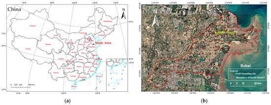
Figure 1.
(a,b) Location map of the study area and distribution map of sampling points.
The Kenli District features a typical deltaic topography, with the entire terrain sloping from the southwest toward the northeast estuary; it is overall flat, with a gradient of only 1/10,000 to 1/12,000. Due to sedimentation at different times and obstruction due to abandoned dams, complex micro-topographical forms such as hillocks and depressions are formed. Particularly, the terrain forms a slight slope towards the sea along the axis of the Yellow River, bulging into a fan facing the Bohai Sea, with an overall gradient of 1/8000. The Kenli District has two major soil types, tidal soil and saline soil, with the parent material being Yellow River alluvium due to the impact of the Yellow River. Due to the long-distance transport, sorting, and riverbed sedimentation of Yellow River silt, the majority of the delta’s particles are fine silt. Consequently, the soil texture in the Kenli District is relatively light, with sandy loam comprising 24.2% of the total region, light loam 46.1%, medium loam 14.8%, heavy loam 10.8%, and clay 4.8%, illustrating that sand and light loam are the most widely distributed, covering 70.3% of the total region.
2.2. Data Sources
2.2.1. Field Sampling
In this study, factors such as land use/cover types, elevation differences, and spatial accessibility were considered within the Kenli District to set up sampling points across the entire region and conduct field sampling. This paper takes into account seasonality and the growth period of the typical regional crop, winter wheat, specifically the two common irrigation periods (stem elongation and grain filling), as well as potential overpass times for remote sensing imagery in the region to select the sampling time. On a seasonal level, the year is divided into spring (March–May), summer (June–August), autumn (September–November), and winter (December–February). Spring is chosen to study soil salinity. For the winter wheat-growing period and its previous and subsequent irrigation phases, soil salinity is compared between the greening stage before irrigation and after the grain-filling stage post-irrigation. Combining the overlapping periods and planned overpass times of the imagery, the study confirmed extensive soil sampling in the study region from 29 May to 7 June 2022.
The field sampling method was based on conclusions drawn by Zhang Xiaoguang and others using geostatistical methods [30], noting that, due to the high variability in soil salinity in the Yellow River Delta, reducing the number of sampling points also reduces the ability to depict details; thus, a sufficient number of sampling points is essential to adequately express spatial heterogeneity. Therefore, this study, considering factors such as land use/cover types, elevation differences, and spatial accessibility, opted for a grid sampling method to set up comprehensive regional sampling. Sampling points were set up using a 5 km × 5 km-grid, uniform-layout method, with adjustments made to the actual positions as needed to ensure that the sampling points included various types of land use, such as farmland, forests, grasslands, and wastelands. Figure 1b illustrates the distribution map of field sampling points. To guarantee data accuracy, the sampling strategy involves a five-point sampling technique. This method collects soil samples from depths at 10-cm intervals, ranging from 0 to 10 cm and up to 90 to 100 cm. Additionally, each sampling location’s central coordinates are precisely documented using GPS to record the latitude and longitude. Due to surrounding construction or inaccessible regions, 83 sampling sites were selected, yielding a total of 819 effective samples.
2.2.2. Soil Analysis
Upon the return of the collected soil samples to the laboratory, the initial step involved the removal of larger solid particles or plant debris such as leaves and roots. Subsequently, the samples underwent a series of preparatory processes, which included air-drying, grinding, and sieving through a 2-mm mesh. The processed samples were then placed into new, self-sealing bags for subsequent analysis as test samples. The soil samples were utilized to determine the salt-content attributes. The procedure for assessing soil salinity is detailed as follows: soil samples, previously air-dried, ground, and sifted through a 2-mm sieve, were utilized to create a soil leachate using a water-to-soil ratio of 5:1. Specifically, 20 g of sieved samples were weighed and placed in a dry bottle, followed by the addition of 100 mL of distilled water using a graduated cylinder. The bottle was then tightly sealed and shaken in a shaker for 5 min before being left to stand for half an hour. The total salt content of the soil solution was determined using a portable multiparameter water-quality analyzer, specifically the HQ30d model from the calibrated Hach Company. The electrode head was immersed in the filtrate, and the measurement value was read after the numerical stability was achieved [31]. Some samples’ soil salinity data are shown in Table 1.

Table 1.
Partial sampling points data in Kenli District in May.
2.3. 3D-SSAS
The 3D-SSAS method process was as follows.
Construction of a 3D soil-voxel data set. At this step, the soil salinity sampling data were preprocessed using the 3D Empirical Bayesian Kriging (EBK) interpolation method to construct a 3D soil-voxel data set. The calculation of LAI: At this stage, the study proposed the definition of the Local Anomaly Index (LAI). LAI represents the degree of an anomaly in salinity at a central voxel relative to the surrounding voxels, with higher values indicating greater anomaly. Threshold selection and AV filtering: The input set for this step was the LAI collection obtained in the first step. A threshold was determined based on the distribution of the LAI collection, and voxels were divided into anomaly voxels (AVs) and normal voxels (NVs), with some AVs defined in this study as voxels that made up the anomalous-salinity area (ASA). Three-dimensional structure construction: This step was key to building the 3D structure of the ASA. In this step, the study used the 3D DBSCAN density-clustering algorithm, and by setting appropriate MinPts and Eps, it aggregated AVs into clusters, which formed the 3D structure of the ASA.
Figure 2 depicts the overall workflow of this study. The following section will elaborate on the four steps involved in the methodology.
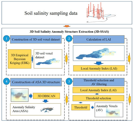
Figure 2.
Flow diagram of 3D-SSAS method.
2.3.1. Construction of 3D Soil-Salinity Voxel Data Set
This study was based on soil salinity-sampling data, using 3D EBK interpolation method to construct a data set as a 3D soil-voxel data set. Before using the 3D EBK interpolation method to expand the soil-salt space, the normal distribution of the interpolated data should be tested first. Only when the data obey the normal distribution can the Kriging method be used for interpolation. Descriptive statistical analysis of the samples was conducted using SPSS 22.0. The K-S test was employed to determine whether the data adhered to a normal distribution. For data that did not conform, a logarithmic transformation was applied to satisfy the normality criteria. After the preprocessing, the 3D EBK interpolation method was used to construct the 3D spatial data set of soil salinity of this study region, and the log-empirical method was selected by transforming type to realize the 3D spatial expansion of soil salinity in this region. The formula of 3D EBK is shown in Formula (1). Z(u) is the interpolation value at the target position u, n is the number of sample points, is the observation value at the i-th sample point, and is the interpolation weight, representing the contribution of sample point i to the target position u.
2.3.2. Calculation of Local Anomaly Index (LAI)
At the beginning of the method, this paper employs a voxel-by-voxel traversal, treating each voxel in the data set as a center voxel for the LAI calculation. LAI is a quantitative index used to measure an anomaly in soil salinity within the neighborhood of a voxel, quantifying the degree of a soil-salinity anomaly.
The study defined the concept of a “neighborhood” as illustrated in Figure 3. Consider the current center voxel denoted as v(x,y,z). A local coordinate system is established around the center voxel, v: the z-direction is the normal direction, with x and y directions perpendicular to z. In this coordinate system, a cube is established with v as the centroid and an edge length of 2dcartesian. We defined the neighborhood voxel set Nv of voxel v to be distributed on the 8 vertices and the midpoints of the 12 edges of the cube. In the three-dimensional coordinate system, there is a regular positional relationship between the central voxel, v, and its neighborhood voxel set, Nv. In this coordinate system, the coordinates of the center voxel, v, are (x, y, z), and its neighborhood voxel set, Nv, can be represented as follows: Nv = {x + ∆x, y + ∆y, z + ∆z: ∆x, ∆y, ∆z∈{0, dcartesian, −dcartesian}}. Based on the concept of a neighborhood, the calculation method for LAI is as follows:
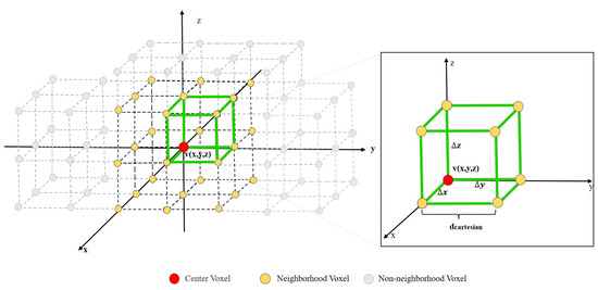
Figure 3.
The positional relationship between the center voxel and the neighborhood voxel.
The above formula I(x, y, z) represents the salinity value at the center voxel coordinates (x, y, z), I(xi, yi, zi) represents the salinity values at the coordinates (xi, yi, zi) of each voxel in the neighborhood voxel set, K represents the local variance between the center voxel and the neighborhood voxels, and δ represents the number of neighborhood voxels. Based on the above steps, the same calculations were performed for each voxel in the data set to obtain the LAI set for all voxels.
2.3.3. Threshold Selection and AV Filtering
After obtaining the LAI set, the study entered the threshold-selection phase, aimed at precisely determining the threshold through quantitative analysis. The setting of the threshold is key in distinguishing between AVs and NVs, requiring the calculation of voxels with the greatest change in magnitude based on the data set’s distribution characteristics.
Here is one method for selecting a threshold. First, the LAI set is processed into a collection, creating an LAI sequence, LS = {LAI(v1), LAI(v2), …, LAI(vn)}. This sequence is then sorted by value, forming an ascending sequence LS. The sorted LS is fitted to a curve, with the ordinate y as the LAI and the abscissa x as the index vi after sorting by LAI. Since vi are discrete points, the change in LAI should be calculated using the difference operation ΔLAI(vi) = LAI(vi+1) − LAI(vi). Given that the distribution of vi is equidistant, the first step should be to compute the first-order difference of LAI, ΔLAI(vi), to approximate the slope of LAI. Then, the second-order difference, Δ2 LAI(vi), should be calculated to further approximate the change in slope:
Then, all second-order differences, Δ2 LAI(vi), are iterated through to find the voxel with the maximum absolute value, which will be the threshold dthreshold.
The selection of AVs is based on the established threshold, dthreshold. Voxels with an LAI greater than the threshold are selected from all data voxels, they are identified as AVs, and they form the set .
2.3.4. Construction of 3D ASA Structure
This paper uses the 3D DBSCAN algorithm to construct AVs into a 3D structure of the anomalous-salinity area (ASA). A 3D DBSCAN, based on the neighborhood parameters Eps (radius of neighborhood) and MinPts (minimum number of neighborhood voxels within the eps radius), is used to quantify the internal compactness of data sample sets. Multiple neighborhood distance thresholds (Eps) were set for testing in the experiment, with the default minimum sample size threshold (MinPts) set to 10 and used for noise and small-region clustering to remove noise. The optimal clustering region was selected as the study region included in the scope of the research.
3. Results
3.1. Sampling Data Analysis
Table 2 presents statistical data on soil salinity across different layers, ranging from 0 to 100 cm in the study area. The salt content within this depth varied from 0.150 to 61.250 g/kg. The average salt concentration was 5.928 g/kg, with a median value of 2.900 g/kg and a coefficient of variation of 1.439. The highest salinity, reaching 61.250 g/kg, was observed in the surface layer (0–10 cm), displaying a logarithmic decrease from the surface downward. The overall average and median salinity values indicate substantial spatial variability, which was particularly pronounced within the plow layer (0–40 cm) and the deepest measured layer (90–100 cm).
Table 2.
Statistical characteristics of soil-salinity content in Kenli District for May.
3.2. Three-Dimensional Soil-Salinity Voxel Data Set
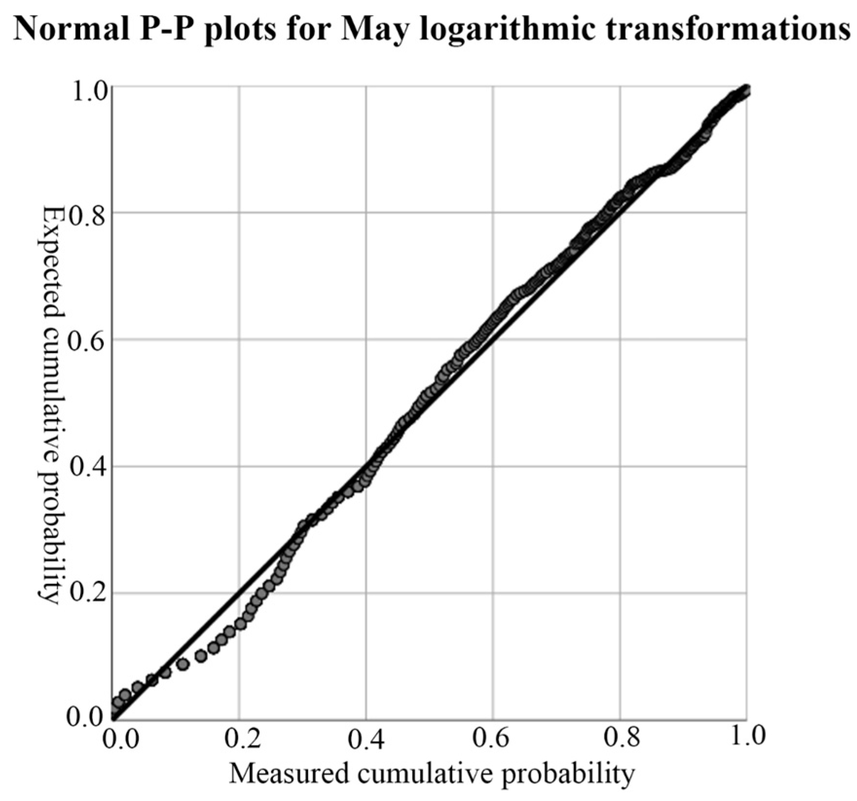
According to the results of the descriptive analysis in Table 2, both of the data were left-skewed, so they did not conform to the normal distribution. Therefore, a logarithmic transformation of the data was necessary to achieve a normal distribution. The P-P normal probability diagram was used to test the normal distribution results after conversion. If the data were normally distributed, the tested data would have basically formed a straight line, and the specific P-P normal probability diagram is shown in Figure 4. According to the results shown in Figure 4, the P-P normal probability chart, the tested data basically formed a straight line; that is, the data after the logarithmic conversion of soil-salt content presented the effect of normal distribution, and the Kriging method could be used for interpolation.

Figure 4.
Test for normal distribution of soil salinity in May. The black lines in the figure are 45° reference lines, and each gray dot represents a quantile in the data set.
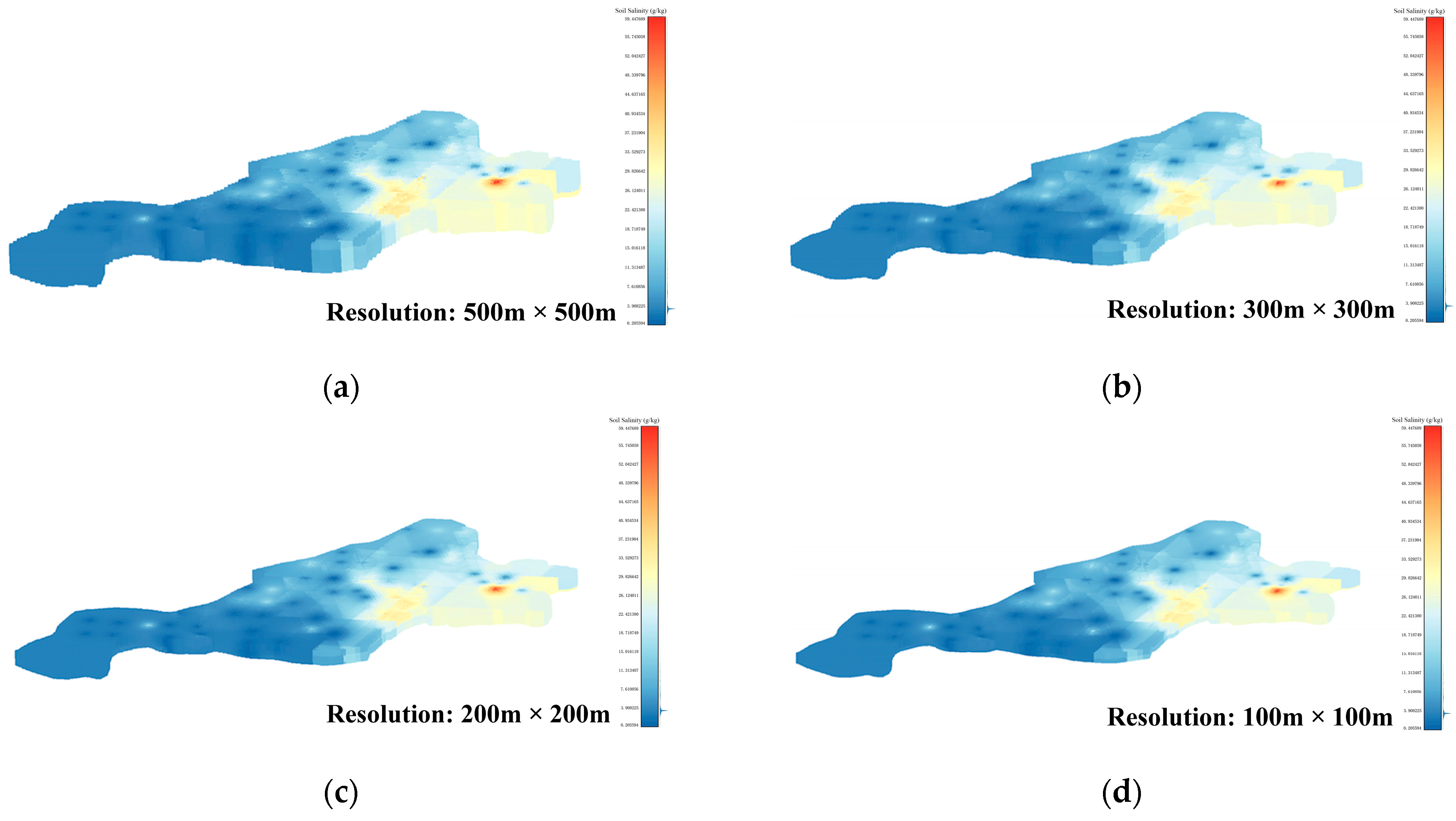
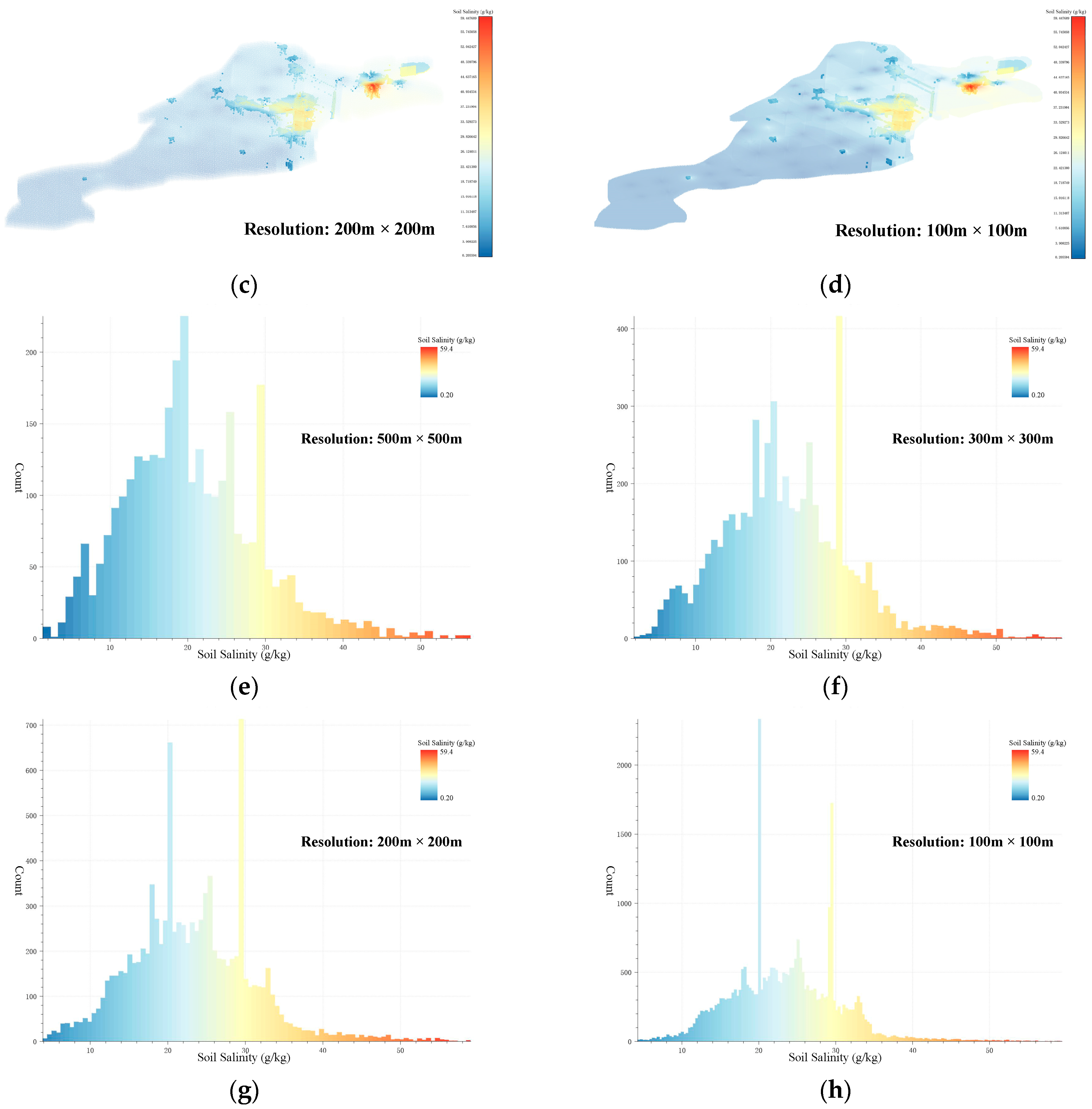
To ensure experimental accuracy, this paper thoroughly examines the limitations of the interpolation method and sets the resolution of the voxel data set to 500 m × 500 m, 300 m × 300 m, 200 m × 200 m, and 100 m × 100 m, respectively. The 3D-SSAS is applied to four distinct data sets, with the results subsequently compared. The data voxel sets of these four resolutions are shown in Figure 5a–d. The overall depth of each data set is 1 m, and it is divided into 10 layers; each layer is 10 cm apart.
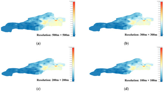
Figure 5.
Subfigures (a–d) show the 3D voxels of the soil-salinity distribution in the Kenli area at different resolutions: Subfigure (a) is from a 500 m × 500 m-resolution data set, subfigure (b) from a 300 m × 300 m-resolution data set, subfigure (c) from a 200 m × 200 m-resolution data set, and subfigure (d) from a 100 m × 100 m-resolution data set. The color variations in the figures indicate the levels of soil salinity.
3.3. Threshold and AV Sets
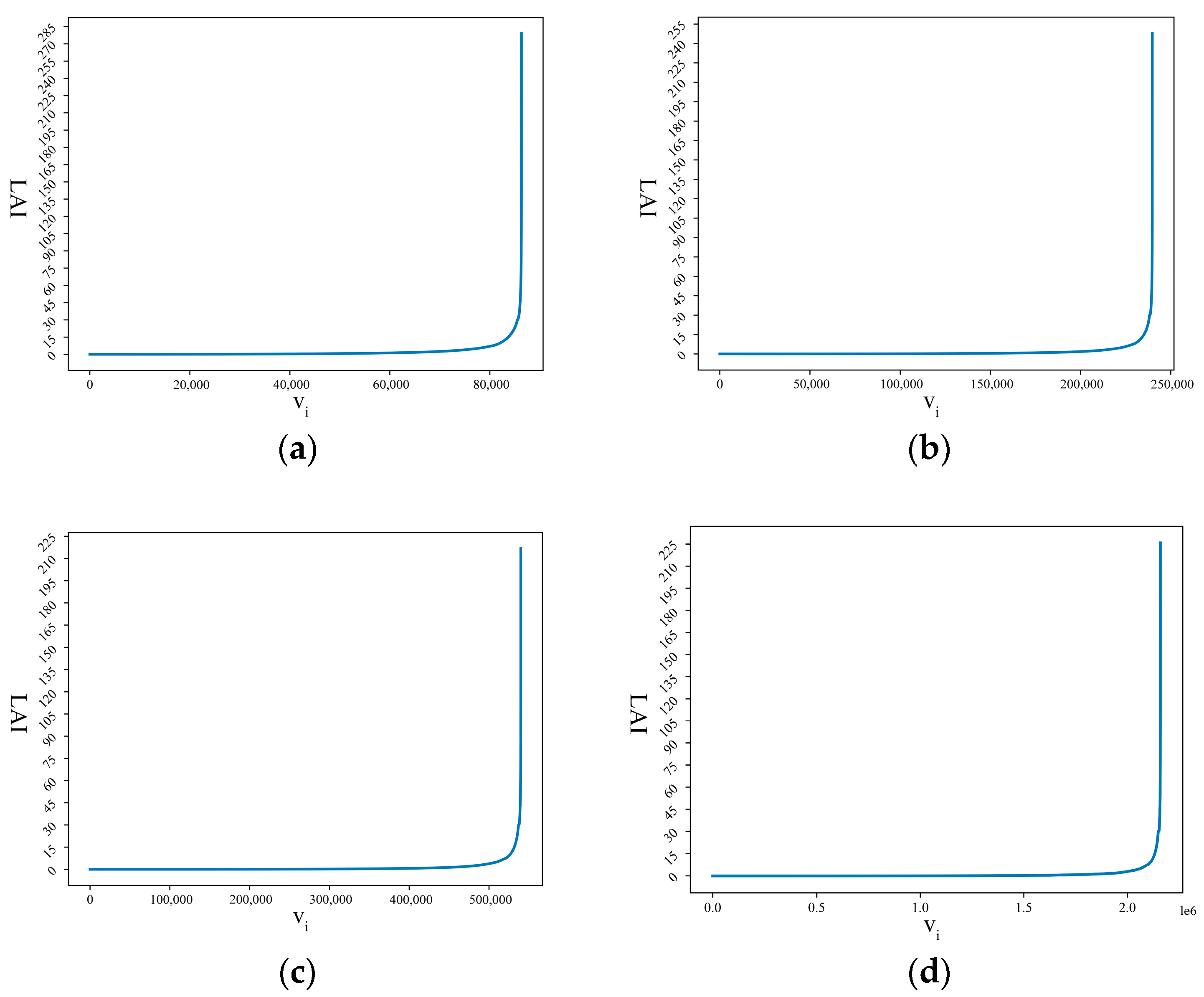
LAI calculation was performed on the above data sets; the sorted LAI sequences are described in Figure 6, and the graph shows the LS curves based on four different-resolution data sets. From the calculation process described in Section 2.3.3, the thresholds dthreshold for data sets of 500 m × 500 m, 300 m × 300 m, 200 m × 200 m, and 100 m × 100 m were 13.46, 13.33, 13.25, and 13.23, respectively.
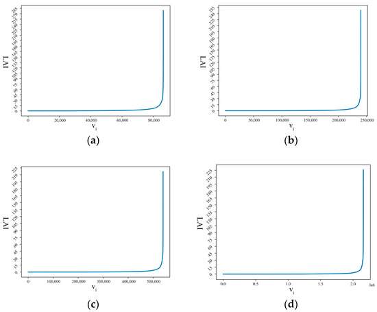
Figure 6.
Visualization of LS curves based on four different-resolution data sets. (a) LS curve at 500 m × 500 m resolution. (b) LS curve at 300 m × 300 m resolution. (c) LS curve at 200 m × 200 m resolution. (d) LS curve at 100 m × 100 m resolution.
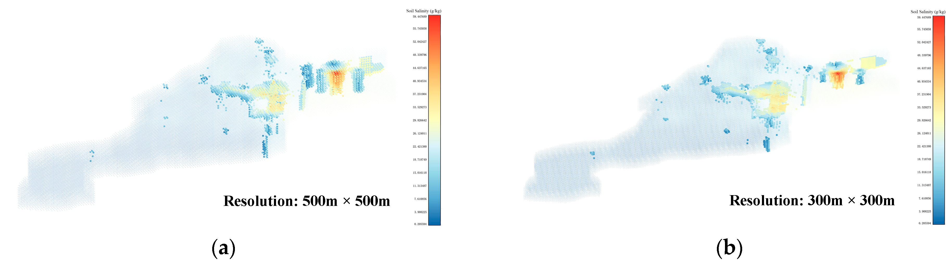
Using the threshold values obtained from the Threshold-selection step, the soil-salinity data at four different resolutions were subjected to AV filtering. The locations of the AV sets in the Kenli District soil-salinity data are shown in Figure 7a–d. The salinity distribution in the AV sets for the four resolutions is shown in Figure 7e–h. The number of AVs for the 500 m × 500 m resolution is 3142. For the 300 m × 300 m resolution, it was 5593. For the 200 m × 200 m resolution, it was 9808, and for the 100 m × 100 m resolution, it was 31,540. In the AV sets, the number of voxels with a salinity value of around 30 was the highest, followed by voxels with a salinity value of around 20. This phenomenon was more evident in the AV sets with resolutions of 200 m × 200 m and 100 m × 100 m. The voxel sets obtained from this step still contained some noisy voxels, which were difficult to form into regions. Denoising and clustering needed to be performed using 3D DBSCAN to construct the ASA 3D structure and obtain the final results of the 3D-SSAS.

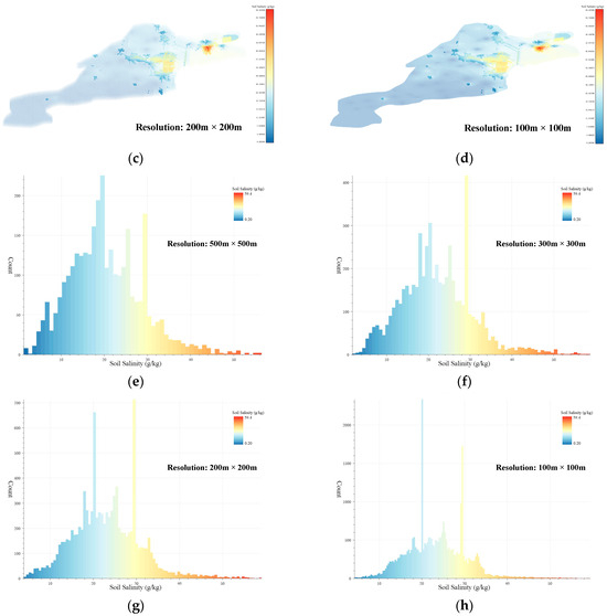
Figure 7.
Subfigures (a–d) show the locations of the AV sets in the Kenli soil-salinity data set in different-resolution data sets: Subfigure (a) is for the 500 m × 500 m-resolution data set, subfigure (b) for the 300 m × 300 m-resolution data set, subfigure (c) for the 200 m × 200 m-resolution data set, and subfigure (d) for the 100 m × 100 m-resolution data set. The colors in the figure represent the salinity content of the voxels. To better display the location of the AV sets, we made the other voxels transparent and enlarged the AVs for emphasis. Subfigures (e–h) are histograms of the salinity distribution for the AV sets at 500 m × 500 m, 300 m × 300 m, 200 m × 200 m, and 100 m × 100 m resolutions, where the colors represent the salinity content of the voxels.
3.4. Three-Dimensional Structure of ASA
This section presents the final results of the 3D-SSAS method. This study extracted three anomalous-salinity areas from soil-salinity data sets of the Yellow River Delta at four different resolutions (500 m × 500 m, 300 m × 300 m, 200 m × 200 m, and 100 m × 100 m). These regions display irregular 3D structures with a maximum depth of 1 m, as depicted in Figure 8.
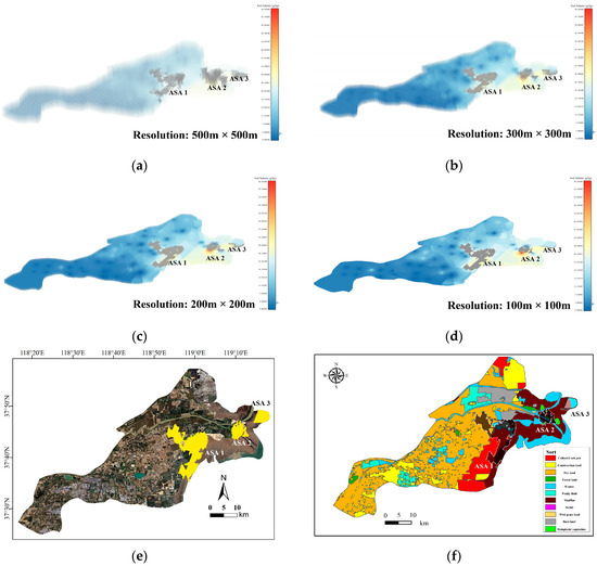
Figure 8.
Subfigures (a–d) visualize the extraction results of the 3D-SSAS method using data sets of different resolutions: Subfigure (a) for the 500 m × 500 m-resolution data set, subfigure (b) for the 300 m × 300 m-resolution data set, subfigure (c) for the 200 m × 200 m-resolution data set, and subfigure (d) for the 100 m × 100 m-resolution data set. The gray regions represent the ASAs. Due to the differences in resolution, there are subtle differences in the salinity distribution of each model. In order to better display ASA, the experiment shrinks the voxels of the data set during visualization. Figure (e) shows a two-dimensional image projection (yellow region) of the ASAs at a 100 m × 100 m resolution. Figure (f) shows the projection of ASAs on the land-use map. In the Figure, the black-shaded part is the structure shape of the ASA, and the white-shaded part is the underground shape.
Since the extraction results from data sets at the four resolutions are similar, to enhance model precision, this study selected the 100 m × 100 m-resolution salinity differentiated region for the main experimental results’ presentation. As shown in Figure 7e, the experiment detected three parts of soil salinity-differentiated regions in the Yellow River Delta region, located at the interface of the central woodland and salterns (ASA 1), the Yellow River estuary delta region (ASA 2), and the coastal region of the Kenli District in the east (ASA 3). As shown in Figure 8f, these regions are primarily located at the interfaces of different soil types. This section will present and explain the 3D structures of the ASAs, as illustrated in Figure 9, Figure 10 and Figure 11.
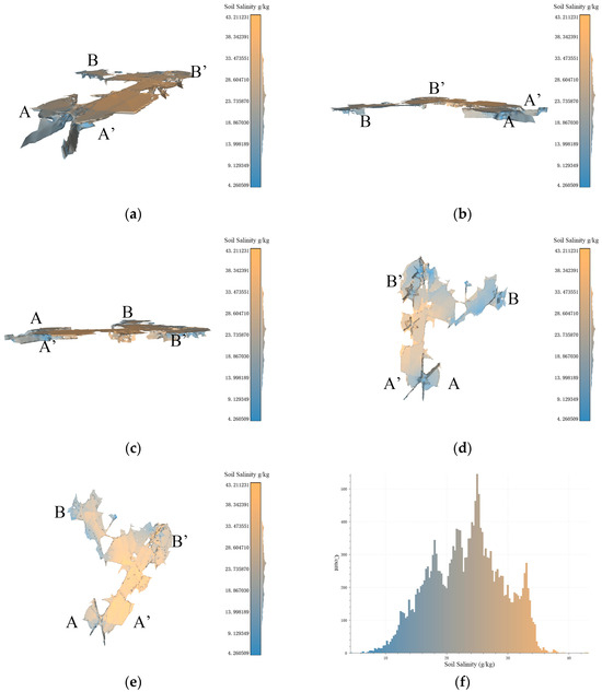
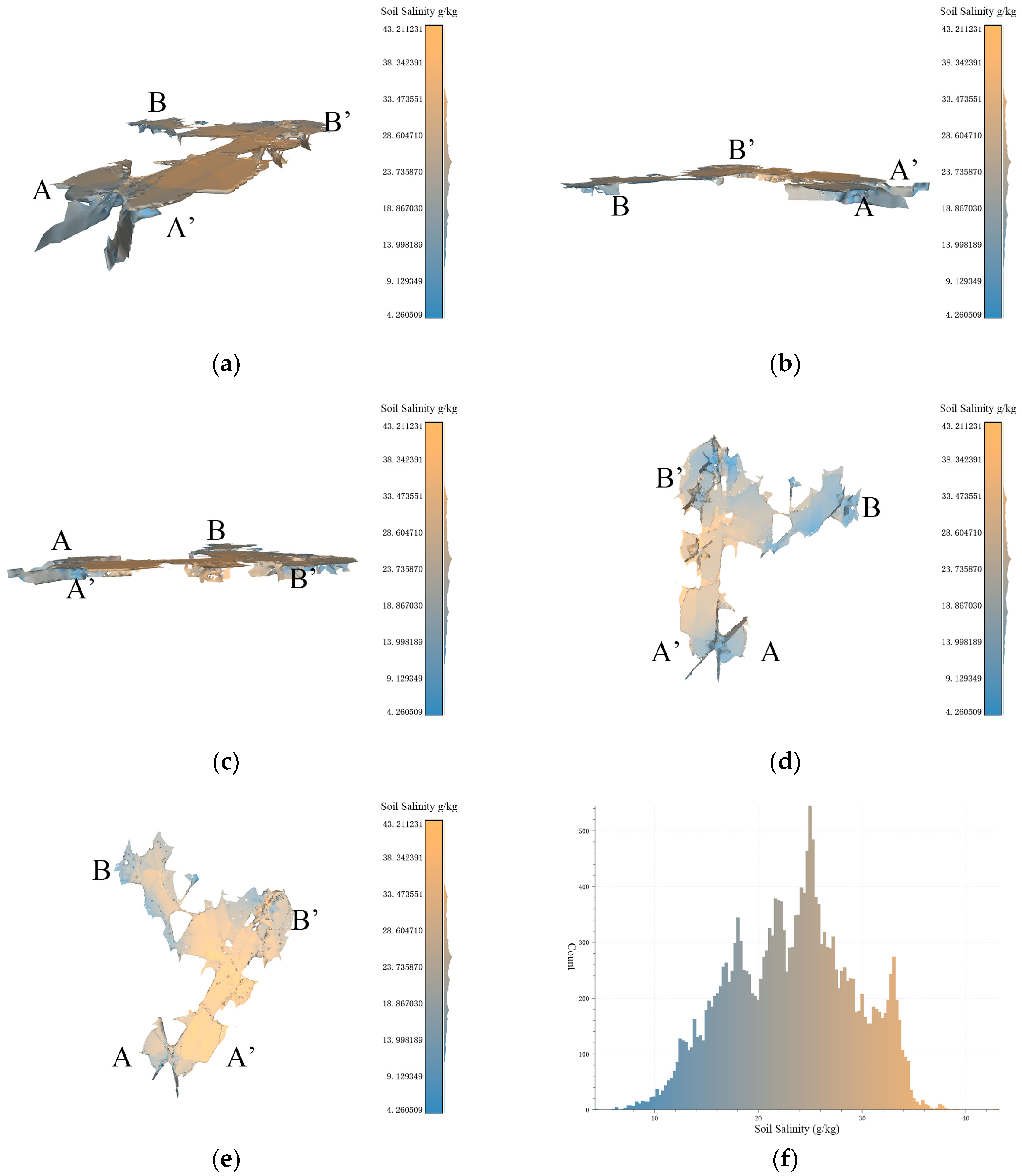
Figure 9.
Based on the data resolution of 100 m × 100 m, the experimental results of 3D-SSAS ASA1. In the Figure, A, A′, B, and B′ marks represent different angles of the model. (a) is the overall view of the model, (b,c) is the side view of the model, (d) is the bottom view, and (e) is the top view. (f) is the salt distribution map of ASA1.
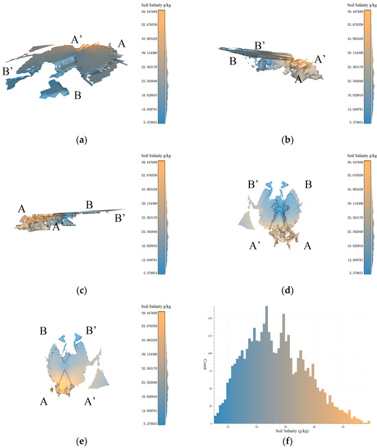
Figure 10.
Based on the data resolution of 100 m × 100 m, the experimental results of 3D-SSAS ASA2. In the Figure, A, A′, B, and B′ marks represent different angles of the model. (a) is the overall view of the model, (b,c) is the side view of the model, (d) is the bottom view, and (e) is the top view. (f) is the salt distribution map of ASA2.
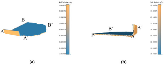
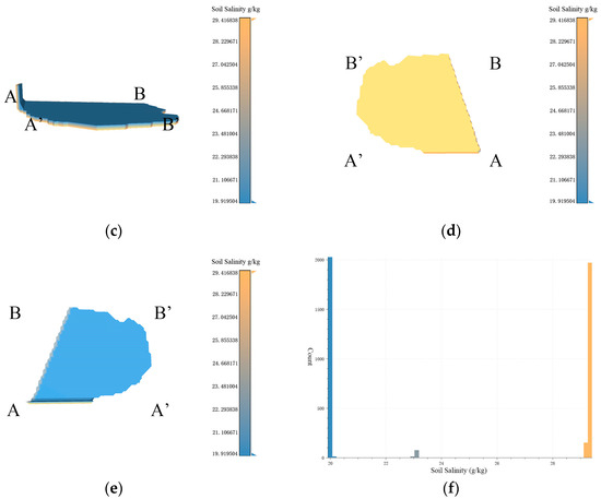
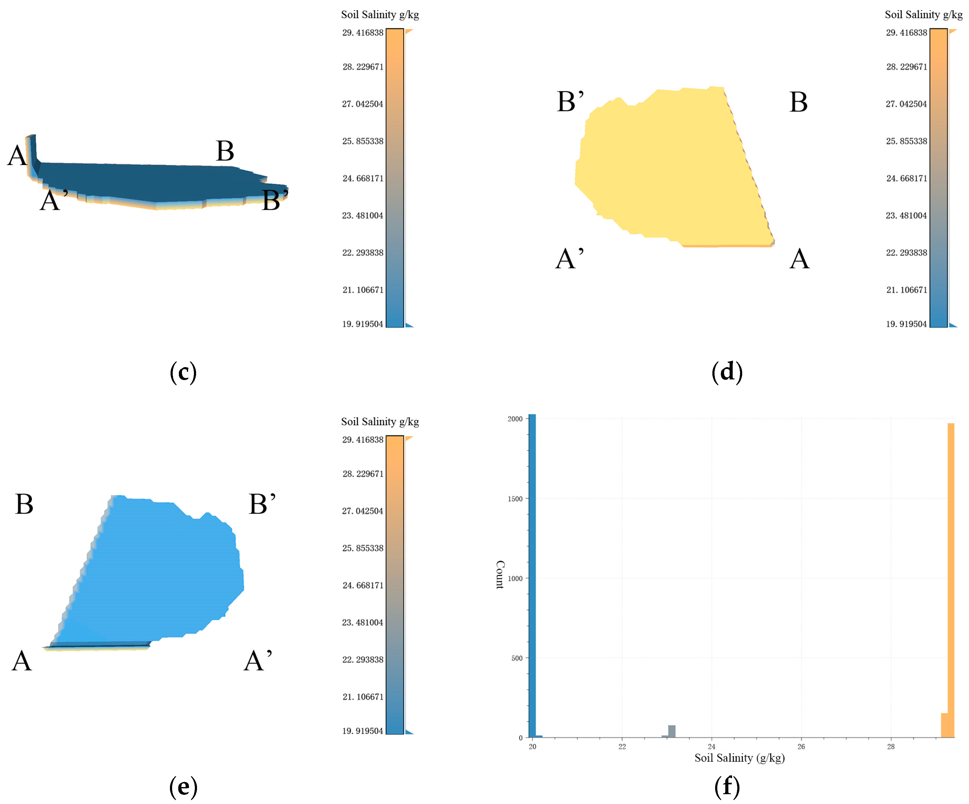
Figure 11.
Based on the data resolution of 100 m × 100 m, the experimental results of 3D-SSAS ASA3. In the Figure, A, A′, B, and B′ marks represent different angles of the model. (a) is the overall view of the model, (b,c) is the side view of the model, (d) is the bottom view, and (e) is the top view. (f) is the salt distribution map of ASA3.
3.4.1. ASA1
Figure 9a–f show a 3D model describing the 3D structure of the anomalous-salinity area 1 (ASA1) extracted via the algorithm described in this paper, primarily distributed along the Coastal Boulevard in the Kenli District, with central coordinates at 37°40′ N and 119°0′ E. According to the overhead view of the model in Figure 9e, ASA1 resembles the shape of the letter “C”, with the model primarily distributed at the structure and extending eastward from the central region and the end voxels extending north and south underground. Observations of the model’s bottom reveal several depressions at A, B, and B’, which, as seen from the side views in Figure 9b,c, extend down to 1 m below the ground. The ASA1 model shows a salinity pattern that is lower in the east and higher in the west, indicating a rising trend in soil salinity from the inland to coastal regions. As shown in Figure 8f, the model has a similar number of voxels on either side of the 24 g/kg boundary, marking it as an anomalous-salinity area.
The northeastern part of ASA1 exhibits an anomalous salinity gradient in the horizontal direction, as shown in Figure 9e, where the salinity increases from 6.5 g/kg to 38 g/kg from east to west. This is because the region is bisected by the Coastal Boulevard, which acts as a dike and alters the local soil-salinity characteristics [24]. In Figure 8f, the eastern land cover consists of tidal flats with high salinity, primarily due to their geographical location within the tidal zone, which leads to periodic submersion and exposure of the flats to seawater. As the tide recedes, soil moisture evaporates, leaving behind salt. The permeable soil allows seawater to penetrate more easily, bringing salt. Additionally, the seawater itself contains salt, and the presence of vegetation also affects salt concentration. These factors interact to make the tidal-flat soil rich in salt [32,33]. Compared to this, the salinity of the salt farms in the western part is lower, and this difference in salinity leads to the formation of a salinity-anomaly area here. The northwestern part of the region is influenced by waters connected to the sea, resulting in soil salinity that is higher than in surrounding regions and creating anomaly area features. Figure 9d shows multiple depressions in the bottom view of the model; these depressions were analyzed as sampling points.
3.4.2. ASA2
ASA2 (37°45′ N, 119°10′ E) spans between two tributaries at the mouth of the Yellow River, located near the Yuanwang Tower in the Yellow River Ecological Tourism Region. As shown in the overhead view in Figure 10e, the ASA2 model has a high middle and low sides from north to south, with scattered boundaries and a distinct flat region in the southeast, exhibiting an anomalous pattern of higher salinity in the south and lower in the north. The low-salinity parts occupy a larger proportion of this 3D space, with high-salinity regions only present in the south, tending below 0.5 m underground.
The northern part of ASA2 is similar in origin to ASA1, both being salinity-anomaly areas due to horizontal soil-salinity differences (Figure 10a), and both are located at the structure. However, the southern part of the model is located 0.5 m below the structure (Figure 10b,c), characterized by vertical scale differentiation. This region is a topographical depression and a convergence point for seawater, causing seawater to relatively stagnate at this location, facilitating the accumulation of salinity in the soil, and leading to increased salinity. Additionally, salt-tolerant vegetation such as Suaeda salsa, reeds, and Tamarix are distributed in this region. The uneven distribution of vegetation may lead to locally higher salt concentrations [34,35]. The salt content in samples from this region can be exceptionally high, reaching 59 g/kg. The pronounced variation in soil salinity across both horizontal and vertical dimensions significantly contributes to the formation of spatial ASA patterns in the surrounding region.
3.4.3. ASA3
ASA3 is primarily located 0.8 m to 0.9 m underground in the eastern coastal region of the Kenli District (37°48′ N, 119°19′ E), with a small part of its eastern region on the continental shelf. As shown in Figure 11a, its 3D form is a thin sheet structure with a thickness of 10 cm. According to Figure 11b, the northern section of the area extends into the structure, showing a consistent distribution of salinity across both the upper and lower layers of the model, marked by a noticeable salinity gradient. Figure 11f illustrates that the overall soil salinity distribution in the region is highly variable. A small section of the boundary region exhibits a salinity level of 23 g/kg, whereas other areas record salinity levels of 29.4 g/kg and 19.9 g/kg, respectively. As shown in Figure 8f, the land-use map, ASA3 includes a portion of water, which changes in size with the seasons. According to the data set, the sample points in the water during the sampling time are interpolated from the nearest neighboring terrestrial soil salinity, as described in Figure 11d, where the salinity in the water is the same as on land. Due to errors in the data set, we only analyzed the salinity properties of terrestrial soil.
According to Figure 11c, a salinity anomaly occurs at 0.8 m vertically in ASA3, which may be related to the stratification of soil salinity in tidal flats. In tidal-flat environments, due to factors like tides, soil salinity exhibits distinct vertical stratification. This phenomenon is quite common in tidal-flat ecosystems, and it involves the interplay of tides, hydrological conditions, soil characteristics, and vegetation [36,37].
4. Discussion
4.1. A Discussion of the 3D-SSAS Method
This study successfully applied the 3D-SSAS method to soil-salinity data in the Yellow River Delta, revealing in greater detail the 3D structures of anomalous-salinity areas (ASAs). Several key findings were made in the experiments: First, the algorithm showed significant consistency when processing data sets of different resolutions, confirming its robustness and reusability. Second, despite the prevalence of regular geometric structures in most soil-salinity grid samples from the Kenli District of the Yellow River Delta, some boundary regions, including coastal and administrative boundaries, displayed irregular shapes. The algorithm focuses solely on salinity differences between voxels without considering spatial relationships, yet it still achieves good extraction results. Third, the method successfully extracted 3D structures using 3D DBSCAN, effectively filtering out scattered noise voxels caused by original data errors. In terms of visualization, the algorithm is capable of observing the spatial variation in soil salinity in both horizontal and vertical dimensions, intuitively presenting the extracted ASA structure, such as the ASA3 region. This not only aids in a deeper understanding of the characteristics of an anomalous-salinity area but also provides researchers with a more intuitive tool to explain and communicate their findings.
However, it should be noted that the data set used is composed of sampled grid-point data, and the positional attributes must be representative. Although the study achieved results consistent with the spatial structure distribution of soil salinity in the research region and verified them through physical soil analysis, this does not necessarily guarantee absolute accuracy. Future work should consider using higher-precision data sets and explore the impact of interpolation methods on the accuracy of algorithmic extraction.
4.2. Ecological, Agricultural, and Environmental Impacts
In this study, the impact of ASAs on vegetation distribution was investigated. The results indicate that, in regions with a higher LAI, such as ASA2, the structure and composition of vegetation communities have significantly changed [38]. The dominance of salt-tolerant plants significantly increases in high-salinity regions, while the dominance of non-salt-tolerant plants may be suppressed [39,40,41]. Furthermore, we discovered that ASAs affect the seasonality and spatiotemporal dynamics of vegetation growth, which has profound implications for species diversity and the ecological functions of ecosystems [42,43,44,45,46]. To better understand the adaptation mechanisms of vegetation to soil-salinity heterogeneity, future research could reveal these response mechanisms at the physiological and molecular biology levels.
In agriculture, ASAs significantly affect crop growth conditions [47]. Research has found that the soil-salinity structure in the ASA2 region is closely related to crop adaptability, with some crops showing greater resistance in high-salinity regions, such as Tamarix and Rheum. However, in the northern part of ASA1, according to its 3D model, the salinity anomaly extends down to 1 m underground, where crop growth may be limited by soil-salinity heterogeneity, leading to decreased productivity [48]. Therefore, formulating reasonable land-use planning is key to promoting sustainable development in the Yellow River Delta region. Based on our research findings, we recommend dividing the land into different management regions based on the 3D distribution of salinity while considering various factors such as soil-salinity structure, vegetation distribution, and human activities [49,50,51].
5. Conclusions
The study proposed an innovative and effective method 3D-SSAS for extracting the 3D structure of an anomalous-salinity area (ASA). The main conclusions are as follows: First, we successfully developed a method that integrates spatial soil characteristics and salinity-anomaly changes, fully exploring the structure of a soil-salinity anomaly area. This method is not limited to two-dimensional planes but also analyzes salt data in 3D space, more accurately reflecting complex changes in soil salinity. Second, experiments conducted with field-collected soil-salinity data sets verified the performance of the method. This study selected the typical coastal saline–alkaline region of the Yellow River Delta, the Kenli District, as the research region. Through field sampling, vertically stratified soil-salinity data were obtained. The results show that the ASA regions identified using the method are significantly accurate and authentic in terms of causality, proving the effectiveness and feasibility of the method in regional soil-salinity structure monitoring. Furthermore, our method adaptively adjusts threshold parameters according to different data, accommodating changes across different temporal and spatial scales and thereby facilitating ASA extraction under various salinity levels, from seasonal changes to rapid responses to sudden events.
However, this study also faced some limitations. Firstly, the quality of data and interpolation methods can affect the outcome of the method; secondly, the choice of threshold values may have overlooked some ASAs that are still of research significance. In summary, this method provides a novel and effective approach to the detection and analysis of a salinity anomaly. Future research could further extend this method’s application to other soil-attribute variables, handle more types of soil data, further explore the relationship between soil-variable differences and environmental changes, and make a more profound contribution to soil science and environmental research.
Author Contributions
Conceptualization, Z.H., X.F. and H.Z.; Methodology, Z.H., J.Y. and H.Z.; Software, Z.H.; Validation, Z.H.; Formal analysis, J.Y.; Data curation, J.Y.; Writing—original draft, Z.H.; Writing—review & editing, Z.H., X.F. and H.Z.; Supervision, X.F.; Project administration, X.F. All authors have read and agreed to the published version of the manuscript.
Funding
This work was supported by the National Key Research and Development Program of China [grant number 2022YFB3904102], the Innovation Project of LREIS [grant number 08R8A092YA] and the Shandong Provincial Natural Science Foundation [grant number ZR2022MD059].
Data Availability Statement
The original contributions presented in the study are included in the article, further inquiries can be directed to the corresponding author.
Acknowledgments
We thank the anonymous referees for their helpful and insightful comments and suggestions on this manuscript.
Conflicts of Interest
The authors declare no conflicts of interest.
References
- Dehaan, R.; Taylor, G. Field-derived spectra of salinized soils and vegetation as indicators of irrigation-induced soil salinization. Remote Sens. Environ. 2002, 80, 406–417. [Google Scholar] [CrossRef]
- Li, J.; Pu, L.; Han, M.; Zhu, M.; Zhang, R.; Xiang, Y. Soil salinization research in China: Advances and prospects. J. Geogr. Sci. 2014, 24, 943–960. [Google Scholar] [CrossRef]
- Wang, X.P.; Yang, J.S.; Liu, G.M.; Yao, R.J.; Yu, S.P. Impact of irrigation volume and water salinity on winter wheat productivity and soil salinity distribution. Agric. Water Manag. 2015, 149, 44–54. [Google Scholar] [CrossRef]
- Machado, R.M.A.; Serralheiro, R.P. Soil salinity: Effect on vegetable crop growth. Management practices to prevent and mitigate soil salinization. Horticulturae 2017, 3, 30. [Google Scholar] [CrossRef]
- Pessoa, L.G.M.; Freire, M.B.G.d.S.; Green, C.H.M.; Miranda, M.F.A.; Filho, J.C.d.A.; Pessoa, W.R.L.S. Assessment of soil salinity status under different land-use conditions in the semiarid region of Northeastern Brazil. Ecol. Indic. 2022, 141, 109139. [Google Scholar] [CrossRef]
- Gong, L.; Ran, Q.; He, G.; Tiyip, T. A soil quality assessment under different land use types in Keriya river basin, Southern Xinjiang, China. Soil Tillage Res. 2015, 146, 223–229. [Google Scholar] [CrossRef]
- Akça, E.; Aydin, M.; Kapur, S.; Kume, T.; Nagano, T.; Watanabe, T.; Çilek, A.; Zorlu, K. Long-term monitoring of soil salinity in a semi-arid environment of Turkey. Catena 2020, 193, 104614. [Google Scholar] [CrossRef]
- Onkware, A.O. Effect of soil salinity on plant distribution and production at Loburu delta, Lake Bogoria National Reserve, Kenya. Austral Ecol. 2000, 25, 140–149. [Google Scholar] [CrossRef]
- Fereres, E.; Soriano, M.A. Deficit irrigation for reducing agricultural water use. J. Exp. Bot. 2007, 58, 147–159. [Google Scholar] [CrossRef]
- Bekmirzaev, G.; Ouddane, B.; Beltrao, J.; Khamidov, M.; Fujii, Y.; Sugiyama, A. Effects of Salinity on the Macro- and Micronutrient Contents of a Halophytic Plant Species (Portulaca oleracea L.). Land 2021, 10, 481. [Google Scholar] [CrossRef]
- Li, X.; Guo, M. The Impact of Salinization and Wind Erosion on the Texture of Surface Soils: An Investigation of Paired Samples from Soils with and without Salt Crust. Land 2022, 11, 999. [Google Scholar] [CrossRef]
- Yang, W.; Song, X.; He, Y.; Chen, B.; Zhou, Y.; Chen, J. Distribution of Soil Organic Carbon Density Fractions in Aggregates as Influenced by Salts and Microbial Community. Land 2023, 12, 2024. [Google Scholar] [CrossRef]
- Jordán, M.; Navarro-Pedreno, J.; García-Sánchez, E.; Mateu, J.; Juan, P. Spatial dynamics of soil salinity under arid and semi-arid conditions: Geological and environmental implications. Environ. Geol. 2004, 45, 448–456. [Google Scholar] [CrossRef]
- Zhang, Y.; Miao, Q.; Li, R.; Sun, M.; Yang, X.; Wang, W.; Huang, Y.; Feng, W. Distribution and Variation of Soil Water and Salt before and after Autumn Irrigation. Land 2024, 13, 773. [Google Scholar] [CrossRef]
- Akramkhanov, A.; Martius, C.; Park, S.; Hendrickx, J. Environmental factors of spatial distribution of soil salinity on flat irrigated terrain. Geoderma 2011, 163, 55–62. [Google Scholar] [CrossRef]
- Bannari, A.; Abuelgasim, A. Potential and limits of vegetation indices compared to evaporite mineral indices for soil salinity discrimination and mapping. SOIL Discuss. 2021, 2021, 1–48. [Google Scholar]
- Wang, Y.; Deng, C.; Liu, Y.; Niu, Z.; Li, Y. Identifying change in spatial accumulation of soil salinity in an inland river watershed, China. Sci. Total Environ. 2018, 621, 177–185. [Google Scholar] [CrossRef]
- Wang, F.; Shi, Z.; Biswas, A.; Yang, S.; Ding, J. Multi-algorithm comparison for predicting soil salinity. Geoderma 2020, 365, 114211. [Google Scholar] [CrossRef]
- Naimi, S.; Ayoubi, S.; Zeraatpisheh, M.; Dematte, J.A.M. Ground observations and environmental covariates integration for mapping of soil salinity: A machine learning-based approach. Remote Sens. 2021, 13, 4825. [Google Scholar] [CrossRef]
- Gu, Q.; Han, Y.; Xu, Y.; Ge, H.; Li, X. Extraction of saline soil distributions using different salinity indices and deep neural networks. Remote Sens. 2022, 14, 4647. [Google Scholar] [CrossRef]
- Peng, J.; Biswas, A.; Jiang, Q.; Zhao, R.; Hu, J.; Hu, B.; Shi, Z. Estimating soil salinity from remote sensing and terrain data in southern Xinjiang Province, China. Geoderma 2019, 337, 1309–1319. [Google Scholar] [CrossRef]
- Wang, N.; Xue, J.; Peng, J.; Biswas, A.; He, Y.; Shi, Z. Integrating remote sensing and landscape characteristics to estimate soil salinity using machine learning methods: A case study from Southern Xinjiang, China. Remote Sens. 2020, 12, 4118. [Google Scholar] [CrossRef]
- Zovko, M.; Romić, D.; Colombo, C.; Di Iorio, E.; Romić, M.; Buttafuoco, G.; Castrignanò, A. A geostatistical Vis-NIR spectroscopy index to assess the incipient soil salinization in the Neretva River valley, Croatia. Geoderma 2018, 332, 60–72. [Google Scholar] [CrossRef]
- Fu, X.; Liu, G.; Huang, C.; Liu, Q. Analysis of ecological characteristics of coastal zone in Yellow River Delta under dam disturbance. J. Geo-Inform. Sci. 2011, 13, 797–803. [Google Scholar] [CrossRef]
- Singh, A. Soil salinization management for sustainable development: A review. J. Environ. Manag. 2021, 277, 111383. [Google Scholar] [CrossRef]
- Zhang, H.; Fu, X.; Zhang, Y.; Qi, Z.; Zhang, H.; Xu, Z. Mapping Multi-Depth Soil Salinity Using Remote Sensing-Enabled Machine Learning in the Yellow River Delta, China. Remote Sens. 2023, 15, 5640. [Google Scholar] [CrossRef]
- Guan, Y.; Liu, G.; Wang, J. Regionalization of Salt-affected Land for Amelioration in the Yellow River Delta Based on GIS. Acta Geogr. Sin. 2001, 56, 205–212. [Google Scholar]
- De Sosa, L.L.; Martin-Palomo, M.J.; Castro-Valdecantos, P.; Madejon, E. Agricultural use of compost under different irrigation strategies in a hedgerow olive grove under Mediterranean conditions—A comparison with traditional systems. Soil 2023, 9, 325–338. [Google Scholar] [CrossRef]
- Chen, H.; Liang, M.; Liu, W.; Wang, W.; Liu, P.X. An approach to boundary detection for 3D point clouds based on DBSCAN clustering. Pattern Recognit. 2022, 124, 108431. [Google Scholar] [CrossRef]
- Zhang, X.; Wang, Z.; Song, X.; Liu, P.; Li, S.; Yang, X. Effect of sampling on spatial variability in soil salinity in the Yellow River Delta Area. Resour. Sci. 2016, 12, 2375–2382. [Google Scholar]
- Fan, X.; Pedroli, B.; Liu, G.; Liu, Q.; Liu, H.; Shu, L. Soil salinity development in the yellow river delta in relation to groundwater dynamics. Land Degrad. Dev. 2012, 23, 175–189. [Google Scholar] [CrossRef]
- Gulzar, S.; Khan, M.A.; Ungar, I.A. Salt tolerance of a coastal salt marsh grass. Commun. Soil Sci. Plant Anal. 2003, 34, 2595–2605. [Google Scholar] [CrossRef]
- Yang, L.; Yan, C.X.; Ni, L.H.; Ting, L.T.; Jun, G.; Qiang, F.U. Relationships between Salinity, Conductivity and Water Content of Soils in a Pristine Tidal Flat in Jiangsu Province. Water Sav. Irrig. 2015, 8, 4–7. [Google Scholar]
- Qin, Z.J.; Bo, C.J.; Guang, Y.C.; Gui, G.A.; Xiu, L.J.; Long, Y.Y. Growth adaptability of some cultivars(lines) of warm-season turfgrass in coastal beach and their influence on soil salinity. J. Plant Resour. Environ. 2010, 19, 48–54. [Google Scholar]
- Ce, Y.; Huanyu, C.; Jinsong, L.I.; Yu, T.; Xiaohui, F.; Xiaojing, L.; Kai, G. Soil improving effect of Suaeda salsa on heavy coastal saline-alkaline land. Chin. J. Eco-Agric. 2019, 27, 1578–1586. [Google Scholar]
- Fan, X.; Liu, G.; Tang, Z.; Shu, L. Analysis on main contributors influencing soil salinization of Yellow River Delta. J. Soil Water Conserv. 2010, 24, 139–144. [Google Scholar]
- Qing, W.; Meng, L.; Dong-Dong, Q.; Tian, X.; Wei, S.; Bao-Shan, C.; Environment, S.O.; University, B.N. Effect of hydrological characteristics on the recruitment of Suaeda salsa in coastal salt marshes. J. Nat. Resour. 2019, 34, 2569–2579. [Google Scholar] [CrossRef]
- Wang, Z.; Zhao, G.; Gao, M.; Chang, C. Spatial variability of soil salinity in coastal saline soil at different scales in the Yellow River Delta, China. Environ. Monit. Assess. 2017, 189, 80. [Google Scholar] [CrossRef]
- Bazihizina, N.; Barrett-Lennard, E.G.; Colmer, T.D. Plant growth and physiology under heterogeneous salinity. Plant Soil 2012, 354, 1–19. [Google Scholar] [CrossRef]
- Valenzuela, F.J.; Reineke, D.; Leventini, D.; Chen, C.C.L.; Barrett-Lennard, E.G.; Colmer, T.D.; Dodd, I.C.; Shabala, S.; Brown, P.; Bazihizina, N. Plant responses to heterogeneous salinity: Agronomic relevance and research priorities. Ann. Bot. 2022, 129, 499–518. [Google Scholar] [CrossRef]
- Reynolds, H.L.; Hungate, B.A.; Chapin Iii, F.; D’Antonio, C.M. Soil heterogeneity and plant competition in an annual grassland. Ecology 1997, 78, 2076–2090. [Google Scholar] [CrossRef]
- Moffett, K.B.; Robinson, D.A.; Gorelick, S.M. Relationship of salt marsh vegetation zonation to spatial patterns in soil moisture, salinity, and topography. Ecosystems 2010, 13, 1287–1302. [Google Scholar] [CrossRef]
- Liu, L.; Wu, Y.; Yin, M.; Ma, X.; Yu, X.; Guo, X.; Du, N.; Eller, F.; Guo, W. Soil salinity, not plant genotype or geographical distance, shapes soil microbial community of a reed wetland at a fine scale in the Yellow River Delta. Sci. Total Environ. 2023, 856, 159136. [Google Scholar] [CrossRef] [PubMed]
- Gilliam, F.S.; Dick, D.A. Spatial heterogeneity of soil nutrients and plant species in herb-dominated communities of contrasting land use. Plant Ecol. 2010, 209, 83–94. [Google Scholar] [CrossRef]
- Zhao, S.; Liu, J.J.; Banerjee, S.; White, J.F.; Zhou, N.; Zhao, Z.Y.; Zhang, K.; Hu, M.F.; Kingsley, K.; Tian, C.Y. Not by salinity alone: How environmental factors shape fungal communities in saline soils. Soil Sci. Soc. Am. J. 2019, 83, 1387–1398. [Google Scholar] [CrossRef]
- Li, Y.; Kang, E.; Song, B.; Wang, J.; Zhang, X.; Wang, J.; Li, M.; Yan, L.; Yan, Z.; Zhang, K. Soil salinity and nutrients availability drive patterns in bacterial community and diversity along succession gradient in the Yellow River Delta. Estuar. Coast. Shelf Sci. 2021, 262, 107621. [Google Scholar] [CrossRef]
- Adamchuk, V.I.; Ferguson, R.B.; Hergert, G.W. Soil heterogeneity and crop growth. In Precision Crop Protection—The Challenge and Use of Heterogeneity; Springer: Berlin/Heidelberg, Germany, 2010; pp. 3–16. [Google Scholar]
- Wang, Y.; Liu, G.; Zhao, Z. Spatial heterogeneity of soil fertility in coastal zones: A case study of the Yellow River Delta, China. J. Soils Sediments 2021, 21, 1826–1839. [Google Scholar] [CrossRef]
- Russo, D. A stochastic approach to the crop yield-irrigation relationships in heterogeneous soils: I. Analysis of the field spatial variability. Soil Sci. Soc. Am. J. 1986, 50, 736–745. [Google Scholar] [CrossRef]
- Patzold, S.; Mertens, F.M.; Bornemann, L.; Koleczek, B.; Franke, J.; Feilhauer, H.; Welp, G. Soil heterogeneity at the field scale: A challenge for precision crop protection. Precis. Agric. 2008, 9, 367–390. [Google Scholar] [CrossRef]
- Liu, Y.; Ma, C.; Yang, Z.; Fan, X. Ecological Security of Desert–Oasis Areas in the Yellow River Basin, China. Land 2023, 12, 2080. [Google Scholar] [CrossRef]


Disclaimer/Publisher’s Note: The statements, opinions and data contained in all publications are solely those of the individual author(s) and contributor(s) and not of MDPI and/or the editor(s). MDPI and/or the editor(s) disclaim responsibility for any injury to people or property resulting from any ideas, methods, instructions or products referred to in the content. |
© 2024 by the authors. Licensee MDPI, Basel, Switzerland. This article is an open access article distributed under the terms and conditions of the Creative Commons Attribution (CC BY) license (https://creativecommons.org/licenses/by/4.0/).