Abstract
The Ili River Basin (IRB) is located in the northwest of China. With its large-scale zone and abundant resources, it is believed to be a “wet island” and a biotic resource storehouse in the dry regions of Eurasia. The IRB has stable ecological conditions and abundant water resources, providing natural conditions for agricultural production and human settlements. With the population increasing and economic development advancing, the competition for land resources is becoming fierce, leading to some ecological problems in this region. Therefore, understanding the spatiotemporal changes and driving mechanisms of the “three-zone space” (TZS) in the IRB is of significant practical importance for promoting sustainable development and optimizing the territorial spatial pattern. This study first analyzes the characteristics and intensity of the TZS changes from 2000 to 2020. Then, it utilizes the optimized parameter Geodetector (OPGD) to analyze the driving mechanisms behind these changes. The results show the following. Firstly, the agricultural space (AS) increased by a total of 837.5 km2, the urban space (US) increased by 519.64 km2, and other ecological space (OES) increased by 1518.83 km2. Green ecological space (GES) decreased by 2875.97 km2. Secondly, intensity analysis indicated that the total TZS change in IRB was 11.07%. At the spatial-type level, the increased intensities of OES, US, and AS were active. In spatial transformation intensity, US and OES tended to transform into AS; AS tended to transform into US; and OES and GES had a mutual transformation tendency. Thirdly, AS converted into US around emerging cities like Khorgas and Cocodala. The conversion towards GES was scattered. The mutual conversion between OES and GES showed spatial distribution consistency, mainly occurring in the Borohoro ranges and the Halik ranges. Lastly, regarding the driving mechanisms, the evolution of US in the IRB was driven by social and economic factors. Location and climate factors accelerated agricultural development, facilitating the transformation of GES and OES into AS. Climate and economic factors played a crucial role in the scale of conversions between OES and GES. The findings can provide a basis for the governance and protection of the IRB, help to form a rational territorial spatial pattern, and offer scientific guidance for sustainable land management.
1. Introduction
The Sustainable Development Goals (SDGs) were released by the United Nations in September 2015 [1]. The SDGs aim to serve as a guide for nations in shaping their planning, policy, and investment strategies, as well as in consistently monitoring and reporting their advancements towards sustainable development from 2016 to 2030 [2]. China actively engages in global environmental and climate governance.
Territorial space is essential for human survival and development; it is a crucial resource for sustainable societal progress and national power [3,4,5]. China has achieved significant advancements in both its economic and social progress, with accelerated territorial space development in these years. However, issues, such as disorder of spatial development, inefficient resource use, and shrinking ecological space, have emerged [6,7,8]. Thus, to achieve the SDGs, China has advocated for the establishment of a “Three Zones and Three Lines” framework [9] to create an integrated spatial management system. This framework categorizes territorial space into urban, agricultural, and ecological spaces, each demarcated by the following distinct control lines: the urban development boundary, the boundary for permanent agricultural land, and the ecological protection red line, respectively. The changes in ecological space, agricultural space, and urban space reflect the extent of the influence of human activities [10]. It plays a crucial bridging role between the macro scale (major function-oriented zone [11]) and the micro scale (land use planning [9]). Despite differences in land classification systems and spatial dominant functions, the “three-zone space” (TZS) classification is more suitable for medium to large-scale analyses [12].
The scope of this study is the Ili River Basin (IRB) within China. The Ili River is shared by both China (approximately 624 km long, upstream) and Kazakhstan (approximately 815 km long, downstream) [13,14], with several originated branch rivers including the Tekes River, Kash River, and Gongnaisi River. The IRB, situated in the western part of the Xinjiang Uygur Autonomous Region (XUAR) in Central Asia, is a crucial sensitive ecological environment zone in China [15], and it is known as “Jiangnan beyond the Great Wall”. Additionally, it features three border trade ports, namely, Khorgos, Dulata, and Muzhaerte, of which Khorgos stands out as a crucial hub for the New Eurasian Land Bridge, making it the largest land port between China and Kazakhstan [16]. In recent years, the Ili Kazakh Autonomous Prefecture government has introduced and revised the “Ili River Valley Ecological Environment Protection Regulations”, formulated the “14th Five-Year Plan for Ecological Environment Protection”, and implemented the “Three Lines One Permit” policy [17,18]. These initiatives were designed to regulate the protection of the ecological environment, taking into account factors like industrial scale, spatial distribution, environmental risk mitigation, and ecological carrying capacity, with the goal of achieving a balanced relationship between human activities and the natural world.
With the implementation of the Western Development strategy [19] and socio-economic improvements, the rapid expansion of urban space in the IRB has encroached on ecological and agricultural space, leading to conflicts between development and protection as well as tensions in the relationship between humans and land. To mitigate these issues, it is essential to construct a rationally structured and spatially ordered pattern based on the TZS framework. Specifically, it is crucial to describe the trends and intensities of changes occurring within urban, ecological, and agricultural spaces. By analyzing the distribution, kernel density, and spatial exchange intensity of the TZS from 2000 to 2020, we can determine the scale, intensity, and patterns of the spatial changes in the TZS. This work will help optimize the territorial spatial pattern. The use of a space pattern transfer matrix [20], kernel density estimation [21], and TZS dynamic degree [11] methods is suitable for achieving this goal. Current research on the IRB primarily focuses on the sources of soil and potential distribution mechanisms [22,23,24], the distribution and impact mechanisms of diseases [25], and areas such as hydrology [26], the ecological environment [27], and climate [28,29]. There is limited research on land use [30,31] and a lack of studies on the evolution processes and impact mechanisms of the TZS in the IRB from the perspective of territorial spatial planning. The transition matrix is a fundamental method in the analysis of land change [32]. To explain the changes in the TZS, one can utilize the land use transition matrix method to obtain accurate information about the potential processes that drive the changes. Intensity analysis is a hierarchical analysis method used to analyze land use change in terms of its interval, category, and transition level [33,34,35]. This study utilizes intensity analysis to assess the magnitude and intensity of total losses and gains for each spatial type at the category level between 2000 and 2020. At the transition level, it analyzes the size and intensity of specific spatial types transitioning to other categories between 2000 and 2020. Regarding driving mechanisms, the optimized parameter Geodetector tool (OPGD) [36] has seen extensive use across diverse domains, such as assessing ecological risk factors, examining the spatiotemporal dynamics of land use and land cover changes, and analyzing spatial variation characteristics [37,38,39,40]. This study utilizes OPGD to explore the impact of economy, society, geography, location, and climate factors on the evolution of the TZS, aiming to provide a more comprehensive understanding of the spatiotemporal evolution characteristics and mechanisms of TZS in the IRB.
The IRB is a key hub of the Silk Road Economic Belt and a strategic ecological security barrier in Northwest China, which is considered a “wet island” and a biotic resource storehouse in the dry regions of Eurasia. Within the framework of the TZS, this research quantitatively analyzes spatial and temporal cross-transformation characteristics and detects the driving mechanisms behind the conversion of the TZS in the IRB from 2000 to 2020. Furthermore, it fills a research gap in the long-term analysis of the TZS within the context of territorial spatial planning in the IRB. The aim is to provide a basis for strengthening the governance and protection of the region, accelerate the formation of a territorial spatial pattern, and promote the achievement of SDGs.
2. Materials and Methods
2.1. Study Area and Data Sources
2.1.1. Study Area
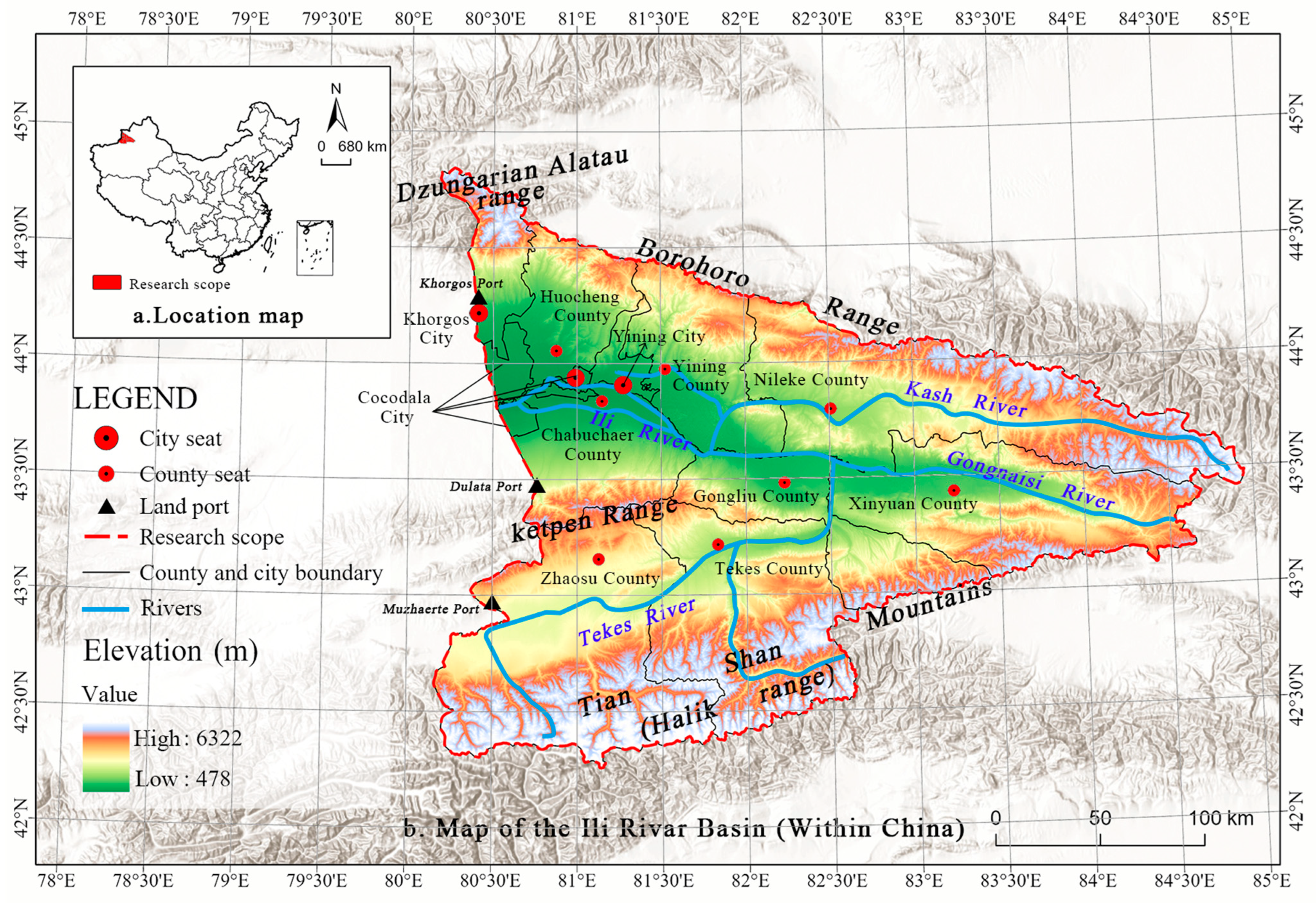
The IRB in China (42°14′16″–44°53′30″ N, 80°09′42″–84°56′50″ E) is located in the interior of Central Asia in the western part of XUAR (Figure 1), with an area of approximately 55,339.16 km2, including 3 cities and 8 counties. By the end of 2020, the total population of the area was 2,619,200 with a population density of 47 people/km2. The study area encompasses the following three border ports: Khorgos, Dulata, and Muzhaerte. The IRB is an area that is a sensitive ecological environment. The “Ili Prefecture Territorial Spatial Planning 2021–2035” positions the IRB as an important hub of the Silk Road Economic Belt, a world-class tourist destination, and a strategic ecological security barrier in Northwest China.
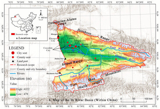
Figure 1.
Geographical map of the study area.
The IBR features complex terrain, with terrain that is higher in the east and lower in the west. It is narrow in the east and wide in the west, resembling a trumpet opening to the west. The Ili River originates from three main feeder streams (the Kash, Gongnaisi, and Tekes Rivers), which descend from the Tian Shan Mountains. The river is surrounded by the Borohoro and Dzungarian Alatau ranges to the north and the Halik and Ketpen ranges to the south. It flows westward for 1,439 km from its point of origin, exiting China’s XUAR and extending into Kazakhstan [41], with a mean annual discharge of about 480 m3/s [14]. The IRB, which has a typical temperate continental climate characterized by a mean annual temperature of 7 °C [42] and a mean annual precipitation ranging from 200 to 1000 mm, is the wettest region in XAUR [43]. It features a relatively humid climate, well-developed vegetation, and pasture, making it a typical livestock farming base in China [44].
2.1.2. Data Sources
This study focuses on the TZS of the IRB, analyzing its distribution, scale, spatial transformation, and driving mechanisms. To ensure data consistency, the administrative units of 2020 were used as the reference. The necessary data are listed in Table 1.

Table 1.
Data sources.
2.2. Methods
2.2.1. Spatial Classification
This article used ArcGIS technology to crop GlobeLand30 data from 2000 to 2020. The overall accuracy of the GlobeLand30 is 83.58% in XUAR, with a kappa coefficient of 0.717 [47]. Based on the GlobeLand30 classification of land use types, the nine distinct categories within the region were subsequently grouped into three overarching spaces as follows: “ecological space, agricultural space, and urban space” (Table 2). Urban space (US) primarily consists of artificial surfaces, while agricultural space (AS) is predominantly cultivated land. The special characteristics of bareland in the basin ecological space (large-scale and concentrated bareland; obvious cross-conversion with forest, shrubland, and other land uses; and dominant functions and ecological services are different from forest and other land uses) necessitated its classification into two subcategories as follows: “green ecological space” (GES) and “other ecological space” (OES).
Table 2.
The classification scheme of “three-zone space” in the Ili River Basin.
Therefore, this paper established the TZS classification system in the IRB by taking land dominant functions as the starting point, combining relevant studies with the actual situation of the basin. This study analyzed the evolutionary characteristics of US, AS, OES, and GES.
2.2.2. “Three-Zone Space” Dynamic Degree
The dynamic degree serves as a measure to quantify both the rate of transformation and the extent of change that various geographical functional areas undergo within a specified time frame in research on land use change [48,49].
where K represents the dynamic degree, or the rate of change, of a particular spatial type over a defined time period. Ua signifies the initial area occupied by this spatial type at the start of the period, whereas Ub denotes its area at the conclusion of the period. T stands for the length of this time period.
2.2.3. Kernel Density Estimation
Kernel density estimation can help us understand the spatial distribution patterns of data points [50]. This study utilized ArcGIS 10.8 software to analyze the spatial distribution characteristics of the transformed area within the TZS. After comparing kernel density analysis maps under various search radii, a 10 km search radius was adopted, as it better depicted the spatial distribution. The formula is as follows:
where Fn(x) serves as an approximation for the kernel density value for the search radius, denoted as h (h > 0). n signifies the total count of samples that represent spatial transitions within the studied area. The k function quantifies the distance between any given point element x and a reference point xi.
2.2.4. Space Pattern Transfer Matrix
A land use transfer matrix can visualize the overall change in land use types [51]. This study employed a land use transfer matrix as a tool for quantitatively describing the transformation of TZS. In Table 3, i = 1, 2, … J represents the space type at the initial time point and j = 1, 2, … J represents the space type at the final time point, where J is the number of space types. T is the number of time points, Yt represents the year at time point t, and t represents the index for the initial time point of interval [Yt, Yt+1], where t ranges from 1 to T − 1. Ctij represents the area converted from space type i at time Yt to space type j at time Yt+1. Ctii represents the area of space type i that remains unchanged. represents the total area of space type i at the initial time point. represents the total area of space type j at the final time point. represents the loss in the area of space type i for time interval [Yt, Yt+1]; represents the gain in the area of land use type j for time interval [Yt, Yt+1].
Table 3.
Space pattern transfer matrix from the initial time to the final time.
2.2.5. Change Budget
Based on the spatial change transfer matrix, we can further calculate the spatial change budget [52]. Equation (3) calculates the total change by summing all the entries within the matrix and then subtracting the diagonal entries, which represent persistence. The total change encompasses both quantity change and allocation change.
Equation (4) gives the quantity change. Categories with a positive net change are selected by the MAXIMUM function, followed by a summation over j to accumulate the positive net changes. Equation (5) computes the allocation change, which represents the percentage of total change minus the percentage of quantity change.
2.2.6. Intensity Analysis
The intensity analysis method, grounded in a transfer matrix, constitutes a mathematical framework that compares a uniform intensity with the intensities of temporal variations observed among distinct categories [33,53]. Although this study utilized only a single time interval from 2000 to 2020, we could still employ the interval level of intensity analysis to calculate the annual change during the interval [Yt, Yt+1], which serves as a foundation for subsequent category level analysis. In Equation (6), St represents the observed annual change intensity during interval [Yt, Yt+1].
This study adopted this method at two levels (category and transition) to analyze the intensity characteristics of changes in the TZS.
Equations (7) and (8) show the intensity analysis of the category level, where Gtj represents the annual average increase intensity and Lti represents the annual average decrease intensity. By comparing the values of Gtj, Lti, and St (from Equation (6)), it can be determined whether the increase or decrease in a space type is active or dormant. If Gtj > St, the increase in category j is judged as active; if Gtj < St, the increase in category j is judged as dormant. The same applies to the judgment of space type decrease.
Equations (9) and (10) show the intensity analysis of the transition level, where Rtin represents the intensity of the transformation from other space types to this specific space type and Wtn represents the uniform transition intensity of other space types converting to this space type. If space types n were to gain with the same intensity from all non-i space types, then Rtin would equal Wtn. If Rtin > Wtn, it is judged that space type i tends to convert to space type n; if Rtin < Wtn, it is judged that space type i avoids converting to space type n.
2.2.7. Optimized Parameter Geodetector
The factor detection and interaction detection of the optimized parameter Geodetector (OPGD) [36] was employed to analyze the impact of various factors on the transformation of the TZS.
In practical spatial analysis, continuous variables should be discretized with optimal parameters before modeling. The efficacy of discretization in classification can be assessed through the statistic Q of a geographic detector, where a higher Q value indicates better partitioning. Thus, we employed the GD package in the R language, utilizing methods such as natural breaks, quantile breaks, and others, with the number of classifications ranging from 3 to 8, and selected the parameter combination yielding the highest Q value as the parameter for geographic detector analysis.
Equation (11) show the explanatory power of factors for the transformation of various types of spaces, with the range of Q-statistic values being [0, 1]. The larger the Q, the stronger the explanatory power of the factor for the specific type of spatial transformation. j = 1, …, M represents the strata (or sub-regions) of the explanatory variable v; and represent the number of units in the j-th sub-region of variable v and the whole area, respectively. and are the variances in the j-th sub-region of variable v and the whole area, respectively.
The impacts of two spatial variables were explained by their interactions, which are illustrated by the five interaction types shown in Table 4 [54,55].
Table 4.
Types of interaction between two covariates.
2.2.8. Description of Variables
Considering local circumstances and the factors’ quantifiabilities and availabilities, we selected 18 indicators from the perspectives of economy, society, geography, location, and climate (Table 5). The selected independent variables were stratified using optimal parameter selection, converting them from numerical variables to categorical variables. Then, using the OPGD, detection was conducted for the 12 spatial types in the IRB from 2000 to 2020.
Table 5.
Description of variables and indicators.
3. Results
3.1. Characteristics of Spatial–Temporal Evolution of Land Use Structure
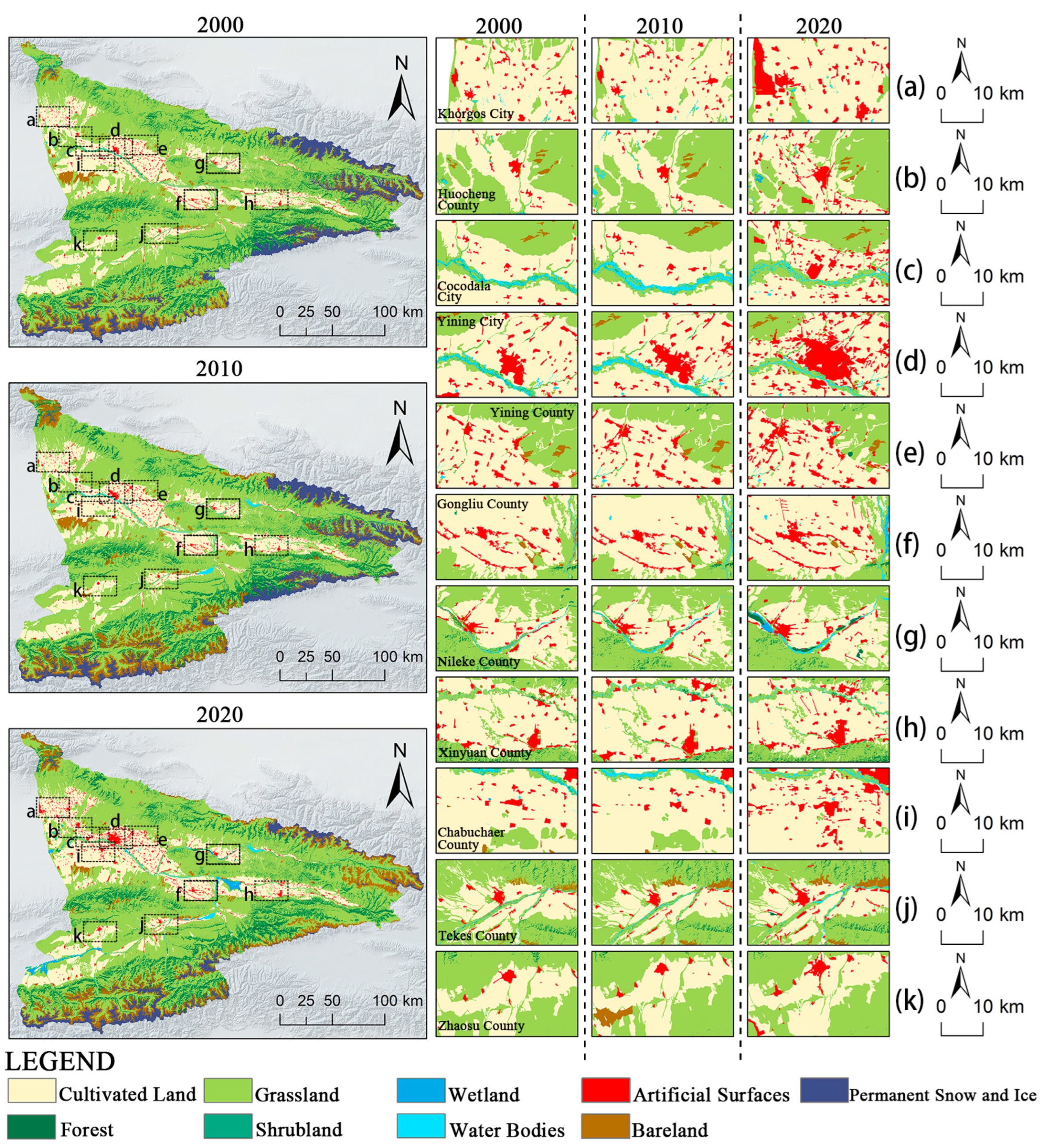
From 2000 to 2020, significant changes were observed in the land use distribution in the IRB (Figure 2 and Table 6). The cultivated land increased by 837.5 km2 over 20 years, with a gradual decline in the first decade and substantial growth in the second. The artificial surfaces expanded by 519.64 km2, with the majority of the increase concentrated in the cities of Khorgos, Cocodala, and Yining, while other counties and cities also experienced different levels of growth.
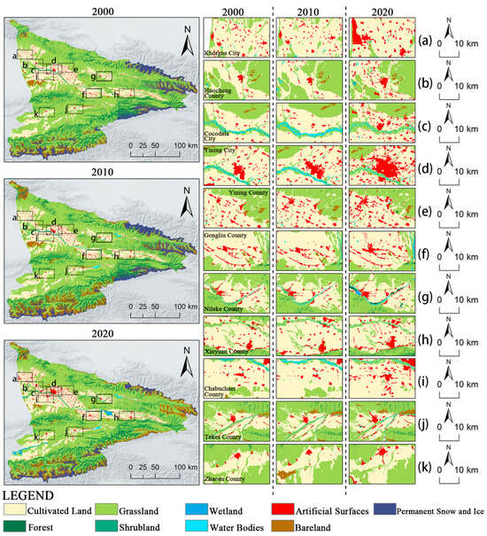
Figure 2.
Land use classification maps of the IRB in 2000, 2010, and 2020. Note: (a) Khorgos City, (b) Huocheng County, (c) Cocodala City, (d) Yining City, (e) Yining County, (f) Gongliu County, (g) Nileke County, (h) Xinyuan County, (i) Chabuchaer County, (j) Tekes County, (k) Zhaosu County.
Table 6.
Land use classification data of the Ili River Basin in 2000, 2010, and 2020.
The reduction of 1469.2 km2 occurred in the grassland, representing a 4.46% decrease. The decline in grassland primarily occurred from 2000 to 2010. During the following decade, the reduction in grassland area was alleviated. Shrubland decreased by 11.64 km2 over a period of 20 years, while bareland increased by 1518.20 km2. Bareland was primarily found in the southern region of the Tian Shan Mountains, the Borohoro range, and Dzungarian Alatau range, intersecting with glacier and permanent snow land as well as forested land. This trend will increase the ecological vulnerability of the IRB. The most substantial growth in land use area was observed in wetlands, with their size increasing from 8.94 km2 in 2000 to 300.60 km2 in 2020, representing a growth rate of 3264.27%. They were primarily located along the riverbanks, and during the same period, the water bodies of the IRB also increased to 381.65 km2, with a growth rate of 112.72%. The expansion of wetland areas was closely linked to the increase in water area. Glaciers and permanent snow land saw the most significant decrease in area, declining by 1996.83 km2, which was attributed to global warming and the overall temperature rise in the IRB [15]. Meanwhile, the melting of glaciers and permanent snowfields accelerated the formation of bareland.
3.2. Spatial–Temporal Evolution Characteristics of the “Three-Zone Space” in the Ili River Basin
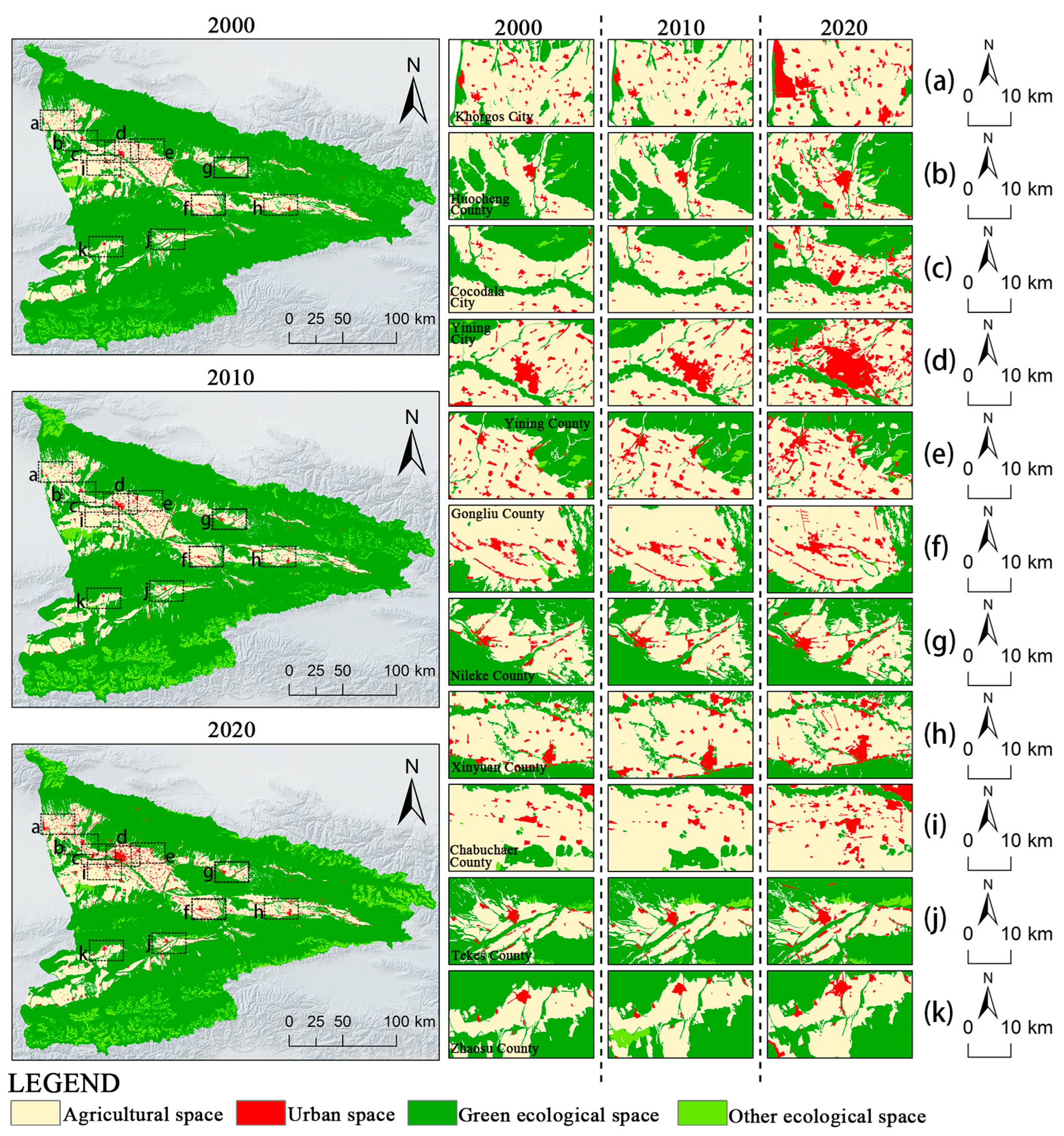
From 2000 to 2020, notable alterations took place in the urban spatial configuration of the IRB (Figure 3 and Table 7). In 2020, US reached 1119.11 km2, accounting for 2.02% of the total study area. Over the course of 20 years, US increased by a total of 519.64 km2, representing a growth rate of 86.68%. This increase was primarily concentrated in newly established cities, such as Khorgos City and Cocodala City, and the surrounding areas of Yining City (Figure 3a–d). The evolution rate of US shifted from stable growth in the first decade to rapid expansion in the second decade (dynamic degree: 0.46 to 7.84%). In terms of spatial distribution, US was primarily distributed along the valley lowlands. Taking Yining City as an example, urbanization led to gradual outward expansion of its US, resulting in the formation of an urban–rural interface with adjacent agricultural areas. From 2000 to 2020, the overall scale of AS underwent a process of initial decline followed by growth (dynamic degree: −0.02 to 0.94%). From 2000 to 2010, there was a slight decrease in AS, amounting to a reduction of 16.31 km2. Over the next decade, there was a stable increase, with a growth scale of 853.81 km2. In 2020, AS reached 9961.07 km2, accounting for 18% of the total study area. Over the course of 20 years, the AS increased by a total of 837.5 km2, representing a growth rate of 9.18%. Notably, the expansion of AS was particularly evident in Chabuchaer County (Figure 3i).
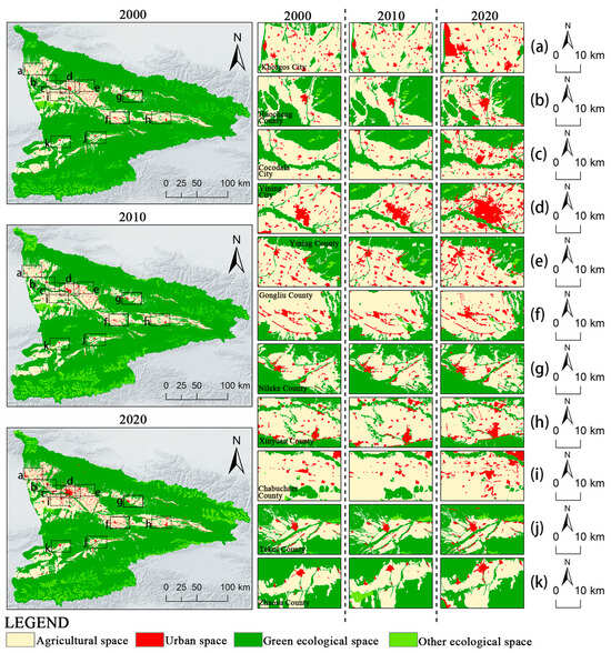
Figure 3.
The three-zone space evolution in the Ili River Basin in 2000, 2010, and 2020. Note: (a) Khorgos City, (b) Huocheng County, (c) Cocodala City, (d) Yining City, (e) Yining County, (f) Gongliu County, (g) Nileke County, (h) Xinyuan County, (i) Chabuchaer County, (j) Tekes County, (k) Zhaosu County.
Table 7.
Spatial changes and dynamic degree of the “Three-zone space” in the Ili River Basin in 2000, 2010, and 2020.
There was a decrease in the scale of ecological space, with the area decreasing from 45,616.13 km2 in 2000 to 44,258.98 km2 in 2020, representing a reduction rate of 2.98%. Furthermore, from a secondary classification standpoint, there was a downward trend in GES. The net decrease in GES from 2000 to 2020 was 2875.97 km2, with a dynamic degree of −0.67%. For OES, the net increase from 2000 to 2010 was 1686.45 km2, with a dynamic degree of 5.75%, and the net decrease from 2010 to 2020 was 167.93 km2, with a dynamic degree of −0.36%. These spaces were mostly situated in the mountainous areas surrounding the IRB.
3.3. Spatial–Temporal Cross-Transformation Characteristics of the “Three-Zone Space”
3.3.1. Change Budget for “Three Zone Space”
According to Table 8, from 2000 to 2020, there was a change in the spatial area of the TZS within the study area. Specifically, US increased by 584 km2, and the increase in OES was the highest, reaching 2799.35 km2. The main reduction was the decrease in GES, with a reduction of 4165.98 km2. The reduction in US was the least, at only 64.36 km2.
Table 8.
Transfer matrix of the three-zone space, 2000–2020 (km2).
Figure 4 shows that the total spatial change in the TZS of the IRB from 2000 to 2020 was 11.07%, comprising both quantity and allocation changes, with quantity change accounting for 5.20% of the total.
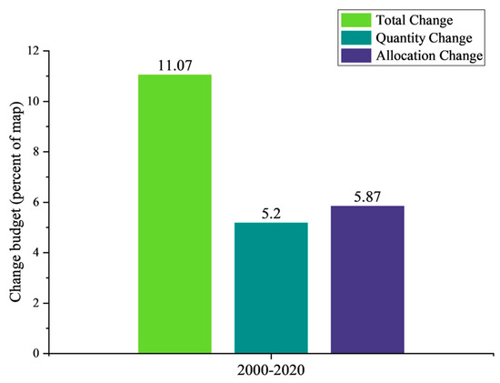
Figure 4.
Total change separated into quantity and allocation.
Figure 5 illustrates the percent gain, persistence, and loss in the total area from 2000 to 2020. By calculating the sum of persistence and gain for each spatial type in the diagram, one can obtain the scale of the corresponding spatial type in 2020. Similarly, by calculating the sum of persistence and loss, one can obtain the scale of the corresponding spatial type in 2000. The percentage of GES had the greatest loss, whereas US had the least. In contrast, the percentage of OES had the largest gain.
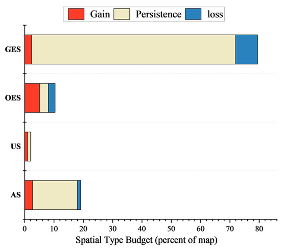
Figure 5.
Gain, persistence, and loss in the TZS, 2000–2020.
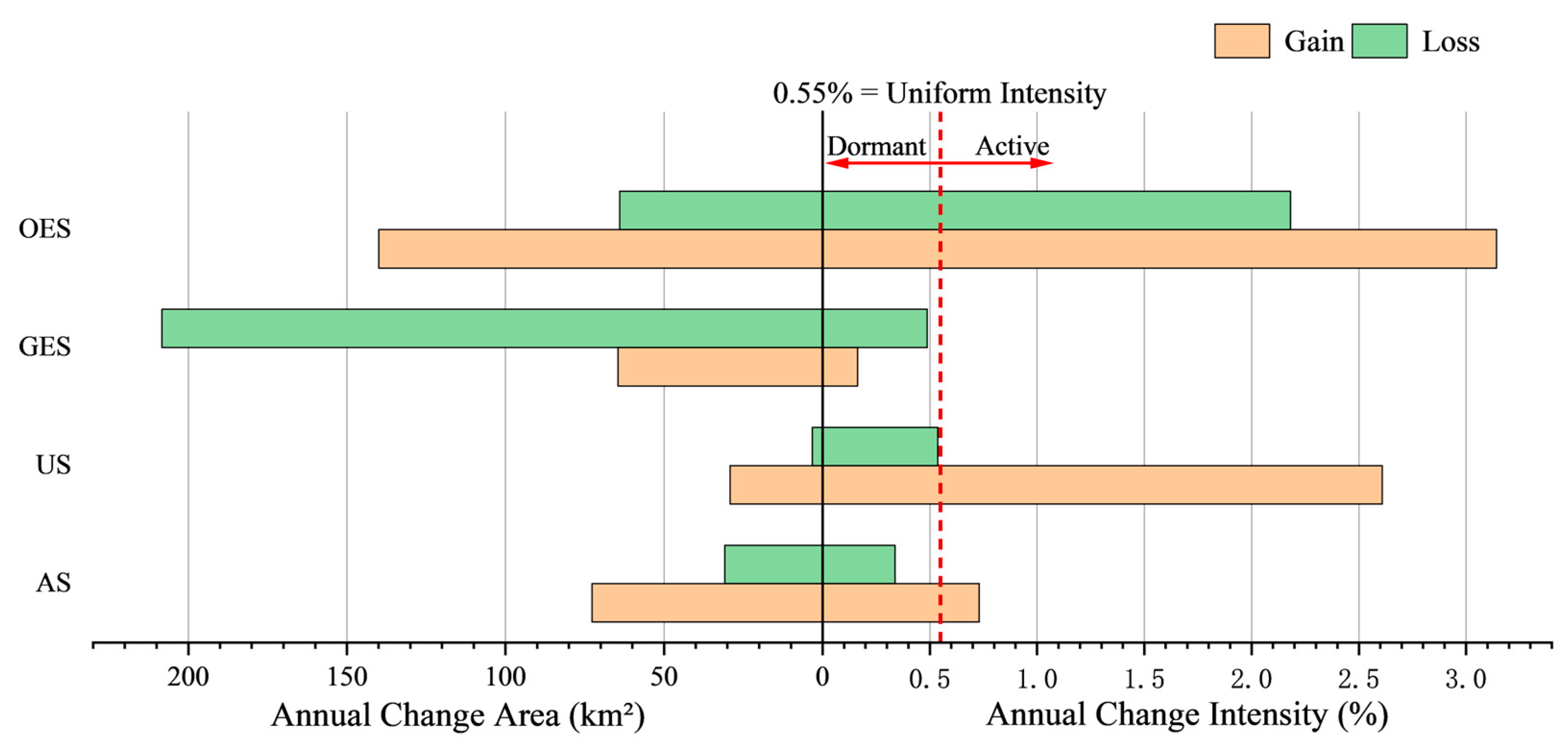
3.3.2. Change Intensity Analysis for the “Three-Zone Space”
Figure 6 shows the intensity of gains and losses by each spatial type from 2000 to 2020. The left side shows that OES had the largest area in terms of annual gains while GES has the largest area in terms of annual losses. The right side of Figure 6 shows the annual transition intensity (St), and the red dotted line represents the uniform intensity line. If the change intensity of a certain spatial type is greater than the uniform line, it indicates that the spatial-type change is active; otherwise, it is dormant. OES was an active loser and active gainer, and OES’s gain was greater than its loss, resulting in a net gain. In contrast, GES was a dormant loser and a dormant gainer, and GES’s loss was greater than its gain, resulting in a net loss. In addition, US and AS were dormant in loss but active in terms of spatial gain.

Figure 6.
Annual change area and intensity of spatial categories’ gains and losses in the IRB during 2000–2020.
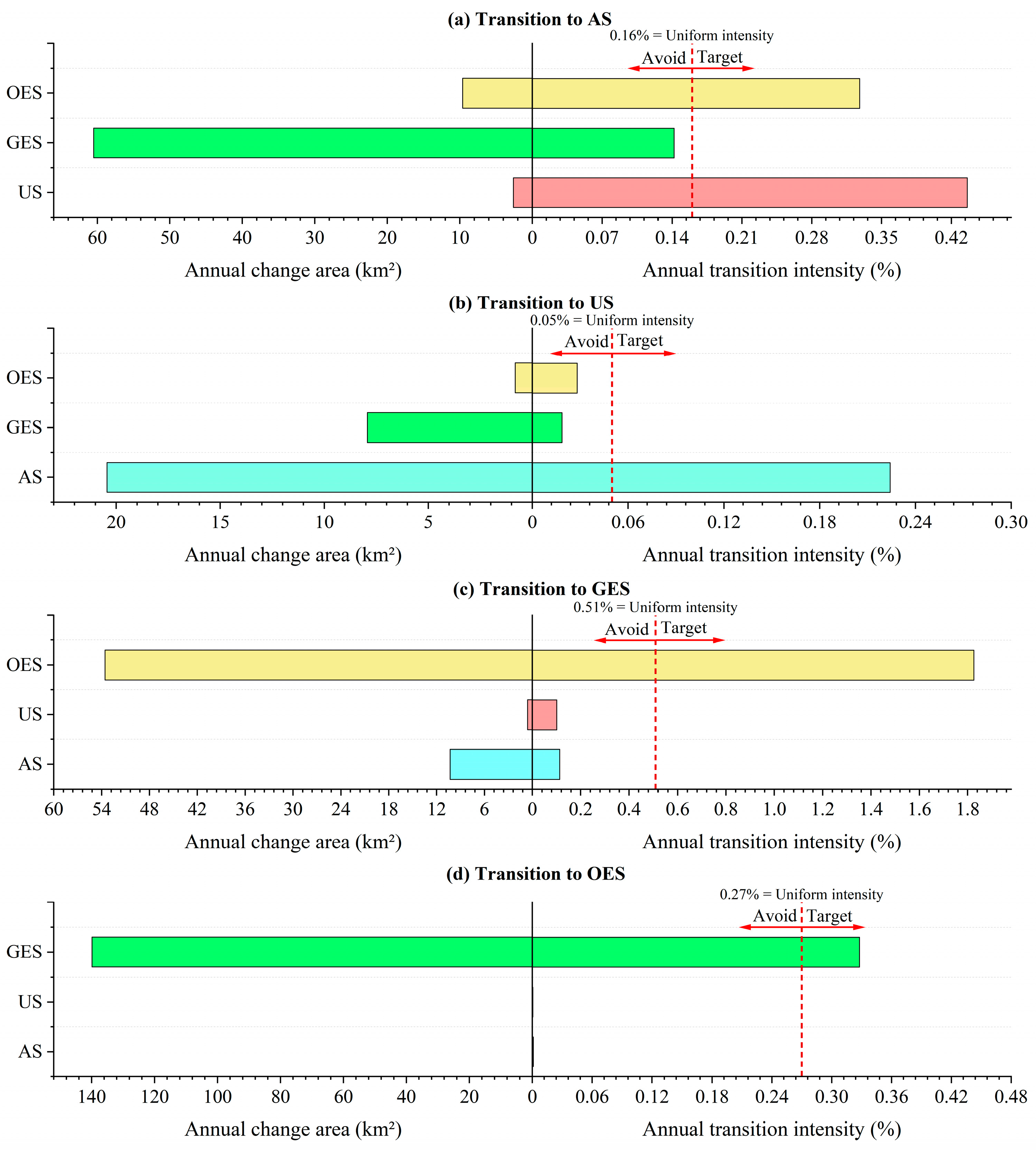
Figure 7 shows the analysis results of transition intensities among the four spatial types from 2000 to 2020, where the red dashed line represents uniform transition intensities. If the transition intensity of a certain spatial type on the right side is greater than the uniform line, then the transition is targeted; conversely, it is avoided.
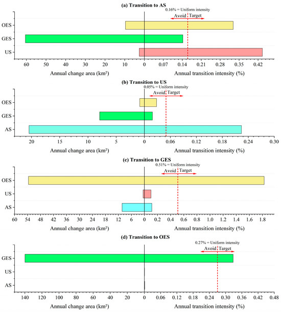
Figure 7.
The gain intensity from losing spatial categories during 2000–2020.
The left side of Figure 7a shows that the largest source of increase for AS was from GES in terms of the annual change area. The right side of Figure 7a shows that the intensity of US transitioning to AS was the highest in terms of the annual transition intensity, followed by the transition of OES to AS, but the transition intensity of GES to AS was the lowest. This indicates that US and OES were more inclined to transition to AS, while GES avoided transitioning to AS. Further explanation is that, although the scale of GES transforming into AS was large, its transition intensity, because of its large initial area, was small and displayed a tendency to avoid.
The left side of Figure 7b shows that the main sources of increase for US were AS and OES in terms of the annual change area. The right side of Figure 7b shows that, in terms of the annual transition intensity, only AS targeted the transition to US specifically. Despite the large area of GES transitioning to US, its transition intensity remained low and displayed a tendency to avoid.
The left sides of Figure 7c,d show that, in terms of the annual change area, the main source of increase for both GES and OES was the other. The right sides of Figure 7c,d show that in terms of the annual transition intensity, GES and OES tended to transition to each other, but the transition intensity of OES to GES was stronger than that of GES to OES.
3.3.3. Spatial Differentiation Characteristics of Cross-Transitions in the “Three-Zone Space”
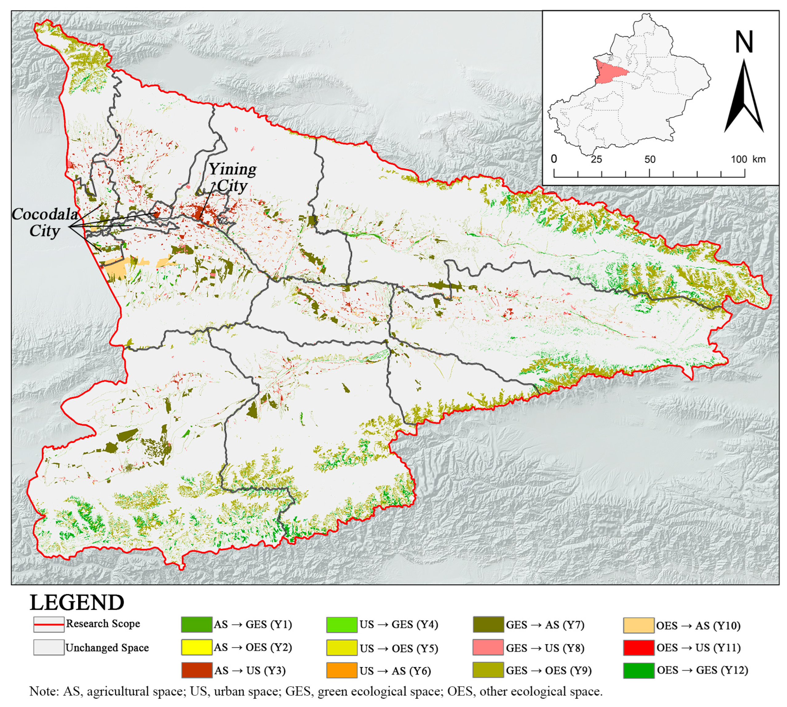
To explore the TZS conversion in the IRB, the TZS transformation matrix for 2000–2020 was obtained (Table 8) and visualized. Figure 8 shows the overall distribution of spatial changes during the period. In order to further study the distribution of various spatial type conversions, the kernel density analysis method was used (Figure 9).
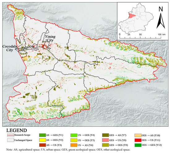
Figure 8.
Cross-conversion map of three-zone space in the Ili River Basin from 2000 to 2020.
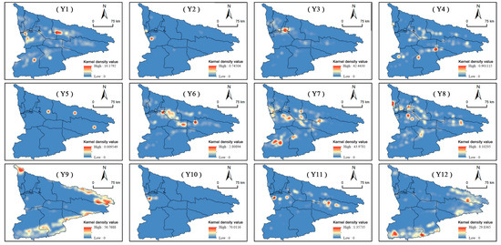
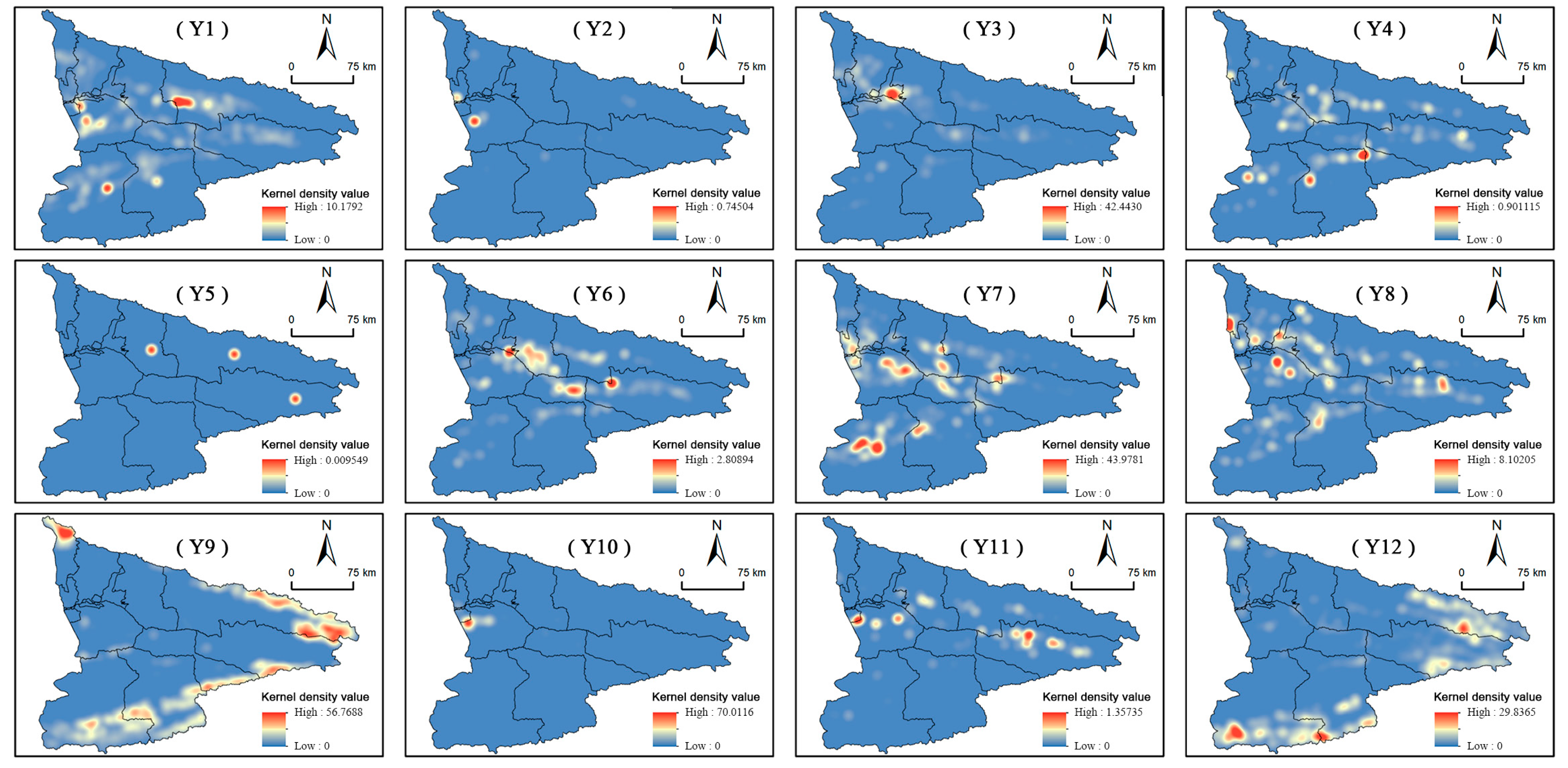
Figure 9.
Spatial characteristics of the kernel density in the IRB for the conversion of the “three-zone space” from 2000 to 2020.
Figure 9 shows that the conversion from AS to GES (Figure 9(Y1)) in 2000–2020 exhibited pronounced spatial clustering characteristics. The high-value areas were mainly distributed in the eastern parts of Nileke County and Chabuchaer County. The spatial clustering of the conversion from AS to OES (Figure 9(Y2)) was high, and the areas with high values were distributed in the western parts of Chabuchaer County. The conversion from AS to US (Figure 9(Y3)) showed obvious spatial clustering characteristics, and the areas with high values were distributed in the southern part of Yining City and Cocadala City.
The high-value areas of the conversion from US to GES (Figure 9(Y4)) were widely distributed, and the spatial agglomeration was low. The high-value areas were mainly distributed in the central part of Nileke County, with secondary occurrences in western Tekes County and Zhaosu County. The spatial clustering of the conversion from US to other AS (Figure 9(Y6)) was high, and the areas with high values were distributed at the confluence of Yining City, Yining County, and Chabuchaer County, as well as the Gongliu County seat and the northwest of Xinyuan County. Notably, the conversion from US to OES (Figure 9(Y5)) from 2000 to 2020 only amounted to 0.05 km2, which was limited to Yining County, Nileke County, and Xinyuan County and lacked a clustered pattern. Because of the sparse sample point data, further analysis of this type of spatial transformation was not conducted.
The GES conversions to AS (Figure 9(Y7)) and to US (Figure 9(Y8)) were mainly distributed in urban suburbs at all levels within the IRB. The spatial clustering of the conversion from GES to OES (Figure 9(Y9)) was high, the areas with high values were distributed in the Dzungarian Alatau range, the eastern regions of Borohoro Mountain, and the southern regions of Tian Shan Mountains in the IRB.
The spatial clustering of the conversion to AS (Figure 9(Y10)) was very high, and the areas with high kernel density values were distributed in the southern area of Cocadala City and the western boundary of Chabuchaer County. Concerning the conversion to US (Figure 9(Y11)), the areas with high values were distributed in the counties and cities along the Ili River and the Gongnaisi River. The spatial clustering of the conversion from OES to GES (Figure 9(Y12)) was also high. The analysis of Y9 and Y12 revealed a mutual conversion pattern between OES and GES, demonstrating significant spatial congruence between these two categories of spatial transformation.
3.4. Driving Mechanism
3.4.1. The Conversion of Agricultural Space
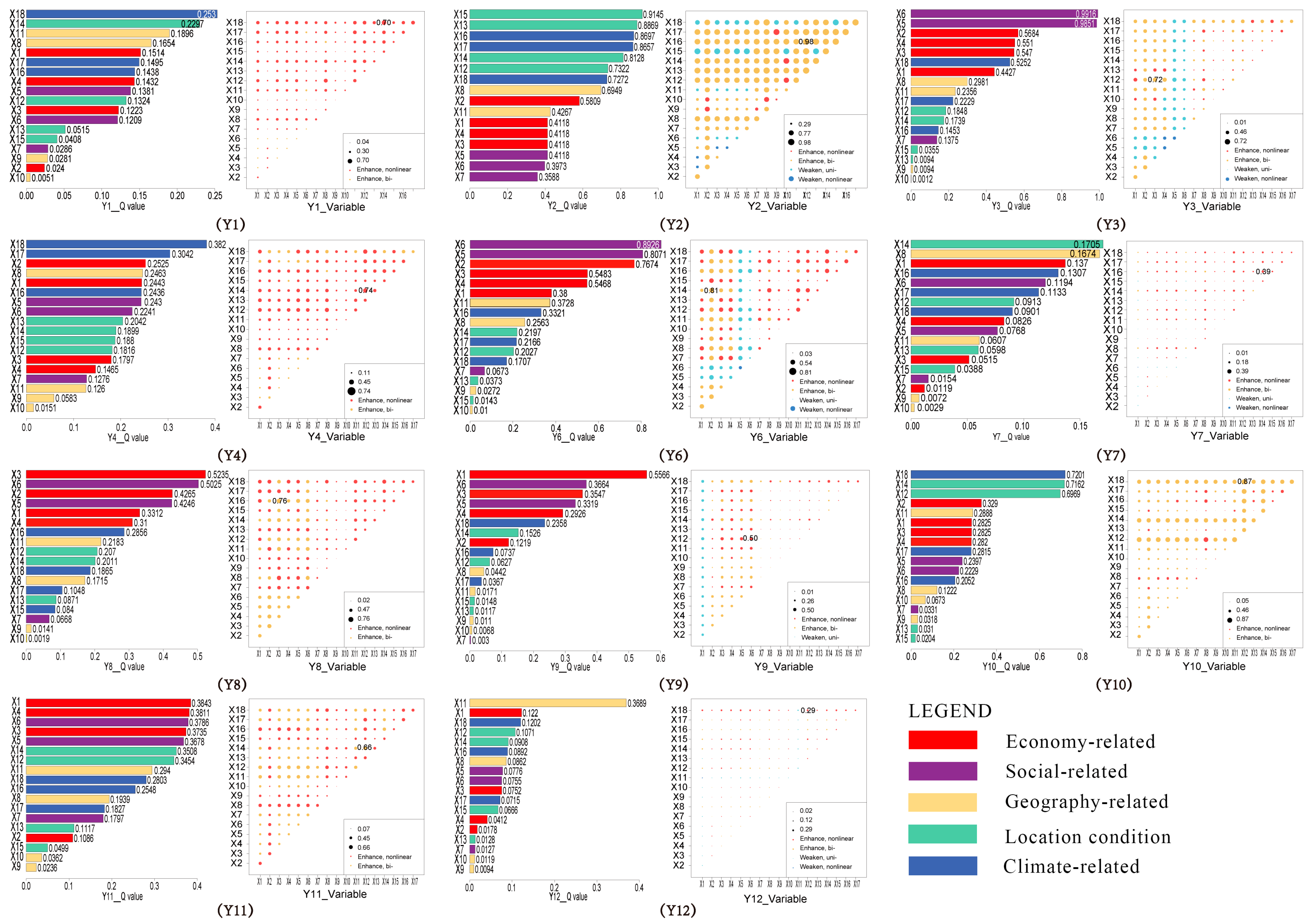
Regarding the conversion from US to AS, the order of the Q-statistic (value > 0.1) was as follows: X6 > X5 > X2 > X3 > X4 > X1 > X11 > X16 > X8 > X14 > X17 > X12 > X18 (Figure 10(Y6)). Therefore, the resident population and urbanization rate were the main factors for the conversion from US to AS. In this conversion process, the interaction among variables demonstrated bi-variable enhancement, nonlinear enhancement, and nonlinear weaken. Regarding the transformation from OES to AS (Figure 10(Y10)), the variables with an influence (Q > 0.2) were X18, X14, X12, X2, X11, X1, X3, X4, X17, X5, X6, and X16. In this transformation process, all variables exhibited bi-variable enhancement or nonlinear enhancement, indicating that the interaction effects among variables enhanced the explanatory power of the conversion from OES to AS to varying degrees. The interaction between X18 and X12 demonstrated bi-variable enhancement, with the highest interaction statistic reaching 0.87. Based on the location advantages of the newly built Cocodala City, it drove agricultural development in surrounding areas, thereby promoting the transformation from OES to AS.

Figure 10.
Geodetector results for the “three-zone space”. Note: 1. In each group, the bar chart on the left shows the results of the factor detector, while the heat map on the right shows the results of the interactive detector. 2. Output value of primary production (X1), nighttime light index (X2), local general budget revenue (X3), local general budget expenditure (X4), resident population (X5), urbanization rate (X6), population density (X7), elevation (X8), slope (X9), slope aspect (X10), soil type (X11), the average distance to city and county seats (X12), average distance to rivers (X13), average distance to railways (X14), average distance to roads (X15), average annual temperature (X16), average annual precipitation (X17), and snow depth (X18). 3. Due to an inadequate number of sampling points in Y5, we are unable to fully leverage geographical detectors for a comprehensive exploration.
Based on a comparison of the q values in all the transformations, the Q-statistic in the conversion from GES to AS (Figure 10(Y7)) was lower than others. The order of the Q-statistic (value > 0.1) was as follows: X14 > X8 > X1 > X16 > X6 > X17. Notably, the interaction between X15 and X16 demonstrated nonlinear enhancement, with an interaction statistic of 0.39. The influence of interactions in locational conditions and climatic factors surpassed the individual effects of each factor. The suitable climatic conditions for agricultural development, along with transportation facilities that facilitate people’s agricultural activities, promoted the transformation of GES into AS.
3.4.2. The Conversion of Urban Space
Regarding the conversion from AS to US (Figure 10(Y3)), the variables with an influence (Q > 0.2) were X6, X5, X2, X4, X3, X18, X1, X8, X11, and X17. The interaction detection results for Y3 revealed that the interaction between X3 and X12 exhibited bi-variable enhancement, with the highest explanatory power reaching 0.7231. The rapid development of towns and cities, which occupied a certain amount of farmland, was the main reason for the transformation of AS into US.
The analysis of driving variables behind the transition from OES to US (Figure 10(Y11)) indicated that these spatial transformations were influenced by variables encompassing economic, social, geographical, locational, and climatic aspects. The order of the Q-statistic (Q > 0.2) was as follows: X1 > X4 > X6 > X3 > X5 > X14 > X12 > X11 > X18 > X16. The interaction detection results for Y11 revealed that all variables exhibited bi-variable enhancement or nonlinear enhancement. X14 and X12 demonstrated bi-variable enhancement, with the highest interaction statistic being 0.66.
In the analysis of the driving factors for the conversion from GES to US (Figure 10(Y8)), the variables with an influence (Q > 0.2) were X3, X6, X2, X5, X1, X4, and X16. This transformation process included bi-variable enhancement or nonlinear enhancement among all variables, indicating that the interaction effects among variables enhanced the explanatory power of these spatial transformations relative to single-variable effects. The interaction between X3 and X16 demonstrated the highest interaction statistic of 0.7645. Social and economic factors constituted the main driving forces. The development of urbanization caused cities to expand outward, inevitably encroaching on GES.
3.4.3. The Conversion of Ecological Space
The order of the Q-statistic (value > 0.1) corresponding to the transition from AS to GES (Figure 10(Y1)) was as follows: X18 > X14 > X11 > X8 > X1 > X17>X16> X4 > X5 > X12 > X13 > X16. The variables with an influence (Q > 0.2) were X18 and X14. The interaction detection results for Y1 revealed a pattern of bi-variable enhancement or nonlinear enhancement among the variables. This suggests that the interaction effects between variables enhanced the explanatory capability of the transition from AS to GES compared with single-factor effects, with differing degrees of strengthening. The largest interaction variables were X18 and X14, and the interaction statistic was 0.701. This indicates that both climatic factors and location conditions significantly impacted the spatial transformation of this type. The areas with certain water resources and relatively inconvenient transportation were more likely to undergo a transformation from AS to GES, which is closely related to the government’s policies of returning farmland to forests and other forestry and grassland projects.
Regarding the transformation from US to GES (Figure 10(Y4)), the variables with an influence (Q > 0.2) were X18, X17, X2, X8, X1, X16, X5, X6, and X13. In this transformation process, the interaction among variables demonstrated bi-variable enhancement and nonlinear enhancement. The largest interaction variables were X14 and X12, and the interaction statistic was 0.74. Increasing public green spaces, constructing ecological parks, and other means enhanced the urban ecological environment, leading to the transformation of US into GES.
The analysis of the driving factors for the conversion from OES to GES (Figure 10(Y12)) showed that the order of the Q-statistic (value > 0.1) was as follows: X11 > X1 > X18 > X12. The variables with an influence (Q > 0.2) were X11, with a q value of 0.3683. Among the interaction detection results, the interaction factors between X18 and X12 demonstrated nonlinear enhancement, with the highest value of interaction factors being 0.2937. This indicates that both snow depth and location conditions impacted the spatial transformation of this type.
The analysis of the driving factors behind the transformation of AS into OES (Figure 10(Y2)) revealed that, apart from slope (X9) and slope aspect (X10), the Q-statistic of other driving factors exceeded 0.2. Among them, the Q values of the X15, X16, X13, X1, X14, X12, X18, and X8 variables were greater than 0.6. The interaction between X16 and X12 yielded the highest explanatory power of 0.9841. Therefore, the distance from cities and towns and the climatic conditions were the main reasons for the abandonment of AS.
Regarding the conversion from GES to OES (Figure 10(Y9)), the variables with an influence (Q > 0.2) were X1, X6, X3, X5, X4 and X18. In this transformation process, except for the nonlinear weaken between X1 and the other variables, the other variables exhibited bi-variable enhancement or nonlinear enhancement, suggesting that the interaction between X1 and the other factors did not enhance its explanatory power relative to a single variable. Within the interaction outcomes, the interaction factors between X6 and X12 displayed nonlinear-enhancement, with the maximum interaction variable value reaching 0.50.
4. Discussion
4.1. Social and Economic Factors Have a Significant Impact on the Evolution of Urban Space
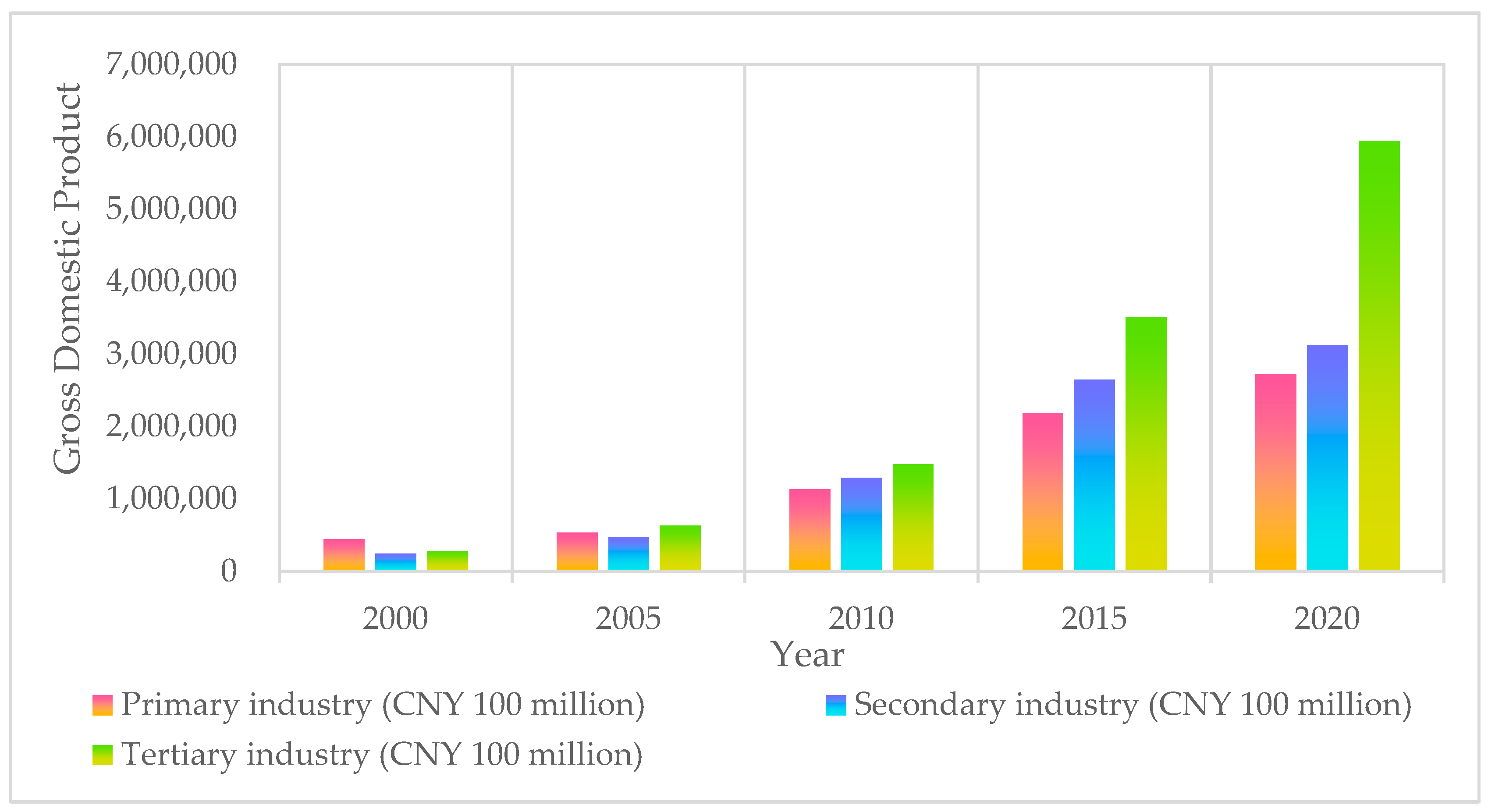
Since 2000, the IRB has experienced rapid development through the pairing assist programs in XUAR [56], economic assistance, the Silk Road Economic Belt [57], and China’s Western Development Strategy [58,59]. In terms of industrial structure changes, the growth rates of the primary, secondary, and tertiary industries have reached 515.59%, 1186.89%, and 2006.50%, respectively (Figure 11). The rapid development of the tertiary industry also resulted in a shift in its proportion from 29.2% in 2000 to 50.4% in 2020, compared with the primary and secondary industries, which changed from 45.7% and 35.4% to 23.1% and 26.5%, respectively. This shift aligns with the increase in US within the IRB. Under the background of urbanization and industrialization, the territorial space pattern of the IRB underwent changes.
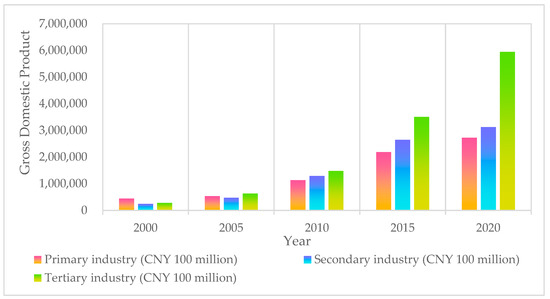
Figure 11.
Trend of industrial changes in the Ili River Basin from 2000 to 2020.
Since 2000, US expanded significantly. US was primarily distributed along the banks of the Ili River, Kash River, Tekes River, and other rivers in the valley lowland, with urban sprawl expanding outward from the city center into surrounding agricultural areas and intersecting with them, causing the patch shape to become complex and the level of space fragmentation to become larger (Figure 3). The conversion of US was primarily sourced from AS (0.74%), followed by GES (0.29%) and OES (0.03%). The factors influencing their conversions were predominantly human factors and exhibited significant spatial heterogeneity. In the case of AS→US (Y3), social and economic factors played the predominant driving roles, with the urbanization rate and resident population as the main driving factors. As for the conversion of GES→US (Y8) and OES→US (Y11), social and economic factors also made the greatest contribution. Compared with ecological space, AS incurred lower construction costs and was more readily converted to US. The expansion of US was concentrated in Khorgos City, Cocodala City, and Yining City. As the capital of the autonomous prefecture, Yining City serves as a regional transportation hub, with a population of 778,000 residents as of 2020, boasting relatively high levels of fiscal revenue, expenditure, and urbanization rates. This signifies that elevated levels of economic development can lead to greater conversion capabilities. Cocodala City, established in 2015 and positioned as a part of the XUAR border urban belt, is located between Khorgos City and Yining City. Its urban development has been bolstered by support from both national and local strategies. Because of urban construction needs, Cocodala City boasts the highest general fiscal revenue and expenditure in the region. The acceleration of urban construction and economic investment has promoted the expansion of US. Khorgos City, home to Khorgos Port, is one of the largest land ports in Central Asia. It has experienced rapid growth in border trade. In 2020, the import and export cargo volume at Khorgos Port reached 34.4162 million tons, ranking first among XUAR ports, with an import and export trade value of CNY 242.65 billion. This enhanced its status as a land port city, attracting large flows of people, goods, and information, thus driving US expansion.
4.2. The Scale of Agricultural Space Did Not Change Significantly
AS increased from 9,123.57 km2 in 2000 to 9,961.07 km2 in 2020. On the one hand, 408.86 km2 of AS was converted to US. On the other hand, 1209.95 km2 of GES, 192.51 km2 of OES, and 52.25 km2 of US were used to supplement AS. Therefore, the overall AS remained stable with consistent growth within the IRB. This is different from the situation in the adjacent area in Almaty province, Kazakhstan, where there was a decrease in cultivated land and an increase in grassland [60]. The Chinese government has implemented a “requisition–compensation balance” policy of cultivated land [61]. The government has resolutely stopped the “non-agricultural” use of cultivated land and implemented a high-standard cultivated land construction action plan to improve the quality and productivity of cultivated land.
The conversion of AS was primarily sourced from GES (2.19%), followed by OES (0.35%) and US (0.09%). The factors influencing their conversions were predominantly natural factors. In the case of GES→AS (Y7) and OES→AS (Y10), locational factors and geographical factors played a predominant driving role. This spatial transformation entails a comprehensive assessment of transportation, arable land suitability, and snow depths in OES, fulfilling the requirements for agricultural development. The presence of convenient transportation and a favorable climate accelerates agricultural development, facilitating the transformation of GES and OES into AS. Regarding the conversion of US, social and economic factors made the highest contribution. The scale of the transition from US to AS (Y6) was relatively small between 2000 and 2020. Social and economic factors such as the permanent population, urbanization rate, and local general budget revenue and expenditure significantly influenced this transition. Polarization and redistribution of the population in the region and rapid urbanization led to the degradation of inefficient land use in some peripheral towns and villages into AS, which optimized the structure of AS.
4.3. Human and Natural Factors Led to the Degradation of Ecological Space
The IRB is situated in the western Tian Shan Mountains and is surrounded by mountains on three sides. It features prevalent westerly winds and abundant precipitation, making it a “wet island” in Central Asia, though it remains part of the arid inland region. Global climate change has impacted the IRB’s ecological environment, making it an ecologically fragile area and an important ecological functional zone in China. Under the influence of the policies of returning farmland to forest (grass), returning grazing land to grasslands, natural forest resources protection, and ecological civilization construction, ecological issues have been emphasized. Our research found that from 2000 to 2020, OES in the IRB, mainly bareland, increased by 1518.82 km2, while GES decreased by 2875.97 km2.
The conversion of GES is primarily sourced from OES (1.94%), followed by AS (0.37%). The transformation from AS to GES (Y1) tended to occur in remote areas with far from towns because of transportation inconveniences. This conversion was mainly concentrated in Nileke County and Chabuchaer County. Nileke County is surrounded by high mountains, has intensified its efforts to protect the ecological environment, including land, forests, and water systems, and is actively creating a practical innovation base for the concept that “lucid waters and lush mountains are invaluable assets.” Through measures such as afforestation of barren mountains and environmental management, it has promoted the improvement and enhancement of the ecological environment. In Chabuchaer County, conversions from AS to GES are closely tied to the government’s ongoing efforts to promote the protection and restoration of natural forests, as well as the implementation of grassland restoration projects, such as the “returning grazing land to grasslands” and “returning farmland to forests and grasslands” policies.
The conversion of OES was primarily sourced from GES (5.05%). In the conversion from GES to OES, economic, social, and climatic factors played major driving roles. On the one hand, the encroachment of other spaces on GES led to the degradation of green spaces. On the other hand, the conversion of GES to OES often occurred in mountainous areas, where various geological activities and climate changes caused glaciers and perennial snow to melt, forming bareland. Regarding the conversions from OES to US (Y11), climatic and locational factors played the predominant role. Such transformations typically occurred in areas abundant in water resources at the periphery of cities, closely intertwined with the implementation of regional ecological conservation projects. This was mainly concentrated in Cocodala City and Xinyuan County, which are expanding their urbanization processes by utilizing OES. In conversions from OES to GES (Y12), geographical and locational factors played dominant roles, which were distributed in high-altitude areas at around 3000 m.
Notably, the mutual transformation between GES and OES was significant and demonstrated a clear spatial congruence in these two categories of spatial transformation (Figure 9(Y9,Y12)). This transformation was primarily distributed in the southern region of the Tian Shan Mountains, the Borohoro range, and the Dzungarian Alatau range, overlapping with the distribution of glaciers and permanent snow cover. The reduction in glacier and permanent snow cover areas led to an increase in OES (Figure 2). Glaciers, as “solid reservoirs,” are crucial sources of replenishment for many rivers in arid regions, playing a vital role in maintaining regional ecological stability and regulating river runoff. The existing research indicates that the snowline elevation in various regions of the Tian Shan Mountains showed a fluctuating upward trend from 2001 to 2015. The average snowline elevation in the Tian Shan Mountains is 3690 m, with a significant upward trend rate of 276 m per decade. Meanwhile, the snowline in the IRB is 3390 m, with a trend rate of 180 m per decade [62]. The meteorological factors most closely related to glacier changes are temperature and precipitation. In recent decades, XUAR has experienced rising temperatures and increased precipitation, which have profoundly impacted glacier reserves. The rise in temperature accelerates glacier melting, which partially offsets the replenishment of glaciers from increased precipitation, promoting glacier melting. Consequently, the increased meltwater is a rising trend in the runoff of glacier-fed rivers in the Tian Shan region of XUAR [63]. This trend also explains the increase in water bodies and wetland areas in the IRB (Figure 2). The conversion of OES to GES in mountainous regions resulted from the natural growth and evolution of bareland vegetation, driven by climate warming and increased rainfall over the 20-year period. Vegetation indices vary with different altitudes. According to the existing research in the IRB, vegetation in areas with elevations below 500 m, between 500 and 1000 m, and above 3000 m has shown an improving trend, while vegetation in areas with elevations between 1000 and 3000 m has experienced vegetation degradation [64]. Consequently, the rise in the snowline and glacier melting leads to the emergence of bareland, which forms new OES through natural restoration processes. This indicates that the IRB should place greater emphasis on managing ecological space and effectively controlling the reduction in ecological space, which will lead to the future development of the social economy in a greener and higher-quality direction.
4.4. Research Significance and Limitations
To understand the inherent mechanisms of spatial evolution and interactions among spaces in the region, an in-depth interactive study from the TZS perspective was conducted. The findings provide a basis for the governance and protection of the IRB, offering guidance for sustainable land management. This paper selected variables from five aspects, including economy, society, geography, location conditions, and climate, to analyze the driving mechanisms of the TZS in the IRB. However, to form a complete theoretical framework of driving mechanisms, further exploration is still required. Because data are difficult to obtain, only district- and county-level indicators were selected. The impact factors also have shortcomings. Subsequent studies can consider indicators such as policy systems, legal regulations, and other indicators, improve the selection of indicators, and fully explore the factors affecting the development of the TZS.
5. Conclusions
The ecological environment of the IRB is of great significance to the ecological security of Northwest China and Central Asia. Based on the territorial spatial governance framework of the TZS, this paper analyzes the long-term spatiotemporal evolution characteristics of the TZS in the IRB and examines the inherent driving mechanisms of its evolution. The following conclusions are drawn from this study.
First, from 2000 to 2020, the AS in the IRB experienced a net increase of 837.51 km2, with a dynamic degree of 0.92%, indicating a gradual expansion trend. US and OES expanded by 519.64 km2 and 1518.83 km2, with the dynamic degrees of 8.67% and 5.17%, respectively, showing significant expansion trends in these two spatial categories. Conversely, GES reduced by 2875.97 km2, with the dynamic degree recorded at −0.67%, signaling a declining trend. Taking 2010 as a pivotal year, the trends manifested as a “decline–rise” in AS, “rise–rise” in US, “rise–decline” in OES, and “decline–decline” in GES.
Second, from intensity analysis, the total TZS change in IRB was 11.07%. At the spatial-type level, both the increase and decrease intensities of OES were active, while those of GES were dormant. The increased intensities of US and AS were active, but their decreased intensities were dormant. The increase in AS mainly came from US and OES, while the increase in US was mainly sourced from AS. The main source of increase for both GES and OES was each other. In terms of spatial transformation intensity, US and OES tended to transform into AS; AS tended to transform into US; and OES and GES had a mutual transformation tendency.
Third, during the 20 years, 12 types of space transformations occurred within the study area. AS converted into US, especially around emerging cities like Khorgas and Cocodala. Additionally, the conversion towards GES was scattered, which encompassed a wider spatial range. The mutual conversion between OES and GES showed spatial distribution consistency, mainly occurring in the Borohoro ranges and the Halik ranges.
Finally, regarding the driving mechanisms, the evolution of US in the IRB was driven by social and economic factors. Location and climate factors accelerated agricultural development, facilitating the transformation of GES and OES into AS. Climate and economic factors played a crucial role in the scale of conversions between OES and GES.
Author Contributions
Conceptualization, M.Y.; methodology, Z.J. and M.Y.; software and visualization, Z.J. and L.Y.; validation, Z.J. and M.Y.; formal analysis, Z.J.; investigation, Z.J., W.S. and L.Y.; resources, Z.J.; data curation, Z.J., W.S. and Z.L.; writing—original draft preparation, Z.J. and M.Y.; writing—review and editing, M.Y.; supervision, Z.J. and M.Y.; project administration, M.Y.; funding acquisition, M.Y. All authors have read and agreed to the published version of the manuscript.
Funding
This research was funded by the National Natural Science Foundation of China (Grant No. 82260414) and the Social Science Fund Project of XPCC (Grant No. 21YB12).
Data Availability Statement
Data are contained within the article.
Acknowledgments
We are sincerely grateful for the editors and reviewers who commented on this paper and gave their time and effort. Finally, we would like to thank the National Natural Science Foundation of China and the Social Science Fund Project of XPCC for their support of this study.
Conflicts of Interest
The authors declare no conflicts of interest.
References
- Transforming Our World: The 2030 Agenda for Sustainable Development. Available online: https://digitallibrary.un.org/record/3923923?v=pdf (accessed on 31 July 2024).
- Allen, C.; Metternicht, G.; Wiedmann, T. Priorities for science to support national implementation of the sustainable development goals: A review of progress and gaps. Sustain. Dev. 2021, 29, 635–652. [Google Scholar] [CrossRef]
- Lovell, S.T. Multifunctional Urban Agriculture for Sustainable Land Use Planning in the United States. Sustainability 2010, 2, 2499–2522. [Google Scholar] [CrossRef]
- Fan, J.; Zhou, K.; Chen, D. Innovation and practice of economic geography for optimizing spatial development pattern in construction of ecological civilization. Econ. Geogr. 2013, 33, 1–8. [Google Scholar] [CrossRef]
- Lambin, E.F.; Meyfroidt, P. Global land use change, economic globalization, and the looming land scarcity. Proc. Natl. Acad. Sci. USA 2011, 108, 3465–3472. [Google Scholar] [CrossRef]
- Wang, W.; Hu, Y.; Zhang, Y. “Ecological-living-industrial” Space Structure Cognition Transformation Control Framework. China Land Sci. 2020, 34, 25–33. [Google Scholar] [CrossRef]
- Wang, G.L.; Yang, D.G.; Xia, F.Q.; Zhong, R.S.; Xiong, C.H. Three types of spatial function zoning in key ecological function areas based on ecological and economic coordinated development: A case study of Tacheng Basin, China. Chin. Geogr. Sci. 2019, 29, 689–699. [Google Scholar] [CrossRef]
- Song, R.; Hu, Y. Comprehensive zoning of land consolidation potential in cities of China and optimization pathways. J. Geo-Inf. Sci. 2020, 22, 1522–1531. [Google Scholar] [CrossRef]
- Yue, W.Z.; Wang, T.Y.; Zhen, Y.L. Unified zoning of territorial space use control derived from the core concept of “Three Types of Spatial Zones and Alert-lines”. China Land Sci. 2020, 34, 52–59. [Google Scholar] [CrossRef]
- Wang, Y.; Liu, X.L.; Wei, X.H.; Yu, H.W. The method and practice of regional spatial planning from “three basic spaces” to “three-zones and three-lines”. Urban Plan. Forum 2018, 4, 65–74. [Google Scholar] [CrossRef]
- Xu, X.L.; Na, R.; Shen, Z.C.; Deng, X.J. Impact of Major Function-Oriented Zone Planning on Spatial and Temporal Evolution of “Three Zone Space” in China. Sustainability 2023, 15, 8312. [Google Scholar] [CrossRef]
- Fan, J. Spatial organization pathway for territorial function-structure: Discussion on implementation of major function zoning strategy in territorial spatial planning. Geogr. Res. 2019, 38, 2373–2387. [Google Scholar] [CrossRef]
- Petr, T. Lake Balkhash, Kazakhstan. Int. J. Salt Lake Res. 1992, 1, 21–46. [Google Scholar] [CrossRef]
- Panyushkina, I.P.; Meko, D.M.; Macklin, M.G.; Toonen, W.H.J.; Mukhamadiev, N.S.; Konovalov, V.G.; Ashikbaev, N.Z.; Sagitov, A.O. Runoff variations in Lake Balkhash Basin, Central Asia, 1779–2015, inferred from tree rings. Clim. Dyn. 2018, 51, 3161–3177. [Google Scholar] [CrossRef]
- Sun, H.L.; Chen, Y.N.; Li, W.H.; Li, F.; Chen, Y.P.; Hao, X.M.; Yang, Y.H. Variation and abrupt change of climate in Ili River Basin, Xinjiang. J. Geogr. Sci. 2010, 20, 652–666. [Google Scholar] [CrossRef]
- Tekir, G. Economic and Political Impacts of the Belt and Road Initiative on Kazakhstan. Int. J. Arts Humanit. Soc. Stud. 2022, 4, 60–69. [Google Scholar]
- Wang, Z.S.; Li, W.F.; Li, Y.S.; Qin, C.B.; Lv, C.Y.; Liu, Y. The “Three Lines One Permit” policy: An integrated environmental regulation in China. Resour. Conserv. Recycl. 2020, 163, 105101. [Google Scholar] [CrossRef]
- Wang, H.Z.; Guo, X.Y.; Liu, T.; Xu, H. Framework and function of “Three Lines and One Permit”: A preemptive and integrated policy for the environmental impact assessment system in China. Environ. Impact Asses. 2022, 94, 106763. [Google Scholar] [CrossRef]
- Lu, Z.; Deng, X. Regional Policy And Regional Development: A Case Study Of China‘s Western Development Strategy. Ann. Univ. Apulensis Ser. Oeconomica 2013, 1, 250–264. [Google Scholar] [CrossRef]
- Feng, C.; Zhang, H.; Xiao, L.; Guo, Y. Land Use Change and Its Driving Factors in the Rural-Urban Fringe of Beijing: A Production-Living-Ecological Perspective. Land 2022, 11, 314. [Google Scholar] [CrossRef]
- Wang, Y.B.; Zhao, R.T.; Li, Y.; Yao, R.; Wu, R.X.; Li, W.L. Research on the evolution and the driving forces of land use classification for production, living, and ecological space in China’s Qilian Mountains Nature Reserve from 2000 to 2020. Environ. Sci. Pollut. Res. 2023, 30, 64949–64970. [Google Scholar] [CrossRef]
- Li, Y.; Song, Y.G.; Fitzsimmons, K.E.; Chen, X.L.; Wang, Q.S.; Sun, H.Y.; Zhang, Z.P. New evidence for the provenance and formation of loess deposits in the Ili River Basin, Arid Central Asia. Aeolian Res. 2018, 35, 1–8. [Google Scholar] [CrossRef]
- Chen, L.; Chen, K.; He, G.; Liu, Z. Research on the Prediction Model of Loess Collapsibility in Xinyuan County, Ili River Valley Area. Water 2023, 15, 3786. [Google Scholar] [CrossRef]
- Zeng, M.X.; Song, Y.G.; Yang, H.; Li, Y.; Cheng, L.Q.; Li, F.Q.; Zhu, L.D.; Wu, Z.R.; Wang, N.J. Quantifying proportions of different material sources to loess based on a grid search and Monte Carlo model: A case study of the Ili Valley, Central Asia. Palaeogeogr. Palaeocl. 2021, 565, 110210. [Google Scholar] [CrossRef]
- Yi, S.; Wang, H.; Yang, S.; Xie, L.; Gao, Y.; Ma, C. Spatial and Temporal Characteristics of Hand-Foot-and-Mouth Disease and Its Response to Climate Factors in the Ili River Valley Region of China. Int. J. Environ. Res. Public Health 2021, 18, 1954. [Google Scholar] [CrossRef]
- He, L. Analysis and Countermeasures on the Present Situation of Water Resources Development and Utilization in Yili River Basin. Shaanxi Water Resour. 2019, 7, 49–51. [Google Scholar] [CrossRef]
- Wang, H.W.; Zhang, X.L.; Qiao, M.; Miao, Y.J. Assessment and dynamic analysis of the eco-environmental quality in the Ili River Basin based on GIS. J. Arid. Land Geogr. 2008, 2, 215–221. [Google Scholar] [CrossRef]
- Wang, Q.; Yang, T.B.; Yang, X.M. The spatio-temporal changes of normalized difference vegetation index and its response to seasonal climate in lli River basin. J. Lanzhou Univ. Nat. Sci. 2016, 52, 466–474. [Google Scholar] [CrossRef]
- Yang, Q.; Yao, J.Q.; Zhao, Y.; Zhao, L.; Han, X.Y.; Zhao, L.; Huang, Y.Z. Spatial-temporal variation of water vapor and its relationship with the precipitation in the Ili River Basin. J. Desert Res. 2012, 33, 1174–1183. [Google Scholar] [CrossRef]
- Wang, C.; Wang, H.W.; Wu, J.H.; He, X.; Luo, K.; Yi, S.Y. Identifying and warning against spatial conflicts of land use from an ecological environment perspective: A case study of the Ili River Valley, China. J. Environ. Manag. 2024, 351, 119757. [Google Scholar] [CrossRef]
- Qi, J.G.; Tao, S.Q.; Pueppke, S.G.; Espolov, T.E.; Beksultanov, M.; Chen, X.; Cai, X.M. Changes in land use/land cover and net primary productivity in the transboundary Ili-Balkhash basin of Central Asia, 1995–2015. Environ. Res Commun. 2020, 2, 011006. [Google Scholar] [CrossRef]
- Pontius, R.G.; Shusas, E.; McEachern, M. Detecting important categorical land changes while accounting for persistence. Agric. Ecosyst. Environ. 2004, 101, 251–268. [Google Scholar] [CrossRef]
- Safaa Zakaria, A.; Robert Gilmore, P. Intensity analysis to unify measurements of size and stationarity of land changes by interval, category, and transition. Landsc. Urban Plan. 2012, 106, 103–114. [Google Scholar] [CrossRef]
- Deng, Z.; Quan, B. Intensity Analysis to Communicate Detailed Detection of Land Use and Land Cover Change in Chang-Zhu-Tan Metropolitan Region, China. Forests 2023, 14, 939. [Google Scholar] [CrossRef]
- Feng, Y.; Lei, Z.; Tong, X.; Gao, C.; Chen, S.; Wang, J.; Wang, S. Spatially-explicit modeling and intensity analysis of China’s land use change 2000–2050. J. Environ. Manag. 2020, 263, 110407. [Google Scholar] [CrossRef] [PubMed]
- Song, Y.Z.; Wang, J.F.; Ge, Y.; Xu, C.D. An optimal parameters-based geographical detector model enhances geographic characteristics of explanatory variables for spatial heterogeneity analysis: Cases with different types of spatial data. Gisci. Remote Sens. 2020, 57, 593–610. [Google Scholar] [CrossRef]
- Du, J.; Zhao, B.; Feng, Y. Spatial distribution and influencing factors of rural tourism: A case study of Henan Province. Heliyon 2024, 10, e29039. [Google Scholar] [CrossRef]
- Xia, J.N.; Hong, M.Y.; Wei, W. Changes and Driving Forces of Urban–Agricultural–Ecological Space in the Yangtze River Economic Belt from 2000 to 2020. Land 2023, 12, 1014. [Google Scholar] [CrossRef]
- Tian, C.J.; Pang, L.H.; Yuan, Q.Z.; Deng, W.; Ren, P. Spatiotemporal Dynamics of Ecosystem Services and Their Trade-Offs and Synergies in Response to Natural and Social Factors: Evidence from Yibin, Upper Yangtze River. Land 2024, 13, 1009. [Google Scholar] [CrossRef]
- Kheyruri, Y.; Sharafati, A.; Neshat, A.; Hameed, A.S.; Rahman, A. Analyzing the impact of socio-environmental parameters on wheat and barley cultivation areas using the geographical detector model. Phys. Chem. Earth Parts A/B/C 2024, 135, 103630. [Google Scholar] [CrossRef]
- Pueppke, S.G.; Zhang, Q.; Nurtazin, S.T. Irrigation in the Ili River Basin of Central Asia: From Ditches to Dams and Diversion. Water 2018, 10, 1650. [Google Scholar] [CrossRef]
- Shi, M.; Wu, H.; Fan, X.; Jia, H.; Dong, T.; He, P.; Baqa, M.F.; Jiang, P. Trade-Offs and Synergies of Multiple Ecosystem Services for Different Land Use Scenarios in the Yili River Valley, China. Sustainability 2021, 13, 1577. [Google Scholar] [CrossRef]
- Jiao, W.; Chen, Y.N.; Li, W.H.; Zhu, C.G.; Li, Z. Estimation of net primary productivity and its driving factors in the Ili River Valley, China. J. Arid. Land 2018, 10, 781–793. [Google Scholar] [CrossRef]
- Yan, J.J.; Liu, H.J.; Cui, D.; Chen, C. Spatiotemporal dynamics of grassland degradation in Yili Valley of Xinjiang over the last 15 years. Pratacultural Sci. 2018, 35, 508–520. [Google Scholar] [CrossRef]
- Xu, H. Land Cover Data (30 m) Derived from Globeland30 for the China Region. Zenodo 2023, 514, 434. [Google Scholar] [CrossRef]
- Xu, X.L. Annual dataset of nighttime lighting in China. Resour. Environ. Sci. Data Regist. Publ. Syst. 2022. [Google Scholar] [CrossRef]
- Liu, J.; Ren, Y.; Chen, X. Regional Accuracy Assessment of 30-Meter GLC_FCS30, GlobeLand30, and CLCD Products: A Case Study in Xinjiang Area. Remote Sens. 2024, 16, 82. [Google Scholar] [CrossRef]
- Ning, J.; Liu, J.Y.; Xu, X.L.; Zhang, S.W.; Yan, C.Z.; Li, R.D.; Wu, S.X.; Hu, Y.F.; Du, G.M.; Chi, W.F.; et al. Spatial-temporal patterns and characteristics of land-use change in China during 2010–2015. J. Geogr. Sci. 2018, 73, 789–802. [Google Scholar] [CrossRef]
- Wang, X.L.; Bao, Y.H. Exploration of land use dynamic change research methods. Prog. Geogr. 1999, 18, 81–87. [Google Scholar] [CrossRef]
- Mazy, F.-R.; Longaretti, P.-Y. Towards a generic theoretical framework for pattern-based LUCC modeling: An accurate and powerful calibration–estimation method based on kernel density estimation. Environ. Model. Softw. 2022, 158, 105551. [Google Scholar] [CrossRef]
- Wei, X.D.; Yang, J.; Luo, P.P.; Lin, L.G.; Lin, K.L.; Guan, J.M. Assessment of the variation and influencing factors of vegetation NPP and carbon sink capacity under different natural conditions. Ecol. Indic. 2022, 138, 108834. [Google Scholar] [CrossRef]
- Pontius, R.G.; Gao, Y.; Giner, N.M.; Kohyama, T.; Osaki, M.; Hirose, K. Design and Interpretation of Intensity Analysis Illustrated by Land Change in Central Kalimantan, Indonesia. Land 2013, 2, 351–369. [Google Scholar] [CrossRef]
- Bin Quan, R.G.P., Jr.; Hui, S. Intensity Analysis to communicate land change during three time intervals in two regions of Quanzhou City, China. GISci. Remote Sens. 2020, 57, 21–36. [Google Scholar] [CrossRef]
- Wang, J.F.; Li, X.H.; Christakos, G.; Liao, Y.L.; Zhang, T.; Gu, X.; Zheng, X.Y. Geographical detectors-based health risk assessment and its application in the neural tube defects study of the Heshun Region, China. Int. J. Geogr. Inf. Sci. 2010, 24, 107–127. [Google Scholar] [CrossRef]
- Wang, J.F.; Zhang, T.L.; Fu, B.J. A measure of spatial stratified heterogeneity. Ecol. Indic. 2016, 67, 250–256. [Google Scholar] [CrossRef]
- Song, T.; Liu, W.; Liu, Z.; Wuzhati, Y. Policy Mobilities and the China Model: Pairing Aid Policy in Xinjiang. Sustainability 2019, 11, 3496. [Google Scholar] [CrossRef]
- Zhang, F.; Wang, Y.; Jim, C.Y.; Chan, N.W.; Tan, M.L.; Kung, H.T.; Shi, J.; Li, X.; He, X. Analysis of Urban Expansion and Human–Land Coordination of Oasis Town Groups in the Core Area of Silk Road Economic Belt, China. Land 2023, 12, 224. [Google Scholar] [CrossRef]
- Lu, Z.; Deng, X. China’s Western Development Strategy: Policies, Effects and Prospects. MPRA Paper No. 35201. 2011. Available online: https://mpra.ub.uni-muenchen.de/35201/1/MPRA_paper_35201.pdf (accessed on 14 October 2023).
- Yang, K.Z. China’s Western Development Strategy for Modernization Drive. J. China Econ. 2021, 16, 62–83. [Google Scholar] [CrossRef]
- Yuan, J.; Chen, J.; Sciusco, P.; Kolluru, V.; Saraf, S.; John, R.; Ochirbat, B. Land Use Hotspots of the Two Largest Landlocked Countries: Kazakhstan and Mongolia. Remote Sens. 2022, 14, 1805. [Google Scholar] [CrossRef]
- Liu, L.; Liu, Z.J.; Gong, J.Z.; Wang, L.; Hu, Y.M. Quantifying the amount, heterogeneity, and pattern of farmland: Implications for China’s requisition-compensation balance of farmland policy. Land Use Policy 2019, 81, 256–266. [Google Scholar] [CrossRef]
- Li, S.A.; Hou, X.G.; Zheng, Z.J.; Zhang, L.C.; Muzhapaer, M.; Xu, Z.D. Monitoring and analysis of snowline on Tianshan Mountains based on remotely sensed data from 2001 to 2015. J. Adv. Water Sci. 2017, 28, 364–372. [Google Scholar] [CrossRef]
- Lan, Y.C.; Shen, Y.P.; Wu, S.F.; Zhong, Y.J.; Wen, J.; Ma, X.B.; Hu, Z.Y. Changes of the glaciers and the glacier water resources in the typical river basins on the north and south slopes of the Tianshan Mountains since 1960s. J. Arid Land Resour. Environ. Impact Assess. Rev. 2007, 21, 1–8. [Google Scholar]
- Li, Y.Q.; Yang, J.H.; Xia, H.B.; Wu, J.J. Spatiotemporal variations of vegetation in the Ili River Basin from 2000 to 2022. J. Arid. Land Geogr. 2024, 47, 741–752. [Google Scholar]


Disclaimer/Publisher’s Note: The statements, opinions and data contained in all publications are solely those of the individual author(s) and contributor(s) and not of MDPI and/or the editor(s). MDPI and/or the editor(s) disclaim responsibility for any injury to people or property resulting from any ideas, methods, instructions or products referred to in the content. |
© 2024 by the authors. Licensee MDPI, Basel, Switzerland. This article is an open access article distributed under the terms and conditions of the Creative Commons Attribution (CC BY) license (https://creativecommons.org/licenses/by/4.0/).