Data-Driven Decision Support to Guide Sustainable Grazing Management

Abstract

Data-driven decision support can help guide sustainable grazing management by providing an accurate estimate of grazing capacity, in coproduction with managers. Here, we described the development of a decision support model to estimate grazing capacity and illustrated its application on two sites in the western United States. For the Montgomery Pass Wild Horse Territory in California and Nevada, the upper limit estimated in the capacity assessment was 398 horses and the current population was 654 horses. For the Eagle Creek watershed of the Apache–Sitgreaves National Forest of eastern Arizona, the lower end of capacity was estimated at 1560 cattle annually, compared to the current average of 1090 cattle annually. In addition to being spatio-temporally comprehensive, the model provides a repeatable, cost-effective, and transparent process for establishing and adjusting capacity estimates and associated grazing plans that are supported by scientific information, in order to support livestock numbers at levels that are sustainable over time, including levels that are below average forage production during drought conditions. This modeling process acts as a decision support tool because it enables different assumptions to be used and explored to accommodate multiple viewpoints during the planning process.

1. Introduction

Rangeland managers are tasked with sustainably achieving multiple-use objectives on public land, including grazing management. Grazing capacity is defined as “the maximum stocking rate that will achieve a target level of animal performance, in a specified grazing method, based on total nutrient resources available, including harvested roughages and concentrates, that can be applied over a defined period without deterioration of the ecosystem” [1]. Stocking rate represents the number of animals on a given amount of land over a certain period [1]. Grazing capacity is related to stocking rate, which is defined as “the relationship between the number of animals and the grazing management unit utilized over a specified time period” [1]. Capacity is most often expressed as animal units and animal unit months. An animal unit (AU) is “Considered to be one mature cow of about 1000 pounds (450 kg), either dry or with calf up to 6 months of age, or their equivalent, consuming about 26 pounds (12 kg) of forage per day on an oven-dry basis” [2]. The animal unit month (AUM) is tantamount to the amount of forage required to sustain an animal unit for 30 days, nominally accepted as 354 kg of oven dried forage [2]. The concept of grazing capacity encompasses consideration for additional social, biological, and ecological elements. For example, managers may need to balance the forage needs of wild ungulates with the needs of permitted livestock [3], or ensure sufficient grass height remains to support greater sage-grouse (Centrocercus urophasianus) [4,5,6] or apply grazing to reduce fuels and fire risk near buildings or households [7]. Grazing capacity is therefore highly dependent on numerous factors that vary seasonally, annually, or over decades, and rarely do managers have detailed, long-term datasets to quantify these factors [8].

Estimates of grazing capacity conventionally have been approximations that are tempered with other information, experience, and judgment [2]. Grazing capacity estimates consider the kind (e.g., grasses, forbs, or shrubs) and amount (i.e., productivity) of vegetation providing forage, as well as the topography, water resources, and multiple-use goals that may affect the availability of that forage. The “stock and monitor” approach involves establishing an initial stocking rate based on estimated grazing capacity, and then analyzing the effects of these stocking levels by measuring forage utilization, spatial and temporal utilization patterns, vegetative composition, riparian health, and soil cover over time [9]. Starting with an accurate estimate of grazing capacity and some sense of its variability over time is critical to being able to quickly adjust livestock numbers to levels that are sustainable over time, yet such information is rarely available. On public lands, the “stock and monitor” approach is recommended for establishing proper livestock stocking rates on grazing allotments since it is, essentially, the adaptive management of the resource, where forage conditions and subsequent use and rangeland health indicators are continually reviewed, and grazing parameters are revised as necessary to meet changes in weather or other environmental factors, as well as changes in management objectives. While the “stock and monitor” approach is simple and often reliable, problems can arise when data are lacking to support revising management decisions. Forage production studies offer a more theoretical approach [10], encompassing landscape features such as slope and distance to water to estimate the amount of usable forage available to a particular kind and class of livestock. Conventional recommendations call for reduced stocking rates on areas with >10% slope and >1.6 km from water because these areas are considered to be less grazed [10,11,12], but these guidelines have been challenged due to an enhanced understanding of cattle terrain use as informed by Global Positioning System (GPS) data [13,14].

Both of these approaches are subject to problems due to a lack of vegetation data, particularly to support revising management decisions when drought limits forage production. Insufficient funding and personnel, along with remote terrain, often prevent the collection of consistent utilization, vegetation, and soil cover data necessary to systematically assess condition and justify changes in stocking, leading to such decisions being based on, at best, limited data. Moreover, the incomplete coverage of variations across space and interannual variability in forage production may not be captured with a few years of measurements.

Furthermore, increased climate variability resulting in more frequent drought now and in the future [15] generates wide variations in forage production from year to year, particularly in semi-arid environments. This can lead to inaccurate assessments of grazing capacity if they are based upon data collected in average (non-drought) years, or are collected from locations that may not fully capture the variation across the landscape. In addition, managers lack a decision support system that can assist in future planning efforts by exploring “what if” scenarios, which are critical for adaptively managing grazing, especially when considering climatic change impacts on rangelands. Taken together, all of these limitations highlight the need for more spatially explicit data describing forage conditions, evaluated in a decision support system that can accommodate differing input assumptions. In light of these issues, the aim of our study was to develop a decision support tool with characteristics of the approach adopted by the authors of [10] but with an improved interaction between the slope and water constraints and provisions for understory forage calculations. In addition, we demonstrate how newly available remotely sensed data sources describing vegetation cover and production can be incorporated into this spatially explicit approach. While the main goal of this work was to develop the decision support system, in this publication we describe case studies of application in support of public land management.

Public lands require estimates of grazing capacity to balance use of the landscape by both wild and domestic ungulates. One such example is found on the Montgomery Pass Wild Horse Territory, which covers approximately 76,000 ha on the California–Nevada border in the western U.S., and jointly managed by the Inyo and Humboldt–Toiyabe National Forests, US Department of Agriculture, Forest Service (USFS) and the US Department of Interior Bureau of Land Management (BLM; Figure 1, Methods). Forest Service regulations direct the Forest Service to “Analyze each wild horse or burro territory and, based on the analysis, develop and implement a management plan, which analysis and plans will be updated, whenever needed, as determined by conditions on each territory” (U.S. Code of Federal Regulations, 36 Part 222 Subpart D). Recent changes in rangeland conditions and wild horse activity have prompted an update to the Territory Management Plan (TML) to ensure that the Montgomery Pass (MP) wild horse herd is being managed in balance with other objectives. This balance is achieved through the establishment and maintenance of Appropriate Management Levels (AMLs), as dictated by BLM and USFS policy. Appropriate Management Level decisions determine the number of wild horses to be managed within an established territory. The AMLs are expressed as a population range with an upper and lower limit. The AML upper limit is the number of wild horses which results in a thriving natural ecological balance and avoids deterioration of the range, and can therefore be based on the grazing capacity, although other factors beyond the scope of this manuscript should be considered, such as predators or concerns about the deterioration of riparian areas due to overstocking by wild horses and burros. The AML lower limit is normally set at a number allowing the population to grow to the upper limit over a 4- to 5-year period, without any interim removal of excess wild horses. In the past, land managers have relied on a minimum of 3–5 years of utilization monitoring and use pattern mapping to establish or adjust AMLs. However, in line with the recommendations of the National Academy of Sciences National Research Council Committee’s review of the BLM’s Wild Horse and Burro Management Program [16], the Inyo National Forest is seeking to use the best available science to establish an AML that is transparent to stakeholders, supported by scientific information, and amenable to adaptation with new information and environmental and social change.

Another example is the management of grazing allotments in the Eagle Creek (EC) watershed of the Apache−Sitgreaves National Forest of eastern Arizona, managed by the US Forest Service and covering approximately 78,000 ha of National Forest System lands located within the Big Lue Mountains of Greenlee County, Arizona (Figure 1). The Apache–Sitgreaves Land and Resource Management Plan, revised in 2015, describes the objectives and desired conditions for the rangeland resources. To ensure livestock grazing is authorized in a manner that improves project area resource conditions as well as complies with the Endangered Species Act, the EC allotments underwent an assessment, dictated by the Rescissions Act of 1995 (PL 104-19), which requires National Environmental Policy Act (NEPA) analysis and decisions on all allotments on National Forests under an established schedule. Four of the eight allotments within the EC study area had not had an environmental analysis for livestock grazing, and the remaining four allotments had not been analyzed since the 1990s. The Apache–Sitgreaves National Forest rangeland management personnel determined that the available “stock and monitor” data were insufficient, which necessitated an alternate approach to determining grazing capacity. These study areas were chosen because they represent the management of different types of animals in a real-world public land management setting. New applications in remotely sensed data products quantifying annual production and describing vegetation trend by lifeform can help fulfill the need for accurate estimates of grazing capacity and variability by providing more spatially and temporally continuous forage production information [17,18].

Here, we describe a decision support model aimed at estimating grazing capacity for managed herbivory in a public land management setting using spatially explicit data describing vegetation production, lifeform distribution, water points, and topography. This modeling approach overcomes some of the main limitations of previous efforts to establish appropriate stocking rates and grazing capacity, as calculations of forage supply are based on comprehensive, spatially detailed remotely sensed data over nearly four decades and are modified by spatially explicit predictions of areas animals will not access. Additionally, this decision support model enables assessments of “what if” scenarios addressing management concerns and the potential impacts on climate change.

We apply the model in the two aforementioned areas managed primarily by the USDA Forest Service to balance use of the landscape by native and domestic ungulates. In the first case study, involving the Montgomery Pass (MP) Wild Horse Territory, estimates of the Appropriate Management Level [AML; that is, the number of wild horses and burros that can graze on the land in balance with other resources and uses (https://www.doi.gov/ocl/wild-horses-and-burros-0, accessed on 25 November 2024)] are needed to support wild horse and burro management. We collaborated with the Inyo National Forest staff to estimate grazing capacity and determine the AML using our newly developed decision support model. In the second case study, EC, we evaluated grazing capacity as part of a broader assessment necessary to meet the requirements of the National Environmental Policy Act (NEPA) for the development of allotment management plans. We therefore collaborated with Apache–Sitgreaves National Forest personnel in Arizona to estimate grazing capacity using the decision support model described in this paper. Both the MP and the EC watersheds (Figure 1) are large in size, remote, and their use patterns are hard to establish based on the lack of fencing, topography, and knowledge of seasonal herd movements. Additionally, as is the case in most western U.S. arid and semi-arid landscapes, forage production is highly variable in both space and time. Thus, these two study areas are useful locations to evaluate our modeling framework for determining grazing capacity, in conjunction with managers, to support AML and NEPA analysis.

2. Methods

2.1. Montgomery Pass Study Area

The Montgomery Pass (MP) study area is a federally designated wild horse and burro territory managed primarily by the Inyo National Forest located between California and Nevada. The Montgomery Pass Wild Horse Territory covers approximately 76,000 ha on the California–Nevada border, east of Mono Lake (Figure 1). It is managed by the US Department of Interior Bureau of Land Management (BLM; 27% of the area) and the US Department of Agriculture’s Forest Service (USFS; 73% of the area). Elevation ranges from 1585 to 2591 m (5200 to 8500 feet) within the Sierra Nevada Mountain Range. Vegetation is a mix of bunchgrasses (mainly Stipa and Festuca spp.) and shrubs (mainly Artemisia and Chrysothamnus spp.). About 29,500 ha are considered pinyon–juniper forest (Pinus and Juniperus spp.). The climate is semi-arid, with precipitation generally occurring during the period of November to May in the form of winter snow or rain. Infrequent, isolated rain events occur throughout the summer months.

In a capacity study such as this, it is necessary to quantify forage demand for all native and domesticated ungulates and account for competing forage demands by different species that are considered within federal lands. All private land in-holdings were removed from the study area because forage, or other nutritional provisions, from non-federal land cannot be used to determine the Appropriate Management Level. The wild Equus spp. (horses) can be found throughout the study area and other wild ungulates are rare, except for a small population of mule deer (Odocoileus hemionus). In recent years, wild horse distribution around Montgomery Pass has shifted, resulting in a disruption to traditional seasonal movements, and has led to the consistent, year-round use of the winter range and other areas outside of the Territory’s boundaries. Wild horses have been documented ranging as far as 32 km outside of their designated range. A 2020 wild horse census estimated a population of 654 wild horses for the Territory, and this census placed 76% of observed horses outside of the Territory area [19]. Cattle are permitted in the area at 1182 animal unit months (AUMs; an AUM is defined as the quantity of forage (dry matter basis) needed for an “animal unit”, which is one mature 454 kg cow and her suckling calf; the amount of forage required is 354 kg [2].

2.2. Eagle Creek Study Area

The second study area encompasses the grazing allotments in the Eagle Creek (EC) watershed of the Apache–Sitgreaves National Forest of eastern Arizona, managed by the US Forest Service and covering approximately 78,000 ha of National Forest System lands located within the Big Lue Mountains of Greenlee County, Arizona. The elevation ranges from approximately 1188 m where Eagle Creek exits the study area to the south, to nearly 2865 m at the Mogollon Rim of the Colorado Plateau in the north (3898 to 9400 feet). The climate is warm and semi-arid, with a bi-modal precipitation pattern driven by the North American monsoon. Precipitation generally occurs during the period of late July through September, and is characterized by convective, high-intensity, short-duration storms typical of the Southwestern monsoon season. Winter precipitation may consist of either rain or snow. Madrean pine–oak woodlands, interior chaparral, and semi-desert grasslands are the most prevalent community types, with ponderosa pine forests occurring at higher elevations. The vegetation is a mix of grasses (mainly Bouteloua spp. and Hilaria belangeri) and shrubs (Nolina and Cercocarpus spp.) as well as pinyon–juniper woodlands (Pinus edulis and Juniperus deppeana). Deciduous riparian woodlands (commonly with Populus, Salix, and Platanus spp.) occur along the perennial Eagle Creek, a tributary to the Gila River.

Approximately 1500 domestic cattle are permitted yearlong on the public land grazing allotments within the watershed, though actual numbers vary year to year based on forage and water availability. Small populations of Coues deer (Odocoileus virginianus couesi) and mule deer (Odocoileus hemionus) are found throughout the project area, while pronghorn (Antilocarpa americana) populations are limited to grassland plateaus along Eagle Creek and elk populations (Cervus elaphus nelsoni) are limited to areas just below the Mogollon Rim. While there is a small presence of these wild ungulates, the managers involved with the project were not concerned about modeling forage reserves for these species given their relatively low numbers. As with the Montgomery Pass study area, private lands within the bounds of the Eagle Creek study area were removed, since forage or other nutritional provisions from non-federal land cannot be used to determine the sustainable population of cattle associated with federal land grazing leases.

2.3. Grazing Capacity Model—Data Components

Primary model inputs include spatially explicit estimates of plant productivity and fractional abundance of different life forms, vegetation type, locations of water sources, slope steepness, and land ownership (

Table 1. Model data sources, descriptions, and references.

Model Element	Data Source	Description
Water sources	From local units	Spatially referenced locations describing areas with permanent water sources
Slope	National Map: https://www.usgs.gov/the-national-map-data-delivery, accessed on 25 November 2024	Emanating from digital elevation model at 30 m spatial resolution
Vegetation cover type	INREV (https://www.fs.usda.gov/detail/r3/landmanagement/gis/?cid=stelprdb5201889; accessed on 25 November 2024).	Mid-scale mapping is compliant with agency technical guidance for existing vegetation [20]
Relative cover of life forms	Rangeland Analysis Platform (https://rangelands.app/; accessed on 25 November 2024) [21]	Percent foliar cover of shrubs, trees, perennial and annual herbaceous content
Annual production	Rangeland Production Monitoring Service [18]	Annual production of vegetation in kg per ha
Land ownership	Protected Areas Database of the US (PADUS; https://databasin.org/datasets/f10a00eff36945c9a1660fc6dc54812e/; accessed on 25 November 2024) [22]	Spatially explicit data describing the patterns of land ownership including federal and non-federal land

). These primary inputs are used to quantify annual plant production by lifeform, which are then adjusted to determine available forage based on the palatability of different species or lifeforms, and their accessibility to the grazing animals, limited by slope and distance from water. Finally, these estimates were spatially constrained to federally owned land, since the grazing capacity estimates for AML determination can only be derived from federally owned land.

2.4. Vegetation Productivity and Fractional Cover

Spatially explicit annual production for each study area was provided by the Rangeland Production Monitoring Service (RPMS, [18]), which derives aboveground annual plant productivity estimates from the Landsat satellite time series. This dataset has a pixel resolution of 30 m, covers most non-forested lands in the western US, and extends from 1984 to 2024 [18]. The percent foliar cover of shrubs, trees, and perennial and annual herbaceous vegetation are obtained from the Rangeland Analysis Platform (RAP) [17] (Table 1). These data are also derived from the Landsat time series, and also have an associated pixel resolution of 30 m, spanning from 1986 to 2023. Total annual production needs to be allocated to each lifeform so that only those components within a vegetation community assumed useful for the herbivore being assessed can be included in the forage pool (described below). Fractional production was estimated by multiplying the relative amount of cover of each lifeform by the estimated annual productivity at a coinciding pixel.

2.5. Vegetation Type

The next set of model calculations is meant to adjust the annual plant productivity based on how much of that productivity is palatable to the grazing livestock. Our model also considers use of spatially explicit vegetation types that should not be considered part of the forage pool, which provides an additional level of specificity not addressed by [10]. For example, shrub species such as creosote bush (Larrea tridentata) are considered unpalatable and ungulates avoid this species [23]. As a result, in the decision support model, there is the ability to exclude plant species or vegetation types that should not be considered available in the overall forage pool (

Table 2. Model parameters for each study area, including input units.

Management Parameters	Montgomery Pass	Eagle Creek	Units
Distance from water	8.05	3.22	km
Slope	45	45	%
Vegetation types not considered useable forage	no	yes; areas dominated by Larrea tridentata	NA
AUM adjustments for breed and size	1.2	1	AUM (kg of forage required per month)
Forage demand for other species to consider: Number of animals	Cattle; 1182	0	AUMs or number of animals
Forage demand for other species to consider: Amount of forage	Cattle: 418,194	0	kg of forage required per month
Target use level	30	35	%
Grazing period of use	12	12	months per year
Proportion of shrubs in the diet	2	10	%

). Integrating such decisions in the model necessitates spatially explicit data describing dominant species across the study area. In the EC study area, the Institute for National Resources Existing Vegetation (INREV; [20]) has developed a stand-based feature (polygon) dataset richly attributed with species information. Using this dataset, we identified stands dominated by creosote bush, and removed all shrub biomass from the forage pool in the stands where creosote bush was present. This was not an issue in the MP study area, as none of the shrubs in this landscape were deemed unpalatable, even though the dominant species (Artemisia and Chysothamnus spp.) are not favored by equids [24].

2.6. Water Sources and Slope Steepness

To calculate spatially explicit estimates of available forage, the model then combines these primary inputs with a series of user-defined parameters that can be adjusted to accommodate the evaluation of different herbivore species, in different landscapes, against the backdrop of different management assumptions and policies (Table 2). The first data component is the location of water sources. The distance to water strongly controls herbivore distribution but varies based on breed, herd genetics, and type of livestock (e.g., sheep vs. cattle vs. goats) [12,25]. In the MP study, only locations that serve as perennial water sources were considered, since horses and burros are present all year. For each study area, these water source data were obtained from land managers. For the MP case study, we assumed that wild horses and burros would graze areas up to 8 km from water. This represents the outer limit, beyond which is assumed the animals will not regularly occupy. For the EC case study, we assumed a 3.22 km limit for distance from water, because the livestock of interest were cattle, which are known to travel much shorter distances than horses while grazing.

The next model component is slope, which was derived from a digital elevation model (Table 1), and is used to capture the grazing animals’ avoidance of very steep areas. In both the MP and EC study areas, we assumed that the grazing animals (horses and burros or cattle, respectively) would not regularly access areas of the landscape where slopes were greater than 45% (Table 2). The effect of these assumptions is that forage resources in areas with >45% slope or 3.2 or 8 km from water (EC and MP, respectively) would be unavailable to the grazing animals, and therefore not included in the calculation of sustainable grazing capacity. These assumptions were based on managers’ opinions and observations of animal movements over time in these two study areas.

2.7. Land Ownership

The final model component is land ownership differentiating federally managed land from all other ownerships. This is needed since, by law, forage production on non-federal land cannot be used to determine capacity for the purposes of federal land management. As a result, we used the Protected Areas Database of the United States [22] to differentiate federal from non-federal land and subtract any forage found on non-federal lands from that considered in the capacity estimates. This point underlies the importance of having consistent and spatially explicit data, since identifying forage production on federal land exclusively is a requirement.

2.8. Decision Support Model—Interaction of Model Components

The grazing capacity decision support model developed here operates at the pixel level, meaning that all of the base calculations are performed at 30 m spatial resolution, matching that of the RPMS and RAP data inputs. The pixel level results of forage quantity are then summed across each allotment in each study area. The analysis for both study areas was completed in 6 steps, the components of which are displayed in Figure 2.

First, the fraction of biomass (forage) produced on an annual basis by the different life forms (shrubs, trees, annual and perennial herbaceous) was computed. The relative proportion of foliar cover by each life form was computed as:

RelCov = LFCov/(Shrubcov + PHCov + AHcov + Treecov)

(1)

where RelCov is the relative cover, in percent, for any lifeform present at a pixel derived from the RAP data (30 m resolution); LFCov is the foliar cover of the lifeform being evaluated; Shrubcov is the foliar cover of shrubs; PHCov is the foliar cover of perennial herbaceous species; AHcov is the foliar cover of annual herbaceous species; and Treecov is the foliar cover of tree species. We used data from 2021 for the foliar cover data from the RAP database [21]. The fractional abundance of annual production allotted to each life form was estimated as:

Fractionalprod = RelCov × RPMSannual

(2)

where Fractionalprod, kg per ha, is the fractional production estimated at each pixel, for each lifeform; RelCov is the proportional foliar cover for a life form deriving from Equation (1); and RPMSannual is the estimate of total aboveground production at each pixel. This process assumes that relative cover is proportional to relative annual production. In addition, it is widely understood that the estimated number of animals an area can support in each time period varies according to variations in forage production capacity. As a result, in the decision support tool, we evaluated the mean forage response plus or minus one standard deviation (representing average, below-average, and above-average forage production) to estimate a normal range of forage production for a given pixel or unit. This was calculated using the RPMS from 1984 to 2024.

Second, the landscape constraints were estimated. Both the distance from water and slope steepness interact to simulate constraints to movement or the length of time an animal spends in an area using a linear cost function. For distance from water, each water point or line feature (stream or river) is buffered to the maximum distance assumed, which was 3.2 or 8 km from water for EC and MP case studies, respectively. Then, a basic linear function is applied using these model parameters, resulting in a forage retention factor for distance from water as:

Watcost = m (x) + b

(3)

where Watcost, unitless, is the forage retention factor based on the distance from water; and m is the slope of representing the linear decline of Watcost with respect to distance as a function of the maximum distance that the animal in question is expected to travel from water. Likewise, x is the distance from a water point to the pixel or cell being analyzed in units of kilometers and b is the y-intercept. The resulting values of slope for EC and MP were −0.0308 and −0.0088, and the y-intercept for both sites had a value of 100, respectively (Table 2).

Similarly, for slope steepness constraints, the model assumed an upper limit of 45 percent slope, resulting in a linear function for a forage retention factor of:

Slopecost = m (x) + b

(4)

where Slopecost, unitless, is the forage retention factor based on slope steepness; x is slope, in units of percent, where at 0 slope (flat) the value is 100, and at maximum steepness the value is 0 (45 percent slope). The resulting slope factors (m) used for EC and MP were thus identical at −2.20. Both Slopecost and Watcost were then rescaled to a range between 0 and 1, to serve as retention coefficients.

These landscape factors interact in the form of:

Forret = Watcost × Slopecost

(5)

where Forret, unitless, is the forage retention coefficient resulting from the interaction of Watcost (distance from water) and Slopecost (slope), which acts to control the estimated forage availability representing assumed limits to animal movement. For example, in the EC study area, where distance from water at a given pixel is 1.6 km (i.e., half of the assumed 3.2 km distance threshold) and where the slope is 22.5 percent (i.e., half of the assumed 45% slope threshold), the resultant forage retention where these pixels interact would be 0.5 × 0.5 or 0.25. This value means that only 25% of available forage is useable for the animal being simulated, and the assumption here is the animal will be spending only 25% as much time at that pixel compared to a level area (a slope of 0, i.e., a slope retention value =1) right next to a water source (i.e., distance to water retention value = 1), where maximum available forage in these pixels is assumed (i.e., a forage coefficient of 1 × 1 or 1.0, representing full retention of available forage).

Third, once Forret is computed, the final value of allowable forage is estimated by first summing the Fractionalprod for annual forbs and grasses and perennial forbs and grasses. The Fractionalprod component for shrubs has a further constraint, where the user-defined parameter of shrub use in the diet is applied. For example, in the EC study area, if the Fractionalprod for shrubs is estimated at 45.54 kg per ha, then the total estimate of forage available for use would be 4.54 kg per ha or 10%, since managers in that area decided an estimate of 10% shrubs in the dietary makeup was reasonable (Table 2). In contrast, as previously mentioned, the dominant shrubs in the Montgomery Pass area are Artemisia and Chrysothamnus spp., which are generally considered poor forage and unpalatable for Equus species and, therefore, managers there estimated that shrubs occupied about 2% of the dietary makeup.

2.9. Forage Estimation Under Forest Canopies

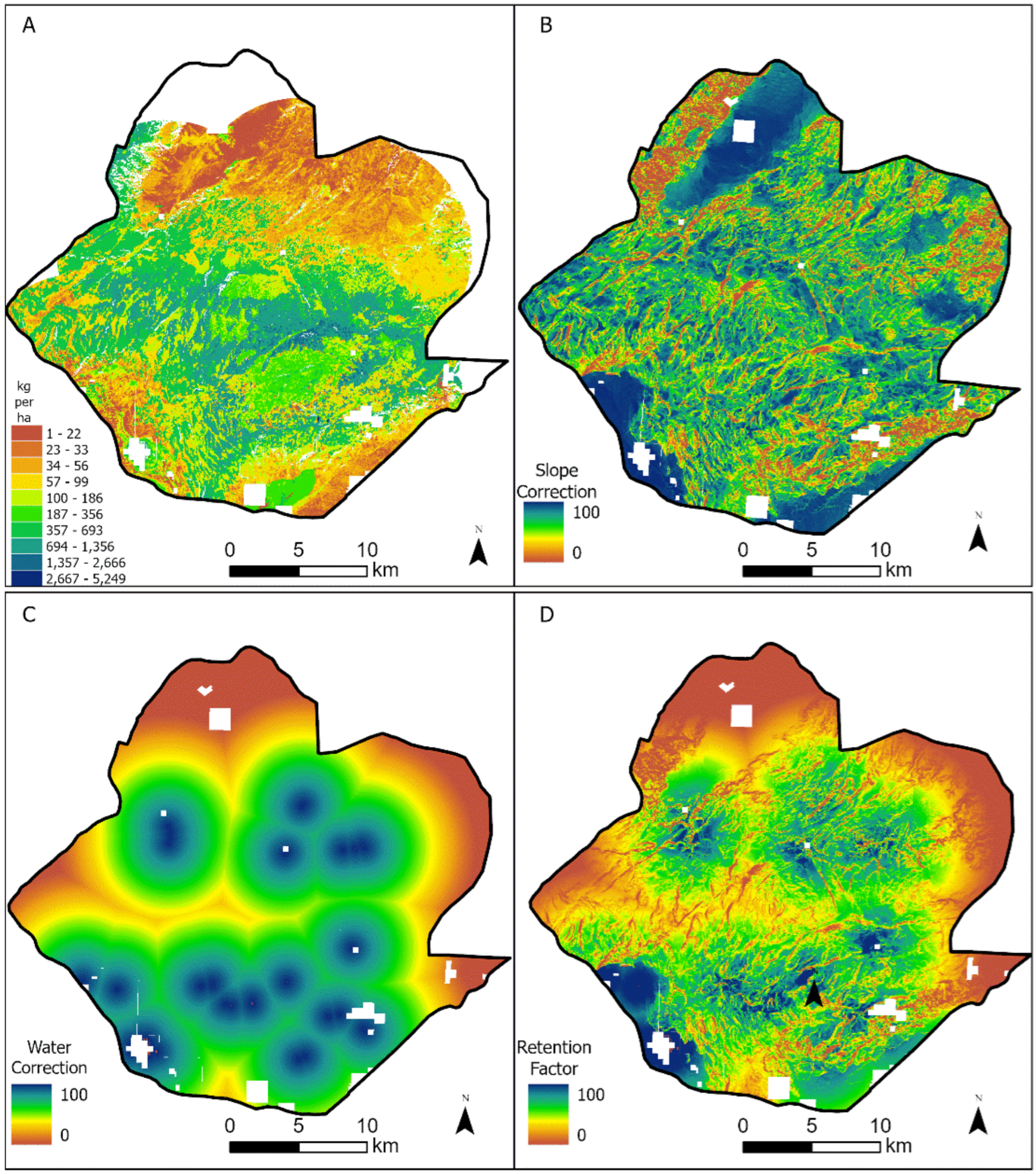
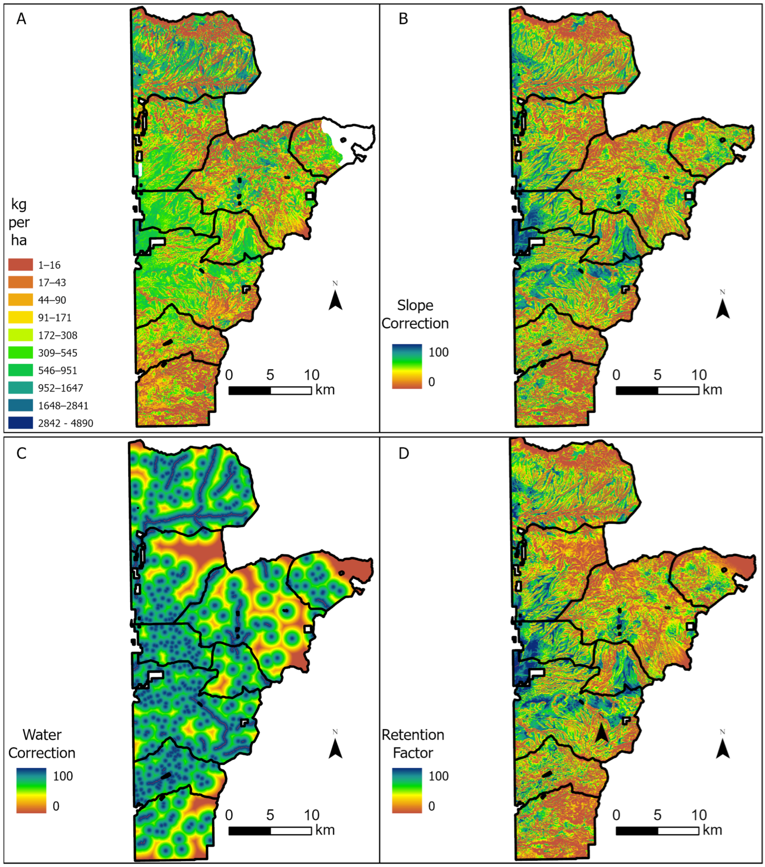
As a rule, estimating forage beneath forest canopies is not reliable with spectral remote sensing such as that used to derive the RPMS data. However, both study areas exhibit significant area occupied by trees (35% for MP and 19% for EC). Understory forage assessment is notably lacking across most of the western US [26,27] and relationships between overstory conditions and understory performance are highly variable and difficult to estimate reliably and consistently [28,29]. However, from previous unpublished efforts using field measurements, managers in the MP area estimated understory forage production as a function of overstory tree canopy as:

Understoryprod = m (x) + b

(6)

where Understoryprod is the estimated annual production in the understory, here in kg per ha; m is the slope of the line describing the rate of forage loss with increasing canopy cover; x is the estimated tree cover (provided by the RAP) in units of absolute foliar cover; and b is the y intercept. For the MP area, the slope and y intercept were −0.3695 and 20, respectively, while for EC the slope and intercept were −11.21 and 575. Note that the understory function is only invoked where no RPMS value exists (no data) or the tree cover is estimated to be above 25%. Reeves et al. [18] identified that remotely sensed estimates of annual production where tree canopy cover is ≥ 25% are not reliable. After consulting the management staff responsible for the EC area, it was determined that the above relationship was reasonable for this area as well. As a result, where tree cover was present, the amount of forage was estimated using this equation.

Next, the forage for annual forbs and grasses and perennial forbs and grasses are added to the adjusted amount for shrubs as follows:

Fractionalprodsum = (Fractionalprodshrubs + Fractionalprodafg + Fractionalprodpfg) or

Fractionalprodsum = (understoryprod)

where Fractionalprodsum is the total amount of forage estimated at a pixel, kg per ha; Fractionalprodshrubs is the annual production of shrubs adjusted for the estimated proportion of shrubs in the diet; Fractionalprodafg is the annual production by annual forbs and grasses; Fractionalprodpfg is the annual production by perennial forbs and grasses; and understoryprod is the estimated forage production under forested canopies. Estimates of tree production here are not used, since this component of production is deemed totally unpalatable and does not contribute to any part of the forage pool. Finally, the interaction of distance to water and slope constraints upon forage is represented as:

Totfor = Forret × Fractionalprodsum

(7)

where Totfor represents the total amount of forage available at a pixel accounting for terrain use constraints due to distance from water and slope steepness (here in kg per ha). When the total forage available at a given pixel (Totfor) has been estimated in units of kg per ha, the absolute amount of forage is given as:

Fractionalprodabs = Totfor/11.11

(8)

where Fractionalprodabs is the absolute amount of forage (in kg per ha) estimated at each pixel and the constant 11.11 is the number of pixels per ha in this analysis, since the pixel size is 30 m on each side. The value of Fractionalprodabs is then summed across each management unit, in this case grazing allotments, to yield a total estimate of available forage that has been corrected for terrain and water constraints, as well as shrub use and tree canopy cover assumptions.

The final component of the model involves accounting for the maximum amount of assumed use that can occur in a grazing allotment, and accounting for other management constraints such as the need to preserve forage for other wild or domestic ungulates inhabiting the area. Table 2 indicates that forage must be set aside in the MP case study to account for 1182 AUMs for cattle (tantamount to 418,194 kg of forage required), where their use of the landscape overlaps that of horses (Equus spp.). However, this was not an issue at EC, where only the domestic cattle were being evaluated. Furthermore, Table 2 indicates that in both study areas, the maximum allowable use was 30%, which is a common estimate for this parameter for federal land managers to use in most grazing allotments across the western US. Thus, for the MP area, the total amount of all forage in an allotment is constrained by the maximum allowable use of 30 percent and by the reserve requirement of 418,194 kg of forage, while the EC forage summation was constrained only by the allowable use estimate of 30 percent, since the use by wild ungulates was assumed to be negligible. The values for allowable use are derived at the discretion of the manager responsible for an allotment and are often developed in concert with multiple stakeholders.

The capacity estimate is obtained by dividing the total available forage supply by the unit of forage demand for a month defined as an animal unit month (AUM) of 354 kg per month (4246 kg per year) for EC. For Montgomery Pass, the monthly forage demand was given as 1.2 × AUM, because horses are slightly larger and have a higher forage amount requirement tantamount to 425 kg per month or 5095 kg per year (Table 1) [10]. In both study areas, animals are allowed to freely roam on an annual basis (e.g., yearlong grazing with no rest or rotation grazing management employed), so the estimated forage demand described in the results are based on a yearlong grazing plan.

3. Results

3.1. Eagle Creek

Although the AUM is the standard benchmark, when ungulates are wild or allowed to use the range for 12 months of the year, it is more useful to describe the number of animal units that are sustainable over the year. For the Eagle Creek study area, the estimated capacity (i.e., animal unit years; AUYs) for the average, above-average, and below-average forage scenarios was estimated as 1560, 2562, and 3575 animal units, respectively (18,715, 30,743, and 42,902 AUMs, respectively;

Table 3. Forage amounts for each study area and equivalent animal unit years.

	Eagle Creek			Montgomery Pass
	Low	Med	High	Low	Med	High
Average produciton (kg per ha) (Uncorrected from the RPMS)	245	416	587	147	226	304
Average produciton (kg per ha) (Corrected with retention factor)	95	162	229	54	83	112
Accounting for other herbivore needs (AUMS)	0	0	0	1182	1182	1182
Total Forage (kg) (includes RPMS production, shrub use assumptions and understory estimates)	37,211,406	61,126,400	85,300,883	6,660,361	10,275,821	14,285,117
Accounting for other herbivore needs (AUMS)	0	0	0	1182	1182	1182
	37,211,406	61,126,400	85,300,883	5,942,234	9,167,872	12,744,881
Capacity estimate (AUM)	18,715	30,743	42,902	6991	9826	13,659
Capacity estimate (AUY)	1560	2562	3575	175	287	398

). Here, this implies that the study area can support 1560 cattle on years when production is below average, 2652 on average, and 3575 on an above-average production year. Implicit in these estimates are the assumptions described above and listed in Table 1. The difference between the low and high production years was 239 percent, indicating that annual production across the study area exhibits very high interannual variability. The variability in average production ranged from 201 to 602 kg per ha, representing below-average and above-average production scenarios about a mean of 401 kg per ha. The spatial variability and connection between the landscape constraints of slope and distance to water can be seen in Figure 3. About 20 percent of the forage was considered unavailable (i.e., where the forage retention coefficient (Forret) equals 0), resulting from the interaction of distance from water and slope (Figure 3). Across the entire study area, the weighted average of the forage retention coefficient (Forret) was 0.35, meaning that, on average, the production values were multiplied by 0.35 percent. Likewise, Table 3 portrays the estimated forage response in average, below-average, and above-average scenarios, including the effects of the distance to water, slope and shrub use constraints. Unlike the Montgomery Pass study area, there is no correction or allocation of forage for other native herbivores assumed. These modeled stocking rate results compare favorably to the number of animals permitted to use the area on an annual basis.

3.2. Montgomery Pass

For the Montgomery Pass study area, the estimated capacity in AUYs for the average, above-average, and below-average forage scenarios was estimated as 176, 287, and 398 animal units, respectively (Table 3), which are tantamount to 6991, 9826, and 13,659 AUMs. Here, this implies that the study area can support 176 horses on years when production is below average, 287 on average, and 398 in an above-average production year. Implicit in these estimates are the assumptions described above and listed in Table 2. The difference between the low and high production years was 226 percent, indicating that annual production across the study area exhibits very high interannual variability, like EC. The temporal variability and connection between the landscape constraints of slope and distance to water can be seen in Panels B and D in Figure 4. About 11 percent of the forage was considered unavailable (i.e., where the forage retention coefficient equals 0), resulting from the interaction of distance from water and slope (Panel D, Figure 4). Across the entire study area, the weighted average of the forage retention coefficient was 0.41, meaning that, on average, the RPMS production values were multiplied by 0.41 percent when considering capacity (Panel C, Figure 4). Moreover, Table 3 portrays the estimated forage response in average, below-average, and above-average scenarios, including the effects of the distance to water, slope, and shrub use constraints. Unlike the Eagle Creek study area, there is no correction or allocation of forage for other native herbivores assumed.

4. Discussion

In conjunction with managers, data-driven decision support can guide sustainable grazing management and the promotion of animal welfare by supplying spatially and temporally continuous forage production information, overcoming many limitations of previous efforts to establish appropriate stocking rates and grazing capacity [10,17,18]. Here, we documented a decision support model to estimate grazing capacity, with demonstrated application in two case studies. With respect to MP, because the upper limit estimated in the capacity assessment was 398 horses and the current population is estimated at 654, it could be concluded that the area is over the Appropriate Management Level. For EC, the lower end of capacity was estimated at 1560 AUYs, or 1560 cattle for 12 months. This compares favorably with both the permitted and authorized number of cattle allowed to use forage resources in the study area. Overall, 2106 animal units are permitted in the area and between 2003 and 2021, while an average of 1090 AUYs were authorized to use the area. This figure is about 30% below the lower end estimate of capacity (Table 3), suggesting a conservative stocking rate is being used. Authorized use is almost always less than or equal to the permitted amount, as the permit dictates the upper end of animal use that can occur in an allotment. The authorized amount of herbivory varies substantially on an interannual basis in response to differing forage amounts, which is why it is so important to have tools that evaluate a range of forage conditions. It must be recognized that grazing capacity is highly dependent on many factors that vary seasonally, annually, or even over decades. Thus, estimates of grazing capacity are general approximations that are tempered with other information, experience, and judgment [2]. Grazing capacity estimates incorporate the kind and amount of vegetation (i.e., productivity), topography, infrastructure, multiple-use goals, and societal values.

While the underlying premise of this type of modeling approach is not new, new data sources such as those from the RAP and RPMS provide an unprecedented amount of information about the trends and disposition of vegetation for up to 40 years for coterminous US rangelands. Conventional grazing determinations rely heavily on production and utilization studies over multiple years. A minimum of three to five years of monitoring data is preferred, because forage production can vary substantially interannually [30]. However, the approach developed here evaluates forage response over decades rather than years, therefore providing a more reliable estimate of forage production and large herbivore capacity through a variety of temperature and precipitation regimes. Because these factors are addressed in a spatially explicit manner, they allow managers to evaluate forage production across a much larger area.

By applying this modeling approach, the process of AML determination is less time consuming and more comprehensive than conventional methods. The modeling approach encompasses multiple scenarios, using different assumptions about production patterns, water placement, forage preferences by different breeds of livestock, and forage reserve requirements for other species. The two study areas considered here differed in the assumptions used in the process and in terms of actual production observed in the RPMS dataset. The Eagle Creek study production values were substantially greater, even after the inclusion of modeled understory forage and use of shrubs in the diet, even though the forage retention value for EC was 15% less than that of the Montgomery Pass study area. This can be explained by the large assumption regarding the distance from water used in the MP, since horses were modeled as opposed to cattle; cattle have a lower tolerance for traveling long distances to water. In addition, the MP modeling invoked the understory assumption to estimate forage under a tree canopy (EQ. 6) on 35% of the landscape compared with 18% of the landscape in the EC study area. This is significant because the understory assumption for the MP resulted in small forage estimates in comparison to EC.

Our results and those of [13] suggest that patterns of herbivory and use on the landscape cannot be applied universally across breeds, terrain, or water access. Millward et al. [13] compared results from the process outlined by [10] and a newer method, employing Global Positioning System (GPS) to identify patterns of livestock use on the landscape, and found that, on average, the [10] approach resulted in a 14% lower stocking rate. Moreover, Holechek [10] intended these as general guidelines for setting initial stocking rates that could be later modified with experience in adaptive management style. With the advent and affordability of GPS tracking collars, the actual distribution of livestock on the landscape can be measured accurately and consistently, which can help managers improve their estimate of grazeable pasture area to determine annual stocking rate and could offer an improvement over the model developed here and the attendant assumed constraints to animal movement.

This modeling process acts distinctly as a decision support tool, because it enables different assumptions to be used to accommodate multiple viewpoints during the planning process. For example, if wild ungulate populations expand and require greater amounts of forage set aside, the model can easily accommodate that. Likewise, if different breeds of livestock (e.g., Bos indicus versus Bos taurus) may utilize shrubs quite differently and show different tolerances for distances to water, then these concerns can be easily evaluated in the model. Accordingly, our model, which also considers factors such as slope, canopy cover, and distance to water, enables a wide range of expected behaviors and tolerances by domestic and wild ungulates to be simulated.

In addition to being spatially explicit and addressing a wide range of temporal domains, the model presented here provides a repeatable and cost-effective process for establishing and adjusting capacity estimates and associated grazing plans that are supported by scientific information, with transparency for the public and stakeholders. This is important because the US Forest Service is required to consider management objectives and stakeholder input beyond those established for livestock grazing for a particular landscape when estimating grazing capacity. This approach can consider numerous other considerations, such as accommodating the presence of native ungulates or creating spatially explicit barriers to herbivory whether through natural (i.e., landform barriers) or administrative (i.e., areas of non-use) constraints. Critically, drought conditions may reduce forage and grazing capacity, and the model can assist with decision-making such as testing the tradeoffs between hauling water to areas with more forage versus feeding hay. The model process developed here is open and transparent and can be used for consensus building around key resource issues, such as deciding how many wild horses should be allowed to persist within the confines of management areas. Public land managers can test their assumptions about the reasonable numbers of animals permitted to use the landscape and whether relatively old management plans are still viable. Furthermore, by providing a range of suggested animal unit years based upon below, average, or above-average forage production, rangeland managers will be able to quickly adjust livestock numbers based upon predicted growing conditions or during drought mitigation response. Similarly, the capacity modeling approach can identify areas where water developments may increase grazing capacity, thereby optimizing limited funding for infrastructure such as water or cross fencing. This decision support system enables grazing plans to be modified in anticipation of changes in annual productivity over short-term or longer time horizons. Similarly, this kind of model can also be used for relatively new applications such as improving the valuation techniques of private grazing lands.

More specifically for U.S. federal lands, estimating capacity is a critical element of grazing permit administration as well as Forest Plan Revisions, providing information to fulfill the National Environmental Policy Act (NEPA) requirements. The Inyo National Forest will be using this work as it moves through the NEPA process and completes the revision of its 1988 Montgomery Pass Wild Horse Territory Management Plan. The AML Establishment and Adjustment Process includes three tiers: Tier 1—determine whether the four essential habitat components (forage, water, cover, and space) are present in sufficient amounts to sustain healthy wild horse and burro populations and healthy rangelands over the long-term. Tier 2—determine the amount of sustainable forage available for wild horse and burro use. Tier 3—determine whether the projected wild horse and burro herd size is sufficient to maintain genetically diverse wild horse and burro populations (i.e., avoid inbreeding depression). The process presented here helps address tiers 1 and 2.

Limitations and Future Work

A central issue not addressed in our approach is the evaluation of riparian conditions. The degradation of riparian areas can be caused through overuse by livestock [31,32,33]. The management of wild horses and burros on federal lands is somewhat unique because, unlike permitted livestock, wild horses and burros are largely free roaming and, as a result, controls over the timing, amount, and impacts of use are not easily managed [34]. Increased horse populations have led to increases in competition with wildlife and permitted cattle [35], in addition to contributing to conflict between multi-use objectives [36], especially in riparian areas where most grazing animals are naturally drawn to [32]. In numerous cases horses have been shown to limit or exclude the use of water sources by native wildlife [34]. This is particularly an issue in the Montgomery Pass area, where the estimated number of horses is 1.6 times greater than the modeled upper limit of capacity presented here.

A major assumption that warrants further discussion is that although this model estimates understory production, in situations where the study area is heavily forested, results will be heavily influenced by the understory assumptions based on expert opinions gained in specific areas. Understory production estimates used here were based on a limited number of unpublished plot level observations. It follows that decisions made in accordance with this inaccurate knowledge will be influential and potentially incorrect. National-, or even regional-level sampling efforts to describe understory vegetation performance are infrequent and insufficient for the type of production estimates needed here. Moreover, the results of the modeling process are dependent upon the quality of inputs, especially the remotely sensed inputs from the RPMS and RAP processes.

Future research to inform and improve the quality of forest understory data would be very beneficial to this modeling framework. One source to provide such data could be from the Forest Inventory and Analysis (FIA) database. The FIA program is managed by the USFS and is primarily focused on monitoring forested lands, which includes understory protocols. However, the frequency of these data in space (plots occur on all lands at about 5 km intervals in forested landscapes) and time (often, plots are only visited once every 10 years) are not optimal for estimating forage amounts across different vegetation types [27]. Moreover, production data are not collected and foliar cover data in the understory recorded using ocular estimates. Thus, converting the estimates of cover into production would require species-level estimates and allometric equations linking cover and height to production. These allometric equations are generally not created for non-forest understory species.

Applications such as Grasscast [37,38] or Fuelcast [18] provide forecasts of expected rangeland productivity within the current growing season, while the Dynamic Global Vegetation Model (DGVM) MC2 [39,40] projects rangeland production using climate-change scenarios. While improved projections of productivity will serve to only increase the utility of the approach developed here, more comprehensive data regarding understory forage performance that are collected by managers and stakeholders on the ground will enable greater accuracy overall in both forested and non-forested landscapes. Moreover, this approach is useful in other regions or countries, provided the remotely sensed estimates of vegetation and other required inputs are available.

5. Conclusions

The aim of our study was to develop a decision support tool with characteristics of the approach adopted by the authors of [10] but with an improved interaction between the slope and water constraints and provisions for understory forage calculations, and we achieved this aim. In addition, we demonstrated how newly available remotely sensed data sources describing vegetation cover and production can be incorporated into this spatially explicit approach demonstrated in two case studies. The impact of this work can be seen at https://www.stock-smart.com/; accessed on 24 November 2024, which is an online calculator that has adopted our approach; the impact of this work is still being assessed. Overall, greatly increased data availability and computer processing power enable the calculation of stocking rate estimates over potentially very large areas, while simultaneously considering both spatial and temporal variations in forage production, which has not previously been available at these scales. At the Eagle Creek study area, our estimated capacity (in AUYs) suggests that current authorized stocking rates are conservative by about 30%, given the present terrain, water dispersion, and forage productivity, when compared with the lower end of estimates our model suggested. In contrast, at the Montgomery Pass study area, our model indicated that the upper limit of stocking was 40% lower than the current estimated population of 654. Our approach builds upon the work of [10], but comparisons to other works are quite limited since, to our knowledge, this is a novel approach not developed elsewhere. The speed and precision of evaluating stocking rates using multiple assumptions and scenarios may enhance the ability of land managers to reevaluate allotment management plans or Forest Plans to account for decadal scale vegetation and climatic changes that may be occurring in a given region. The next steps to further develop this modeling approach could logically include (a) improving estimates of forage cover and production under tree canopies, (b) incorporating an increasing understanding of animal distribution and movement gained through the use of GPS collars, and (c) evaluating a large number of grazing allotments or pastures through comparisons of the estimated AUMs with the actual numbers currently utilizing the land. Such a comparison will help determine if large discrepancies occur, such as those found at the MP study site. Such improvements will further enable this model to leverage the utility of remote sensing-based estimates of forage production and incorporate present and future climate regime forecasts to efficiently quantify capacity and explore contrasting scenarios and assumptions.

References

1. Society of Range Management (SRM). Glossary of Terms Used in Range Management; Glossary Update Task Group: Denver, CO, USA, 1998; 32p. [Google Scholar]
2. Society for Range Management (SRM) Assessment and Monitoring Committee. Does Size Matter? Animal Units and Animal Unit Months. Rangelands 2017, 39, 17–19.
3. Ren, Y.; Zhu, Y.; Baldan, D.; Fu, M.; Wang, B.; Li, J.; Chen, A. Optimizing livestock carrying capacity for wild ungulate-livestock coexistence in a Qinghai-Tibet Plateau grassland. Sci. Rep. 2021, 11, 3635. [Google Scholar] [CrossRef]
4. John, A.C.; Rich, A.O.; Neil, E.W.; Jeffrey, C.M.; Michael, A.S.; Tom, D.W.; Richard, F.M.; Michael, A.G.; Chad, S.B. Ecology and management of sage-grouse and sage-grouse habitat. J. Range Manag. 2004, 57, 2–19. [Google Scholar]
5. Doherty, K.E.; Naugle, D.E.; Tack, J.D.; Walker, B.L.; Graham, J.M.; Beck, J.L. Linking conservation actions to demography: Grass height explains variation in greater sage-grouse nest survival. Wild. Biol. 2014, 20, 320–325. [Google Scholar] [CrossRef]
6. Smith, J.T.; Tack, J.D.; Doherty, K.E.; Allred, B.W.; Maestas, J.D.; Berkeley, L.I.; Dettenmaier, S.J.; Messmer, T.A.; Naugle, D.E. Phenology largely explains taller grass at successful nests in greater sage-grouse. Ecol. Evol. 2018, 8, 356–364. [Google Scholar] [CrossRef]
7. Clark, P.E.; Porter, B.A.; Pellant, M.; Dyer, K.; Norton, T.P. Evaluating the Efficacy of Targeted Cattle Grazing for Fuel Break Creation and Maintenance. Rangel. Ecol. Manag. 2023, 89, 69–86. [Google Scholar] [CrossRef]
8. Hudson, T.D.; Reeves, M.C.; Hall, S.A.; Yorgey, G.G.; Neibergs, J.S. Big landscapes meet big data: Informing grazing management in a variable and changing world. Rangelands 2021, 43, 17–28. [Google Scholar] [CrossRef]
9. Smith, L.; Ruyle, G.; Meyer, W.; Dyess, J.; Maynard, J.; Barker, S.; Williams, S.; Bell, D.; Lane, C.; Cassady, S.; et al. Arizona Guide to Rangeland Monitoring and Assessment. In Arizona Grazing Lands Conservation Association; Rio Nuevo Press: Tucson, AZ, USA, 2012; Available online: https://rangelandsgateway.org/sites/default/files/2021-01/guide-to-rangeland-monitoring-assessment.pdf (accessed on 16 May 2023).
10. Holechek, J.L. An approach for setting the stocking rate. Rangelands 1988, 10, 10–14. [Google Scholar]
11. Ganskopp, D.; Vavra, M. Slope use by cattle, feral horses, deer and bighorn sheep. Northwest Sci. 1987, 61, 74–81. [Google Scholar]
12. Winder, J.; Walker, D.; Bailey, C. Effect of breed on botanical composition of cattle diets on Chihuahuan desert range. J. Range Manag. 1996, 49, 209–214. [Google Scholar] [CrossRef]
13. Millward, M.F.; Bailey, D.W.; Cibils, A.F.; Holechek, J.L. A GPS-based Evaluation of Factors Commonly Used to Adjust Cattle Stocking Rates on Both Extensive and Mountainous Rangelands. Rangelands 2020, 42, 63–71. [Google Scholar] [CrossRef]
14. Hennig, J.D.; Rigsby, W.; Stam, B.; Scasta, J.D. Distribution of Salers cows in contrasting rangeland pastures relative to established slope and water guidelines. Livest. Sci. 2022, 257, 104843. [Google Scholar] [CrossRef]
15. Costanza, J.K.; Koch, F.H.; Reeves, M.C. Future Exposure of Forest Ecosystems to Multi-Year Drought in the United States. Ecosphere 2023, 14, e4525. [Google Scholar] [CrossRef]
16. National Research Council (NRC). Using Science to Improve the BLM Wild Horse and Burro Program: A Way Forward; The National Academies Press: Washington, DC, USA, 2013. [Google Scholar] [CrossRef]
17. Allred, B.W.; Bestelmeyer, B.; Boyd, C.S.; Brown, C.; Davies, K.W.; Duniway, M.; Ellsworth, L.M.; Erickson, T.A.; Fuhlendorf, S.D.; Griffiths, T.V.; et al. Improving Landsat predictions of rangeland fractional cover with multitask learning and uncertainty. Methods Ecol. Evol. 2021, 12, 841–849. [Google Scholar] [CrossRef]
18. Reeves, M.C.; Hanberry, B.B.; Wilmer, H.; Kaplan, N.E.; Lauenroth, W.K. An Assessment of Production Trends on the Great Plains from 1984 to 2017. Rangel. Ecol. Manag. 2021, 78, 165–179. [Google Scholar] [CrossRef]
19. Lubow, B. Memorandum: Statistical Analysis for 2020 Surveys of Wild Horse Abundance in Carson City District Office HMAs, and in Montgomery Pass JMA, January 25, 2022; U.S. Department of the Interior: Washington, DC, USA, 2020.
20. Henderson, E.B.; Bell, D.M.; Gregory, M.J. Vegetation mapping to support greater sage-grouse habitat monitoring and management: Multi-or univariate approach? Ecosphere 2019, 10, e02838. [Google Scholar] [CrossRef]
21. Jones, M.O.; Robinson, N.P.; Naugle, D.E.; Maestas, J.D.; Reeves, M.C.; Lankston, R.W.; Allred, B.W. Annual and 16-Day Rangeland Production Estimates for the Western United States. Rangel. Ecol. Manag. 2021, 77, 112–117. [Google Scholar] [CrossRef]
22. Conservation Biology Institute (CBI). Protected Areas Database of the United States (PADUS, CBI Edition 2.1). Available online: http://consbio.org/products/projects/pad-us-cbi-edition (accessed on 16 May 2023).
23. Jacoby, P.W.; Ueckert, D.N.; Hartmann, S. Control of Creosotebush (Larrea Tridentata) with Pelleted Tebuthiuron. Weed Sci. 1982, 30, 307–310. [Google Scholar] [CrossRef]
24. Hansen, R.; Clark, R.; Lawhorn, W. Foods of wild horses, deer, and cattle in the Douglas Mountain area, Colorado. Rangel. Ecol. Manag./J. Range Manag. Arch. 1977, 30, 116–118. [Google Scholar] [CrossRef]
25. Mueggler, W.F. Cattle distribution on steep slopes. Rangel. Ecol. Manag./J. Range Manag. Arch. 1965, 18, 255–257. [Google Scholar] [CrossRef]
26. Reeves, M.C.; Mitchell, J.E. A Synoptic Review of U.S. Rangelands: A Technical Document Supporting the Forest Service 2010 RPA Assessment; Gen. Tech. Rep. RMRS-GTR-288; U.S. Department of Agriculture, Forest Service, Rocky Mountain Research Station: Fort Collins, CO, USA, 2012; 128p.
27. Krebs, M.A.; Reeves, M.C.; Baggett, L.S. Predicting understory vegetation structure in selected western forests of the United States using FIA inventory data. For. Ecol. Manag. 2019, 448, 509–527. [Google Scholar] [CrossRef]
28. LaRade, S.; Bork, E. Aspen forest overstory relations to understory production. Can. J. Plant Sci. 2011, 91, 847–851. [Google Scholar] [CrossRef]
29. Balandier, P.; Mårell, A.; Prévosto, B.; Vincenot, L. Forest understorey and overstorey interactions: So much more than just light interception by trees. For. Ecol. Manag. 2022, 526, 120584. [Google Scholar] [CrossRef]
30. United States Department of the Interior (DOI); Bureau of Land Management (BLM). Wild Horses and Burros Management Handbook; BLM Handbook H-4700-1; Bureau of Land Management (BLM): Washington, DC, USA, 2010; 80p.
31. Bailey, D.W.; Trotter, M.G.; Tobin, C.; Thomas, M.G. Opportunities to Apply Precision Livestock Management on Rangelands. Front. Sustain. Food Syst. 2021, 5, 515–523. [Google Scholar] [CrossRef]
32. Burdick, J.; Swanson, S.; Tsocanos, S.; McCue, S. Lentic Meadows and Riparian Functions Impaired After Horse and Cattle Grazing. J. Wild. Manag. 2021, 85, 1121–1131. [Google Scholar] [CrossRef]
33. Cubley, E.S.; Richer, E.E.; Baker, D.W.; Lamson, C.G.; Hardee, T.L.; Bledsoe, B.P.; Kulchawik, P.L. Restoration of riparian vegetation on a mountain river degraded by historical mining and grazing. River Res. Appl. 2022, 38, 80–93. [Google Scholar] [CrossRef]
34. Davies, K.W.; Boyd, C.S. Ecological Effects of Free-Roaming Horses in North American Rangelands. BioScience 2019, 69, 558–565. [Google Scholar] [CrossRef]
35. Scasta, J.D.; Hennig, J.D.; Beck, J.L. Framing Contemporary U.S. Wild Horse and Burro Management Processes in a Dynamic Ecological, Sociological, and Political Environment. Hum.–Wildl. Interact. 2018, 12, 6. [Google Scholar] [CrossRef]
36. Beever, E.; Aldridge, C. Influences of Free-Roaming Equids on Sagebrush Ecosystems, with a Focus on Greater Sage-Grouse. Stud. Avian Biol. 2011, 38, 273–290. [Google Scholar]
37. Hartman, M.D.; Parton, W.J.; Derner, J.D.; Schulte, D.K.; Smith, W.K.; Peck, D.E.; Day, K.A.; Del Grosso, S.J.; Lutz, S.; Fuchs, B.A.; et al. Seasonal grassland productivity forecast for the U.S. Great Plains using Grass-Cast. Ecosphere 2020, 11, e03280. [Google Scholar]
38. Peck, D.; Derner, J.; Parton, W.; Hartman, M.; Fuchs, B. Flexible stocking with Grass-Cast: A new grassland productivity forecast to translate climate outlooks for ranchers. West. Econ. Forum 2019, 17, 24–39. [Google Scholar] [CrossRef]
39. Bachelet, D.; Ferschweiler, K.; Sheehan, T.J.; Sleeter, B.M.; Zhu, Z. Projected carbon stocks in the conterminous USA with land use and variable fire regimes. Glob. Change Biol. 2015, 21, 4548–4560. [Google Scholar] [CrossRef]
40. Kim, J.B.; Kerns, B.K.; Drapek, R.J.; Pitts, G.S.; Halofsky, J.E. Simulating vegetation response to climate change in the Blue Mountains with MC2 dynamic global vegetation model. Clim. Serv. 2018, 10, 20–32. [Google Scholar] [CrossRef]
Figure 1. The study areas associated with the two case studies including the Montgomery Pass Wild Horse and Burro Territory (Panel A), and the grazing allotments associated with the Eagle Creek Ranger District, Apache−Sitgreaves National Forest (Panel B). The legend applies to both panels.
Land 14 00140 g001
Figure 2. Main inputs, model assumptions, and flow of data through the capacity model.
Land 14 00140 g002
Figure 3. The results from the MP modeling process. Panel (A) depicts the annual production after the combined effects of slope, water, and shrub use have been accounted for. Panel (B) depicts the effect of slope as a reduction to forage availability. Panel (C) depicts the effect of water availability as a reduction to forage availability. Panel (D) depicts the combined (multiplicative) effect of slope as a reduction to forage availability. White is either private land or has a retention factor of 0 (no forage is available).
Land 14 00140 g003
Figure 4. The results from the EC modeling process. Panel (A) depicts the annual production after the combined effects of slope, water, and shrub use have been accounted for. Panel (B) depicts the effect of slope as a reduction to forage availability. Panel (C) depicts the effect of water availability as a reduction to forage availability. Panel (D) depicts the combined (multiplicative) effect of slope as a reduction to forage availability. White is either private land or has a retention factor of 0 (no forage is available).
Land 14 00140 g004